Identification of Thresholds on Population Density for Understanding Transmission of COVID‐19

Abstract

Pathways of transmission of coronavirus (COVID‐19) disease in the human population are still emerging. However, empirical observations suggest that dense human settlements are the most adversely impacted, corroborating a broad consensus that human‐to‐human transmission is a key mechanism for the rapid spread of this disease. Here, using logistic regression techniques, estimates of threshold levels of population density were computed corresponding to the incidence (case counts) in the human population. Regions with population densities greater than 3,000 person per square mile in the United States have about 95% likelihood to report 43,380 number of average cumulative cases of COVID‐19. Since case numbers of COVID‐19 dynamically changed each day until 30 November 2020, ca. 4% of US counties were at 50% or higher probability to 38,232 number of COVID‐19 cases. While threshold on population density is not the sole indicator for predictability of coronavirus in human population, yet it is one of the key variables on understanding and rethinking human settlement in urban landscapes.

Key Points

• Based on data from the USA, the population density of 1,192 persons per square mile represented a 50% or higher probability of more than 38,000 COVID‐19 cumulative cases at county scale as of 30 November 2020

• About 35 counties in the USA with population density greater or equal to 3,000 per square mile are at very high chances (95% or higher) of more than 43,000 cumulative cases at county scale as of 30 November 2020

• Analysis shows the vulnerability of urban towns to respiratory infectious disease

1. Introduction

Severe Acute Respiratory Syndrome caused by Coronavirus (SARS‐CoV‐2 thereafter) is a respiratory lung infection, and as of 28 April 2021, there have been more than 148 million (WHO COVID‐19 Dashboard, 2021, https://covid19.who.int/) confirmed human cases in the world. The SARS‐CoV‐2 virus remains highly infectious and is circulating in the human population at an alarming rate with anticipated variants in near future. An emerging disciplinary consensus is that seasonal variation may lead to cyclical outbreaks in the human population (Carlson et al., 2020; Merow & Urban, 2020). As with all airborne respiratory infectious diseases, the transmission of SARS‐CoV‐2 is high in densely populated urban regions of the world (Cruickshank, 1939; Robinson et al., 2012). However, thresholds of population density relative to the outbreak of the disease in humans remains unknown. The relative importance of knowledge of threshold on population density with reference to infectious disease such as COVID‐19 is important for the future of modern cities and urban landscapes in the USA, given about 71% of the population reside in urbanized areas with an average density of 2,534 persons per square mile (https://www.census.gov/programs-surveys/geography/guidance/geo-areas/urban-rural/ua-facts.html).

Influenza transmission dynamics, which allow parallel comparison with COVID‐19 transmission, depend on several socio‐demographic factors (such as race, income level, education, and location), but population density remains a critical variable for controlling an outbreak of seasonal influenza (Atkinson & Wein, 2008; Merler & Ajelli, 2010). While the severity of airborne contagion cannot be attributed solely to population density (Li et al., 2018), the knowledge of thresholds on population density can be helpful in understanding the spatial distribution with respect to the risk of disease (Chandra et al., 2013; Grantz et al., 2016). Intuitively, high population density is concluded to favor contagion and vice‐versa. However, non‐uniform distribution of a population can yield inconclusive results (Li et al., 2018). While the significant association was reported between population density and transmissibility for the 1,918 influenza pandemic in Chicago (Grantz et al., 2016), the average influenza attack rates decreased with increasing population density in Japan (Hoyle & Wickramasinghe, 1990). In the context of COVID‐19, an analysis of Brazilian data suggests the general increase in COVID‐19 cases was associated with highly populated regions (Pequeno et al., 2020). There is no study to date that provides an exploratory association of population density thresholds with COVID‐19 cases in the continental USA.

This study was undertaken to determine thresholds on population density that can be used to estimate the probable case load from COVID‐19. Estimation of a threshold population density would allow in the differentiation of probabilistic low and high‐case regions and offer useful input for planning, designing, and targeting public health interventions. Also, identifying specific regions where greater surveillance is required to contain the disease would be enhanced and can be used to define the expansion of urbanized areas in the USA.

2. Methods

Daily incidence data for COVID‐19 cases in the 3,107 mainland U.S. counties were obtained from the GitHub project (“The New York Times. (2021). Coronavirus (Covid‐19) Data in the United States,” 2021) (https://github.com/nytimes/covid-19-data) from 15 March 2020, to 30 November 2020. The time period was selected based on the non‐availability of vaccines since vaccines will mask the limit on population densities. Data on the population densities of each U.S. county were obtained from the U.S. Census Bureau (2019) (https://www.census.gov/data/datasets/time-series/demo/popest/2010s-counties-total.html). Land area in square miles was obtained from the U.S. Census Bureau (https://www.census.gov/library/publications/2011/compendia/usa-counties-2011.html#LND). An ordinal logistic regression model was employed to study the dependency of COVID‐19 cases (thereafter cases) on counties' population density. It was assumed that the population densities remained constant during the study period, implying population mobility has minimal impact on population density. Further, the population was assumed to be uniformly distributed over the county. Since the number of cases differs widely over the county, intuitively, it is preferable to classify cases into a number of classes where each class explicitly implies a specific range of case load. To classify cases, we estimated the percentile of cumulative cases at an interval of 15 days beginning 15 March 2020, to 30 November 2020. Cumulative cases data were divided into three categories (or events): (a) low number of cases (up to 80th percentile); (b) medium number of cases (80th to 95th percentile); and (c) high number of cases (greater than 95th percentile). The 80th percentile case on 30 November 2020 was 3,817 (Table 1), which can still be considered relatively less compared to the number of cases in high‐risk locations.

Table 1.

Biweekly 80th Percentile Cases of Low Cases

Date	80th percentile cases
15 March 2020	0
31 March 2020	15
15 April 2020	63
30 April 2020	126
15 May 2020	196
31 May 2020	271
15 June 2020	351
30 June 2020	480
15 July 2020	670
31 July 2020	970
15 August 2020	1,175
31 August 2020	1,382
14 September 2020	1,564
30 September 2020	1,787
15 October 2020	2,069
31 October 2020	2,410
15 November 2020	3,036
30 November 2020	3,817

Moreover, a higher value for the log‐likelihood (a statistical metric used for model selection) in Table 2, justifies the choice of the 80th percentile. In fact, the log‐likelihood function was found to be better with increasing percentile, with the increase being less for the percentiles above the value of 80.

Table 2.

Variation in Log‐Likelihood in COVID‐19 Cases

Percentile up to which cases were considered low	Log likelihood
33	−3,070.07
50	−2,860.07
80	−1,634.02
85	−1,364.49

Thus, the ‘‘reasonable’’ choice of percentiles for classification of cases will lead to overall similar model results without altering the final interpretation. The following paragraph briefly explains the analysis approach. Relevant theory for the application of ordinal logistic regression is detailed in the supplementary section.

The predictor used is the county population density which is the county's population per unit of the county's land area. The response variable, which is ordinal in nature, is the cumulative case count classified into low, medium, and high (based on percentiles). Logit link function (details in supplementary section) was used to express the dependent variable as a linear function of the independent variables. Link function also relates the response (ordinal cases) to linear predictor (population density) and transforms the probabilities of ordinal response to the continuous scale (0,1). The regression equations, thus, take the form as follows:

$$\ln \left(\frac{p\left(\mathrm{h}\mathrm{i}\mathrm{g}\mathrm{h}\mathrm{c}\mathrm{a}\mathrm{s}\mathrm{e}\mathrm{s}\right)}{1-p\left(\mathrm{h}\mathrm{i}\mathrm{g}\mathrm{h}\mathrm{c}\mathrm{a}\mathrm{s}\mathrm{e}\mathrm{s}\right)}\right)={\alpha }_1+\beta \ast \mathrm{p}\mathrm{o}\mathrm{p}\mathrm{u}\mathrm{l}\mathrm{a}\mathrm{t}\mathrm{i}\mathrm{o}\mathrm{n}\mathrm{d}\mathrm{e}\mathrm{n}\mathrm{s}\mathrm{i}\mathrm{t}\mathrm{y}$$ (1)

$$\ln \left(\frac{p\left(\mathrm{m}\mathrm{e}\mathrm{d}\mathrm{i}\mathrm{u}\mathrm{m}\mathrm{c}\mathrm{a}\mathrm{s}\mathrm{e}\mathrm{s}\right)}{1-p\left(\mathrm{m}\mathrm{e}\mathrm{d}\mathrm{i}\mathrm{u}\mathrm{m}\mathrm{c}\mathrm{a}\mathrm{s}\mathrm{e}\mathrm{s}\right)}\right)={\alpha }_2+\beta \ast \mathrm{p}\mathrm{o}\mathrm{p}\mathrm{u}\mathrm{l}\mathrm{a}\mathrm{t}\mathrm{i}\mathrm{o}\mathrm{n}\mathrm{d}\mathrm{e}\mathrm{n}\mathrm{s}\mathrm{i}\mathrm{t}\mathrm{y}$$ (2)

where p(high cases) and p(medium cases) are the probabilities of high and medium cases, respectively. Constants and coefficients in Equations (1, 2) were estimated using the maximum likelihood estimation methods. Since the total probabilities sum up to one, the probability of a low number of cases were estimated by subtracting the probability of high and medium cases.

3. Results and Discussion

We start our analysis with results obtained from logistical regression models (Figure 1) showing three critical statistical metrics (Somers D, Goodman‐Kruskal Gamma and Percent Concordant pairs).

Figure 1.

Performance of logistical regression model on a biweekly scale for the entire USA.

High values of measures of association (>82%), that is, percentage of concordant pairs, Somers's D and Goodman‐Kruskal Gamma, signify that the performance of ordinal logistic model is satisfactory. On average, model performance remained constant since start of collection of data on COVID‐19 human cases. The p‐values for each constant and predictor population density were less than 0.05 (not shown), thus establishing statistical significance. The p‐value for the test of all slopes is zero (Table S1 in Supporting Information S1), which indicates the predictor population density has a statistically significant relationship with the response variable (COVID‐19 cases). The deviance goodness of fit result (p > 0.05), for all dates for which the model was run, showed adequate fit for the data, and the associated probabilities do not deviate significantly from observed values (detailed inference of model performance indicators for 15 November 2020 is presented in Table S1 in Supporting Information S1). The model results for any one day should sufficiently explain the behavior of event probability (cases) with population density. The plots in Figure 2 show average probability of high, medium, and low number of cases.

Figure 2.

Average probability versus population density for (a) High (b) Medium (c) Low number of cases, from 15 March 2020, to 30 November 2020.

Average probabilities were defined as the mean of the probabilities obtained from the ordinal logistic regression models for each of the eighteen bi‐weekly cases (from 15 March 2020, to 30 November 2020). The monotonic nature of Figure 2a shows that with an increasing population density, the probability of a high number of cases increases, and vice versa. The probability rises steeply to a nearly constant value of 1 at a population density of ca. 5,000 per square mile, suggesting population densities greater than this value were remarkably associated with the corresponding high number of COVID‐19 cases. The implication is that the pronounced effect of high population density and a proportional number of cases was sufficient to establish population density as an important factor in transmission potential of this disease. The results suggest that in densely populated areas, it may be challenging to follow social distancing norms, thus an increased number of COVID‐19 human cases were to be expected. Figure 2c shows the probability of a low number of cases, a trend opposite to that for high number of cases. The probability continuously decreases to a constant value close to zero, signifying that as population density increases, the chance of a low number of cases decreases. Figure 2b illustrates the medium number of cases with population density. The maximum probability of the medium number of cases is ca. 0.48, corresponding to the population density of ca. 1,190 per square mile. Thus, a decrease in population density from 1,190 per square mile decreases the probability of a medium number of cases as the probability of low number of cases increase. On the other hand, if population density increases beyond 1,190 per square mile, the probability for a medium number of cases decreases since probability of high number of cases increase thereafter. Population density of 1,190 people per square mile can be interpreted as a transition from low to high COVID‐19 cases. Figure 3 illustrates changes in event probabilities over time and suggests that even low‐density counties are likely to be more vulnerable as the probability of high number of COVID‐19 cases for population density increases over time.

Figure 3.

Changes in bi‐weekly probability from 15 March 2020, to 30 November 2020 of (a) high, (b) medium, and (c) low number of COVID‐19 cases.

In Figure 2a, the threshold population density is shown at which a 50% chance of a high number of cases will occur, ca. 1,622 per square mile. The population density for getting a low number of cases at 50% chance is 762 per square mile (Figure 2c), and the arithmetic mean of these two values at high and low cases gives an average of 1,192 per square mile and defined as the population density at which there is a 50% chance of average number of cases. The average number of cases is estimated by averaging cumulative cases in counties with population density greater than the threshold of 1,192 per square mile. Thus, 4.02% (125 of 3,107) of the counties with population density greater than 1,192 per square mile are at 50% or greater risk of 38,232 COVID‐19 cases as on 30 November 2020. The key results discussed here are concisely summarized in Table 3.

Table 3.

Key Results of Population Density‐Cases Analysis

Attribute	Value
Population density beyond which 95% probability of high number of cases	3,000 per square mile
Population density beyond which 50% probability of high number of cases	1,622 per square mile
Average Population density beyond which 50% probability of average number of cases	1,192 per square mile
Percentage of US counties at greater than 50% probability of average number of cases	4.02% (125 out of 3,107)

Table 4 provides values for population density and arithmetic average probability of high number of cases for each state in the US, as of 30 November 2020.

Table 4.

Probabilities of High Number of COVID19 Cases as of 30 November 2020

State	Population density (per square mile)	Average probability of high cases (Ap)	Maximum probability of high cases (map)	Minimum probability of high cases (minp)	Rank of Ap	Rank of map	Percent difference between map and Ap
District of Columbia	11,569.7	1	1	1.000	1	1	0
New Jersey	1,207.8	0.404	1	0.027	2	1	60
Rhode Island	1,024.5	0.28	0.652	0.043	3	23	57
Massachusetts	883.5	0.242	1	0.022	4	1	76
Connecticut	736.6	0.156	0.421	0.028	7	27	63
Maryland	622.9	0.165	1	0.019	6	1	84
Delaware	499.6	0.144	0.368	0.030	8	29	61
New York	412.8	0.099	1	0.017	11	1	90
Florida	400.7	0.078	0.981	0.018	13	14	92
Pennsylvania	286.1	0.079	1	0.018	12	1	92
Ohio	286.1	0.066	0.927	0.019	14	18	93
California	253.7	0.12	1	0.017	10	1	88
Illinois	228.2	0.047	0.999	0.018	18	10	95
Hawaii	220.3	0.121	0.52	0.018	9	26	77
Virginia	216.1	0.232	1	0.018	5	1	77
North Carolina	215.7	0.041	0.711	0.018	20	20	94
Indiana	187.9	0.038	0.857	0.018	24	19	96
Georgia	184.6	0.051	0.93	0.018	15	17	95
Michigan	176.7	0.048	0.944	0.018	17	16	95
South Carolina	171.2	0.027	0.077	0.018	32	35	65
Tennessee	165.6	0.031	0.346	0.018	28	30	91
New Hampshire	151.9	0.029	0.053	0.018	31	39	45
Washington	114.6	0.03	0.181	0.017	30	33	83
Kentucky	113.1	0.031	0.706	0.018	28	21	96
Texas	111	0.036	0.952	0.017	27	15	96
Louisiana	107.6	0.04	0.689	0.018	22	22	94
Wisconsin	107.5	0.038	0.993	0.018	24	12	96
Alabama	96.8	0.022	0.071	0.018	37	36	69
Missouri	89.3	0.037	0.999	0.018	26	10	96
West Virginia	74.6	0.023	0.046	0.018	35	42	50
Minnesota	70.8	0.043	0.984	0.017	19	13	96
Vermont	67.7	0.021	0.036	0.018	39	46	42
Arizona	64.1	0.021	0.053	0.018	39	39	60
Mississippi	63.4	0.02	0.042	0.017	42	44	52
Arkansas	58	0.02	0.059	0.018	42	38	66
Oklahoma	57.7	0.025	0.225	0.017	33	32	89
Iowa	56.5	0.021	0.118	0.018	39	34	82
Colorado	55.6	0.049	1	0.017	16	1	95
Oregon	43.9	0.039	0.637	0.017	23	24	94
Maine	43.6	0.022	0.038	0.018	37	45	42
Utah	39	0.041	0.414	0.017	20	28	90
Kansas	35.6	0.023	0.272	0.017	35	31	92
Nevada	28.1	0.02	0.043	0.017	42	43	53
Nebraska	25.2	0.025	0.527	0.017	33	25	95
Idaho	21.6	0.019	0.048	0.017	46	41	60
New Mexico	17.3	0.02	0.069	0.017	42	37	71
South Dakota	11.7	0.018	0.03	0.017	47	47	40
North Dakota	11	0.018	0.022	0.017	47	48	18
Montana	7.3	0.018	0.02	0.017	47	49	10
Wyoming	6	0.018	0.019	0.017	47	50	5

This average probability is the simple arithmetic average of the respective probabilities of state counties. It is intuitive that the most densely populated states were also those with the highest probability of a high number of cases, strengthening the finding that population density is critical beyond a specific threshold. The average probability for a high number of COVID‐19 cases provides a number useful for conceptualizing the overall risk of infection in a particular state. However, except for a few densely populated states, epicenter counties are not highlighted. For example, on 30 November 2020, Texas, California, Florida, and Illinois were States with the largest number of COVID‐19 cases. From Table 4, it was obvious that the relatively low values of average probabilities for those four states do not reflect their epicenter status. Therefore, we defined the maximum average probability for a state which is taken equal to the maximum value of average probabilities considering all the counties of a state. Thus, the maximum average probability for each state as calculated. The high probability of a high number of cases (>90%) indicated this metric performed acceptably to rank a state as an epicenter. Exceptions were noted, where relatively low value of maximum average probability of high cases was observed in low population density states having high number of COVID‐19 cases. This anomaly is a potential limitation of the logistical regression methods, in dealing with locations with low population densities and high cases. However, it is understood that any regressive model considering population density as the single explanatory variable likely would fail to explain a high number of cases in less densely populated regions. Lastly, an important observation with reference to population density and case analysis can be discerned from Table 4, namely the percentage difference between the maximum and average probabilities of high number of cases, being very high for many states, notably those with high maximum average probabilities. This signifies that only a few counties of the state account for a large number of cases, and the state as a whole would not be an epicenter of COVID‐19.

The analysis in our study assumes a uniform population distribution. In reality, the population is generally not distributed evenly across the county, as most of the population clusters in and around cities. The lack of a standard sub‐county level case count, which rules out the possibility of conducting a more realistic city‐level threshold analysis, forms a limitation of our study. Furthermore, though county population density is generally considered a reliable predictor to explain COVID‐19 cases due to its high explanatory power (Riley, 2007; Wong & Li, 2020), controlling it for other variables such as population size could bring valuable insights to determine running thresholds on population density.

4. Conclusions and Implications on Future of Urban Cities

The interrelationship of population density with the number of COVID‐19 cases was analyzed, with the objective to determine thresholds for population density above which there was a 50% or greater chances of observing greater than average number of COVID‐19 cases in humans. Population density and COVID‐19 cases, when analyzed together, suggest ca. 4% of the counties (shown in Figure 4) in the United States would be at 50% or greater chances of observing greater than average number of COVID‐19 cases and confined to a few counties.

Figure 4.

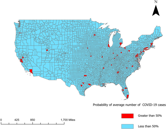
US counties with greater than 50% probability of average number of cases as of 30 November 2020.

The thresholds provide useful information as a guide for city planners. The current urbanization system is such that many big cities form clusters (Angel & Blei, 2016), and location‐wise, most of these clusters happen to coincide with the counties having population density greater than the threshold. For example, New York City and San Francisco where nationwide highest COVID‐19 cases were reported, are the densest counties of the nation. This apparent agglomeration of cities may be contributing to rapid spread of the disease since it is difficult to avoid interaction between infected and susceptible populations. The disproportionate distribution of disease burden can therefore be linked to the existing non‐uniform concentration of urban landscapes.

This link suggests that current building stocks are vulnerable to infectious diseases and is suggestive of innovation in redesigning of urban landscapes from the standpoint of a resilient public health infrastructure.

However, this observation is essentially a preliminary one at this stage to establish such a causal link. Therefore, it is recommended to undertake relevant town planning studies concerning population redistribution, which could bring about necessary changes to build community resilience for future epidemics/pandemics.

In combination with other governing factors, the population density threshold can provide a decisive conclusion, notably for estimating cases and mitigating COVID‐19 in human populace, especially for urban neighborhoods that are more likely heterogenous in race, income, and infrastructure (Maantay & Maroko, 2009; Maantay et al., 2007). Dense populations comprise sub‐populations, namely communities of color and low‐income communities that are vulnerable, for example, poor housing, high pollution, lack of access to health care, and a higher rate of pre‐existing conditions (Brulle & Pellow, 2006; Bullard, 2005; Pellow, 2000). Nevertheless, the relationship between population density and case loads is sufficiently robust that it can be employed by policymakers to prepare anticipatory plans for specific communities and thereby prevent the spread of infection and mitigate the effects of the disease.

Conflict of Interest

The authors declare no conflicts of interest relevant to this study.

Supporting information

Supporting Information S1

Jamal, Y. , Gangwar, M. , Usmani, M. , Adams, A. E. , Wu, C.‐Y. , Nguyen, T. H. , et al. (2022). Identification of thresholds on population density for understanding transmission of COVID‐19. GeoHealth, 6, e2021GH000449. 10.1029/2021GH000449

Data Availability Statement

Raw data sets are publicly available and can be accessed using weblinks provided. Datasets generated in this study are available on openly accessible data servers. https://github.com/nytimes/covid-19-data. https://www.census.gov/data/datasets/time-series/demo/popest/2010s-counties-total.html. https://www.census.gov/library/publications/2011/compendia/usa-counties-2011.html#LND. While there are many other links to get the data on COVID‐19 case numbers, to the best of our knowledge, GitHub is the only concise yet comprehensive source which provides easy to analyze chronological case count data for US at county scale. All the data analysis was performed using the MINITAB software package, a standard package for statistical analysis available at https://www.minitab.com/en-us/products/minitab/.

References

- Angel, S. , & Blei, A. M. (2016). The spatial structure of American cities: The great majority of workplaces are no longer in CBDs, employment sub‐centers, or live‐work communities. Cities, 51, 21–35. 10.1016/j.cities.2015.11.031 [DOI] [Google Scholar]
- Atkinson, M. , & Wein, L. (2008). Quantifying the routes of transmission for pandemic influenza. Bulletin of Mathematical Biology, 70(3), 820–867. 10.1007/s11538-007-9281-2 [DOI] [PubMed] [Google Scholar]
- Brulle, R. J. , & Pellow, D. N. (2006). Environmental justice: Human health and environmental inequalities. Annual Review of Public Health, 27(102), 103–124. 10.1146/annurev.publhealth.27.021405.102124 [DOI] [PubMed] [Google Scholar]
- Bullard, R. (2005). Environmental justice in the 21st century. Debating the Earth. [Google Scholar]
- Carlson, C. J. , Gomez, A. C. R. , Bansal, S. , & Ryan, S. J. (2020). Misconceptions about weather and seasonality must not misguide COVID‐19 response. Nature Communications, 11(1), 2–5. 10.1038/s41467-020-18150-z [DOI] [PMC free article] [PubMed] [Google Scholar]
- Chandra, S. , Kassens‐Noor, E. , Kuljanin, G. , & Vertalka, J. (2013). A geographic analysis of population density thresholds in the influenza pandemic of 1918‐19. International Journal of Health Geographics, 12, 1–10. 10.1186/1476-072X-12-9 [DOI] [PMC free article] [PubMed] [Google Scholar]
- Cruickshank, R. (1939). Air‐borne infection and its prevention. Public Health, 53(C), 254–255. 10.1016/S0033-3506(39)80180-9 [DOI] [Google Scholar]
- Grantz, K. H. , Rane, M. S. , Salje, H. , Glass, G. E. , Schachterle, S. E. , & Cummings, D. A. (2016). Disparities in influenza mortality and transmission related to sociodemographic factors within Chicago in the pandemic of 1918. Proceedings of the National Academy of Sciences, 113(48), 13839–13844. 10.5061/dryad.48nv3 [DOI] [PMC free article] [PubMed] [Google Scholar]
- Hoyle, F. , & Wickramasinghe, N. C. (1990). Influenza ‐ Evidence against contagion: Discussion paper. Journal of the Royal Society of Medicine, 83(4), 258–261. 10.1177/014107689008300417 [DOI] [PMC free article] [PubMed] [Google Scholar]
- Li, R. , Richmond, P. , & Roehner, B. M. (2018). Effect of population density on epidemics. Physica A: Statistical Mechanics and its Applications, 510, 713–724. 10.1016/j.physa.2018.07.025 [DOI] [Google Scholar]
- Maantay, J. , & Maroko, A. (2009). Mapping urban risk: Flood hazards, race, & environmental justice in New York. Applied Geography, 29(1), 111–124. 10.1016/j.apgeog.2008.08.002 [DOI] [PMC free article] [PubMed] [Google Scholar]
- Maantay, J. A. , Maroko, A. R. , & Herrmann, C. (2007). Mapping population distribution in the urban environment: The cadastral‐based expert dasymetric system (CEDS). Cartography and Geographic Information Science, 34(2), 77–102. 10.1559/152304007781002190 [DOI] [Google Scholar]
- Merler, S. , & Ajelli, M. (2010). The role of population heterogeneity and human mobility in the spread of pandemic influenza. Proceedings of the Royal Society B: Biological Sciences, 277(1681), 557–565. 10.1098/rspb.2009.1605 [DOI] [PMC free article] [PubMed] [Google Scholar]
- Merow, C. , & Urban, M. C. (2020). Seasonality and uncertainty in global COVID‐19 growth rates. Proceedings of the National Academy of Sciences of the United States of America, 117(44), 27456–27464. 10.1073/pnas.2008590117 [DOI] [PMC free article] [PubMed] [Google Scholar]
- Pellow, D. N. (2000). Environmental inequality formation. American Behavioral Scientist, 43(4), 581–601. 10.1177/0002764200043004004 [DOI] [Google Scholar]
- Pequeno, P. , Mendel, B. , Rosa, C. , Bosholn, M. , Souza, J. L. , Baccaro, F. , et al. (2020). Air transportation, population density and temperature predict the spread of COVID‐19 in Brazil. PeerJ, 8, e9322. 10.7717/peerj.9322 [DOI] [PMC free article] [PubMed] [Google Scholar]
- Riley, S. (2007). Large‐scale spatial‐transmission models of infectious disease. Science, 316(5829), 1298–1301. 10.1126/science.1134695 [DOI] [PubMed] [Google Scholar]
- Robinson, M. , Stilianakis, N. I. , & Drossinos, Y. (2012). Spatial dynamics of airborne infectious diseases. Journal of Theoretical Biology, 297, 116–126. 10.1016/j.jtbi.2011.12.015 [DOI] [PMC free article] [PubMed] [Google Scholar]
- The New York Times. (2021). Coronavirus (COVID‐19) data in the United States. Retrieved From https://github.com/nytimes/covid-19-data [Google Scholar]
- WHO Coronavirus (COVID‐19) Dashboard . (2021). Retrieved From https://covid19.who.int/
- Wong, D. W. S. , & Li, Y. (2020). Spreading of COVID‐19: Density matters. PLoS One, 15(12), e0242398. 10.1371/journal.pone.0242398 [DOI] [PMC free article] [PubMed] [Google Scholar]
References From the Supporting Information
- Hosmer, D. W. , & Lemeshow, S. (2000). Applied logistic regression (2nd ed.). Wiley Series in Probability and Statistics. 10.1002/0471722146 [DOI] [Google Scholar]
- Methods and formulas for Ordinal Logistic Regression ‐ Minitab . (2019). Retrieved From https://support.minitab.com/en-us/minitab/18/help-and-how-to/modeling-statistics/regression/how-to/ordinal-logistic-regression/methods-and-formulas/methods-and-formulas/#measures-of-association
Associated Data
This section collects any data citations, data availability statements, or supplementary materials included in this article.
Supplementary Materials