Abstract
SARS‐Coronavirus was first detected in December 2019, later named COVID‐19, and declared a pandemic by the World Health Organization (WHO). As prediction models assist policymakers in making decisions based on expected outcomes. Existing models were only used to anticipate a smaller range of data resulting in irrelevant predictions. Our research focuses on predicting COVID‐19 confirmed, recovered, and deceased Indian cases for 20 days ahead. Tuning of hyperparameters is performed with a grid search cross‐validation approach. The dataset is collected from the Kaggle. Our forecast indicates that the count of confirmed and deceased cases is higher whereas, recovered cases prediction shows a decreasing trend. The R 2 Score achieved is 0.5112 and root‐mean‐square error (RMSE) is 1251 using optimized SARIMAX. Finally, Monte Carlo simulation has also been performed to justify the prediction accuracy as compared to other models such as linear, polynomial, prophet, and SARIMAX without grid search cross validation.
Keywords: cases, grid search, Hyperparameter tuning, optimization, SARIMAX, SARS‐CoV2
1. INTRODUCTION
SARS coronavirus‐2 or SARS‐CoV‐2 was first identified from patient samples on 31 December 2019. In March 2020, the World Health Organization (WHO) named the disease caused by this virus as COVID‐19. Due to its global implications, COVID‐19 was declared a pandemic (Yamin, 2020). As of May 4, 2022, COVID‐19 has infected at least 512 million people, killed more than 6.24 million of them. Also, new cases of COVID‐19 were reported to be more than 341,000. The virus has also caused colossal damage to the health, business, and property of the people across the globe. SARS‐CoV2 is a Ribonucleic acid (RNA) virus. The collection of RNA viruses is known as coronavirus (Woo et al., 2010). In human being, coronavirus causes respiratory tract disease. The other deadly varieties of coronavirus include SARS, MERS, and COVID‐19. The most common symptoms consist of tiredness, shortness of breath, high fever, cough, loss of taste, and breath (Coronavirus Disease 2019 (COVID‐19)—Symptoms. U.S. Centers for Disease Control and Prevention (CDC), n.d.). Presently, having made huge efforts to contain the virus, most the countries are at the breaking points w.r.t health services, mandatory face masks, and social distancing and other precautionary requirements (ArunKumar et al., 2021). After realizing steep increase in cases of COVID‐19, the health organizations in most of the countries, had followed the instructions of WHO and obeyed decisions to lock‐down normal routines and activities, halting or drastically scaling down the domestic and international travel, movements of people, and closed down the universities, schools, and business operations (Cao et al., 2020; Ho et al., 2020). The Indian government had implemented a number of regulations and limitations to avoid the spread of COVID‐19. The majority of historical research and media attention has focused on the total number of infections in the country. The government's quick decisions significantly slowed the extent of COVID‐19 spread. The pandemic still rages India as well as globally, as hundreds of thousands of new cases are emerging every day, despite very high level of vaccinations and all the other measures taken to contain it. Undoubtedly, the future projections of virus spread would be very useful for policymaking and dealing with the virus. This has prompted us to a method to provide reliable trend predictions in this paper. The study was conducted in India since the both the population and density of the country are quite large, which often is the cause of rapid disease spread. However, the major concern for everybody is to figure out when would the COVID‐19 pandemic end and would it return back. Despite the availability of various vaccines and well‐established treatment methods, the COVID‐19 pandemic continues to kill large number of people around the world. In different parts of the world, many COVID‐19 variants have been discovered. Medical professionals are searching for new strategies, procedures, and technology to contain the virus and prevent further human loss of life.
Machine learning has been extensively used in forecasting or predicting future trends (Han & Chi, n.d.). The rate at which the coronavirus infects humans is quickly increasing, resulting in large number of infections (Andrea & Giuseppe, 2020). For getting an accurate and reliable forecast of increase, the autoregressive integrated moving average (ARIMA) model is widely used in time series prediction. In this work, seasonal ARIMA with eXogenous factors (SARIMAX) statistical model is castoff to achieve a 20‐day forecast of aggregate COVID‐19 cases for India. SARIMAX modelling is one of the high ranking modelling strategies for forecasting a time series. The SARIMAX models are always represented by a set of parameters, like (p, d, q) × (P, D, Q, S). The auto‐regression order is represented by p, the degree of trend variance is symbolized by d, and the (MA) order is symbolized by q. The value of an exogenous variable ‘x’ is determined outside the model and imposed on the model. In other words, variables that have an impact on a model yet are not influenced by it. P, D, Q and S are Seasonal ARIMA (SARIMA) combinations. Time‐series information is a collection of numerical numbers with a time component. There are two forms of time series data, namely stationary and non‐stationary data. A stationary time series data have no associated forms with respect to time, whereas non‐stationary time series data have certain patterns that are also mentioned as seasonality. The mean and variance of non‐stationary data are not constant throughout. As a result, by computing the variance between two subsequent assumptions, non‐stationary data can be turned into stationary data. Differencing is the term used for this technique. This method avoids seasonality and tendencies (Fanoodi et al., 2019). In order to create analytical models that are based on the time‐series dataset, the following conventions are made (ArunKumar et al., 2021).
Absent of anomalies and outliers in time series data amounts to the following.
Univariate data (time‐series dataset consists of only a single variable, as the SARIMA model regresses a variable with its own previous values)
Assumption of stationary data means variance and mean are constant throughout the time period.
Both Error terms and Model parameters are considered being constant w.r.t time.
Machine Learning is now a fast expanding and quickly developing field. It optimizes the performance of computers by programming them with data. Using training data or previous experiences, it learns to optimize the parameters for computer programs. It can also forecast the future using the data. Machine Learning can also assist in developing a mathematical model based on data statistics. Machine Learning's major goal is to learn from data feed without the intervention of humans. In other words, it learns from given data (experience) and produces the desired output by searching for trends/patterns in the data (Rao & Gudivada, 2018). The research in this paper consists of finding a better prediction model for everyday recovered cases, confirmed cases, and deceased cases in India. We have used an optimized SARIMAX model and tuned the hyperparameters using grid search cross validation to obtain better and optimal results. This provides an accurate COVID‐19 case prediction in a short span of time. When it comes to implementing machine learning models for time series prediction, computational efficiency is crucial. Machine learning algorithms update model parameters automatically depending on data, but users are frequently required to set some additional parameters, called hyperparameters, which have a big impact on prediction accuracy.
1.1. Motivation
The motivation behind predicting the COVID‐19 cases is due to the exponential increase of cases of public healthcare fighting against COVID‐19. Proposed forecasting models may inspire and assist policymakers in making decisions based on expected outcomes. The Indian government has enacted a number of measures and prohibitions. The government's quick decisions have slowed the spread of COVID‐19 to a great extent. However, the pandemic continues to spread despite these decisions. Indeed, the future spread predictions may be useful for future planning and controlling the COVID‐19 spread. Furthermore, asymptomatic corona cases would have a significant role in controlling the disease's spread around the world. This has motivated us to incorporate existing examples in order to provide reliable trend predictions.
1.2. Contribution of this research
The major contribution of the proposed research includes:
To anticipate virus confirmed, recovered and deceased cases in order to analyse how accurate the optimal SARIMAX model is in predicting and forecasting such events.
To optimize the prediction model by tuning the hyperparameters and adopting a set of features that allows explaining the dependencies of the future COVID‐19 cases.
To optimize the prediction results and advance the accuracy of the SARIMA model with the support of a grid search cross‐validation approach.
To validate the proposed model with Monte Carlo Simulation and compare it with state‐of‐art models.
The proposed model is simple, consistent, and thorough. One of the strengths of the proposed model is the accuracy of the predictions it provides as opposed to the existing research works lacking accuracy. The findings of the proposed results are also compared to state‐of‐the‐art models to evaluate model selection, fitting, and predicting accuracy. The majority of existing hyperparameters tweaking approaches are general in nature. The reason why the existing approaches are not accurate enough lies in the fact that they use only fewer range data to predict, which often is not very useful for predictions. As a result, most of the existing approaches are not predicting accurately due to sudden spikes in cases. It motivated us to aim for the most accurate predicting model using a grid search cross‐validation approach for recovered, confirmed, and deceased cases. As a result, the proposed approach can be useful in disease control methods and in tracking the spread of COVID‐19. In order to properly control the on‐going pandemic, healthcare organizations and governments must be able to regulate and track the spread, which would alleviate people's fear and allow them to focus on preparing them for the next phase of the epidemic. It is well known that the epidemic has significantly reduced job and work opportunities for citizens and organizations, resulting in a financial burden on families. This study has the potential to assist governments in acting and making sound decisions, as well as planning for the future, in order to reduce public fear and lift up their morale to deal with the possibility of the next phases of the epidemic.
The research article is designed as follows. Section 1 shows the introduction. Section 2 presents an analysis of the existing methods. In particular, it analyses the prediction of the past survey on the COVID‐19 dataset using machine learning techniques. Section 3 presents the methodology, dataset description, and model used in the work. Section 4 discusses the data validation. Finally, Sections 5 and 6 present the results and conclusion of the research in this article.
2. LITERATURE REVIEW
COVID‐19 is a communicable disease that has affected all walks of life and has severely curtailed crowded activities (Almutairi et al., 2021). As the coronavirus continued to persist, experts began to investigate COVID‐19's future. There have been several types of research conducted for predicting different outcomes from the cases of SARS‐CoV2 including the death, recovered and confirmed cases. Time series forecasting difficulties have been extensively researched in the literature, with COVID‐19 forecasting emerging as a new topic. Forecasting models can be used to predict the disease's influence on the community, which can help to control the epidemic. In this section, a number of works have been listed. The focus of this review has been on the prediction in the cases which use the ARIMA model and its variants. For, several works have been considered., which has led to conclude that optimization of the model can be done with the variants of the ARIMA model to improve prediction accuracy.
Research in (Gecili et al., 2021) has provided four variations of time series prediction models for counting the infected, death, and recovery cases. The models were accessible in the prediction package in R language. Four models were selected for application to the publicly available dataset of COVID‐19 for the Italy and the United States. The Holt and Trigonometric Exponential Smoothing State‐Space model with Box‐Cox transformation (TBATS) models was found to have fewer prediction errors and shorter prediction ranges as compared to the ARIMA and Spline models. When compared to the other models, the ARIMA model produced more consistent results. The Akaike information criterion (AIC) values of the TBATS and Spline models were identical and frequently lower than those of the ARIMA model, indicating that the TBATS and Spline models were better suited to the data. For the final time period, the mean absolute percentage error (MAPE) values for ARIMA, TBATS, Spline, and Holt were 6.1%, 8.4%, 6%, and 6.9%, respectively. The ARIMA model can also be adjusted to produce more exact results.
In Fanelli and Piazza (2020), the authors created the ARIMA(p, d, q) model and investigated the unique COVID‐19 epidemiological pattern in the three most impacted nations of Europe, namely Spain, Italy, and France. The data used ranged from 21 February to 15 April 2020. The author had considered the model's several orders (p, d, and q) and chose the best performing order based on the lowest MAPE values for the three countries. The confirmed cases account for 10% to 20% of the total number of people who became infected. The apparent COVID‐19 death rate in Italy was between 4% and 8%, but it was much lower in China (1% to 3%). Based on the estimation, 2500 ventilation units were considered to be a reasonable amount for the peak demand that health authorities in Italy should consider in their strategic planning. Further, this model can be used for the Indian dataset also.
In (Benvenuto et al., 2020), on the basis of Johns Hopkins epidemiology data, COVID‐19 cases were forecasted using ARIMA. For the period between 20 January and 10 February 2020, the COVID‐19 dataset is available. An auto regression (AR) model, an MA model, and an ARIMA model make up the SARIMA model . To stabilize the time‐series log transformation, differences were preferred. The ARIMA model was examined using the autocorrelation function (ACF) and partial autocorrelation (PACF) correlograms. According to the findings, ARIMA (1,0,4) outperformed ARIMA (1,0,3) in forecasting COVID‐19 incidence. Seasonality has little effect on the incidence or prevalence of COVID‐19, according to ACF and PACF. Data on prevalence and incidence are forecasted with relative 95% confidence intervals. However, the trouble with this technique is that, while the number of confirmed occurrences increases, the frequency drops.
In (Singh et al., 2020), an amalgam model that is Wavelet‐ARIMA is used for predicting the death cases that are majorly afflicted in five countries by COVID‐19. France, Italy, Spain, the United Kingdom, and the United States are the five countries involved. Using discrete wavelet decomposition, the method divided the input dataset into component series, which were then separately subjected to an appropriate econometric model. COVID‐19 death instances have increased significantly, according to the projection. The accuracy was investigated throughout the last 66 days. To build a better hybrid model, a mixed econometric model was merged with discrete wavelet decomposition of the dataset to more precisely forecast death occurrences. The Wavelet‐ARIMA model produced an 80% better outcome for Italy, Spain, and the United Kingdom, and a 50% better outcome for France and the United States. Around half of the errors were reduced using the hybrid ARIMA model. When compared to the ARIMA model, the forecast obtained by the hybrid Wavelet‐ARIMA model reduced errors by nearly 50%. In the case of Italy, Spain and the United Kingdom, the hybrid model outperformed the ARIMA model by more than 80%, whereas for France and the United States, it outperformed the ARIMA model by about 50%.
In (Hernandez‐Matamoros et al., 2020), the authors have proposed an ARIMA model for each country with a lesser root‐mean‐square error (RMSE), to predict the evolution of the 145 countries that are scattered into 6 regions. The ARIMA model gives the possibility to predict the behaviour of a virus. The authors proposed a relation between the countries that lie in the same geographic areas and predicted the cases of COVID‐19 with an RMSE mean value of 144.81. As a result, the model revealed a link between the anticipated error and the population of each 1 million people. The model was evaluated with 10% of the genuine data to determine the optimal parameter of the model. It was concluded that the ARIMA model can predict an average RMSE of 144.81.
In (Khan & Gupta, 2020), to forecast COVID‐19 infection cases in India, a univariate time series model was presented. The data was collected between 31 January and 25 March 2020, and it was checked with data collected between 26 March and 4 April 2020. To test the accuracy of forecasted models, a nonlinear autoregressive neural network was built. For the next 50 days, the model anticipated COVID‐19 cases. Based on data as of 4 April 2020, the results revealed an increase in the trend of true and expected numbers of cases of roughly 1500 per day. Based on the Bayesian Information Criteria (BIC) values and the overall highest R 2 values of 0.95, the optimal ARIMA (1,1,0) model was chosen. The Levenberg–Marquardt optimization training technique (LM) was used to optimize the NAR model architecture, which consisted of ten neurons and had the greatest R 2 value of 0.97.
In Duan and Zhang (2020) COVID‐19 transmission was studied and anticipated, as well as the upper and lower bounds of the expected values, for a 7‐day period from 27 April to 3 May 2020, using a 95% confidence level of new confirmed cases every day. The Wind database contains daily fresh confirmed cases in South Korea and Japan from 20 January 2020, until 26 April 2020. The model's orders were ARIMA (6,1,7) for Japan, which is the best fit, and ARIMA (2,1,3) for South Korea, which is also the best fit. As a result, the estimated ARIMA model did an excellent job of capturing the dependent structure of the daily new confirmed cases time series. Finally, the anticipated value, as well as the upper and lower bounds, were calculated using the ARIMA model. Limitations of the expected value for daily new confirmed cases under a 95% confidence level for the seven‐day periods ending on 27 April 2020, and 3 May 2020, were stated.
In view of the foregoing discussion, the research in this article attempts to forecast the number of fatalities, recoveries, and confirmed cases using the SARIMAX model for the Indian dataset. This model with different orders generates a 20‐day forecast of aggregate cases of COVID‐19 in the case of India as it is used for predicting the time series data. Previous research works were mainly focused on constructing methods to achieve an accurate and time‐efficient model for predicting the spread of this pandemic situation. The major drawbacks of which included a lack of accuracy. As discussed, most of the existing approaches do not predict accurately due to sudden spikes in cases. It has motivated us to find the most accurate predicting model using a grid search cross‐validation approach for confirmed, recovered, and deceased cases.
3. DATA SOURCE AND METHODS
3.1. Data
In our evaluation, the Indian dataset is collected from Kaggle (Kaggle, 2021). This is the world's largest dataset repository. The information gathered pertains to all COVID‐19 cases reported in India between 1 February 2020 and 9 March 2021. Our dataset is in CSV format and contains many attributes related to COVID‐19. The attributes include the date, timestamp, daily confirmed, total number of cases, everyday recovered, overall recovered, daily deceased, and overall deceased cases of India as shown in Table 1. Training and a test set were created from the dataset.
TABLE 1.
Dataset attributes information of India (sample)
| Date | Timestamp | Daily confirmed | Number of cases | Daily recovered | Total recovered | Daily deceased | Total deceased |
|---|---|---|---|---|---|---|---|
| 2021‐03‐04 | 1,614,816,000 | 16,824 | 11,173,495 | 13,788 | 10,837,845 | 113 | 156,993 |
| 2021‐03‐05 | 1,614,902,400 | 18,324 | 11,191,819 | 14,186 | 10,852,031 | 109 | 157,102 |
| 2021‐03‐06 | 1,614,988,800 | 18,724 | 11,210,543 | 14,379 | 10,866,410 | 100 | 157,202 |
| 2021‐03‐07 | 1,615,075,200 | 18,650 | 11,229,193 | 14,303 | 10,880,713 | 97 | 157,299 |
| 2021‐03‐08 | 1,615,161,600 | 15,353 | 11,244,546 | 16,606 | 10,897,319 | 76 | 157,375 |
Table 2, contains information about the experimental setup for the SARIMAX model.
TABLE 2.
Experimental setups for the optimized SARIMAX model
| Dataset used | COVID‐19 Indian dataset |
|---|---|
| Model | ARIMA |
| Language | Python |
| System software | Colab |
| Libraries used | Pandas, numpy, sklearn, matplotlib, pmdarima and statsmodel |
| Optimizer used | Grid search CV (cross‐validation) |
The data were first evaluated and presented as a graph for confirmed instances (Figure 1), with the x‐axis denoting days and the y‐axis representing the total number of confirmed cases. The daily data of confirmed COVID‐19 cases is depicted in Figure 1.
FIGURE 1.
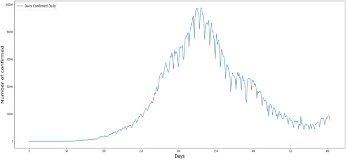
Per day statistics of daily confirmed cases.
Figure 2 shows per day statistics of deceased cases of COVID‐19.
FIGURE 2.
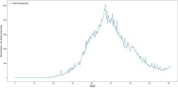
Per day statistics of daily deceased cases.
Figure 3 shows per day statistics of recovered cases of COVID‐19.
FIGURE 3.
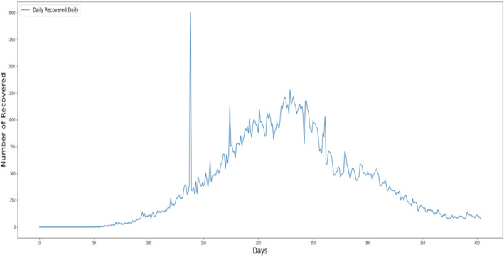
Per day statistics of daily recovered cases.
This collection contains data from India's states and union territories on a daily basis. The Ministry of Health and Family Welfare (MoHFW, 2022) (Willmott & Matsuura, 2005) provides data at the state level as shown in Figure 4.
FIGURE 4.
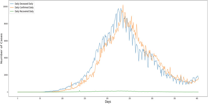
Statistical visualization for overall COVID‐19 cases
3.2. SARIMAX model
Box and Jenkin first proposed the SARIMAX model in 1976 (Box & Jenkins, 1976). SARIMAX is a time‐series data analysis statistical tool. To forecast the future values, the SARIMAX analyses the alterations between values in a time series. An SARIMAX model is made up of three elements. The Auto regression, integrated regression, and MA are abbreviated as AR, I, and M, respectively. As in (Hernandez‐Matamoros et al., 2020), every element is a parameter. Other models consist of the autoregressive (AR) model, the MA model, and the SARIMA model (Fattah et al., 2018). The dataset was tested via Augmented Dickey–Fuller (ADF) Test to see if it was stationary or not. To use the SARIMAX modelling approach effectively, the time series must be stationery and trend‐free. The ADF (Augmented Dickey–Fuller) approach was utilized to determine whether or not the time‐series data was stationary, including the log transformation and differences (Cheung & Lai, 1995). Table 3, shows the ADF and p‐value for the number of confirmed, recovered and deceased cases. The p‐value makes an inference whether series is stationary or not. The adfuller() function in statsmodels.tsa.stattools in the statsmodel package provides a reliable implementation of the ADF test.
TABLE 3.
ACF and PACF plot for various cases
| Stationary test | Daily confirmed cases | Daily recovered cases | Daily deceased cases |
|---|---|---|---|
| ADF Statistic | −2.946920 | −2.852354 | −3.322269 |
| p‐value | 0.040158 | 0.051176 | 0.013912 |
Figures 5, 6, 7 shows the stationary test have been performed on the dataset, on daily confirmed, recovered and deceased cases.
FIGURE 5.
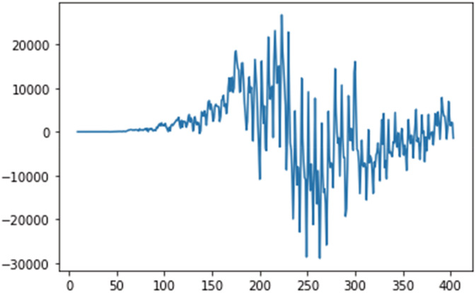
Stationary test for daily confirmed cases.
FIGURE 6.
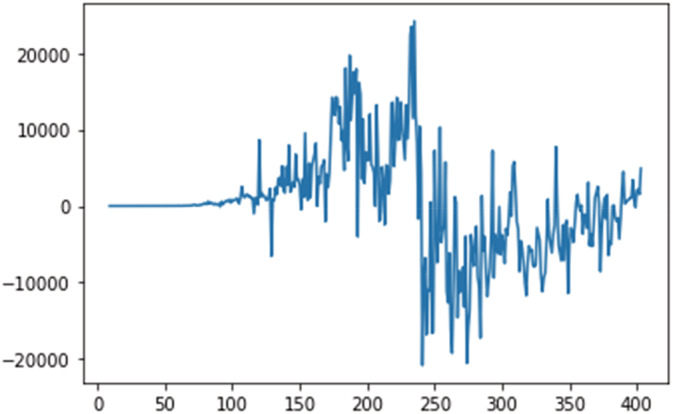
Stationary test for daily recovered cases.
FIGURE 7.
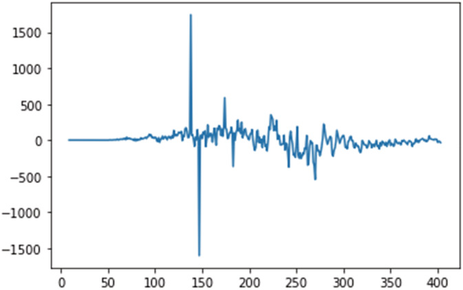
Stationary test for daily deceased cases.
The SARIMAX model's tuples are (p, q, r) × (P, Q, R, S) (Wei et al., 2016),
p: order of AR, d: rate of difference in trend, q: order of MA, P: seasonal AR lag value, D: rate of seasonal difference, Q: seasonal MA value and S: height of cyclical pattern.
Figure 8 shows the workflow of the proposed model optimizing the hyperparameters of SARIMAX through grid search cv.
FIGURE 8.
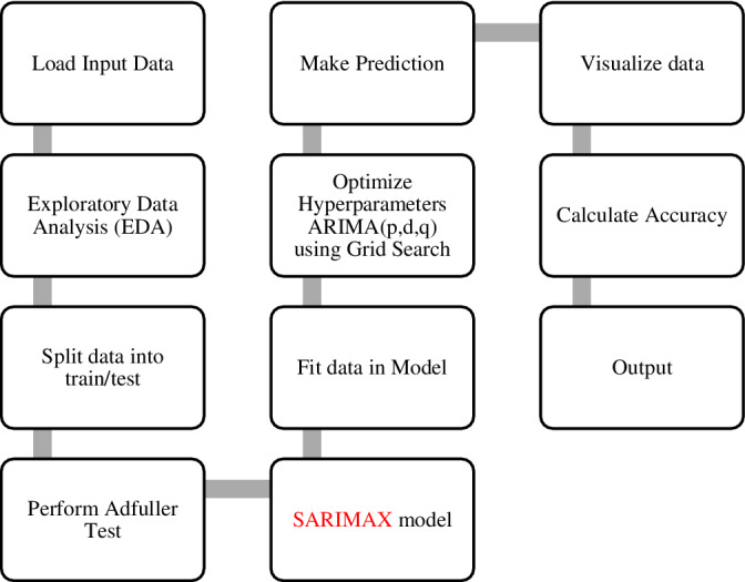
Workflow of the proposed optimized ARIMA model.
SARIMAX model is given by Equation (1) as mentioned below, (Prabhakaran, 2020)
| (1) |
where shows the first lag of the series, shows the second lag of the series and so on. shows the coefficient of first lag that the model examines, shows the coefficient of second lag that the model examines and so on. shows the intercept term examined by the model, is the output value which depends on its own lagged value and lagged predicted errors, and states the errors of the equations and so on.
AR MODEL
Auto regressive model is one where the value of depends only on its own lags, which is given by Equation (2) (Prabhakaran, 2020)
| (2) |
where shows the first lag of the series, shows the coefficient of the first lag that the model examines and shows the intercept term examined by the model.
MA MODEL.
Moving average is the model where the value depends only on the lagged predicted errors. This is given by Equation (3) below (Prabhakaran, 2020).
| (3) |
where and are the errors of Equations (4) and (5) as mentioned below
| (4) |
| (5) |
Prediction for daily confirmed cases in India Figures 9, 10, 11 show the prediction graphs for the confirmed cases, where the orange colour graph shows the prediction curve and the blue colour curve shows the original data points. The prediction results were obtained through the optimal SARIMAX (4, 1, 5)×(4, 1, 5, 9) by tuning the hyperparameters of the SARIMAX model to obtain the best order through grid search cv. Hyperparameter tuning is an optimization loop that is built on top of the machine learning model learning to categorize the collection of hyper parameters that results in the lowest validation set error. As a result, a validation set must be specified, as well as a loss (Bissuel, 2020).
FIGURE 9.
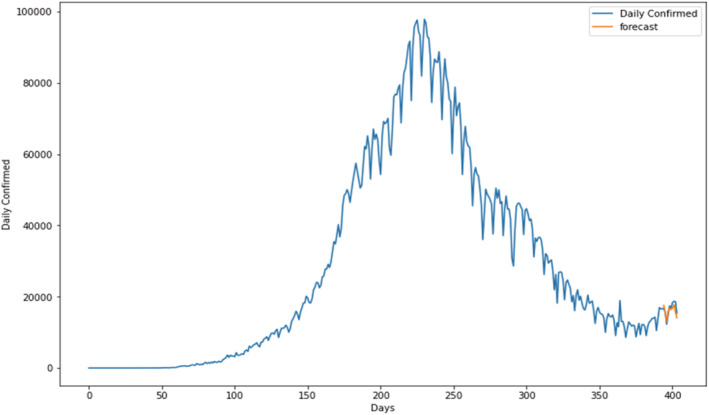
Prediction of daily confirmed cases using proposed SARIMAX with grid search CV model.
FIGURE 10.
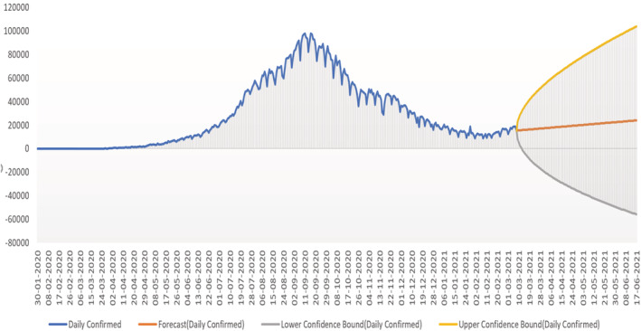
Prediction of daily confirmed cases using the SARIMAX with grid search CV model showing the upper and lower confidence bound.
FIGURE 11.
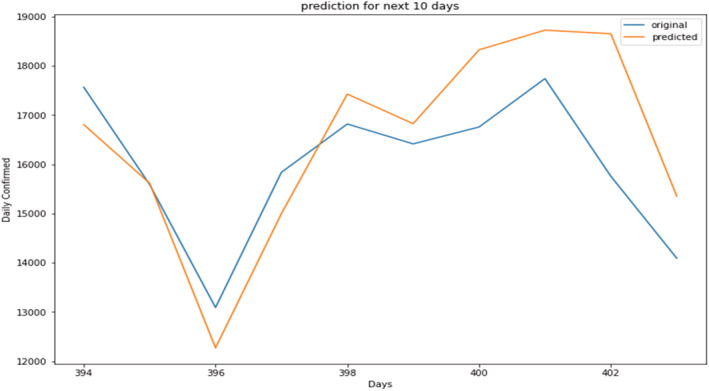
Prediction of daily confirmed cases (magnified view).
Table 4 shows the result of the SARIMAX optimized model for daily confirmed cases generated by the model.
-
b.
Prediction for daily recovered cases Figures 12, 13, 14, show the prediction graph for the recovered cases, where the orange colour graph shows the prediction curve and the blue colour curve shows the original data points. The prediction results were obtained through the optimal SARIMAX (5,1,1)×(5,1,1,9). Table 5, shows the result of the SARIMAX optimized model for daily recovered cases generated by the model.
-
c.
Prediction for daily deceased cases Figures 15, 16, 17, show the prediction graph for the deceased cases, where the orange colour graph shows the prediction curve and the blue colour curve shows the original data points. The prediction results were obtained through the optimal SARIMAX (5,1,1)×(5,1,1,9) through grid search cv by tuning the hyperparameters.
TABLE 4.
SARIMAX result summary for daily confirmed cases
| SARIMAX results | |||
|---|---|---|---|
| Dep. variable: | Daily confirmed | No. observations | 404 |
| Model | SARIMAX(4, 1, 5)×(4, 1, 5, 9) | Log likelihood | −3712.046 |
| Date | Fri, 22 Apr 2022 | AIC | 7462.091 |
| Time | 09:11:57 | BIC | 7537.642 |
| Sample | 0 | HQIC | 7492.028 |
| –404 | |||
| Covariance type | opg | ||
| coef | std err | z | P > |z| | [0.025 | 0.975] | |
|---|---|---|---|---|---|---|
| ar.L1 | 0.7939 | 0.030 | 26.502 | 0.000 | 0.735 | 0.853 |
| ar.L2 | −1.4358 | 0.032 | −45.423 | 0.000 | −1.498 | −1.374 |
| ar.L3 | 0.7950 | 0.032 | 24.933 | 0.000 | 0.732 | 0.857 |
| ar.L4 | −0.9865 | 0.025 | −39.866 | 0.000 | −1.035 | −0.938 |
| ma.L1 | −1.1329 | 0.114 | −9.898 | 0.000 | −1.357 | −0.909 |
| ma.L2 | 1.5383 | 0.168 | 9.152 | 0.000 | 1.209 | 1.868 |
| ma.L3 | −1.0728 | 0.237 | −4.518 | 0.000 | −1.538 | −0.607 |
| ma.L4 | 0.9236 | 0.189 | 4.894 | 0.000 | 0.554 | 1.294 |
| ma.L5 | −0.1590 | 0.148 | −1.073 | 0.283 | −0.449 | 0.131 |
| ar.S.L9 | 0.0702 | 1.302 | 0.054 | 0.957 | −2.482 | 2.622 |
| ar.S.L18 | −0.3919 | 1.072 | −0.365 | 0.715 | −2.494 | 1.710 |
| ar.S.L27 | −0.5440 | 0.822 | −0.662 | 0.508 | −2.156 | 1.067 |
| ar.S.L36 | 0.0223 | 0.958 | 0.023 | 0.981 | −1.855 | 1.900 |
| ma.S.L9 | −0.7236 | 1.282 | −0.564 | 0.572 | −3.236 | 1.789 |
| ma.S.L18 | 0.3973 | 1.558 | 0.255 | 0.799 | −2.656 | 3.451 |
| ma.S.L27 | 0.1201 | 1.426 | 0.084 | 0.933 | −2.674 | 2.914 |
| ma.S.L36 | −0.3731 | 1.268 | −0.294 | 0.769 | −2.858 | 2.112 |
| ma.S.L45 | −0.1721 | 0.751 | −0.229 | 0.819 | −1.644 | 1.299 |
| sigma2 | 1.681e+07 | 1.18e‐06 | 1.42e+13 | 0.000 | 1.68e+07 | 1.68e+07 |
| Ljung–Box (L1) (Q) | 3.76 | Jarque–Bera (JB) | 265.74 |
|---|---|---|---|
| Prob(Q) | 0.05 | Prob(JB) | 0.00 |
| Heteroskedasticity (H) | 40.89 | Skew | −0.84 |
| Prob(H) (two‐sided) | 0.00 | Kurtosis | 6.66 |
FIGURE 12.
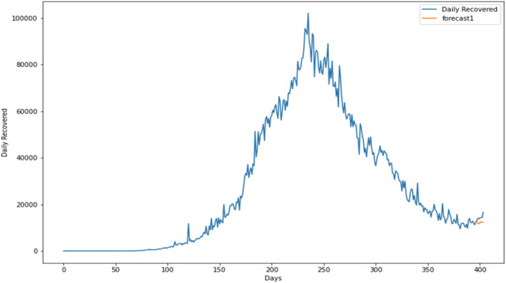
Prediction of daily recovered cases using the proposed SARIMAX with grid search CV model.
FIGURE 13.
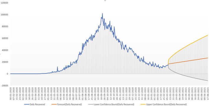
Prediction of daily recovered cases using the proposed SARIMAX with grid search CV model showing the upper and lower confidence bound.
FIGURE 14.
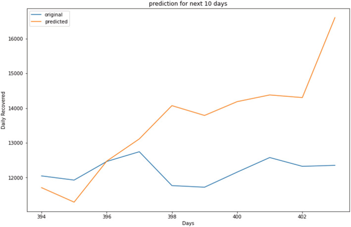
Prediction of daily recovered cases (magnified view).
TABLE 5.
SARIMAX results for daily recovered cases
| SARIMAX results | |||
|---|---|---|---|
| Dep. variable | Daily recovered | No. observations | 404 |
| Model | SARIMAX(5, 1, 1)×(5, 1, 1, 9) | Log‐likelihood | −3748.631 |
| Date | Wed, 27 Apr 2022 | AIC | 7523.262 |
| Time | 17:34:01 | BIC | 7574.955 |
| Sample | 0 | HQIC | 7543.745 |
| − 404 | |||
| Covariance Type: | opg | ||
| coef | std err | z | P > |z| | [0.025 | 0.975] | |
|---|---|---|---|---|---|---|
| ar.L1 | −1.5075 | 0.040 | −37.374 | 0.000 | −1.587 | −1.428 |
| ar.L2 | −0.7813 | 0.065 | −11.931 | 0.000 | −0.910 | −0.653 |
| ar.L3 | −0.3513 | 0.081 | −4.343 | 0.000 | −0.510 | −0.193 |
| ar.L4 | −0.1132 | 0.074 | −1.527 | 0.127 | −0.259 | 0.032 |
| ar.L5 | −0.0015 | 0.038 | −0.040 | 0.968 | −0.077 | 0.074 |
| ma.L1 | 0.9776 | 0.019 | 50.572 | 0.000 | 0.940 | 1.016 |
| ar.S.L9 | 0.0068 | 0.041 | 0.165 | 0.869 | −0.074 | 0.088 |
| ar.S.L18 | 0.0964 | 0.045 | 2.126 | 0.033 | 0.008 | 0.185 |
| ar.S.L27 | 0.0731 | 0.041 | 1.764 | 0.078 | −0.008 | 0.154 |
| ar.S.L36 | 0.0183 | 0.052 | 0.349 | 0.727 | −0.084 | 0.121 |
| ar.S.L45 | 0.0459 | 0.045 | 1.028 | 0.304 | −0.042 | 0.133 |
| ma.S.L9 | −0.9985 | 0.045 | −22.062 | 0.000 | −1.087 | −0.910 |
| sigma2 | 1.023e+07 | 4.54e‐09 | 2.25e+15 | 0.000 | 1.02e+07 | 1.02e+07 |
| Ljung–Box (L1) (Q) | 0.00 | Jarque–Bera (JB) | 317.69 |
|---|---|---|---|
| Prob(Q) | 0.99 | Prob(JB) | 0.00 |
| Heteroskedasticity (H) | 8.58 | Skew | −0.07 |
| Prob(H) (two‐sided) | 0.00 | Kurtosis | 7.40 |
FIGURE 15.
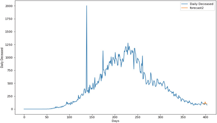
Prediction of daily deceased cases using the proposed SARIMAX with the grid search CV model.
FIGURE 16.
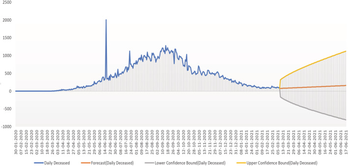
Prediction of daily deceased cases using the proposed SARIMAX with grid search CV showing the upper and lower confidence boundary.
FIGURE 17.
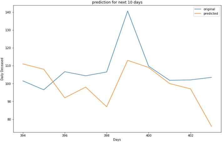
Prediction of daily deceased cases (magnified view).
Table 6 shows the result of SARIMAX optimized model for daily deceased cases generated by the model.
-
d.
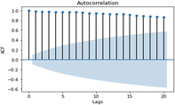
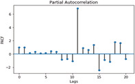
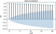
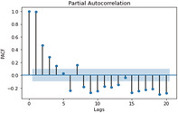
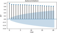
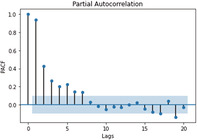
ACF and PACF graphs for cases For the ARIMA model parameters, an ACF (auto‐correlation function) graph and PACF (partial autocorrelation) correlogram were constructed. In a timeseries, the association between present observation with the past time‐steps or lags observation. Autocorrelation function (ACF), the plot of autocorrelation versus the lags is called autocorrelation plot. Hence, ACF illustrates the linear relation between the assumption at ‘t’ time and observation at the past time ‘t−k’ (ArunKumar et al., 2021). ACF assists researchers in classifying knowledge linked to the previous concurrent finding. The partial ACF is used to determine the level of interface between observations made between two‐time intervals of elimination. PACF aids in determining the degree of correctness of the current variables using its preceding values, while maintaining specified constant values (Makridakis et al., 2008). The ACF and PACF plots are shown in Table 7,
TABLE 6.
SARIMAX results for daily deceased cases
| SARIMAX results | |||
|---|---|---|---|
| Dep. variable | Daily deceased | No. observations | 404 |
| Model | SARIMAX(5, 1, 1)×(5, 1, 1, 9) | Log‐likelihood | −2406.326 |
| Date | Wed, 27 Apr 2022 | AIC | 4838.652 |
| Time | 17:34:39 | BIC | 4890.345 |
| Sample | 0 | HQIC | 4859.135 |
| −404 | |||
| Covariance type | opg | ||
| coef | std err | z | P > |z| | [0.025 | 0.975] | |
|---|---|---|---|---|---|---|
| ar.L1 | −0.1998 | 0.158 | −1.266 | 0.206 | −0.509 | 0.110 |
| ar.L2 | −0.1968 | 0.111 | −1.770 | 0.077 | −0.415 | 0.021 |
| ar.L3 | −0.1796 | 0.079 | −2.283 | 0.022 | −0.334 | −0.025 |
| ar.L4 | −0.1434 | 0.063 | −2.286 | 0.022 | −0.266 | −0.020 |
| ar.L5 | −0.0235 | 0.048 | −0.489 | 0.625 | −0.118 | 0.071 |
| ma.L1 | −0.5226 | 0.156 | −3.345 | 0.001 | −0.829 | −0.216 |
| ar.S.L9 | 0.0241 | 0.045 | 0.540 | 0.589 | −0.063 | 0.111 |
| ar.S.L18 | 0.0977 | 0.066 | 1.485 | 0.138 | −0.031 | 0.227 |
| ar.S.L27 | 0.0358 | 0.057 | 0.631 | 0.528 | −0.075 | 0.147 |
| ar.S.L36 | 0.2037 | 0.076 | 2.669 | 0.008 | 0.054 | 0.353 |
| ar.S.L45 | −0.0597 | 0.109 | −0.545 | 0.585 | −0.274 | 0.155 |
| ma.S.L9 | −0.9999 | 0.015 | −67.339 | 0.000 | −1.029 | −0.971 |
| sigma2 | 1.092e+04 | 1.36e‐06 | 8.02e+09 | 0.000 | 1.09e+04 | 1.09e+04 |
| Ljung–Box (L1) (Q) | 0.01 | Jarque–Bera (JB) | 313532.18 |
|---|---|---|---|
| Prob(Q) | 0.93 | Prob(JB) | 0.00 |
| Heteroskedasticity (H) | 0.07 | Skew | 8.58 |
| Prob(H) (two‐sided) | 0.00 | Kurtosis | 140.13 |
TABLE 7.
ACF and PACF plot for various cases
| ACF GRAPH (lag = 20) | PACF GRAPH (lag = 20) | |
|---|---|---|
| Confirmed cases |
ACF Graph for confirmed cases |
PACF Graph for confirmed cases |
| Deceased cases |
ACF graph for deceased cases |
PACF graph for deceased cases |
| Recovered cases |
ACF graph for recovered cases |
PACF graph for recovered cases |
The formula (Nayak et al., 2019),
| (6) |
where k is the lag, provides the difference between and . Lag k autocorrelation indicate the association between the assumptions that are k time periods separated or aside.
Partial autocorrelation function (PACF), the intervening observations are focused while computing the association between the two assumptions at distinct times represents the time series. So, PACF between the two observations, say and can be shown in the equation below (ArunKumar et al., 2021).
| (7) |
In Table 7 (see inline figures) the light blue colour indicates the values over which the autocorrelations are statistically significantly different from zero. In simple words, it describes how strongly the series' current value is connected to its previous values. Because ACF incorporates all of these factors while determining correlations, it is referred as a ‘full auto‐correlation plot’. We can predict a progressive decline in the ACF plot because the present has a good association with the previous lags. We expect PACF to drop sharply after close lags because these lags can record variation so well that we do not require previous lags to forecast present (Salvi, 2019)
-
e.
SARIMAX optimized model validation For hyperparameter selection in model, grid search approach is used. Minor changes in hyperparameter values can result in significantly different forecast results, selecting great hyperparameter values is crucial. Grid search is a strategy for determining the best hyperparameters for a model. Finding hyperparameters in training data, unlike parameters, is impossible. As a result, we develop a model for each combination of hyperparameters in order to determine the best hyperparameters. Cross‐validation assesses how well a model generalizes to a new dataset. To acquire a good approximation of how well a predictive model performs, cross‐validation is performed. We have two datasets with this method: an independent dataset and a training dataset. We can divide a single dataset into two sets by partitioning it. GridSearchCV has two methods: ‘fit’ and ‘score’ (Ayuya, 2021).
Figure 18 shows the proposed workflow for optimizing the SARIMAX model using grid search cv.
FIGURE 18.

SARIMAX model optimization using the grid search cv.
Algorithm for SARIMAX model using grid search approach :
-
Define
ts: Time Series Data
pdq: parameters of ARIMA model
pdqs: seasonal ARIMA parameters
maxiter: no. of iterations
frequency: bydefault=’M' for month
Initialize an array fore[]
-
For parameters in pdqs
mod = sm.tsa.statespace.SARIMAX(ts, order = pdq, seasonal_order = pdqs, enforce_stationarity = False,
enforce_invertibility = False, freq = freq)
output = mod. fit()
fore. append([pdq, pdqs, output.bic])
-
Convert into dataframes and then sort as well as return top 9 combinations. Finally apply grid search function to SARIMAX model
Forecast_df = fore_df.sort_values(by = [‘bic’],ascending = True)[0:9]
return Forecst_df
sarimax_gridsearch(ts, pdq, pdqs, freq = ‘M')
4. DATA VALIDATION
The disparities between the raw series observed and the anticipated values derived from the two techniques were compared to demonstrate the efficacy of the prediction strategy utilized in this investigation. Because the combined and chosen estimates for measuring bias and model accuracy as analytical approaches have been widely used, the R‐Square and root‐mean‐square error (RMSE) were chosen as measurements (Christodoulos et al., 2011). The model is validated using the performance metrics as mentioned in Table 8,
TABLE 8.
Evaluation metrics
| Measure | Formula | Remarks | ||
|---|---|---|---|---|
|
|
|
R‐Square score tells how close the forecasted value is to the regression line (Chordia & Pawar, 2021). The R‐squared (R 2) score is a simple to compute and explain gauge of confidence (Lupón & Gaggin, 2015). It is the level to which a data point fits the linear regression, thereby indicating how well the regression line forecasts real values. The coefficient of determination gives you to compute how much variance the model's self‐standing variables have displayed. It gives us the model's goodness‐of‐fit, as well as a score that is always between 0 and 1 (Renaud & Victoria‐Feser, 2010). Whereas the true value at certain ith assumption, is the forecasted value at ith assumptions, shows the mean of the overall observations, and is the overall count of observations | ||
| RMSE |
RMSE = |
RMSE is defined as the variance or root of the residuals. It's a metric for how the residuals distribute around the best‐fit line. It will be easy to read because the units are the same as the output units. This is often negative in nature, and a lower RMSE value enhances model performance. Whereas shows the predicted value, shows the real value and n is the count of observations. (Moody, 2019; Willmott & Matsuura, 2005) |
4.1. Monte Carlo simulation
Monte‐Carlo sampling is a prominent tool for comparing the forecasting algorithms' performance. Multiple patches of a dataset are randomly picked in this procedure, and then tests of the forecasting systems' performance are run. It gives you the average of the error numbers you got for each data patch. The Monte‐Carlo strategy's most remarkable feature is that it ensures an accurate comparison of forecasting systems and eliminates the possibility of skewed findings acquired by chance (Bokde et al., 2020).
Monte Carlo Simulation (Davies et al., 2014) are provided below.
Step 1: For each input random variable, define a distribution of possible inputs.
Step 2: Create random outputs from those distributions.
Step 3: Use that set of outputs to do a deterministic calculation.
Step 4: Combine the results of the separate computations to arrive at a final result.
Syntax: monte_carlo(object, size, iteration, fval = 0, figs = 0).
Where, the parameter object indicates the output of prediction error function. Size shows the quantity of time series data used in the strategy. Iteration represents the number of iterations performed. The fval shows the flag to view predicted values in each iteration. Finally, figs shows the flag to display the plots for each iteration.
5. RESULTS
Results obtained through the optimal SARIMAX model have shown a great improvement in the performance, tuning the hyperparameters through grid search cv accessing the best parameter for the SARIMAX model, which also improves the performance. Hence, the parameters (p, d, q)×(P,D,Q,S) can be optimally obtained. The ‘event’ description and the data collection method, employed in the present case, determine the outcome of the prediction and estimation. Case definition and data gathering was preserved in real time for the future comparisons or viewpoints. In general, the fitted values and predicted values, produced using two methods (R2, RMSE), came quite close to the real incidence of COVID‐19 disorders. Although more data is needed to provide a more precise forecast, the virus's transmission looks to be significantly decreasing. Furthermore, despite the fact that the number of confirmed cases continues to rise, the frequency has decreased significantly. The number of cases will hit an all‐time high if the virus does not evolve any new mutations. Figures 19, 20, 21 show the residual error plots for predicting daily confirmed, recovered and deceased cases.
FIGURE 19.
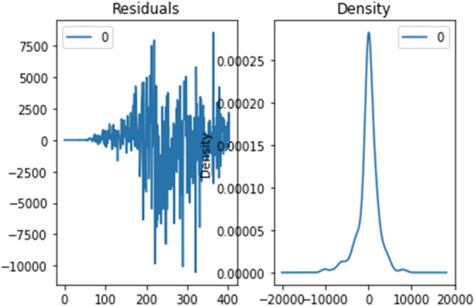
Residual error for predicting daily confirmed cases using the SARIMAX optimized model.
FIGURE 20.
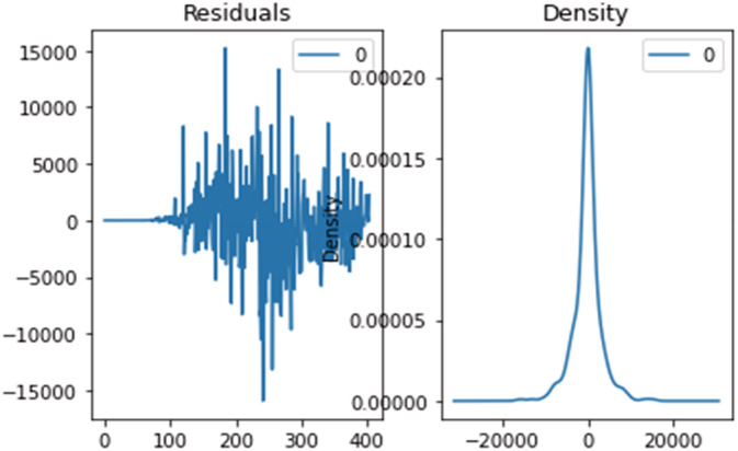
Residual error for predicting daily recovered cases using the SARIMAX optimized model.
FIGURE 21.
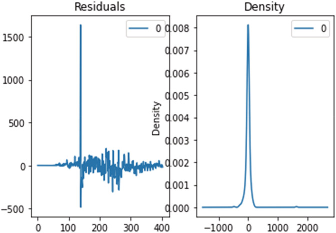
Residual error for predicting daily deceased cases using the SARIMAX optimized model.
The comparison has been made with other models showing the forecast for the 30‐day time period, the metrics obtained are shown in Tables 9 using the proposed SARIMAX model,
TABLE 9.
Evaluation metrics showing comparison with various state‐of‐art models
| Performance metrics | Linear regression | Polynomial regression | Prophet | SARIMAX (without grid search) | SARIMAX (with grid search) |
|---|---|---|---|---|---|
| R Square | 0.01 | 0.31 | 0.46 | 0.255946 | 0.5112 |
| RMSE | 284809.4 | 149117.8 | 568.58 | 3122.8080 | 1251 |
Table 5 shows the comparison of various state‐of‐art models with the proposed model. The comparison shows that our model is performing better in terms of minimum loss. The SARIMAX model with a grid search approach is producing better results as compared to SARIMAX without a grid search approach. This table shows the performance metrics of confirmed cases in India. The findings are correct, with a steady rise in the number of confirmed and deceased cases and a falling graph for recovered cases.
The Monte Carlo() function extends the prediction errors() module by allowing you to evaluate different approaches for randomly selected patches of the input time series Table 10 shows the results obtained through Monte Carlo using various models.
TABLE 10.
Monte Carlo simulation for various models
| Iterations | SARIMAX (with grid search) | Linear regression | Polynomial regression | Prophet | SARIMAX (without grid search) |
|---|---|---|---|---|---|
| #23 | 1.2509 | 4.2372 | 2.4512 | 3.5612 | 1.2569 |
| #11 | 2.3710 | 7.9825 | 3.1298 | 2.8720 | 2.8719 |
| #45 | 1.5420 | 4.9146 | 2.8713 | 3.4101 | 2.8712 |
| #99 | 1.9812 | 5.7612 | 4.7512 | 2.3163 | 1.7610 |
| #78 | 2.7681 | 3.7123 | 3.1210 | 2.8731 | 2.8790 |
| #2 | 2.6501 | 4.9812 | 5.1291 | 2.5672 | 2.9854 |
| #61 | 3.7912 | 3.1240 | 4.1209 | 3.7612 | 2.0915 |
| #12 | 1.8721 | 5.1271 | 5.1971 | 3.8756 | 1.7609 |
| #55 | 1.9632 | 7.5621 | 4.1263 | 2.6732 | 3.9650 |
| #86 | 1.7621 | 8.8291 | 3.6101 | 3.5412 | 3.8912 |
| Mean | 2.1951 | 5.62313 | 3.8508 | 3.14511 | 2.6334 |
6. CONCLUSION
In this paper, prediction of confirmed, recovered, and deceased Indian cases of COVID‐19 obtained for 20 days in advance, until 29 March 2021, using an optimized SARIMAX statistical model with grid search cross validation approach. This study answers two of today's most pressing questions; namely when the COVID‐19 epidemic would cease, and would there a chance of a second rebound if people resumed their normal lives. Despite fast viral mutation and the structure of the dataset dependent on time and date, the research attempted to limit data variability by using just the dataset. Predicted results are more accurate with usage of the optimal SARIMAX model. Our forecast indicates that the count of confirmed as well as deceased cases are higher, whereas recovered cases prediction shows a decreasing trend. Proposed model can be extended to predict the cases using longer dataset. Furthermore, a hybrid model can be created incorporating proposed model. On the basics of our predictions, strategy administrators of healthcare should take necessary decisions at the right time in providing healthcare aids to the public as well as the agencies responsible for transporting equipment to hospitals. The prediction would also help the policymakers to frame their policies based on the pandemic situation. The result presented in this article emphasizes the significance of societal distancing and execution of various protective ways of COVID‐19.
Biographies
Sweeti Sah is a full time Ph.D., research scholar (Institute fellowship category) in the Department of Computer Science and Engineering at National Institute of Technology Puducherry, Karaikal – 609609, India. She has completed her bachelor in CSE from Ambalika Institute of Management and Technology, Lucknow, U.P. (Affiliated to Uttar Pradesh Technical University) and master degree in CSE from Babasaheb Bhimrao Ambedkar University (A Central University), Lucknow, U.P., India. She is M.Tech Gold Medalist. She is GATE (CSE) and NET (Computer Applications) qualified. Her research interest includes Machine Learning and Deep Learning.
Dr. Balasubramanian Surendiran is working as an Associate Professor (CSE Department)NIT Puducherry, India. He had published more than 35 papers in various international journal and conferences. His research interest includes medical imaging, machine learning and dimensionality reduction.
Dr. Ramasamy Dhanalaxmi is working as an Associate Professor and Head of Department (CSE Department) in IIIT Tiruchirapalli, India. Her research interest includes medical imaging, machine learning and networks.
Professor Mohammad Yamin is the Director of the Social Responsibility and Community Service unit of the faculty of Economics and Administration of the King Abdulaziz University (KAU), Jeddah, Saudi Arabia. Professor Mohammad Yamin holds a PhD degree from the Australian National University, ranked in the top twenty universities of the word and is number one Australian universities according to QS World University Rankings 2017. Dr Yamin is a full professor of MIS at the king Abdulaziz University in Jeddah, Saudi Arabia, and an Adjunct at the College of Computer Science of the Australian National University.
Sah, S. , Surendiran, B. , Dhanalakshmi, R. , & Yamin, M. (2022). Covid‐19 cases prediction using SARIMAX Model by tuning hyperparameter through grid search cross‐validation approach. Expert Systems, e13086. 10.1111/exsy.13086
DATA AVAILABILITY STATEMENT
The data that support the findings of this study are available from the corresponding author upon reasonable request.
REFERENCES
- Almutairi, M. M. , Yamin, M. , Halikias, G. , & Abi Sen, A. A. (2021). A framework for crowd management during COVID‐19 with artificial intelligence. Sustainability, 14, 303. 10.3390/su1401030 [DOI] [Google Scholar]
- Andrea, R. , & Giuseppe, R. (2020). COVID‐19 and Italy: What next? The Lancet 395, 395(10231), 1225–1228. [DOI] [PMC free article] [PubMed] [Google Scholar]
- ArunKumar, K. E. , Kalaga, D. V. , Sai Kumar, C. M. , Chilkoor, G. , Kawaji, M. , & Brenza, T. M. (2021). Forecasting the dynamics of cumulative COVID‐19 cases (confirmed, recovered and deaths) for top‐16 countries using statistical machine learning models: Auto‐regressive integrated moving average (ARIMA) and seasonal auto‐regressive integrated moving average (SARIMA). Applied Soft Computing, 103, 107161. [DOI] [PMC free article] [PubMed] [Google Scholar]
- Ayuya, C. 2021. Using grid search to optimize hyper parameters. https://www.section.io/engineering-education/grid-search/#grid-search
- Benvenuto, D. , Giovanetti, M. , Vassallo, L. , Angeletti, S. , & Ciccozzi, M. (2020). Application of the ARIMA model on the COVID‐2019 epidemic dataset. Data in Brief, 29, 105340. [DOI] [PMC free article] [PubMed] [Google Scholar]
- Bissuel, A. 2020. Hyper‐parameter optimization algorithms: a short review. https://medium. com/criteo‐labs/hyper‐parameter‐optimizationalgorithms‐2fe447525903
- Bokde, N. , Dhanraj, Z. , Yaseen, M. , & Andersen, G. B. (2020). ForecastTB—an R package as a test‐bench for time series forecasting—application of wind speed and solar radiation modeling. Energies, 13(10), 1–24. [Google Scholar]
- Box, G. E. , & Jenkins, G. M. (1976). Time series analysis: Forecasting and control (Revised ed.). Holden‐Day. [Google Scholar]
- Cao, W. , Fang, Z. , Hou, G. , Han, M. , Xu, X. , Dong, J. , & Zheng, J. (2020). The psychological impact of the COVID‐19 epidemic on college students in China. Psychiatry Research, 287, 112934. [DOI] [PMC free article] [PubMed] [Google Scholar]
- Cheung, Y.‐W. , & Lai, K. S. (1995). Lag order and critical values of the augmented Dickey–Fuller test. Journal of Business & Economic Statistics, 13(3), 277–280. [Google Scholar]
- Chordia, S. , & Pawar, Y. 2021. Analyzing and Forecasting COVID‐19 Outbreak in India. 11th International Conference on Cloud Computing, Data Science & Engineering (Confluence), IEEE, pp. 1059–1066.
- Christodoulos, C. , Michalakelis, C. , & Varoutas, D. (2011). On the combination of exponential smoothing and diffusion forecasts: An application to broadband diffusion in the OECD area. Technological Forecasting and Social Change, 78(1), 163–170. [Google Scholar]
- Davies, R. , Coole, T. , & Osipyw, D. (2014). The application of time series modelling and Monte Carlo simulation: Forecasting volatile inventory requirements. Applied Mathematics, 05, 1152–1168. [Google Scholar]
- Duan, X. , & Zhang, X. (2020). ARIMA modelling and forecasting of irregularly patterned COVID‐19 outbreaks using Japanese and south Korean data. Data in Brief, 31, 105779. [DOI] [PMC free article] [PubMed] [Google Scholar]
- Fanelli, D. , & Piazza, F. (2020). Analysis and forecast of COVID‐19 spreading in China, Italy and France. Chaos, Solitons & Fractals, 134, 109761. [DOI] [PMC free article] [PubMed] [Google Scholar]
- Fanoodi, B. , Malmir, B. , & Jahantigh, F. F. (2019). Reducing demand uncertainty in the platelet supply chain through artificial neural networks and ARIMA models. Compute. Biol. Med., 113, 1–10. [DOI] [PubMed] [Google Scholar]
- Fattah, J. , Ezzine, L. , Aman, Z. , El Moussami, H. , & Lachhab, A. (2018). Forecasting of demand using ARIMA model. International Journal of Engineering Business Management, 10, 1–9. [Google Scholar]
- Gecili, E. , Ziady, A. , & Szczesniak, R. D. (2021). Forecasting COVID‐19 confirmed cases, deaths and recoveries: Revisiting established time series modeling through novel applications for the USA and Italy. PloS one, 16(1), 1–11. [DOI] [PMC free article] [PubMed] [Google Scholar]
- Hernandez‐Matamoros, A. , Fujita, H. , Hayashi, T. , & Perez‐Meana, H. (2020). Forecasting of COVID19 per regions using ARIMA models and polynomial functions. Applied Soft Computing, 96, 106610. [DOI] [PMC free article] [PubMed] [Google Scholar]
- Ho, C. S. , Chee, C. Y. , & Ho, R. C. (2020). Mental health strategies to combat the psychological impact of covid‐19 beyond paranoia and panic. Annals of the Academy of Medicine, Singapore, 49(1), 1–3. [PubMed] [Google Scholar]
- Kaggle . 2021. COVID‐19 in India. Retrieved March 9, 2021, from https://www.kaggle.com/sudalairajkumar/covid19-in-india?select=covid_19_india.csv
- Khan, F. M. , & Gupta, R. (2020). Arima and nar based prediction model for time series analysis of covid‐19 cases in India. Journal of Safety Science and Resilience, 1(1), 12–18. [Google Scholar]
- Makridakis, S. , Wheelwright, S. C. , & Hyndman, R. J. (2008). Forecasting methods and applications. Wiley. [Google Scholar]
- Moody, J. What does RMSE really mean, Sep 6, 2019. https://towardsdatascience.com/what-does-rmse-really-mean-806b65f2e48e
- Nayak, M. S. , Prasad, D. , & Narayan, K. A. (2019). Forecasting dengue fever incidence using ARIMA analysis. International Journal of Collaborative Research on Internal Medicine & Public Health, 11(3), 924–932. [Google Scholar]
- Prabhakaran, S . 2020. ARIMA Model–Complete Guide to Time Series Forecasting in Python Machine Learning Plus. Retrieved 29 March 2020, from https://www.machinelearningplus.com/time-series/arima-model-time-seriesforecasting-python/
- Rao, C. R. , & Gudivada, V. N. (2018). Computational analysis and understanding of natural languages: Principles. Methods and Applications, 38, 197–226. [Google Scholar]
- Renaud, O. , & Victoria‐Feser, M.‐P. (2010). A robust coefficient of determination for regression. Journal of Statistical Planning and Inference, 140(7), 1852–1862. [Google Scholar]
- Salvi, J. (2019). Significance of ACF and PACF plots in time series analysis. Towards Data Science, 27. https://towardsdatascience.com/significance-of-acf-and-pacf-plots-in-time-series-analysis-2fa11a5d10a8 [Google Scholar]
- Singh, S. , Parmar, K. S. , Kumar, J. , Jitendra, S. , & Makkhan, S. (2020). Development of new hybrid model of discrete wavelet decomposition and autoregressive integrated moving average (ARIMA) models in application to one month forecast the casualties cases of COVID‐19. Chaos, Solitons & Fractal, 135, 1–9. [DOI] [PMC free article] [PubMed] [Google Scholar]
- Wei, W. , Jiang, J. , Liang, H. , Gao, L. , Liang, B. , Huang, J. , et al. (2016). Application of a combined model with autoregressive integrated moving average (ARIMA) and generalized regression neural network (GRNN) in forecasting hepatitis incidence in Heng County. China. PloS one, 11(6), 1–13. [DOI] [PMC free article] [PubMed] [Google Scholar]
- Willmott, C. J. , & Matsuura, K. (2005). Advantages of the mean absolute error (MAE) over the root mean square error (RMSE) in assessing average model performance. Climate Research, 30(1), 79–82. [Google Scholar]
- Woo, P. C. , Huang, Y. , Lau, S. K. , & Yuen, K. Y. (2010). Coronavirus genomics and bioinformatics analysis. Viruses, 2(8), 1804–1820. [DOI] [PMC free article] [PubMed] [Google Scholar]
- Yamin, M. (2020). Counting the cost of COVID‐19. International Journal of Information Technology, 12(2), 311–317. 10.1007/s41870-020-00466-0 [DOI] [PMC free article] [PubMed] [Google Scholar]
Associated Data
This section collects any data citations, data availability statements, or supplementary materials included in this article.
Data Availability Statement
The data that support the findings of this study are available from the corresponding author upon reasonable request.


