A Generative Approach to Materials Discovery, Design, and Optimization

Abstract

Despite its potential to transform society, materials research suffers from a major drawback: its long research timeline. Recently, machine-learning techniques have emerged as a viable solution to this drawback and have shown accuracies comparable to other computational techniques like density functional theory (DFT) at a fraction of the computational time. One particular class of machine-learning models, known as “generative models”, is of particular interest owing to its ability to approximate high-dimensional probability distribution functions, which in turn can be used to generate novel data such as molecular structures by sampling these approximated probability distribution functions. This review article aims to provide an in-depth understanding of the underlying mathematical principles of popular generative models such as recurrent neural networks, variational autoencoders, and generative adversarial networks and discuss their state-of-the-art applications in the domains of biomaterials and organic drug-like materials, energy materials, and structural materials. Here, we discuss a broad range of applications of these models spanning from the discovery of drugs that treat cancer to finding the first room-temperature superconductor and from the discovery and optimization of battery and photovoltaic materials to the optimization of high-entropy alloys. We conclude by presenting a brief outlook of the major challenges that lie ahead for the mainstream usage of these models for materials research.

1. Introduction

Materials have played a crucial role in the evolution of technology through the ages, as is evidenced by historical epochs being named after the most advanced material of the era, from the Stone Age, to the Iron and Bronze Ages, to the current Silicon and Composite Nanomaterials Ages.^1,2 Materials research, however, has a fundamental drawback: the timeline associated with it is very high, and the probability of success is very low, dissuading many potential investors from investing in materials research.³ The cyclic process of experimentation, characterization, and optimization is highly inefficient and time consuming, extending the timeline of materials discovery to 10–20 years, with many modern-day advanced materials like lithium-ion batteries and fuel cells being developed in a time frame of 20–25 years (refer to Figure 1a).^3,4 Modern-day materials research and development can be broken down into seven discrete time-consuming stages from discovery to deployment, with each stage in principle being completed by a different team of engineers or scientists, compounding to the complexity (refer to Figure 1b).⁵ The complexity of materials research is further amplified by the sheer vastness of the chemical space which can be visualized as being “analogous to the cosmological universe in its vastness, with chemical compounds populating space instead of stars”.⁶ A very small fraction of the chemical space has been explored to date for the development of advanced materials. The fact remains that a vast majority of this space, estimated to be in excess of 10⁶⁰, the total number of chemically feasible, carbon-based molecules, remains unexplored.^7,8

Figure 1.

(a) Selected examples of timelines of the development of modern-day advanced materials versus the expectations of investors and typical development capacities. Reprinted with permission from ref (3). Copyright 2018 Elsevier. (b) The conventional seven-stage materials discovery, development, and optimization process, with each stage having complexities associated with it, making the overall process very time-consuming. Inspired from ref (5).

This motivates a venture into the development of tools to explore the largely unknown chemical space using computational techniques. These computational techniques are developed to facilitate a focused experimental effort in targeted and confined regimes, leading to faster research timelines.^3,9 A very commonly used computational technique in the modern-day materials discovery process is virtual screening (VS), which is used to reduce a large number of target materials to a smaller number using computational algorithms. These smaller number of molecules are then screened and analyzed using high-throughput techniques.¹⁰⁻¹³ While powerful algorithms make it feasible to screen close to 100 000 compounds/day, high-throughput techniques are limited by very low hit rates (≈1%).^14,15 Owing to this, techniques such as de novo materials design were developed, where novel chemical structures that are not present in standard chemical databases are assembled from scratch.^9,16 Popular de novo algorithms include structure-based algorithms such as LEGEND¹⁷ and SPROUT¹⁸ and evolutionary algorithms such as MEGA¹⁹ and TOPAS.²⁰ Other popular computational techniques that are used for predicting the properties of materials include density functional theory (DFT) that deals with electronic interactions²¹ and molecular dynamics (MD) that deals with atomic interactions.²²

Over the years, due to the generation and availability of massive data sets and the increase in computational power, there has been a meteoric rise in the employment of machine-learning algorithms.²³ While well established in areas such as image analysis and face recognition,²⁴ machine learning is being increasingly applied in the drug-discovery^25,26 and material property prediction pipelines, actively replacing the more conventional computational algorithms discussed above. The inversion of these structure–property prediction machine-learning algorithms can be used to generate novel molecules. A fairly new class of machine-learning models called “generative models” have come along as promising candidates for tackling this inversion problem. Generative models are trained to approximate high-dimensional probability distribution functions, which in turn can be used to generate novel data by sampling these approximated probability distribution functions.^27,28 An example of this is pioneering work by Gomez-Bombarelli et al.,²⁹ where a class of generative models known as variational autoencoders (VAE) were trained to convert a discrete data representation (a set of molecules) to a continuous representation, which was then again converted to a discrete representation. In the process, the continuous representation was sampled to generate novel data (in this case, novel molecules). Both VAEs and the work by Gomez-Bombarelli et al. have been discussed in detail in later sections.

While machine learning in materials science has been the subject of several excellent review articles,³⁰⁻³⁴ the focus has been more on conventional machine-learning and deep-learning algorithms and their applications and less on the principles of generative modeling. The underlying principles and mathematics of generative models are not trivial, and in order to understand their applications, an understanding of the mathematics is crucial. This article, thus, aims to provide a comprehensive understanding of the underlying principles of three classes of generative models: recurrent neural networks (RNNs), variational autoencoders (VAEs), and generative adversarial networks (GANs), with respect to applications pertaining to materials discovery. We then proceed to review the progress of these models in the domains of biomaterials and organic drug-like materials, energy materials, and structural materials. Finally, we offer insights into the major challenges involved in the application of generative models in materials science and highlight possible directions for the way forward, for a more efficient materials discovery, design, and optimization.

2. Underlying Principles of the Generative Approach

The first step in the conventional approach to materials discovery or any broad domain in engineering involves the accumulation of vast amounts of domain knowledge which is very time consuming and tedious. A machine-learning approach is able to replace this with the relatively simpler task of collecting vast amounts of data.³⁵ These data are often referred to as the “training set” and are leveraged to train machine-learning algorithms. Machine-learning algorithms can be broadly classified into three categories: supervised learning, unsupervised learning, and reinforcement learning.^23,35,36

Supervised machine learning can be conceptualized as a search for algorithms that make use of externally supplied instances of data to infer hypotheses, which in turn can be used to make future predictions on unseen instances of data.³⁷ Simply put, supervised machine learning involves the search for functions that map a known set of input variables to desired output variables. A “supervisor” instructs the system to associate input variables to desirable outputs.^36,38 Once this mapping is complete, unseen data can be fed into these functions as input, leading to the generation of predictions as output. From a materials perspective, supervised learning techniques are used mainly for the prediction of materials properties and the screening of large databases.

Considering the statistical framework of a supervised machine-learning algorithm, the input to the algorithm, known as the “training data set”, is a finite sequence S = ((x₁, y₁), ..., (x_n, y_n)) in the (X × Y)ⁿ space, with x_i ∈ X and y_i ∈ Y.^38,39 This form of data is known as labeled data, as for each input x_i there is a labeled output y_i. The output of this algorithm is a function f, X → Y, known as the hypothesis, which is optimized to predict a y ∈ Y for any x ∈ X. Here, it is assumed that the training data set S is generated from an independent identically distributed joint probability distribution P(x,y) which is unknown. The end goal of the supervised machine-learning task is to find a function f that can model P(x,y) accurately. In order to do so, the concept of a loss function is used.

The loss function, defined as , is a means to quantify the error in prediction by f. The choice of loss function depends upon the kind of data available and the task being carried out. It could be something as simple as mean square error (MSE)

or something more complex such as cross-entropy loss

The loss function leads to the definition of a risk function (R(f)) as³⁸

A good supervised learning model is one which finds a function f that minimizes the risk R(f). Unfortunately, the probability distribution P(x,y) is unknown as stated earlier. In order to tackle this issue, the supervised machine-learning model attempts to empirically estimate the value of the integral stated above, with the help of the training data set.³⁸ Whether the empirically estimated risk function is a good approximation of the actual risk function depends on the size and quality of the training data set. While outside the scope of this review, the most commonly used supervised learning algorithms in materials science include random forests,^40,41 support vector machines,⁴² and neural networks.⁴³

Neural networks, however, are important, as they form the building blocks of most generative models. These models are used in cases where the data have intrinsic conditions that are highly nonlinear and dynamic, something which conventional models like random forests and support vector machines cannot address accurately.⁴⁰ A simple neural network consists of a linear function followed by a nonlinear function, each characterized by a set of “weights” and “biases” (refer to Figure 2a). During the course of the learning process, these weights and biases are updated to minimize the loss function.⁴³ The loss function is often chosen keeping in mind the task at hand. A deep neural network consists of a very large number of hidden layers which facilitate better predictive models at the price of a higher computational complexity and time.

Figure 2.

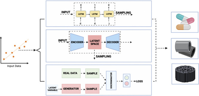
(a) Simple neural network with an input layer, a single hidden layer, and an output layer. The node in the hidden layer has a bias (b1) associated with it, while the mapping from the input layer to the hidden layer has a set of weights (W1, W2, and W3) associated with it. Through the training process, these weights and biases are updated in order to optimize (minimize) the loss function. The function g (often referred to as the activation function) is usually a nonlinear function. (b) A representative illustration of a RNN where the current output depends not only on the current input but also the previous input, making it useful for the generation of sequential data. (c) A representative illustration of a VAE composed of encoder and decoder networks. The encoder converts a discrete data distribution to a continuous latent space, which is converted back to a discrete representation by the decoder. By moving in the latent space, new samples can be generated. (d) A representative illustration of a GAN composed of generator and discriminator networks. Using a probabilistic approach, the generator attempts to create a synthetic data distribution that is very similar to a real distribution, while the discriminator attempts to differentiate between real and synthetic data.

The training process is iterative in nature, with the weights and biases changing with each iteration to minimize the difference between the predicted output and the actual output available from the training data set. The modification to the values of the weights and biases is achieved through a process known as back-propagation.²⁶ The mathematical description of a neural network as described in Figure 2a would appear rather elementary. However, as the number of nodes and hidden layers increases, the problem becomes much more complex and tough to handle. The mathematics of these models are quite complex owing to the sheer number of calculations that need to be performed. As a result, not only are the computational costs associated with them high but also they are highly sensitive to the choice of parameters such as initial weights and biases, learning rates, and choice of loss functions. That being said, if trained correctly, these models are excellent when it comes to the prediction of material properties.

In supervised learning, as discussed earlier, the training data set, S = (x₁,y₁), ..., (x_n,y_n), comprises of a set of inputs along with their desired outputs. In some cases, however, the data set is comprised of just the inputs, S = x₁, ..., x_n. Here, the end goal is not to find a function that can map the inputs to their desired outputs but rather to build a representation of the provided input and use it for tasks such as generating new data or making decisions. Formally known as unsupervised machine-learning algorithms, they come into use when the data are unlabeled, and the main goal is to extract some meaningful information from this unlabeled data set.^44,45 Mathematically, the data x can be considered to be sampled from a probability distribution P(x). The goal of the unsupervised machine-learning algorithm is to “implicitly represent this distribution”,⁴⁵ allowing the generation of artificial data. From a materials research perspective, this could lead to the generation of new molecules or an optimization of the properties of existing ones. Popularly referred to as generative models, in materials research, the most widely used such models are recurrent neural networks (RNNs), variational autoencoders (VAEs), and generative adversarial networks (GANs).

2.1. Recurrent Neural Networks (RNNs)

Recurrent neural networks (RNNs) are a special type of neural networks that are very powerful in the detection of patterns from sequential data and are widely used for sequence modeling and generation. This sequential data could be a time series (for example, the daily COVID-19 cases over the period of 3 months), numerical patterns, or even text. RNNs are the go-to networks for text generation, making them suitable for molecule generation, since the SMILES string is essentially a sequence of characters (text).⁴⁶

The noteworthy feature of the RNN that makes it very desirable for learning sequential data is that it operates in cycles, transmitting information back to itself. In doing so, not only does it account for the current input x_t but also the previous input x_t–1 while computing the output (refer to Figure 2b). Given a long sequence of data x_t–1, .., x₁, the RNN can efficiently estimate P(x_t|x_t–1, ..., x₁). In the scenario that the sequence is very long, it is common practice to restrict the sequence to a short span of length. Another way of looking at this is that the previous information is stored in a hidden variable h_t, which is used to predict an output as = P(x_t – h_t) and in the process gets updated itself, h_t = f(h_t–1, x_t–1). At each step, the weight (W) and bias (b) matrices are computed.^46,47 The training process is completed through the “back-propagation through time” algorithm, where at each time step a loss function is defined, which measures the difference between the computed output and the target output (y_t). Following this, the partial derivatives of this loss function with respect to the weight matrices is computed, based on which the matrices are updated. This cycle continues until the loss function assumes an acceptable value.⁴⁶

There is, however, a flaw in the way a conventional RNN is trained. The partial derivative of the loss function with respect to the weight matrices involves a lot of matrix multiplication. In the case of long sequences, they become susceptible to compounding. In cases where the multiplication is with quantities >1, eventually the gradient becomes very large (“exploding gradient”), while in cases where the multiplication is with quantities <1, eventually the gradient becomes very small (“vanishing gradient”), both of which severely hamper the training process.^46,48 This problem can be overcome using special units known as the “long–short-term memory” (LSTM) units, a detailed description of which can be found in a paper from Hochreiter and Schmidhuber.⁴⁹ Essentially, through the internal states of special units, the architecture is able to ensure a constant error flow, that is neither vanishing nor exploding. Most RNN-based drug/molecule generation algorithms make use of LSTM units.

2.2. Variational Autoencoders (VAEs)

In many cases, it is of great interest, given some real data X, distributed according to an unknown probability distribution P(X), to develop a model P_θ(x), which is very similar to P(X), which can be sampled from to generate new data. Historically, this problem had a few challenges, like models depending on the structure of data, requiring serious approximations, and relying on some very computationally expensive techniques. Newer classes of generative models are able to deal with a majority of these challenges. One such very popular class of models is the Variational Autoencoder (VAE).⁵⁰

Models that learn probability distributions are known as probabilistic models. These models always have some uncertainty associated with them due to the presence of unknowns. In most cases, instead of learning an unconditional model P_θ(x), there is a great interest in learning a conditional model P_θ(y – x) based on a distribution of variables y, conditioned to an observed variable x.⁵¹ This is the case in high-dimensional inputs and outputs like textual data (SMILES string). These models involve latent variables, commonly denoted by z, which are variables, although a part of the model that is not observable and as a result not a part of the data set.⁵¹ Given a probability distribution of the latent variable, P(z), defined over a high-dimensional space , we would like to sample a vector of latent variable z. To do so, a deterministic function f(z; θ) is made use of, which is parametrized by a vector θ, which is fixed, making f(z; θ) a random variable. The goal of the learning process is to optimize θ in such a way that the sampled vector z from the probability distribution P(z) closely resembles the data X in the initially provided data set. Mathematically, the following needs to be maximized⁵⁰

The VAE tries to maximize P_θ(x) as shown above. The VAE gets its name from the (largely unrelated) autoencoder due to similarities in the architecture. A detailed mathematical description of the VAE has been given by Kingma and Welling^51,52 and Doersch.⁵⁰ The VAE consists of two neural networks, an encoder which gives a posterior distribution q_θ(z|x), parametrized by network weights θ, and a decoder, which gives a likelihood distribution p_ϕ(x|z) parametrized by network weights ϕ (refer to Figure 2c). Here the VAE is tasked with measuring how similar these two distributions q_θ(z|x) and p_ϕ(x|z) are. This is most commonly done through the Kullback–Leibler (KL) divergence, denoted by D_KL(q(x)∥p(x)). The KL divergence is non-negative and nonsymmetric (i.e., D_KL(q(x)∥p(x)) ≠ D_KL(p(x)∥q(x))).⁵³ The KL divergence is given by

After rigorous mathematical manipulations, the loss function of the VAE comes to be

This is often known as the “evidence lower bound” (ELBO). Given the loss function, sampling is difficult owing to the complexity of gradient computation. To deal with this, a reparameterization trick is employed where the latent variable (z) is defined as a deterministic variable z = g_ϕ(ϵ, x), where ϵ is an auxiliary variable, which can be sampled from.⁵² This allows an easier gradient computation.

2.3. Generative Adversarial Networks (GANs)

One of the most interesting developments in machine learning over the past 10 years or so is the advent of the generative adversarial network (GAN). Developed by Goodfellow et al.,¹¹⁰ the GAN, as the name suggests, is a generative model made to compete against an adversarial model. The adversarial model, often referred to as a discriminative model, is essentially a classifier that can determine whether a sample of data belongs to the real data distribution or the generated data distribution (refer to Figure 2d).⁵⁴ The working of a GAN can be thought of as being analogous to a game between a counterfeiter and a cop. A generator (in this case the counterfeiter) generates fake currency, while the discriminator (the cop) can differentiate between real and fake currency. While initially it is very easy for a discriminator to differentiate between real and fake currency, with each cycle, the generator updates itself and starts producing more realistic currency. Eventually, a stage is reached where the generated currency is so realistic, that the discriminator’s decision is reduced to a random guess. This marks the end of the training process of the network. Similar to the VAE, the GAN is also a probabilistic model and deals with latent variables z.^54,55 GANs have been shown to produce the best samples as compared to other generative models and have been successfully applied to many tasks such as generating high-quality human faces⁵⁶ and converting aerial images to maps and black-and-white images to colored images.⁵⁷

Given a data set of points χ ∈ IRⁿ, it can be said that the points belong to a probability distribution p(x). The goal is to generate points that are very similar to those in the data set. This raises an important question of how to define similarity? One way of looking at it is to minimize the distance between two points in order to maximize the similarity. This definition is, however, not useful in the present scenario because it is required that irrespective of the distance the points should belong to the same class as the initially provided data set. The best measure of similarity in this case is that between probability distributions. Essentially, a probability distribution (q(x)) needs to be found that closely resembles p(x). This problem is not as simple as it looks. This is because p(x) is unknown. In order to approximate p(x), the GAN starts with some initial distribution r(x), defined on IR^m. In doing so, it attempts to find an ideal mapping G:IR^m → IRⁿ, such that if some random variable z ∈ IR^m comes from a probability distribution r(x) then G(z) comes from a distribution p(x). In order to optimize this mapping, G(z) needs to update its parameters. To aid with this, the discriminator function D(x) (D(x) ∈ [0,1]) can classify the output of G(z) as either real or fake or, in other words, distinguish between the real data p(x) and the generated data G(z), forcing G to update its parameters. This can mathematically be described by the minimax function as follows⁵⁸

In a perfectly trained GAN, D(x) is always equal to 0.5, or in other words, the discriminator can no longer distinguish between the real and the generated samples.

3. Applications of Generative Models in Materials Science

While an understanding of the underlying principles of these models is usually enough to venture into a broad domain of problems, there are some complexities that are unique to materials science that need to be tackled before effectively applying these models. Two major complexities are the availability of data and molecular representation. When it comes to generative models, especially in emerging domains such as materials research, one of the biggest hurdles is the handling and curation of raw structural data. In fact, of the time spent on the development of the generative models, a significant amount is spent on the acquisition, analysis, preprocessing, and featurization of data.^59,60 When it comes to materials research, while certain domains such as organic drug-like molecules have large data sets associated with them, most domains such as energy materials and/or structural materials have little data, making training of data-intensive generative models a rather difficult task. Even the data that are available might be erroneous, containing missing or duplicate entries. The handling and curation of raw structural data is a central component in the workflow of a machine-learning algorithm (refer to Figure 3), making challenges pertaining to them a central bottleneck in the success of generative modeling. Thus, it is essential to have a well-defined protocol for the procurement and use of data.

Figure 3.

Schematic of a workflow for developing a machine-learning model from a materials research perspective. Beginning with the identification of the objective function, the handling and curation of data and molecular featurization have established themselves to be two of the biggest challenges in the success of these models. Each step is critical for the model to work smoothly.

While Table 1 provides a set of publicly available data sets that can be leveraged for machine-learning algorithms, the issue of molecular representation is far more complex and outside the scope of this review. The challenge here essentially is to find a way to represent molecules that is both readable to the computer and understandable to the scientist or the engineer.⁶¹ This representation should be such that it should contain the essential structural features of the molecule under investigation and should ideally be both unique (each molecule has a single representation) and invertible (each representation corresponds to a single molecule).⁶² Finding an effective molecular representation is paramount to the success of a machine-learning model, with the existence of a strong correlation between the accuracy of the prediction and the choice of representation used.⁶³ The commonly used molecular representations include molecular graphs,⁶² the SMILES string,⁶⁴ the InChI string,⁶⁵ and molecular descriptors.⁶⁶ Among these representations, for the purposes of generative modeling, the most important representation is the SMILES string. The SMILES string is essentially a form of notation based on the molecular graph theory, which makes use of natural grammatical rules in order to store and process chemical information. Chemical structures are represented in the form of a linear string of characters, very similar to natural language. The SMILES string has a set of rules (very similar to grammar) for representing atoms, bonds, branches, cyclic structures, disconnected structures, and aromaticity.⁶⁴

Table 1. Nonexhaustive Set of Publicly Available Datasets That Can Be Used for a Wide-Range of Machine-Learning Algorithms in Materials Science.

data set	features	references
PubChem	Information about 109,907,032 unique chemical structures, 271,129,167 chemical entities, and 1,366,265 bioassays	(69)
ZINC	Over 230,000,000 commercially available compounds for the purpose of virtual screening in drug discovery	(70)
CheMBL	Over 2,086,898 bioactive molecules and 17,726,334 bioactivities for effective drug discovery	(71)
ChemDB	Over 5,000,000 commercially available small molecules intended for drug discovery	(72)
ChemSpider	Chemical structure data for over 100,000,000 structures from 276 data soures	(73)
DrugBank	Over 200 data fields each for 14,853 small drugs (including 2687 approved small drugs)	(74)
The Materials Project	Information about 131,613 inorganic compounds, 49,705 molecules, 530,243 nanoporous materials, and 76,194 band structures	(75)
GDB9	17 properties each of 134,000 neutral molecules with up to nine atoms (CONF), with the exception of hydrogen	(76)
Pauling File	Information about 310,000 crystal structures for 140,000 different phases, 44,000 phase diagrams, and 120,000 physical properties	(77)
AFLOW	Information about 3,513,989 material compounds with over 695,769,822 computed properties	(78)
HTEM DB	37,093 compositional, 47,213 structural, 26,577 optical, and 12,849 electrical properties of thin films	(79)
OQMD	DFT-calculated structural and thermodynamic properties of 815,654 materials	(80), (81)
SuperCon	Superconducting properties of 33,284 oxide and metallic samples and 564 organic samples from the literature	(82)

In this section, by exploiting the mathematical principles discussed in the previous section and by using an appropriate molecular representation and data set, we will review the applications of generative models in the domains of biomaterials and organic drug-like molecules, energy materials, and structural materials. Owing to the diverse range of materials to which these models are being applied, there are certain key differences that warrant the adoption of different approaches. The primary difference is that while biomaterials and organic drug-like molecules involve dealing with atomic environments, energy and structural materials involve solid-state crystal environments. Fundamentally, solid-state crystal materials are composed of periodic arrays of repeating units, leading to symmetries at both a local and global level. This symmetry makes it necessary to accommodate periodic boundary conditions because of which conventional models that are used for these materials cannot directly be applied to molecules or atomic environments.⁶⁷ From a machine-learning perspective, the difference between these materials lies in the relevant information they present that needs to be extracted through a process known as “feature extraction” or “feature engineering”. These features are then fed into machine-learning models to make inferences and/or predictions. Feature engineering, especially in the case of solid-state crystalline materials, is rather complex, often involving rigorous mathematical transformations such as the expansion of radial distribution functions,²³ and is outside the scope of this review. An emerging technique for the feature engineering of solid-state crystalline materials is through the use of graph-based networks. Here, crystals are represented graphically through their unit cells, where the atoms that make up the unit cell act as nodes and the distances between these atoms (nodes) serve as edges of the cell.⁶⁷ Newer techniques account for periodic boundary conditions, as is the case with SchNet, a deep-learning architecture based on deep tensor neural networks that model complex atomic interactions while incorporating periodic boundary conditions, in order to predict the formation energies of bulk crytals.⁶⁸ Detailed discussions on feature engineering and advanced techniques to carry it out, especially for solid-state crystalline materials, have been provided by Schmidt et al.²³ and Gong et al.⁶⁷

3.1. Biomaterials and Organic Drug-like Molecules

At the intersection of biological systems and materials science lies the highly interdisciplinary field of biomaterials. Initially intended as materials used in medical devices for safe interaction with biological entities, the scope of these materials has since expanded into biotherapy-related applications such as tissue engineering, drug delivery, and immunomodulation.^83,84 The realm of biomaterials is vast, ranging from the use of metallic materials, to ceramic materials, to polymeric materials and composites, which adds to the challenge of finding the most optimum material or set of materials for the task at hand. With the advent of machine-learning approaches, the field of biomaterials stands to benefit, owing to the ability of machine-learning models to screen large databases, predict material properties, and more importantly generate novel materials. This section intends to focus on the generation of novel polymeric drug-like chemical structures.

3.1.1. RNN-Based Models

As discussed earlier, RNNs are ideal for language models, where, given a sequence of i words or characters (c₁, ..., c_i), they can predict the i + 1^th word or character (c_i + 1). As demonstrated by Segler et al.,⁸⁵ for molecule generation, this sequence of words or characters can be replaced by characters in the SMILES alphabet. They used a data set of 1.4 million SMILES strings from the chEMBL database, with each string being canonicalized. Each SMILES string was encoded using the one-pot representation and used as input to a model consisting of three stacked layers of LSTMs, trained through the back-propagation through time (BPTT) algorithm using the ADAM optimizer.^85,86 The algorithm is able to develop a probability distribution P_θ(s_t+1|s_t, ..., s₁) of the next character in the SMILES string, given the first t characters. This probability distribution can then be sampled to generate novel SMILES strings (molecules).⁸⁵ Bjerrum and Threlfall⁸⁷ used a data set of SMILES strings from the ZINC12 database as input to a neural network consisting of two layers of LSTM units, two hidden layers with a ReLU activation, and an output layer with a softmax activation.⁸⁸ Following this, a sampling model, which had the same architecture as previously described (with minor modifications), was built, which gave an output probability of the next character, which was selected using a multinomial sampler. In doing so they were able to generate two libraries of 50,000 molecules each.⁸⁷ Gupta et al.⁸⁹ used an LSTM-based architecture (refer to Figure 4a), which was fine tuned using transfer learning to generate libraries of SMILES strings that are similar to drugs structurally. Their model was able to perform fragment-based drug discovery, where SMILES strings can be generated starting from a fragment provided by the user. The model essentially grows the fragment provided, by predicting the characters that follow.⁸⁹ Merk et al.⁹⁰ developed a generic model that was able to learn the constitution of molecules (in the SMILES format) from the ChEMBL database. This database was then fine tuned through transfer learning for the “de-novo generation of target specific ligands”.⁹⁰

Figure 4.

(a) Representative illustration of a RNN model for the generation of drug-like molecules. Reprinted from ref (89) under the Creative Commons license (CC BY-NC-ND 4.0). (b) Representative of a VAE model for the generation of drug-like molecules. Reprinted from ref (29) under the Standard ACS AuthorChoice/Editors’ Choice Usage Agreement.

It is difficult to directly optimize molecular characteristics owing to the fact that they are nondifferentiable (back-propagation through time requires the computation of partial derivatives). A way to deal with this is to use a reinforcement learning (RL) framework, which allows chemical space exploration and molecular characteristics optimization without needing to compute loss gradients. Here, a SMILES string is represented as a sequence y = (a₁, ..., a_m), a ∈ D (D is the symbol dictionary). Each symbol in the string corresponds to an action, and the goal of the algorithm is to find a policy to maximize a reward by calculating an action. The only difference in the case of molecule generation is that the reward should only be produced on the completion of the SMILES string generation due to the episodic nature of a molecule.⁹¹ The policy gradient is often performed using the REINFORCE algorithm.⁹² Olivecrona et al.⁹³ introduced a reinforcement learning method to tune RNNs to generate molecules with desirable properties. They found that this method outperforms both standard RNNs and RL methods.

3.1.2. VAE-Based Models

The VAE approach can be used for the de novo generation of molecules, as demonstrated by Gomez-Bombarelli et al.,²⁹ where an encoder was used to convert molecules (discrete data representation) into a continuous vector in the latent space, following which a decoder was used to convert this continuous vector back into a discrete representation (refer to Figure 4b). The advantage of a continuous representation is that performing simple operations within the latent space allows the generation of novel molecules.²⁹ The models were trained on 108 000 molecules from the QM9 database and 250 000 drug-like molecules from the ZINC database. The encoder was a convolutional neural network (CNN),^94,95 and the decoder was a recurrent neural network (RNN), consisting of gated-recurrent units (GRUs).⁹⁶ Gradient-based optimization within the latent space allowed the prediction of the properties of the drug-like molecules generated such as “Quantitative Estimation of Drug-Likeliness” (QED) and “Synthetic Accessibility Score” (SAS). This joint molecule generation and property prediction was carried out by mapping distributions of molecules in the latent space to their corresponding properties through two-dimensional principal component analysis (refer to Figure 5a). This revealed that molecules with high values for a certain property were localized to one particular region, while those with low values were localized to another region.²⁹ Lim et al.⁹⁷ were able to generate drug-like molecules through a conditional variational autoencoder (CVAE) that simultaneously satisfied five target molecular properties. The CVAE is a modified VAE, where the components of the model are conditioned on some observable. In other words, the encoding and decoding are done under some imposed conditions.^97,98 In doing so, the loss function of the VAE is modified depending on the condition c

While Gomez-Bombarelli et al. used a separate neural network for molecular property prediction, Lim et al. incorporated molecular property prediction in the encoder–decoder network. Joo et al.⁹⁹ were able to employ a CVAE to generate valid MAACS fingerprints that were able to satisfy anticancer properties.

Figure 5.

(a) Two-dimensional PCA analysis plots of the variational autoencoder latent space, where the two axes represent the selected properties. The legend on the right of each plot indicates the value of that selected property. The plots in the leftmost column are for the VAE, the central column for the joint VAE-property prediction, and the rightmost column a sample of the latent space. As discussed in Section 3.1.2, in the case of the joint VAE-property prediction, depending on the value of the property, the molecules tend to segregate into localized regions. Reprinted from ref (29) under the Standard ACS AuthorChoice/Editors’ Choice Usage Agreement. (b) The top row represents the starting molecules, while the bottom row represents the generated molecules, along with their similarity index. Reprinted from ref (108) under the Creative Commons Creative Commons Attribution 4.0 International License.

The models discussed thus far make use of the SMILES string representation. While very easy to handle and store, they are very brittle. Small changes in the string can lead to the generation of invalid molecules. VAEs are notorious when it comes to mapping points in the latent space to invalid molecules. A work-around to this was proposed by Kusner et al.,¹⁰⁰ through the grammar variational autoencoder (GVAE), where a context-free grammar was made use of for representing molecules (discrete data). Instead of encoding from and decoding to the SMILES string, parse-trees were made use of, which ensured that the molecules generated were valid.¹⁰⁰ Outside of the inherent brittleness, linear representations like SMILES strings have some other drawbacks. They are not efficient in capturing the similarity between molecules and are not designed to express chemical properties. Jin et al.¹⁰¹ hypothesized that these shortcomings can be dealt with by using molecular graphs. They went on to propose the junction-tree variational autoencoder (JT-VAE) that is able to generate molecular graphs. Instead of generating the molecule atom-by-atom, the model generates a tree-structure consisting of chemically valid subgraphs. Following this, these subgraphs are brought together to generate a molecular graph. They found that the JT-VAE outperforms other models when it comes to molecule generation and optimization.¹⁰¹ Ward et al.¹⁰² were able to make use of the JT-VAE to generate molecules with high similarity to drugs intended for the treatment of severe acute respiratory syndrome (SARS).

3.1.3. GAN-Based Models

Conventional GANs cannot be applied to discrete data (such as SMILES strings and other molecular representations) owing to their nondifferentiability, which makes it challenging to compute gradients and perform back-propagation for optimization. Yu et al.¹⁰³ proposed a workaround to this challenge through a sequence generation framework, SeqGAN. They were able to do so by treating the generator as an agent in a reinforcement learning environment. From a text generation perspective, the characters generated up to a time step are treated as the state, and the next character to be generated is treated as the action. The discriminator evaluates the sequence of characters generated and relays feedback to the generator. The generator is trained by updating the policy gradient.¹⁰³ Another workaround was proposed by Che et al.,¹⁰⁴ through the maximum likelihood augmented discrete generative adversarial network (MaliGAN). Instead of directly focusing on optimizing the GAN, they developed a novel objective by making use of the discriminator’s output. The objective they developed corresponds to the log likelihood and makes use of techniques like importance sampling and variance reduction. This objective becomes much easier to optimize than the conventional one, allowing convenient modeling of discrete data.¹⁰⁴

Guimaraes et al.¹⁰⁵ were able to build upon the SeqGAN, through the objective-reinforced generative adversarial network (ORGAN), and use it for molecule generation. The reward function is a linear combination of the disciminator output and a domain-specific objective (for example, a task like molecule generation will have a different objective than music generation). In addition, mechanisms to ensure that nonunique generated sequences are penalized were put in place. The generator had an RNN-based architecture and the discriminator a CNN-based architecture. The model was trained on 5000 drug-like and non-drug-like molecules from the ZINC database, and the objectives were chosen keeping in mind drug discovery, like solubility, synthesizability, and drug-likeliness.¹⁰⁵ Cao and Kipf¹⁰⁶ were able to develop MolGAN, which can directly generate molecular graphs. Instead of dealing with the SMILES string, the MolGAN operates on molecular-graph-based representations and in doing so generates nearly 100% valid molecules. The objective is reinforcement learning based (the same as ORGAN) and is tuned to generate molecules with desired chemical properties. The model architecture consists of a generator, discriminator, and reward network (mimics the reward function) and is trained on the QM9 data set.¹⁰⁶ Tsujimoto et al.¹⁰⁷ recently developed the L-MolGAN which is optimized to generate larger molecular graphs as compared to the MolGAN. While the frameworks discussed above are very good at generating molecules, many of them end up generating molecules that are very difficult to synthesize. In order to address this, Maziarka et al.¹⁰⁸ developed the Mol-CycleGAN, based on the CycleGAN¹⁰⁹ framework, which generates structurally similar molecules based on an initially provided molecule. In doing so, it helps in generating not only more easily synthesizable molecules but also more optimized molecules with desired properties owing to structural similarities.¹⁰⁸ By using a molecule as a starting point, they were able to generate novel molecules that had a high similarity to this starting molecule, where these similarities were measured using a metric known as the “Tanimoto” similarity. Interestingly, these generated molecules were seen to be neither a random sampling of the latent space nor a memorization of it (refer to Figure 5b).

Owing to the COVID19 pandemic, there was a strong sense of urgency to either find or develop drugs to effectively combat the disease. While a lot of time and resources were diverted toward high-throughput screening to search for existing drugs that could potentially treat the disease, a section of researchers began developing generative models for the de novo design of drugs for the same. Zhavoronkov and colleagues¹¹⁰ developed a novel “generative chemistry pipeline” which made use of crystal structure data for designing novel drug-like molecules to combat COVID19. Their pipeline employed generative models like GANs and generative autoencoders.^110,111

3.2. Energy Materials

Due to an exponential rise in the consumption of energy and a steep increase in the concentration of CO₂ in the atmosphere, there is a lot of research focused on accelerated energy materials discovery. Here, machine learning can be used for the interpretation and design of experiments, faster high-throughput screening, and the output of optimized materials on the input of desired properties.¹¹² This section aims to shed light on the advances in energy materials through generative modeling in photovoltaics (PVs), batteries, and superconductors.

3.2.1. Photovoltaic Materials

Solar energy is converted to electricity using special materials known as semiconducting photovoltaics (PVs). Whether a material can be classified as a PV or not depends on its long-term stability and solar conversion efficiency (SCE). These PVs could be organic or perovskites.^113,114 Conventional machine-learning models have been widely used to study PVs and predict their SCEs. For example, Sun et al.¹¹⁵ were able to use a convolutional neural network (CNN) based deep-learning architecture to predict the solar conversion efficiency (SCE) of OPV materials with 91% accuracy. Interestingly, attempts have been made to generate novel materials with desirable optoelectronic properties to serve as potential PVs. Recently, Jelfs and co-workers¹¹⁶ developed an RNN-based deep generative model (refer to Figure 6a) to produce novel donor–acceptor oligomers as potential candidates for organic PVs. Owing to the existing data on donor–acceptor oligomers not being sufficient for training a robust RNN-based model, they employed transfer learning techniques. By doing so, they explored the chemical space of donor–acceptor oligomers having an optical gap (HOMO–LUMO) ≤ 2 eV and a dipole moment <2 D. Their methodology generated over 1700 oligomers having these properties, making them promising candidates for organic PVs. Two noteworthy points in this study are that, following adequate training, over 90% of the generated molecules were valid, and each of the shortlisted “promising” candidates were fairly synthetically viable. That being said, out of 90 randomly selected generated molecules, only 22 had ideal dipole moments, which indicates a higher variance for predicting the dipole moments.¹¹⁶ When it comes to perovskites, Gao et al.¹¹⁷ used GANs to discover structure–property relationships. Their framework, called MATGANIP, employed a combination of GANs, CNNs, LSTMs, and graph networks to build quantitative material structure–property (QMSP) relationships in these materials using a DFT-generated data set. Here the CNN and graph network is used to extract meaningful structural information to be fed into the generater, while the LSTM is used to improve the identification of the distribution that is fed into the discriminator. Quite impressively, their models were able to achieve mean absolute error rates of 0.01% for the development of these structure–property relationships.¹¹⁷ Quite recently, Hu and colleagues developed CubicGAN, a GAN-based deep neural network model for the inverse design of cubic materials, with applications pertaining to photovoltaics. Trained on a database of upward of 375 000 ternary materials, their model generated over 10 million ternary and 10 million quaternary structures for high-throughput screening. After filtering down the materials, they went on to carry out DFT optimization of materials to determine their stability. In doing so, they were able to identify close to 506 new stable materials for a wide range of applications including photovoltaics.¹¹⁸

Figure 6.

(a) Representative illustration of a workflow for the generation of potential donor–acceptor oligomers to serve as photovoltaic materials. Here the specialized RNN was finely tuned for the generation of the said oligomers. Reprinted from ref (116) under the Creative Commons license (CC BY-NC 3.0). (b) A representative of the architecture of the conditional GAN used to produce realistic data samples from existing HEA data sets by generating samples from the latent space. Reprinted from ref (128) under the Creative Commons license (CC BY-NC-ND 4.0).

3.2.2. Battery Materials

Outside of solar energy, another important avenue that can help transition toward the adoption of cleaner energy practices is rechargeable batteries. While some advanced materials do exist here, such as lithium batteries, they are plagued with problems such as dendrite formation on plating. These inherent challenges make it difficult to further improve the properties of the existing materials, motivating a search for better materials using machine-learning techniques.^112,119 To this end, researchers have had some success using conventional machine-learning algorithms. For example, Joshi et al.¹²⁰ used SVMs and neural networks to predict the electrode voltage of metal-ion batteries using a data set of 3977 instances of DFT-computed voltages of Li, Mg, Ca, Zn, Al, and Y based metal-ion batteries. While this approach does have its merits, the structure to property prediction route largely limits the exploration of the chemical space, making the task of finding an optimum material more complex. An alternate to this is inverse design, where novel chemical structures are generated based on certain target properties. Bhowmick et al.¹²¹ suggest that deep generative models would be effective for the representation and modeling of interphases of battery materials. The main challenge when it comes to battery materials is that the interphase is not static, and it undergoes changes during its lifetime depending on the battery composition. The inherent uncertainty that underlies this process can be captured using RNNs owing to their ability to effectively predict P(x_t|x_t–1, ..., x₁) given data instances x_t–1, ..., x₁ (refer to Section 2.1). Bhowmick and colleagues suggest employing gradient descent based algorithms to search for optimum configurations that satisfy the desired material performance metrics. One issue in this case, as is the major issue with most material science based problems, is finding an optimum representation. It has been suggested that either VAEs or GANs be used for representing and classifying battery interphases owing to the development of a continuous latent representation and the ability to work with smaller incomplete data sets. Despite the promise of these models, a closed-loop interphase design for batteries making use of physical models, experiments, and data-derived approaches is a long way out.¹²¹ Hu and co-workers were able to generate over 2 million samples with a novelty of over 92% of inorganic materials using a GAN-based architecture MatGAN. Their analysis showed that their model was able to achieve a much higher efficiency when it came to the sampling of the inorganic chemical space compared to other techniques, achieving an 84.5% chemical validity. They claim that their model can be extended for the generation of electrolyte- and battery-like materials.¹²²

3.2.3. Superconducting Materials

Superconductors are materials that conduct electric current with zero resistance. This phenomenon is usually observed below a critical temperature (T_C), which is a property of the material. The first superconductor, mercury (Hg), was discovered in the year 1911 and had a critical temperature of 4.2 K. In order to attain and maintain such low temperatures, expensive techniques like helium cooling are required, which is not viable if this phenomenon is to be exploited on a larger scale. Applications like these require superconducting materials with much higher T_C, close to room temperature. For a long time, it was believed that high-temperature superconductors were impossible to achieve, with a limit of 25 K on the T_C. This hypothesis was however disproved by the discovery of near room-temperature superconductors, with a T_C of 250 K at high pressures.¹²³ The highest T_C achieved at atmospheric pressure was above 130 K.^124,125 The general route to the discovery of superconductors relies on empirical knowledge, intuition, and laborious experimental trial and error. Researchers use an existing superconducting material as their starting point and perform modifications on them. This is not only time-consuming but also restricts the exploration of the chemical space.¹²⁶ This motivates the use of machine learning in the screening and discovery of possible high T_C superconducting materials.

Recently, Kim et al.¹²⁷ adopted a variational bayesian neural network approach to predict the critical temperature of potentially superconducting materials. Broken down into two stages, their model first finds a mutual correlation between superconducting materials and their T_C and then, through Monte Carlo sampling, determines and evaluates the predictive performance of the material. One advantage of this approach over conventional models such as RFs and SVMs is that this approach is not prone to overfitting due to the presence of the sampling algorithm in the second stage which provides a probability of correlation of parameters of the material to the T_C, instead of fitting them with a standard linear regression. While the mathematics of this model will not be discussed in this paper, the underlying mathematical principles are very similar to those developed for the VAE (refer to Section 2.2). The performance of this model was almost at par with the best performing model for the same task, with this model outperforming its competition in certain performance metrics.¹²⁷

3.3. Structural Materials

Materials are chosen for particular applications depending upon their properties; for example, materials with ideal electronic properties are often used as electronic materials and those with ideal optical properties as optical materials. Similarly, if a material has ideal mechanical properties, it is employed as a structural material. Structural materials, as the name suggests, are used for load bearing in structures. The route to structural materials discovery is painstakingly long, involving “materials selection, process engineering, product design, structure–property optimization, multiscale modeling, process optimization and failure analysis, safety precautions, real-life trials, and pilot-scale operations”.¹²⁹ This presents the perfect opportunity to use machine-learning techniques to speed up the structural materials discovery process.^129,130 Researchers have had some success in structural material property prediction using conventional machine-learning algorithms. For example, Lee et al.¹³¹ were able to predict both the ultimate tensile strength and yield strength of over 5000 thermomechanically controlled processed steel alloys using 16 chemical descriptors. They employed 16 machine-learning algorithms including linear regression, RFs, SVMs, and gradient-boosted trees. They observed that the nonlinear algorithms outperformed the linear algorithms, with many of the algorithms producing acceptable results.¹³¹

As opposed to organic drug-like materials and even energy materials, structural materials have not been explored much using generative models with the exception of high-entropy alloys (HEAs). HEAs are engineered materials with five or more principal component elements, each with an atomic percent of 5–35 at %.¹³² HEAs are of special interest owing to their unique crystalline random solid solution (RSS) structures, in which each of the five or more constituent elements can occupy a lattice site with equal probability. Due to this, HEAs possess excellent physical, chemical, and mechanical properties.^130,132 The extraordinary properties of HEAs arise out of four effects closely linked to the RSS. The first is the high-entropy effect, described by the configurational entropy, ΔS_mix, given by

where R is the universal gas constant and X_i is the concentration of the i^th constituent. Owing to a high number of constituents, the entropy is high, as a result of which the Gibbs free energy of mixing, ΔG_mix, is low enough, allowing a stable formation of the HEA (ΔG_mix = ΔH_mixTΔS_mix). The second effect is the lattice distortion arising due to strain that develops as a result of atomic size misfit. The next is the slow diffusion kinetics, which leads to high structural stability. The last effect is the “cocktail effect”, where constituents are selected with specific properties in mind.¹³² The chemical space for the exploration of potential HEAs is vast, and using conventional techniques is both time-consuming and expensive, making generative modeling a promising alternative. Lee et al.¹²⁸ developed a deep-learning method for the phase prediction of HEAs. While the model for predicting phases was a deep neural network, a conditional GAN (refer to Figure 6b) was used to produce realistic data samples from existing HEA data sets by generating samples from the latent space. The only difference here from a conventional GAN is that the model was conditioned to compensate for different proportions of phase data in the initial data set. From 989 normalized samples in the initial data, their GAN model was able to generate 200 samples for each phase, completely different from the original data. This augmented data set helped achieve a 93.17% testing accuracy for all phases.¹²⁸ Debnath and colleagues¹³³ also employed conditional GANs, but for inverse design of HEAs as opposed to phase prediction. The main advantage of conditional GANs for inverse design is that owing to additional conditioning vectors put in place they offer greater control over the output as opposed to conventional GANs, which require many samples to be drawn from real data before candidates can be generated. One disadvantage observed here was that conditional GANs are difficult to work with owing to a high degree of hyperparameter tuning but, in return, provide superior results as compared to alternate models such as VAEs. By identifying desirable shear modulus and fracture toughness, the conditioning vector helped bias the generator toward likely compositions that exhibit the required properties. Depending on the required properties, the GAN architecture was able to choose elements that could approach these properties.¹³³

4. Conclusions and Future Outlook

We presented the need for the application of machine-learning techniques, in particular generative models in materials discovery, design, and optimization, and the underlying theory and mathematical principles behind the working of these generative models and discussed state-of-the-art applications of these models in the domains of biomaterials and organic drug-like materials, energy materials, and structural materials. Generative models differ from other conventional computational approaches such as genetic algorithms in terms of their mathematical rigor and the underlying principles through which they operate. Generative models rely less on rules set by researchers or scientists and tend to learn to perform tasks instead of simply performing certain tasks, as opposed to techniques such as genetic algorithms that follow selective operations facilitating the evolution of a population of candidate solutions.¹³⁴ Conventional techniques rely heavily on using predefined (often rigorous) mathematical approaches, while generative models use data-intensive approaches. Evidently, while the use of generative models is beneficial in scenarios where data are abundant, these models tend to fail dramatically in evolving domains, plagued by data scarcity. Keeping these limitations in mind, researchers have cleverly begun using these methods as a supplement to more conventional techniques such as MD¹³⁵ and genetic algorithms.¹³⁴

Despite the promise of these techniques, there are several challenges that lie ahead in their wide-range applications. The biggest challenge that one can foresee is the availability of appropriate data. As discussed in Table 1, most material databases deal with organic drug-like molecules, as a result of which most applications of these models lie in the same domain. On the other hand, data on energy and/or structural materials are harder to come by, making it difficult to train generative models as they are data intensive. A focused effort toward better data collection and curation practices could help tackle this problem.

A second challenge that is exclusive to generative models is the synthetic viability of the generated materials. As discussed in Section 3, while a high percentage of the generative model generated chemical structures are valid, a significant amount of these structures are not synthetically viable. This essentially implies that while the generated structures are theoretically feasible it is difficult to synthesize them experimentally. The reason for this is that a miniscule fraction of the chemical space has been accessed to date,⁸⁹ so when the generative model produces novel materials outside the accessed space the complexity and cost associated with synthetically producing the material are very high. This issue is largely associated with generative models in general because their predictions lie outside the purview of the data provided as input, and this is something most researchers have failed to address. This could be because the training data, which are usually DFT generated, contain a high number of synthetically nonviable structures. Since generative models work on replicating the probability distributions of the provided data, there is a high chance that the generated molecules, although theoretically feasible, are synthetically nonviable. Smarter data collection, curation, and featurization could be a route to improving the synthetic viability of the generated molecules.

Lastly, there is a lack of understanding of the functioning of these generative models, especially complex ones such as VAEs and GANs. Most researchers tend to treat these models as black-boxes, making error analysis a difficult task. A systematic understanding of how these models work and how the parameters that are fed into them affect their performance would aid in a better design of advanced materials for an enhanced performance in intended applications. This dynamic area of research is constantly evolving. A focused approach toward the discovery, design, and optimization of materials would go a long way in the advancement of various domains of materials science such as biomaterials, energy materials, and structural materials.

The authors declare no competing financial interest.

References

- Olson G. B. Designing a New Material World. Science 2000, 288, 993–998. 10.1126/science.288.5468.993. [DOI] [Google Scholar]
- Hong S.; et al. Reducing Time to Discovery: Materials and Molecular Modeling, Imaging, Informatics, and Integration. ACS Nano 2021, 15, 3971–3995. 10.1021/acsnano.1c00211. [DOI] [PubMed] [Google Scholar]
- Correa-Baena J.-P.; Hippalgaonkar K.; van Duren J.; Jaffer S.; Chandrasekhar V. R.; Stevanovic V.; Wadia C.; Guha S.; Buonassisi T. Accelerating Materials Development via Automation, Machine Learning, and High-Performance Computing. Joule 2018, 2, 1410–1420. 10.1016/j.joule.2018.05.009. [DOI] [Google Scholar]
- Liu Y.; Zhao T.; Ju W.; Shi S. Materials discovery and design using machine learning. J. Materiomics 2017, 3, 159–177. 10.1016/j.jmat.2017.08.002. [DOI] [Google Scholar]
- About J.Materials genome initiative for global competitiveness; National Science and Technology Council, USA, 2011. https://www.mgi.gov/sites/default/files/documents/materials_genome_initiative-final.pdf.
- Lipinski C.; Hopkins A. Navigating chemical space for biology and medicine. Nature 2004, 432, 855–861. 10.1038/nature03193. [DOI] [PubMed] [Google Scholar]
- Dobson C. M.; et al. Chemical space and biology. Nature 2004, 432, 824–828. 10.1038/nature03192. [DOI] [PubMed] [Google Scholar]
- Schneider G.; Fechner U. Computer-based de novo design of drug-like molecules. Nat. Rev. Drug Discovery 2005, 4, 649–663. 10.1038/nrd1799. [DOI] [PubMed] [Google Scholar]
- Kutchukian P. S.; Shakhnovich E. I. De novo design: balancing novelty and confined chemical space. Expert Opin. Drug Discovery 2010, 5, 789–812. 10.1517/17460441.2010.497534. [DOI] [PubMed] [Google Scholar]
- Kumar A.; Zhang K. Y. Hierarchical virtual screening approaches in small molecule drug discovery. Methods 2015, 71, 26–37. 10.1016/j.ymeth.2014.07.007. [DOI] [PMC free article] [PubMed] [Google Scholar]
- Schneider G. Trends in virtual combinatorial library design. Curr. Med. Chem. 2002, 9, 2095–2101. 10.2174/0929867023368755. [DOI] [PubMed] [Google Scholar]
- Szymański P.; Markowicz M.; Mikiciuk-Olasik E. Adaptation of high-throughput screening in drug discovery—toxicological screening tests. Int. J. Mol. Sci. 2012, 13, 427–452. 10.3390/ijms13010427. [DOI] [PMC free article] [PubMed] [Google Scholar]
- Tanrikulu Y.; Krüger B.; Proschak E. The holistic integration of virtual screening in drug discovery. Drug Discovery Today 2013, 18, 358–364. 10.1016/j.drudis.2013.01.007. [DOI] [PubMed] [Google Scholar]
- Armstrong J. A review of high-throughput screening approaches for drug discovery. Am. Biotechnol. Lab. 1999, 17, 26–28. [Google Scholar]
- Sliwoski G.; Kothiwale S.; Meiler J.; Lowe E. W. Computational methods in drug discovery. Pharmacol. Rev. 2014, 66, 334–395. 10.1124/pr.112.007336. [DOI] [PMC free article] [PubMed] [Google Scholar]
- Devi R. V.; Sathya S. S.; Coumar M. S. Evolutionary algorithms for de novo drug design–A survey. Applied Soft Computing 2015, 27, 543–552. 10.1016/j.asoc.2014.09.042. [DOI] [Google Scholar]
- Nishibata Y.; Itai A. Automatic creation of drug candidate structures based on receptor structure. Starting point for artificial lead generation. Tetrahedron 1991, 47, 8985–8990. 10.1016/S0040-4020(01)86503-0. [DOI] [Google Scholar]
- Gillet V. J.; Newell W.; Mata P.; Myatt G.; Sike S.; Zsoldos Z.; Johnson A. P. SPROUT: recent developments in the de novo design of molecules. J. Chem. Inf. Model. 1994, 34, 207–217. 10.1021/ci00017a027. [DOI] [PubMed] [Google Scholar]
- Schneider G.; Lee M.-L.; Stahl M.; Schneider P. De novo design of molecular architectures by evolutionary assembly of drug-derived building blocks. J. Comput.-Aided Mol. Des. 2000, 14, 487–494. 10.1023/A:1008184403558. [DOI] [PubMed] [Google Scholar]
- Nicolaou C. A.; Apostolakis J.; Pattichis C. S. De novo drug design using multiobjective evolutionary graphs. J. Chem. Inf. Model. 2009, 49, 295–307. 10.1021/ci800308h. [DOI] [PubMed] [Google Scholar]
- Argaman N.; Makov G. Density functional theory: An introduction. Am. J. Phys. 2000, 68, 69–79. 10.1119/1.19375. [DOI] [Google Scholar]
- Allen M. P. Introduction to molecular dynamics simulation. Computational soft matter: from synthetic polymers to proteins 2004, 23, 1–28. [Google Scholar]
- Schmidt J.; Marques M. R.; Botti S.; Marques M. A. Recent advances and applications of machine learning in solid-state materials science. npj Comput. Mater. 2019, 5, 1–36. 10.1038/s41524-019-0221-0. [DOI] [Google Scholar]
- Beham M. P.; Roomi S. M. M. A review of face recognition methods. International Journal of Pattern Recognition and Artificial Intelligence 2013, 27, 1356005. 10.1142/S0218001413560053. [DOI] [Google Scholar]
- Chen H.; Engkvist O.; Wang Y.; Olivecrona M.; Blaschke T. The rise of deep learning in drug discovery. Drug Discovery Today 2018, 23, 1241–1250. 10.1016/j.drudis.2018.01.039. [DOI] [PubMed] [Google Scholar]
- Vamathevan J.; Clark D.; Czodrowski P.; Dunham I.; Ferran E.; Lee G.; Li B.; Madabhushi A.; Shah P.; Spitzer M.; et al. Applications of machine learning in drug discovery and development. Nat. Rev. Drug Discovery 2019, 18, 463–477. 10.1038/s41573-019-0024-5. [DOI] [PMC free article] [PubMed] [Google Scholar]
- Ruthotto L.; Haber E. An introduction to deep generative modeling. GAMM-Mitteilungen 2021, e202100008. [Google Scholar]
- Turhan C. G.; Bilge H. S.. Recent trends in deep generative models: a review. 2018 3rd International Conference on Computer Science and Engineering; UBMK, 2018; pp 574–579.
- Gómez-Bombarelli R.; Wei J. N.; Duvenaud D.; Hernández-Lobato J. M.; Sánchez-Lengeling B.; Sheberla D.; Aguilera-Iparraguirre J.; Hirzel T. D.; Adams R. P.; Aspuru-Guzik A. Automatic chemical design using a data-driven continuous representation of molecules. ACS Cent. Sci. 2018, 4, 268–276. 10.1021/acscentsci.7b00572. [DOI] [PMC free article] [PubMed] [Google Scholar]
- Wei J.; Chu X.; Sun X.-Y.; Xu K.; Deng H.-X.; Chen J.; Wei Z.; Lei M. Machine learning in materials science. InfoMat 2019, 1, 338–358. 10.1002/inf2.12028. [DOI] [Google Scholar]
- Butler K. T.; Davies D. W.; Cartwright H.; Isayev O.; Walsh A. Machine learning for molecular and materials science. Nature 2018, 559, 547–555. 10.1038/s41586-018-0337-2. [DOI] [PubMed] [Google Scholar]
- Pilania G. Machine learning in materials science: From explainable predictions to autonomous design. Comput. Mater. Sci. 2021, 193, 110360. 10.1016/j.commatsci.2021.110360. [DOI] [Google Scholar]
- Juan Y.; Dai Y.; Yang Y.; Zhang J. Accelerating materials discovery using machine learning. J. Mater. Sci. Technol. 2021, 79, 178–190. 10.1016/j.jmst.2020.12.010. [DOI] [Google Scholar]
- Simeone O. A very brief introduction to machine learning with applications to communication systems. IEEE Transactions on Cognitive Communications and Networking 2018, 4, 648–664. 10.1109/TCCN.2018.2881442. [DOI] [Google Scholar]
- Ayodele T. O. Types of machine learning algorithms. New Advances in Machine Learning 2010, 3, 19–48. [Google Scholar]
- Kotsiantis S. B.; Zaharakis I.; Pintelas P. Supervised machine learning: A review of classification techniques. Emerging artificial intelligence applications in computer engineering 2007, 160, 3–24. [Google Scholar]
- Cunningham P.; Cord M.; Delany S. J.. Machine Learning Techniques for Multimedia; Springer, 2008; pp 21–49. [Google Scholar]
- Wolf M. M.Mathematical foundations of supervised learning. Lecture notes from Technical University of Munich, 2018. [Google Scholar]
- Singh A.; Thakur N.; Sharma A.. A review of supervised machine learning algorithms. 2016 3rd International Conference on Computing for Sustainable Global Development; INDIACom, 2016; pp 1310–1315.
- Kingsford C.; Salzberg S. L. What are decision trees?. Nat. Biotechnol. 2008, 26, 1011–1013. 10.1038/nbt0908-1011. [DOI] [PMC free article] [PubMed] [Google Scholar]
- Noble W. S. What is a support vector machine?. Nat. Biotechnol. 2006, 24, 1565–1567. 10.1038/nbt1206-1565. [DOI] [PubMed] [Google Scholar]
- Shiloh-Perl L.; Giryes R. Introduction to deep learning. arXiv preprint 2020, 10.48550/arXiv:2003.03253. [DOI] [Google Scholar]
- Ghahramani Z.Unsupervised learning; Summer School on Machine Learning, 2003; pp 72–112. [Google Scholar]
- Neupert T.; Fischer M. H.; Greplova E.; Choo K.; Denner M. Introduction to Machine Learning for the Sciences. arXiv 2021, 10.48550/arXiv.2102.04883. [DOI] [Google Scholar]
- Schmidt R. M. Recurrent neural networks (rnns): A gentle introduction and overview. arXiv preprint 2019, 10.48550/arXiv:1912.05911. [DOI] [Google Scholar]
- Zhang A.; Lipton Z. C.; Li M.; Smola A. J.. Dive into Deep Learning. https://d2l.ai (accessed 2020).
- Nicholson C.A beginner’s guide to lstms and recurrent neural networks. Skymind: Saatavissa, Hakupäivä, 2019.https://skymind.ai/wiki/lstm.
- Hochreiter S.; Schmidhuber J. Long short-term memory. Neural Comput 1997, 9, 1735–1780. 10.1162/neco.1997.9.8.1735. [DOI] [PubMed] [Google Scholar]
- Doersch C. Tutorial on variational autoencoders. arXiv preprint 2016, 10.48550/arXiv:1606.05908. [DOI] [Google Scholar]
- Kingma D. P.; Welling M. An introduction to variational autoencoders. arXiv preprint 2019, 10.48550/arXiv:1906.02691. [DOI] [Google Scholar]
- Kingma D. P.; Welling M. Auto-encoding variational bayes. arXiv preprint 2013, 10.48550/arXiv:1312.6114. [DOI] [Google Scholar]
- Odaibo S. Tutorial: Deriving the standard variational autoencoder (vae) loss function. arXiv preprint 2019, 10.48550/arXiv:1907.08956. [DOI] [Google Scholar]
- Goodfellow I.; Pouget-Abadie J.; Mirza M.; Xu B.; Warde-Farley D.; Ozair S.; Courville A.; Bengio Y. Generative adversarial networks. Commun. ACM 2020, 63, 139–144. 10.1145/3422622. [DOI] [Google Scholar]
- Goodfellow I. Nips 2016 tutorial: Generative adversarial networks. arXiv preprint 2016, 10.48550/arXiv:1701.00160. [DOI] [Google Scholar]
- Karras T.; Laine S.; Aila T.. A style-based generator architecture for generative adversarial networks. Proc. IEEE/CVF Conf. Comp. Vis. Pattern Recog. 2019; pp 4401–4410. [DOI] [PubMed]
- Isola P.; Zhu J.-Y.; Zhou T.; Efros A. A.. Image-to-image translation with conditional adversarial networks. Proc. IEEE Conf. Comp. Vis. Pattern Recog. 2017; pp 1125–1134.
- Wang Y. A Mathematical Introduction to Generative Adversarial Nets (GAN). arXiv preprint 2020, 10.48550/arXiv:2009.00169. [DOI] [Google Scholar]
- Roh Y.; Heo G.; Whang S. E. A survey on data collection for machine learning: a big data-ai integration perspective. IEEE Trans. Knowl. Data Eng. 2019, 10.1109/TKDE.2019.2946162. [DOI] [Google Scholar]
- Whang S. E.; Lee J.-G. In Data collection and quality challenges for deep learning, Proceedings of the VLDB Endowment, 2020, 13, ((12)), , pp 3429––3432..
- David L.; Thakkar A.; Mercado R.; Engkvist O. Molecular representations in AI-driven drug discovery: a review and practical guide. J. Cheminf. 2020, 12, 1–22. 10.1186/s13321-020-00460-5. [DOI] [PMC free article] [PubMed] [Google Scholar]
- Elton D. C.; Boukouvalas Z.; Fuge M. D.; Chung P. W. Deep learning for molecular design—a review of the state of the art. Mol. Syst. Des. Eng. 2019, 4, 828–849. 10.1039/C9ME00039A. [DOI] [Google Scholar]
- Chuang K. V.; Gunsalus L. M.; Keiser M. J. Learning molecular representations for medicinal chemistry: miniperspective. J. Med. Chem. 2020, 63, 8705–8722. 10.1021/acs.jmedchem.0c00385. [DOI] [PubMed] [Google Scholar]
- Weininger D. SMILES, a chemical language and information system. 1. Introduction to methodology and encoding rules. J. Chem. Inf. Model. 1988, 28, 31–36. 10.1021/ci00057a005. [DOI] [Google Scholar]
- Heller S. R.; McNaught A.; Pletnev I.; Stein S.; Tchekhovskoi D. InChI, the IUPAC international chemical identifier. J. Cheminf. 2015, 7, 1–34. 10.1186/s13321-015-0068-4. [DOI] [PMC free article] [PubMed] [Google Scholar]
- Cereto-Massagué A.; Ojeda M. J.; Valls C.; Mulero M.; Garcia-Vallvé S.; Pujadas G. Molecular fingerprint similarity search in virtual screening. Methods 2015, 71, 58–63. 10.1016/j.ymeth.2014.08.005. [DOI] [PubMed] [Google Scholar]
- Gong W.; Yan Q. Graph-based deep learning frameworks for molecules and solid-state materials. Comput. Mater. Sci. 2021, 195, 110332. 10.1016/j.commatsci.2021.110332. [DOI] [Google Scholar]
- Schütt K. T.; Sauceda H. E.; Kindermans P.-J.; Tkatchenko A.; Müller K.-R. Schnet–a deep learning architecture for molecules and materials. J. Chem. Phys. 2018, 148, 241722. 10.1063/1.5019779. [DOI] [PubMed] [Google Scholar]
- Kim S.; Chen J.; Cheng T.; Gindulyte A.; He J.; He S.; Li Q.; Shoemaker B. A.; Thiessen P. A.; Yu B.; et al. PubChem in 2021: new data content and improved web interfaces. Nucleic Acids Res. 2021, 49, D1388–D1395. 10.1093/nar/gkaa971. [DOI] [PMC free article] [PubMed] [Google Scholar]
- Sterling T.; Irwin J. J. ZINC 15–ligand discovery for everyone. J. Chem. Inf. Model. 2015, 55, 2324–2337. 10.1021/acs.jcim.5b00559. [DOI] [PMC free article] [PubMed] [Google Scholar]
- Davies M.; Nowotka M.; Papadatos G.; Dedman N.; Gaulton A.; Atkinson F.; Bellis L.; Overington J. P. ChEMBL web services: streamlining access to drug discovery data and utilities. Nucleic Acids Res. 2015, 43, W612–W620. 10.1093/nar/gkv352. [DOI] [PMC free article] [PubMed] [Google Scholar]
- Chen J. H.; Linstead E.; Swamidass S. J.; Wang D.; Baldi P. ChemDB update—full-text search and virtual chemical space. Bioinformatics 2007, 23, 2348–2351. 10.1093/bioinformatics/btm341. [DOI] [PubMed] [Google Scholar]
- Pence H. E.; Williams A.. ChemSpider: an online chemical information resource. In Journal of Chemical Education; ACS Publications, 2010, 87, (11), , pp 1123––1124.. [Google Scholar]
- Wishart D. S.; Feunang Y. D.; Guo A. C.; Lo E. J.; Marcu A.; Grant J. R.; Sajed T.; Johnson D.; Li C.; Sayeeda Z.; et al. DrugBank 5.0: a major update to the DrugBank database for 2018. Nucleic Acids Res. 2018, 46, D1074–D1082. 10.1093/nar/gkx1037. [DOI] [PMC free article] [PubMed] [Google Scholar]
- Jain A.; Ong S. P.; Hautier G.; Chen W.; Richards W. D.; Dacek S.; Cholia S.; Gunter D.; Skinner D.; Ceder G.; et al. Commentary: The Materials Project: A materials genome approach to accelerating materials innovation. APL Mater. 2013, 1, 011002. 10.1063/1.4812323. [DOI] [Google Scholar]
- Ramakrishnan R.; Dral P. O.; Rupp M.; Von Lilienfeld O. A. Quantum chemistry structures and properties of 134 kilo molecules. Sci. Data 2014, 1, 1–7. 10.1038/sdata.2014.22. [DOI] [PMC free article] [PubMed] [Google Scholar]
- Villars P.; Cenzual K.; Gladyshevskii R.; Iwata S. Pauling File: Toward a Holistic View. Mater. Inf.: Methods, Tools and Applications 2019, 55–106. 10.1002/9783527802265.ch3. [DOI] [Google Scholar]
- Curtarolo S.; Setyawan W.; Hart G. L.; Jahnatek M.; Chepulskii R. V.; Taylor R. H.; Wang S.; Xue J.; Yang K.; Levy O.; et al. AFLOW: An automatic framework for high-throughput materials discovery. Comput. Mater. Sci. 2012, 58, 218–226. 10.1016/j.commatsci.2012.02.005. [DOI] [Google Scholar]
- Zakutayev A.; Wunder N.; Schwarting M.; et al. An open experimental database for exploring inorganic materials. Sci. Data 2018, 5, 180053. 10.1038/sdata.2018.53. [DOI] [PMC free article] [PubMed] [Google Scholar]
- Saal J. E.; Kirklin S.; Aykol M.; Meredig B.; Wolverton C. Materials design and discovery with high-throughput density functional theory: the open quantum materials database (OQMD). JOM 2013, 65, 1501–1509. 10.1007/s11837-013-0755-4. [DOI] [Google Scholar]
- Kirklin S.; Saal J. E.; Meredig B.; Thompson A.; Doak J. W.; Aykol M.; Rühl S.; Wolverton C. The Open Quantum Materials Database (OQMD): assessing the accuracy of DFT formation energies. npj Comput. Mater. 2015, 1, 1–15. 10.1038/npjcompumats.2015.10. [DOI] [Google Scholar]
- National Institute of Materials Science. Materials Information Station, SuperCon, 2011. http://supercon.nims.go.jp/index_en.html.
- Suwardi A.; Wang F.; Xue K.; Han M.-Y.; Teo P.; Wang P.; Wang S.; Liu Y.; Ye E.; Li Z.; et al. Machine Learning-Driven Biomaterials Evolution. Adv. Mater. 2022, 34, 2102703. 10.1002/adma.202102703. [DOI] [PubMed] [Google Scholar]
- Li L.; He Z.-Y.; Wei X.-W.; Wei Y.-Q. Recent advances of biomaterials in biotherapy. Regener. Biomater. 2016, 3, 99–105. 10.1093/rb/rbw007. [DOI] [PMC free article] [PubMed] [Google Scholar]
- Segler M. H.; Kogej T.; Tyrchan C.; Waller M. P. Generating focused molecule libraries for drug discovery with recurrent neural networks. ACS Cent. Sci. 2018, 4, 120–131. 10.1021/acscentsci.7b00512. [DOI] [PMC free article] [PubMed] [Google Scholar]
- Kingma D. P.; Ba J. A. A method for stochastic optimization. arXiv preprint 2014, 10.48550/arXiv:1412.6980. [DOI] [Google Scholar]
- Bjerrum E. J.; Threlfall R. Molecular generation with recurrent neural networks (RNNs). arXiv preprint 2017, 10.48550/arXiv:1705.04612. [DOI] [Google Scholar]
- Nwankpa C.; Ijomah W.; Gachagan A.; Marshall S. Activation functions: Comparison of trends in practice and research for deep learning. arXiv preprint 2018, 10.48550/arXiv:1811.03378. [DOI] [Google Scholar]
- Gupta A.; Müller A. T.; Huisman B. J.; Fuchs J. A.; Schneider P.; Schneider G. Generative recurrent networks for de novo drug design. Mol. Inf. 2018, 37, 1700111. 10.1002/minf.201700111. [DOI] [PMC free article] [PubMed] [Google Scholar]
- Merk D.; Friedrich L.; Grisoni F.; Schneider G. De novo design of bioactive small molecules by artificial intelligence. Mol. Inf. 2018, 37, 1700153. 10.1002/minf.201700153. [DOI] [PMC free article] [PubMed] [Google Scholar]
- Neil D.; Segler M.; Guasch L.; Ahmed M.; Plumbley D.; Sellwood M.; Brown N.. Exploring deep recurrent models with reinforcement learning for molecule design; ICLR Conference, 2018. [Google Scholar]
- Williams R. J. Simple statistical gradient-following algorithms for connectionist reinforcement learning. Machine Learning 1992, 8, 229–256. 10.1007/BF00992696. [DOI] [Google Scholar]
- Olivecrona M.; Blaschke T.; Engkvist O.; Chen H. Molecular de-novo design through deep reinforcement learning. J. Cheminf. 2017, 9, 1–14. 10.1186/s13321-017-0235-x. [DOI] [PMC free article] [PubMed] [Google Scholar]
- Emmert-Streib F.; Yang Z.; Feng H.; Tripathi S.; Dehmer M. An Introductory Review of Deep Learning for Prediction Models With Big Data. Front. Artif. Intel. 2020, 3, 4. 10.3389/frai.2020.00004. [DOI] [PMC free article] [PubMed] [Google Scholar]
- Goodfellow I.; Bengio Y.; Courville A.; Bengio Y.. Deep learning; MIT Press: Cambridge, 2016; Vol. 1. [Google Scholar]
- Chung J.; Gulcehre C.; Cho K.; Bengio Y. Empirical evaluation of gated recurrent neural networks on sequence modeling. arXiv preprint 2014, 10.48550/arXiv:1412.3555. [DOI] [Google Scholar]
- Lim J.; Ryu S.; Kim J. W.; Kim W. Y. Molecular generative model based on conditional variational autoencoder for de novo molecular design. J. Cheminf. 2018, 10, 1–9. 10.1186/s13321-018-0286-7. [DOI] [PMC free article] [PubMed] [Google Scholar]
- Pagnoni A.; Liu K.; Li S. Conditional variational autoencoder for neural machine translation. arXiv preprint 2018, 10.48550/arXiv:1812.04405. [DOI] [Google Scholar]
- Joo S.; Kim M. S.; Yang J.; Park J. Generative Model for Proposing Drug Candidates Satisfying Anticancer Properties Using a Conditional Variational Autoencoder. ACS Omega 2020, 5, 18642–18650. 10.1021/acsomega.0c01149. [DOI] [PMC free article] [PubMed] [Google Scholar]
- Kusner M. J.; Paige B.; Hernández-Lobato J. M.. Grammar variational autoencoder. International Conference on Machine Learning; 2017; pp 1945–1954.
- Jin W.; Barzilay R.; Jaakkola T.. Junction tree variational autoencoder for molecular graph generation. International Conference on Machine Learning; 2018; pp 2323–2332.
- Ward L.; Bilbrey J. A.; Choudhury S.; Kumar N.; Sivaraman G. Benchmarking Deep Graph Generative Models for Optimizing New Drug Molecules for COVID-19. arXiv preprint 2021, 10.48550/arXiv:2102.04977. [DOI] [Google Scholar]
- Yu L.; Zhang W.; Wang J.; Yu Y.. Seqgan: Sequence generative adversarial nets with policy gradient. Proc. AAAI Conf. Artif. Intel. 2017.
- Che T.; Li Y.; Zhang R.; Hjelm R. D.; Li W.; Song Y.; Bengio Y. Maximum-likelihood augmented discrete generative adversarial networks. arXiv preprint 2017, 10.48550/arXiv:1702.07983. [DOI] [Google Scholar]
- Guimaraes G. L.; Sanchez-Lengeling B.; Outeiral C.; Farias P. L. C.; Aspuru-Guzik A. Objective-reinforced generative adversarial networks (ORGAN) for sequence generation models. arXiv preprint 2017, 10.48550/arXiv:1705.10843. [DOI] [Google Scholar]
- De Cao N.; Kipf T. MolGAN: An implicit generative model for small molecular graphs. arXiv preprint 2018, 10.48550/arXiv:1805.11973. [DOI] [Google Scholar]
- Tsujimoto Y.; Hiwa S.; Nakamura Y.; Oe Y.; Hiroyasu T.. L-MolGAN: An improved implicit generative model for large molecular graphs; Cambridge Open Engage, ChemRxiv: Cambridge, 2021. [Google Scholar]
- Maziarka Ł.; Pocha A.; Kaczmarczyk J.; Rataj K.; Danel T.; Warchoł M. Mol-CycleGAN: a generative model for molecular optimization. J. Cheminf. 2020, 12, 1–18. 10.1186/s13321-019-0404-1. [DOI] [PMC free article] [PubMed] [Google Scholar]
- Zhu J.-Y.; Park T.; Isola P.; Efros A. A.. Unpaired image-to-image translation using cycle-consistent adversarial networks. Proc. IEEE Inter. Conf. Comp. Vis. 2017; pp 2223–2232.
- Zhavoronkov A.; Aladinskiy V.; Zhebrak A.; Zagribelnyy B.; Terentiev V.; Bezrukov D.; Polykovskiy D.; Shayakhmetov R.; Filimonov A.; Orekhov P.; et al. Potential COVID-2019 3C-like protease inhibitors designed using generative deep learning approaches. ChemRxiv 2020, 11. [Google Scholar]
- Lv H.; Shi L.; Berkenpas J. W.; Dao F.-Y.; Zulfiqar H.; Ding H.; Zhang Y.; Yang L.; Cao R. Application of artificial intelligence and machine learning for COVID-19 drug discovery and vaccine design. Briefings Bioinf 2021, 10.1093/bib/bbab320. [DOI] [PMC free article] [PubMed] [Google Scholar]
- Gu G. H.; Noh J.; Kim I.; Jung Y. Machine learning for renewable energy materials. J. Mater. Chem. A 2019, 7, 17096–17117. 10.1039/C9TA02356A. [DOI] [Google Scholar]
- Chen C.; Zuo Y.; Ye W.; Li X.; Deng Z.; Ong S. P. A critical review of machine learning of energy materials. Adv. Energy Mater. 2020, 10, 1903242. 10.1002/aenm.201903242. [DOI] [Google Scholar]
- Leo K. Organic photovoltaics. Nat. Rev. Mater. 2016, 1, 1–2. 10.1038/natrevmats.2016.56. [DOI] [Google Scholar]
- Sun W.; Zheng Y.; Yang K.; Zhang Q.; Shah A. A.; Wu Z.; Sun Y.; Feng L.; Chen D.; Xiao Z.; et al. Machine learning–assisted molecular design and efficiency prediction for high-performance organic photovoltaic materials. Sci. Adv. 2019, 5, eaay4275 10.1126/sciadv.aay4275. [DOI] [PMC free article] [PubMed] [Google Scholar]
- Yuan Q.; Santana-Bonilla A.; Zwijnenburg M. A.; Jelfs K. E. Molecular generation targeting desired electronic properties via deep generative models. Nanoscale 2020, 12, 6744–6758. 10.1039/C9NR10687A. [DOI] [PubMed] [Google Scholar]
- Hu J.; Li M.; Gao P. MATGANIP: Learning to discover the structure-property relationship in Perovskites with generative adversarial networks. arXiv preprint 2019, 10.48550/arXiv:1910.09003. [DOI] [Google Scholar]
- Zhao Y.; Al-Fahdi M.; Hu M.; Siriwardane E. M.; Song Y.; Nasiri A.; Hu J. High-throughput discovery of novel cubic crystal materials using deep generative neural networks. Adv. Sci. 2021, 8, 2100566. 10.1002/advs.202100566. [DOI] [PMC free article] [PubMed] [Google Scholar]
- Armand M.; Tarascon J.-M. Building better batteries. Nature 2008, 451, 652–657. 10.1038/451652a. [DOI] [PubMed] [Google Scholar]
- Joshi R. P.; Eickholt J.; Li L.; Fornari M.; Barone V.; Peralta J. E. Machine learning the voltage of electrode materials in metal-ion batteries. ACS Appl. Mater. Interfaces 2019, 11, 18494–18503. 10.1021/acsami.9b04933. [DOI] [PubMed] [Google Scholar]
- Bhowmik A.; Castelli I. E.; Garcia-Lastra J. M.; Jørgensen P. B.; Winther O.; Vegge T. A perspective on inverse design of battery interphases using multi-scale modelling, experiments and generative deep learning. Energy Storage Mater. 2019, 21, 446–456. 10.1016/j.ensm.2019.06.011. [DOI] [Google Scholar]
- Dan Y.; Zhao Y.; Li X.; Li S.; Hu M.; Hu J. Generative adversarial networks (GAN) based efficient sampling of chemical composition space for inverse design of inorganic materials. npj Comput. Mater. 2020, 6, 1–7. 10.1038/s41524-020-00352-0. [DOI] [Google Scholar]
- Drozdov A.; Kong P.; Minkov V.; Besedin S.; Kuzovnikov M.; Mozaffari S.; Balicas L.; Balakirev F.; Graf D.; Prakapenka V.; et al. Superconductivity at 250 K in lanthanum hydride under high pressures. Nature 2019, 569, 528–531. 10.1038/s41586-019-1201-8. [DOI] [PubMed] [Google Scholar]
- Flores-Livas J. A.; Boeri L.; Sanna A.; Profeta G.; Arita R.; Eremets M. A perspective on conventional high-temperature superconductors at high pressure: Methods and materials. Phys. Rep. 2020, 856, 1–78. 10.1016/j.physrep.2020.02.003. [DOI] [Google Scholar]
- Schilling A.; Cantoni M.; Guo J.; Ott H. Superconductivity above 130 k in the hg–ba–ca–cu–o system. Nature 1993, 363, 56–58. 10.1038/363056a0. [DOI] [Google Scholar]
- Liu Z.-L.; Kang P.; Zhu Y.; Liu L.; Guo H. Material informatics for layered high-TC superconductors. APL Mater. 2020, 8, 061104. 10.1063/5.0004641. [DOI] [Google Scholar]
- Le T. D.; Noumeir R.; Quach H. L.; Kim J. H.; Kim J. H.; Kim H. M. Critical temperature prediction for a superconductor: A variational bayesian neural network approach. IEEE Trans. Appl. Supercond. 2020, 30, 1–5. 10.1109/TASC.2020.2971456. [DOI] [Google Scholar]
- Lee S. Y.; Byeon S.; Kim H. S.; Jin H.; Lee S. Deep learning-based phase prediction of high-entropy alloys: optimization, generation, and explanation. Mater. Des. 2021, 197, 109260. 10.1016/j.matdes.2020.109260. [DOI] [Google Scholar]
- Sengupta P.; Manna I. Advanced high-temperature structural materials for aerospace and power sectors: a critical review. Trans. Indian Inst. Met. 2019, 72, 2043–2059. 10.1007/s12666-019-01598-z. [DOI] [Google Scholar]
- Sparks T. D.; Kauwe S. K.; Parry M. E.; Tehrani A. M.; Brgoch J. Machine Learning for Structural Materials. Annu. Rev. Mater. Res. 2020, 50, 27–48. 10.1146/annurev-matsci-110519-094700. [DOI] [Google Scholar]
- Lee J.-W.; Park C.; Do Lee B.; Park J.; Goo N. H.; Sohn K.-S. A machine-learning-based alloy design platform that enables both forward and inverse predictions for thermo-mechanically controlled processed (TMCP) steel alloys. Sci. Rep. 2021, 11, 1–18. 10.1038/s41598-021-90237-z. [DOI] [PMC free article] [PubMed] [Google Scholar]
- Macdonald B.; Fu Z.; Zheng B.; Chen W.; Lin Y.; Chen F.; Zhang L.; Ivanisenko J.; Zhou Y.; Hahn H.; et al. Recent progress in high entropy alloy research. JOM 2017, 69, 2024–2031. 10.1007/s11837-017-2484-6. [DOI] [Google Scholar]
- Debnath A.; Krajewski A. M.; Sun H.; Lin S.; Ahn M.; Li W.; Priya S.; Singh J.; Shang S.; Beese A. M. Generative deep learning as a tool for inverse design of high-entropy refractory alloys. arXiv preprint 2021, 10.48550/arXiv:2108.12019. [DOI] [Google Scholar]
- Jennings P. C.; Lysgaard S.; Hummelshøj J. S.; Vegge T.; Bligaard T. Genetic algorithms for computational materials discovery accelerated by machine learning. npj Comput. Mater. 2019, 5, 1–6. 10.1038/s41524-019-0181-4. [DOI] [Google Scholar]
- Liu J.; Zhang Y.; Zhang Y.; Kitipornchai S.; Yang J. Machine learning assisted prediction of mechanical properties of graphene/aluminium nanocomposite based on molecular dynamics simulation. Mater. Des. 2022, 213, 110334. 10.1016/j.matdes.2021.110334. [DOI] [Google Scholar]