Implications of Additivity and Nonadditivity for Machine Learning and Deep Learning Models in Drug Design

Abstract

Matched molecular pairs (MMPs) are nowadays a commonly applied concept in drug design. They are used in many computational tools for structure–activity relationship analysis, biological activity prediction, or optimization of physicochemical properties. However, until now it has not been shown in a rigorous way that MMPs, that is, changing only one substituent between two molecules, can be predicted with higher accuracy and precision in contrast to any other chemical compound pair. It is expected that any model should be able to predict such a defined change with high accuracy and reasonable precision. In this study, we examine the predictability of four classical properties relevant for drug design ranging from simple physicochemical parameters (log D and solubility) to more complex cell-based ones (permeability and clearance), using different data sets and machine learning algorithms. Our study confirms that additive data are the easiest to predict, which highlights the importance of recognition of nonadditivity events and the challenging complexity of predicting properties in case of scaffold hopping. Despite deep learning being well suited to model nonlinear events, these methods do not seem to be an exception of this observation. Though they are in general performing better than classical machine learning methods, this leaves the field with a still standing challenge.

Introduction

A matched molecular pair (MMP) describes a pair of molecules that differs in one substituent only. Such a structural transformation is associated with a potential property change. MMP analysis is often used by medicinal chemists to compare properties in order to understand the structure–activity relationship (SAR) for a series of compounds. An extension from a pair to a series of molecules that differ in a single transformation forms a matched molecular series (MMS). MMS have been used to investigate automatic ways to derive an SAR similarity score^1,2 and to predict ADME properties.³

The reason for the popularity of MMP analysis is its intuitivity: a particular change in a molecular structure introduces a certain change in a biological activity or physical property. However, this simple concept works only under the assumptions of linearity and additivity. Linearity means that the change in property due to a particular change in structure is constant. Additivity means that the effect of a structural change on a property is independent of other variables. It is important to take these assumptions into consideration before performing an MMP analysis or building a quantitative structure–activity relationship (QSAR) model.⁴ Unfortunately, most publications in the field do not report any such analysis on the data sets. We advocate that this relevant step becomes good practice in the QSAR/ML field. The use of a linear model would fail to capture the trend of nonadditive data mathematically, resulting in erroneous predictions.

Another important aspect of checking the validity of the additivity assumption is the identification of outliers. Outliers indicate so-called activity cliffs, a pair of molecules or even a single observation where a small structural change causes a significant change in property or biological activity.⁵⁻⁷ Analysis of outliers and its understanding can lead to more efficient and effective design of molecules. The interpretation of activity cliffs is hampered by the complexity of the underlying effects and the fact that they can arise from any combination of these.⁸⁻¹⁰ A common example of such an activity cliff is so-called magic methyls where a single methyl group has a large effect on bioactivity or selectivity of a molecule.^11,12

Nonadditive data highlight critical changes in the SAR and are therefore the most interesting for a medicinal chemist. Most common causes of the nonadditive SAR are interactions between substituents, different binding modes, and changes in protein conformation.^8,9 Identification and analysis of nonadditive effects are important and can lead to understanding of changes in binding modes or ligand conformation. Additionally, they prevent chemists from missing good compounds and can change the direction of ligand optimization.

Especially with recent advancement of deep learning, many methods have become available in order to predict molecular properties. State-of-the-art property prediction models make use of fingerprints as molecular representations.¹³⁻¹⁷ Furthermore, models can be trained on SMILES representations or molecular graphs in order for the network to learn the important features themselves, without the need for precalculated molecular descriptors.¹⁸⁻²⁴

In this publication, we examine several machine learning and deep learning algorithms to predict four properties (log D, solubility, permeability, and clearance) using different data sets obtained from AstraZeneca’s (AZ) internal database. First, we determine experimental uncertainty for each property as this is an upper limit for predictability of in silico models.^25,26 Then, we perform a nonadditivity analysis (NAA) using the algorithm published by Kramer²⁷ to identify nonadditive datapoints. Based on this analysis, we generate four data sets: (1) all data, additive and nonadditive; (2) all MMPs; (3) additive MMPs (MMPs A); and (4) nonadditive MMPs (MMPs N). By comparing the different data sets, we analyze the influence of nonadditivity on the modeling and check if using only MMPs is beneficial for the performance of a model. A variety of methods are considered starting from simple partial least squares (PLS, serving as a benchmark), through random forest (RF), support vector regressor (SVR), gradient-boosted trees (XGBoost) to deep learning algorithm (single and multitask deep neural networks). The quality of the models was evaluated using statistical parameters (R² and RMSE). Other common parameters in QSAR studies as receiver operating curves or precision recall curves are not taken into account as our intent is not to judge the performance in a virtual screening setting. Our aim is to evaluate the capability of machine learning methods to qualify and predict MMPs, the smallest possible compound change in a medicinal chemistry project.

Methods

The overview workflow of the whole study is presented in Figure S1. In the following sections, we describe each step in more detail.

Data Sets

In-house AstraZeneca data were used for all four properties, log D, solubility in DMSO, cell permeability, and liver microsome clearance. By using in-house data, a continuous assay setup is guaranteed for each property to reduce the influence of systematic errors in the analysis.

All in-house data were collected on September 14, 2020. Data were curated based on our previously developed pipeline.⁴ Herein, molecules were standardized using PipelinePilot (standardization of stereoisomers, neutralization of charges, and removal of unknown stereochemistry), and the canonical tautomer was generated and kept for further analysis. All properties were converted to log values (SI Table S 1). Further data curation involved removal of unknown or uncertain (“<”, “>”) values and molecules with more than 70 heavy atoms (data_all). Subsequently, for compounds measured multiple times the median was calculated (data_stereo). Finally, compounds with large differences between their multiple measurements (>2.5 log units) were discarded, and compounds only varying in their stereochemistry were combined, while keeping the more active compound (Table 1 and Set 1, Table 2).

Table 1. Number of (Nof) Compounds (cpds) after the Different Curation Steps.

property	data all|w/o outlier	Nof multimeasuresa	Nof stereoduplicatesa	Nof cpds in Set 1
log D	215,418|214,320	18,429	6510	207,306
solubility	226,955|226,189	21,444	5527	219,987
permeability	18,076|18,051	2282	646	17,257
clearance	179,637|179,495	24,493	5408	172,947

^aCompounds measured ≥2 times.

Table 2. Number of (Nof) Compounds (cpds) in Each Data Set^a.

property	data	Nof cpds	training	test
log D	Set 1 (all data)	207,306	165,844	41,462
	Set 2 (all MMPs)	187,162	149,729	37,433
	Set 3 (MMPs A)	47,380	37,904	9476
	Set 4 (MMPs N)	24,775	19,820	4955
solubility	Set 1 (all data)	219,987	175,989	43,998
	Set 2 (all MMPs)	196,451	157,160	39,291
	Set 3 (MMPs A)	45,976	36,780	9196
	Set 4 (MMPs N)	27,650	22,120	5530
permeability	Set 1 (all data)	17,257	13,805	3452
	Set 2 (all MMPs)	14,612	11,689	2923
	Set 3 (MMPs A)	4443	3554	889
	Set 4 (MMPs N)	909	727	182
clearance	Set 1 (all data)	172,947	138,357	34,590
	Set 2 (all MMPs)	155,043	124,034	31,009
	Set 3 (MMPs A)	33,755	27,004	6751
	Set 4 (MMPs N)	21,471	17,176	4295

^aA, additive data; N, nonadditive data.

Using the open-source package mmpdb,²⁸ all MMPs were obtained (Set 2, Table 2). Based on the NAA, two additional sets were generated, one containing only additive compounds (Set 3) and one containing only nonadditive ones (Set 4). To determine (non-)additivity, a double transformation cycle (DTC) must be generated. Because not all MMPs are also in a DTC, the number of MMPs (Set 2) is larger than the combination of Set 3 and Set 4.

For log D and solubility, the size of the corresponding sets is similar, with clearance generally having slightly less compounds. The data sets for permeability are about 10 times smaller. The exception is permeability Set 4 with only 909 compounds in total.

For machine learning approaches, we would expect Set 4 to be most difficult to predict followed by Set 1. Set 3 should be the easiest, because all compounds are additive.

The training and test sets for the machine learning approaches were obtained by doing a classical stratified training-test split with 0.8 and 0.2 ratio.

Experimental Uncertainty and R_max²

For all selected properties, data were collected for (a) multiple measurements for the same compound (data_all) and (b) measurements for compounds only differentiating in their stereochemistry (data_stereo). These data were used to calculate the experimental uncertainty of each respective assay.

Herein, the weighted mean was used to derive the experimental uncertainty for each property:

1

with x being the bin where 2.5% (0.5%) of datapoints for multimeasures (stereoduplicates) are included. A smaller amount of datapoints per bin only lead to an artificial increase of experimental uncertainty.

Based on the experimental uncertainty, the maximum R² achievable for a machine learning approach can be determined:²⁹

2

Nonadditivity Analysis

NAA was performed to determine (non-)additivity in a compound data set. Therefore, the open-source NA analysis code published by Christian Kramer was used (available on GitHub: https://github.com/KramerChristian/NonadditivityAnalysis).²⁷ The code is written in Python and makes use of the cheminformatics libraries RDKit,³⁰ Pandas, and NumPy. NA calculations are based on matched molecular squares, so-called DTCs, which consist of four MMPs (four compounds) linked by two distinct transformations. The MMPs in the NA code are generated by the open-source code developed by Dalke et al.,²⁸ an implementation of the MMPA algorithm developed by Hussain and Rea.³¹ The NA value of each DTC is calculated as the difference in logged biological activities (pAct_1–4) of the four compounds assembling the cycle:

3

Machine/Deep Learning

Machine Learning Models Using Optuna

PLS, RF, SVR, and gradient-boosted trees (XGBoost) models were built using Optuna (https://optuna.org).³² Optuna is a hyperparameter optimization framework and forms the basis of our in-house QPTUNA framework (available on GitHub: https://github.com/MolecularAI/Qptuna) that extends Optuna by adding chemoinformatics functionality. Optuna allows specifying the hyperparameter search space for a plethora of machine learning algorithms and automatically tries to optimize them with respect to a defined output metric for a specified number of trials. By using a surrogate model, such search should be more efficient than a mere random or grid search.

For each of the data sets provided, we trained a number of regressors for a minimum of 300 iterations each. This was done with threefold cross-validation (see Table S2 for details) to avoid overfitting during training, and models were then built from the entire training sets. Finally, the models were evaluated on the respective test sets.

For some of the SVR runs, we had to use a “downsampled” data set (10% of the corresponding original size) to be able to obtain optimized hyperparameters within a reasonable time frame. This was done for log D, solubility, and clearance (Sets 1–3). The rest of the sets (all permeability data sets and Set 4 for each property) were used all datapoints for hyperparameter optimization. The following steps, model training and prediction of the respective test sets, were performed on the full-size sets for all properties.

Graph Neural Network Deep Learning Model

The message passing neural network (MPNN)³³ framework operates on molecular graphs with atoms as nodes and bonds as edges. There are two main phases: (1) message passing phase, in which the node information is propagated and updated across the graph in order to build a neural representation of the whole graph, and (2) readout phase, when a final feature vector/representation describing the whole graph is created. Then a feed-forward neural network can be applied to this feature vector for prediction tasks.

The directed message passing neural network (D-MPNN)²⁴ (available on GitHub: https://github.com/chemprop/chemprop) builds upon the MPNN framework with the difference that during the message passing phase, the directed edge information is used instead of node information.

In this study, the D-MPNN model was trained in a single-task setting and a multitask setting. In the single-task setting, the model was trained individually for each property task, while in the multitask setting, a multitask model was trained on the union of the training sets from all the property tasks where each molecule has four target values. Therefore, after training, the multitask model can predict the four properties simultaneously for the molecules of the test set.

Hyperparameter optimization was performed for each data set using Bayesian optimization (i.e., Hyperopt³⁴) provided by chemprop, which finds the optimal parameters (hidden size, depth, dropout, and the number of feed-forward layers; details about the searching space can be found in chemprop) through multiple trials. In particular, 20 and 50 hyperparameter trial settings were tried in a single-task setting, which results in two models for each data set, hereafter named DNN-S_20 and DNN-S_50, respectively. For the multitask setting, only 20 hyperparameter trial settings were tried (DNN-M_20).

During the hyperparameter optimization, the original training set in Table 2 is split into training, validation, and test with the ratio 0.8, 0.1, and 0.1, to find out the best parameter configuration based on the RMSE metric. Then the model was trained using this parameter configuration, and the original training set in Table 2 is split into train and validation with the ratio 0.8 and 0.2. Finally, the trained model was applied to the test set to obtain the predictions.

Results and Discussion

Experimental Uncertainty and R_max²

The experimental uncertainty of an assay can be calculated by leveraging the information from compounds measured multiple times (Table 1). Herein, two aspects were analyzed: first, the experimental uncertainty based on compounds measured multiple times and second, the experimental uncertainty for compounds with different stereochemistry. The idea of the latter analysis was that the stereochemistry should play a minor role for the different physicochemical properties. Thus, the experimental uncertainty for those compounds should be rather small.

Table 3 summarizes the experimental uncertainties as well as the resulting maximum R² values (SI Figures S2–S5). Solubility has the highest experimental uncertainty for multimeasurements, followed by permeability, resulting for both assays in a twofold variability of the measured value. As expected, stereoduplicates show very low experimental uncertainties. Only for clearance this trend is not true; stereoduplicates display a similar experimental uncertainty. log D has the lowest experimental uncertainty with 0.07 log units. Thus, using the machine learning approach almost ideal performance is theoretically possible (R_max² = 0.993).

Table 3. Experimental Uncertainty (in Log Units) and Expected R_max² Estimated for Each Property.

property	εw mean for multimeasures	εw mean for stereoduplicates	Rmax2
log D	0.10	0.07	0.993
solubility	0.26	0.15	0.935
permeability	0.22	0.10	0.936
clearance	0.12	0.15	0.947

In the following, the experimental uncertainties are used as cutoffs for the NAA. Herein, compounds with a nonadditivity value greater than two times the experimental uncertainty are classified as nonadditive.

Nonadditivity Analysis

NAA allows the classification of compounds into additive and nonadditive ones. Herein, a prerequisite is the composition of matched molecular squares. These are used to determine whether a cycle is additive or nonadditive.

Surprisingly, log D, solubility, and clearance all have more than 12% nonadditive compounds (Table 4). In our previous study of nonadditivity in bioactivity data, 9% (5%) of compounds were nonadditive for in-house (and public ChEMBL) data. Compared to this, the amount of nonadditivity found here is significantly larger. The reasons might be manifold and different for each property,⁴ for example, in the case of log D solubility might play an important role, as in the case of solubility crystal packing seems to be important. Permeability displays an exception with only 5% of compounds being classified as nonadditive (Table 4).

Table 4. Number of (Nof) Compounds (cpds) for Each Property after NAA.

property	Nof cpds	Nof cycles	cpds with significant NAa
log D	207,306	191,605	25,318 (12.21%)
solubility	219,987	184,116	28,072 (12.76%)
permeability	17,257	13,977	916 (5.31%)
clearance	172,947	121,941	21,750 (12.58%)

^aSignificance threshold determined by two times the experimental uncertainty.

The results of the NAA were used to generate the data sets for machine learning.

Machine/Deep Learning

Tables 5 and 6 present R² and RMSE obtained for all algorithms, data sets, and properties discussed in this work. The results are also presented visually for Set 3 (only additive data) and Set4 (only nonadditive data) in Figures 1 and 2.

Table 5. R² (for Test Sets) for All Algorithms, Data Sets, and Properties Discussed in This Work.

		model
property	data	PLS	RF	SVR	XGBoost	DNN-S_20	DNN-S_50	DNN-M_20
log D	Set 1 (all data)	0.52	0.63	0.65	0.76	0.91	0.91	0.90
	Set 2 (all MMPs)	0.52	0.64	0.66	0.76	0.91	0.91	0.90
	Set 3 (MMPs A)	0.55	0.67	0.58	0.77	0.95	0.95	0.95
	Set 4 (MMPs N)	0.53	0.60	0.74	0.69	0.84	0.84	0.82
solubility	Set 1 (all data)	0.36	0.46	0.46	0.56	0.67	0.67	0.68
	Set 2 (all MMPs)	0.36	0.48	0.47	0.57	0.68	0.68	0.68
	Set 3 (MMPs A)	0.43	0.61	0.46	0.68	0.78	0.79	0.80
	Set 4 (MMPs N)	0.23	0.28	0.32	0.32	0.41	0.42	0.43
permeability	Set 1 (all data)	0.46	0.56	0.63	0.57	0.65	0.68	0.71
	Set 2 (all MMPs)	0.48	0.59	0.66	0.62	0.69	0.70	0.75
	Set 3 (MMPs A)	0.64	0.71	0.83	0.68	0.82	0.84	0.85
	Set 4 (MMPs N)	0.11	0.21	0.18	0.20	0.24	0.18	0.41
clearance	Set 1 (all data)	0.27	0.40	0.38	0.48	0.57	0.57	0.61
	Set 2 (all MMPs)	0.28	0.42	0.39	0.50	0.58	0.59	0.62
	Set 3 (MMPs A)	0.37	0.52	0.37	0.54	0.71	0.72	0.75
	Set 4 (MMPs N)	0.21	0.32	0.37	0.33	0.34	0.35	0.37

Table 6. RMSE (for Test Set) for All Algorithms, Data Sets, and Properties Discussed in This Work.

		model
property	data	PLS	RF	SVR	XGBoost	DNN-S_20	DNN-S_50	DNN-M_20
log D	Set 1 (all data)	0.86	0.75	0.72	0.61	0.37	0.37	0.39
	Set 2 (all MMPs)	0.84	0.73	0.71	0.59	0.36	0.36	0.38
	Set 3 (MMPs A)	0.72	0.62	0.70	0.52	0.24	0.23	0.24
	Set 4 (MMPs N)	0.86	0.79	0.64	0.70	0.51	0.51	0.54
solubility	Set 1 (all data)	0.83	0.76	0.77	0.69	0.60	0.60	0.58
	Set 2 (all MMPs)	0.82	0.74	0.75	0.67	0.58	0.58	0.58
	Set 3 (MMPs A)	0.71	0.59	0.70	0.54	0.45	0.44	0.42
	Set 4 (MMPs N)	0.90	0.87	0.85	0.85	0.79	0.78	0.77
permeability	Set 1 (all data)	0.63	0.57	0.53	0.57	0.51	0.49	0.46
	Set 2 (all MMPs)	0.60	0.54	0.49	0.52	0.47	0.46	0.42
	Set 3 (MMPs A)	0.44	0.40	0.30	0.42	0.31	0.30	0.28
	Set 4 (MMPs N)	0.79	0.74	0.76	0.75	0.73	0.76	0.64
clearance	Set 1 (all data)	0.45	0.41	0.42	0.38	0.35	0.35	0.33
	Set 2 (all MMPs)	0.44	0.40	0.41	0.37	0.34	0.34	0.32
	Set 3 (MMPs A)	0.39	0.34	0.39	0.33	0.27	0.26	0.25
	Set 4 (MMPs N)	0.47	0.44	0.42	0.43	0.43	0.43	0.42

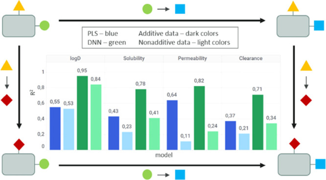
Figure 1.

R² and RMSE for log D and clearance—Set 3 (only additive data) vs Set 4 (only nonadditive data). Comparison of different models and endpoints. R_max² (dashed line) is the upper limit for R² derived from experimental uncertainty (Table 3). Full performance details can be found in the Supporting Information (SI Figures S6 and S7).

Figure 2.

R² against RMSE for test (a) Set 3 (only additive data) and (b) Set 4 (only nonadditive data). Comparison of different models and endpoints.

The analysis of R² and RMSE shows the same accuracy ranking for all models when comparing different data sets: Set 3 > Set 2 > Set 1 > Set 4. This is valid for all properties considered in this work with the exception of log D modeled using PLS and SVR. Predictive models are most accurate for additive data sets (Set 3) while nonadditive data (Set 4) are least well predictable (SI Figures S6 and S7). Mixed data sets with both additive and nonadditive data (Set 1 and Set 2) are ranked in the middle. There is just a small difference in R² and RMSE values between Set 1 (all data) and Set 3 (MMPs), indicating that using only MMPs instead of all datapoints does not improve the models significantly.

Figure 1 shows the comparison of performance metrics for additive vs nonadditive data for log D and clearance (Set 3 and Set 4). In most cases, deep learning algorithms give the best results (lowest RMSE and highest R²) followed by XGBoost and RF. The worst performance is observed for the linear model PLS, which serves as a benchmark.

Deep learning models based on additive data achieve for log D predictions almost R_max², which is calculated based on experimental uncertainty. For clearance, the achieved performance on the additive test set is significantly lower than R_max. For all properties, the performances of all models drop when applied to nonadditive data. The only exception is the SVR model based on nonadditive log D data, with an increase in R² from 0.58 to 0.74 for additive and nonadditive data, respectively (SI Figures S6 and S7). Log D is the property for which the performance is least affected with both DNN models achieving R² of 0.84 when trained on nonadditive data only. For solubility, permeability and clearance models based on nonadditive data only achieve R² < 0.43.

In terms of the deep learning models, multitask modeling improves over single-task for all studied properties except for log D. More hyperparameter trial settings (20 compared to 50) improve the models only slightly and remain below the performance of multitask models (DNN-S_20 and DNN-S_50 in Tables 5 and 6).

Figure 2 displays the correlation between R² and RMSE and shows different slopes for each property trendline. The lowest RMSE and R² are for clearance, while the highest for log D, with permeability and solubility being placed in between. For most properties, the correlation between R² and RMSE is linear, with some variation observed for log D Set 3 (only additive data).

Comparison between additive and nonadditive data (Table 5 and Figure 2) reveals that even deep learning methods, which are nonlinear, have problems with nonadditivity. It can be clearly seen in Figure 2 that only for log D the R² range is similar for additive and nonadditive data, while for the other properties it is shifted toward lower values (below 0.45). Log D is a bulk property and should therefore be less impacted by nonadditivity. The observed nonadditivity might be the result of random experimental errors. For the rest of the studied properties, many factors can introduce nonadditivity, like crystal packing in case of solubility and efflux, sticking to the membranes, and metabolism for cell-based properties (permeability and clearance) among others. The aim of this paper, however, is not to disclose the underlying reason for nonadditivity, but to recognize its importance, as models built on data sets with nonadditivity included lead to reduced predictability.

Figure 3 displays the correlation between measured and predicted solubility values using RF and a deep learning model (DNN-S_20) for additive and nonadditive data. As expected, the deep learning model performs generally better than RF. This improved performance is observed throughout the whole range of values, for all data sets and properties (SI Figures S8–S10). We performed a zero-slope analysis using the t-test (see Tables S3 and S4 and details in the SI) to check the significance of R². For all properties, P-values are below the significance level indicating that R² obtained in our analysis is statistically significant.

Figure 3.

Predicted versus measured values for solubility. Comparison between RF (left column) and DNN-S_20 (right column) for Set 3: only additive data (blue) and Set 4: only nonadditive data (orange). The values are in log units.

Conclusions

In this publication, we have evaluated the implications of MMPs and (non-)additivity on machine learning and deep learning models. We hypothesized that due to the small molecular changes captured in MMPs, these should be easier to predict than non-MMPs. As expected, data sets with only additive datapoints are easiest to predict, as opposed to data sets with only nonadditive datapoints. Mixed data sets with both additive and nonadditive data are ranked in the middle. The sole reduction from all datapoints to MMPs only does not lead to a significant increase in predictability. Using only additive data thus leads to an improvement.

Comparison among properties shows the best performance for log D followed by solubility, permeability, and clearance. This is in accordance with the complexity of the physicochemical property. In terms of models, deep learning methods give the best results with lowest RMSE and highest R². However, our study indicates that even deep learning algorithms have problems with nonadditivity. This highlights the importance of recognition of nonadditive events before building a QSAR/ML model. Unfortunately, NA analysis is not included in a predictive modeling workflow on a regular basis. We strongly advocate that this step becomes best practice, as the quality of model and the prediction error depend on nonadditive data. This would also allow more relevant comparisons of different models with similar endpoints, but based on different data sets with additive compounds. Moreover, identification and analysis of nonadditive effects are important, as they reveal critical changes in the SAR and are therefore the most interesting from a medicinal chemistry perspective.

Data and Software Availability

Data

Data underlying the findings described in this manuscript are considered proprietary to AstraZeneca and are not publicly available. The reason why we have used our internal database for this work, instead of public data, is that we needed to have assay consistency and enough nonlinear datapoints in order to test our hypothesis. Based on our recent publication “Nonadditivity in public and inhouse data: implications for drug design”⁴ we have shown that our internal AZ database contains more nonlinear events than the public database. Moreover, the assay data are more consistent in the AZ database. We strongly believe that the trends presented here are reproductible observations and general issues with QSAR models.

Software

The software used in this work is available on GitHub:

• https://github.com/MolecularAI/NonadditivityAnalysis (Jupyter notebook used for data preparation and NA analysis).

• https://github.com/KramerChristian/NonadditivityAnalysis (nonadditivity analysis code was made available by Christian Kramer).

• https://github.com/rdkit/mmpdb (matched molecular pair generation code was made available by Andrew Dalke).

• https://github.com/MolecularAI/Qptuna & https://github.com/MolecularAI/MMP_project (partial least squares (PLS), random forest (RF), support vector regressor (SVR), and gradient-boosted trees (XGBoost) models were build using QPTUNA).

• https://github.com/chemprop/chemprop (deep learning models were build using the directed message passing neural network (D-MPNN)).

Glossary

Abbreviations

NA

nonadditivity

AZ

AstraZeneca

SAR

structure–activity relationship

QSAR

quantitative structure–activity relationship

ML

machine learning

MMP

matched molecular pair

PLS

partial least squares

RF

random forest

SVR

support vector regressor.

Supporting Information Available

The Supporting Information is available free of charge at https://pubs.acs.org/doi/10.1021/acsomega.2c02738.

• Additional figures and tables: conversion for properties; test scores for cross-validation; zero-slope analysis; workflow of the whole study; determination of experimental uncertainty; and comparison between RF and DNN methods for additive and nonadditive data (PDF)

Author Present Address

^§ Data Science Department, Odyssey Therapeutics, Cambridge, Massachusetts, United States (C.M.)

Author Contributions

^∥ K.K. and E.N. are shared first authors.

Author Contributions

E.N. and K.K. performed data curation. N.A. analyzed and wrote the paper. J.H., C.M., and A.V. realized the M.L. study. C.T. supervised the study and wrote the paper. All authors read and approved the final manuscript.

The authors declare no competing financial interest.

References

- Ehmki E. S. R. R.; Kramer C. Matched Molecular Series: Measuring SAR Similarity. J. Chem. Inf. Model. 2017, 57, 1187–1196. 10.1021/acs.jcim.6b00709. [DOI] [PubMed] [Google Scholar]
- Tyrchan C.; Evertsson E. Matched Molecular Pair Analysis in Short: Algorithms, Applications and Limitations. Comput. Struct. Biotechnol. J. 2017, 15, 86–90. 10.1016/j.csbj.2016.12.003. [DOI] [PMC free article] [PubMed] [Google Scholar]
- Awale M.; Riniker S.; Kramer C. Matched Molecular Series Analysis for ADME Property Prediction. J. Chem. Inf. Model. 2020, 60, 2903–2914. 10.1021/acs.jcim.0c00269. [DOI] [PubMed] [Google Scholar]
- Gogishvili D.; Nittinger E.; Margreitter C.; Tyrchan C. Nonadditivity in Public and Inhouse Data: Implications for Drug Design. Aust. J. Chem. 2021, 13, 47. 10.1186/s13321-021-00525-z. [DOI] [PMC free article] [PubMed] [Google Scholar]
- Dimova D.; Bajorath J. Advances in Activity Cliff Research. Mol. Inform. 2016, 35, 181–191. 10.1002/minf.201600023. [DOI] [PubMed] [Google Scholar]
- Dimova D.; Heikamp K.; Stumpfe D.; Bajorath J. Do Medicinal Chemists Learn from Activity Cliffs? A Systematic Evaluation of Cliff Progression in Evolving Compound Data Sets. J. Med. Chem. 2013, 56, 3339–3345. 10.1021/jm400147j. [DOI] [PubMed] [Google Scholar]
- Hu H.; Bajorath J. Introducing a New Category of Activity Cliffs Combining Different Compound Similarity Criteria. RSC Med. Chem. 2020, 11, 132–141. 10.1039/C9MD00463G. [DOI] [PMC free article] [PubMed] [Google Scholar]
- Kramer C.; Fuchs J. E.; Liedl K. R. Strong Nonadditivity as a Key Structure–Activity Relationship Feature: Distinguishing Structural Changes from Assay Artifacts. J. Chem. Inf. Model. 2015, 55, 483–494. 10.1021/acs.jcim.5b00018. [DOI] [PMC free article] [PubMed] [Google Scholar]
- Gomez L.; Xu R.; Sinko W.; Selfridge B.; Vernier W.; Ly K.; Truong R.; Metz M.; Marrone T.; Sebring K.; Yan Y.; Appleton B.; Aertgeerts K.; Massari M. E.; Breitenbucher J. G. Mathematical and Structural Characterization of Strong Nonadditive Structure–Activity Relationship Caused by Protein Conformational Changes. J. Med. Chem. 2018, 61, 7754–7766. 10.1021/acs.jmedchem.8b00713. [DOI] [PubMed] [Google Scholar]
- Baum B.; Muley L.; Smolinski M.; Heine A.; Hangauer D.; Klebe G. Non-Additivity of Functional Group Contributions in Protein–Ligand Binding: A Comprehensive Study by Crystallography and Isothermal Titration Calorimetry. J. Mol. Biol. 2010, 397, 1042–1054. 10.1016/J.JMB.2010.02.007. [DOI] [PubMed] [Google Scholar]
- Schönherr H.; Cernak T. Profound Methyl Effects in Drug Discovery and a Call for New C-H Methylation Reactions. Angew. Chem. Int. Ed. 2013, 52, 12256–12267. 10.1002/anie.201303207. [DOI] [PubMed] [Google Scholar]
- Leung C. S.; Leung S. S. F.; Tirado-Rives J.; Jorgensen W. L. Methyl Effects on Protein–Ligand Binding. J. Med. Chem. 2012, 55, 4489–4500. 10.1021/jm3003697. [DOI] [PMC free article] [PubMed] [Google Scholar]
- Liu Y.; Bi M.; Zhang X.; Zhang N.; Sun G.; Zhou Y.; Zhao L.; Zhong R. Machine Learning Models for the Classification of CK2 Natural Products Inhibitors with Molecular Fingerprint Descriptors. Processes 2021, 9, 2074. 10.3390/pr9112074. [DOI] [Google Scholar]
- Rodríguez-Pérez R.; Bajorath J. Multitask Machine Learning for Classifying Highly and Weakly Potent Kinase Inhibitors. ACS Omega 2019, 4, 4367–4375. 10.1021/acsomega.9b00298. [DOI] [Google Scholar]
- Yang M.; Tao B.; Chen C.; Jia W.; Sun S.; Zhang T.; Wang X. Machine Learning Models Based on Molecular Fingerprints and an Extreme Gradient Boosting Method Lead to the Discovery of JAK2 Inhibitors. J. Chem. Inf. Model. 2019, 59, 5002–5012. 10.1021/acs.jcim.9b00798. [DOI] [PubMed] [Google Scholar]
- Wu Z.; Ramsundar B.; Feinberg E. N.; Gomes J.; Geniesse C.; Pappu A. S.; Leswing K.; Pande V. MoleculeNet: A Benchmark for Molecular Machine Learning. Chem. Sci. 2018, 9, 513. 10.1039/c7sc02664a. [DOI] [PMC free article] [PubMed] [Google Scholar]
- Mayr A.; Unter Klambauer G.; Unterthiner T.; Steijaert M.; Wegner J. O. K.; Ceulemans H.; Arn D.-A.; Clevert A.; Hochreiter S. Large-Scale Comparison of Machine Learning Methods for Drug Target Prediction on ChEMBL. Chem. Sci. 2018, 9, 5441. 10.1039/c8sc00148k. [DOI] [PMC free article] [PubMed] [Google Scholar]
- Coley C. W.; Barzilay R.; Green W. H.; Jaakkola T. S.; Jensen K. F. Convolutional Embedding of Attributed Molecular Graphs for Physical Property Prediction. J. Chem. Inf. Model. 2017, 57, 1757–1772. 10.1021/acs.jcim.6b00601. [DOI] [PubMed] [Google Scholar]
- Chithrananda S.; Grand G.; Ramsundar B.. ChemBERTa: Large-Scale Self-Supervised Pretraining for Molecular Property Prediction. arXiv:2010.09885 2020, 10.48550/arxiv.2010.09885. [DOI] [Google Scholar]
- Wang S.; Guo Y.; Wang Y.; Sun H.; Huang J.. Smiles-Bert: Large Scale Unsupervised Pre-Training for Molecular Property Prediction. In ACM-BCB 2019 - Proceedings of the 10th ACM International Conference on Bioinformatics, Computational Biology and Health Informatics; ACM, 2019; pp. 429–436. [Google Scholar]
- Wang Y.; Wang J.; Cao Z.; Farimani A. B. Molecular Contrastive Learning of Representations via Graph Neural Networks. Nat. Mach. Intell. 2022, 4, 279–287. 10.1038/s42256-022-00447-x. [DOI] [Google Scholar]
- Rong Y.; Bian Y.; Xu T.; Xie W.; Wei Y.; Huang W.; Huang J.. Self-Supervised Graph Transformer on Large-Scale Molecular Data. Adv. Neural Inf. Process. Syst. arXiv:2007.02835, 2020, 10.48550/arxiv.2007.02835. [DOI] [Google Scholar]
- Fang X.; Liu L.; Lei J.; He D.; Zhang S.; Zhou J.; Wang F.; Wu H.; Wang H. Geometry-Enhanced Molecular Representation Learning for Property Prediction. Nat. Mach. Intell. 2022, 4, 127–134. 10.1038/s42256-021-00438-4. [DOI] [Google Scholar]
- Yang K.; Swanson K.; Jin W.; Coley C.; Eiden P.; Gao H.; Guzman-Perez A.; Hopper T.; Kelley B.; Mathea M.; Palmer A.; Settels V.; Jaakkola T.; Jensen K.; Barzilay R. Analyzing Learned Molecular Representations for Property Prediction. J. Chem. Inf. Model. 2019, 59, 3370–3388. 10.1021/ACS.JCIM.9B00237. [DOI] [PMC free article] [PubMed] [Google Scholar]
- Kramer C.; Kalliokoski T.; Gedeck P.; Vulpetti A. The Experimental Uncertainty of Heterogeneous Public K i Data. J. Med. Chem. 2012, 55, 5165–5173. 10.1021/jm300131x. [DOI] [PubMed] [Google Scholar]
- Kalliokoski T.; Kramer C.; Vulpetti A.; Gedeck P. Comparability of Mixed IC50 Data - A Statistical Analysis. PLoS One 2013, 8, e61007 10.1371/journal.pone.0061007. [DOI] [PMC free article] [PubMed] [Google Scholar]
- Kramer C. Nonadditivity Analysis. J. Chem. Inf. Model. 2019, 59, 4034–4042. 10.1021/acs.jcim.9b00631. [DOI] [PubMed] [Google Scholar]
- Dalke A.; Hert J.; Kramer C. Mmpdb: An Open-Source Matched Molecular Pair Platform for Large Multiproperty Data Sets. J. Chem. Inf. Model. 2018, 58, 902–910. 10.1021/acs.jcim.8b00173. [DOI] [PubMed] [Google Scholar]
- Sheridan R. P.; Karnachi P.; Tudor M.; Xu Y.; Liaw A.; Shah F.; Cheng A. C.; Joshi E.; Glick M.; Alvarez J. Experimental Error, Kurtosis, Activity Cliffs, and Methodology: What Limits the Predictivity of Quantitative Structure-Activity Relationship Models?. J. Chem. Inf. Model. 2020, 60, 1969–1982. 10.1021/acs.jcim.9b01067. [DOI] [PubMed] [Google Scholar]
- Landrum G.RDKit: Open-Source Cheminformatics, 2006.
- Hussain J.; Rea C. Computationally Efficient Algorithm to Identify Matched Molecular Pairs (MMPs) in Large Data Sets. J. Chem. Inf. Model. 2010, 50, 339–348. 10.1021/ci900450m. [DOI] [PubMed] [Google Scholar]
- Akiba T.; Sano S.; Yanase T.; Ohta T.; Koyama M.. Optuna: A Next-Generation Hyperparameter Optimization Framework. In Proceedings of the ACM SIGKDD International Conference on Knowledge Discovery and Data Mining; Association for Computing Machinery: New York, NY, USA, 2019; pp. 2623–2631. [Google Scholar]
- Gilmer J.; Schoenholz S. S.; Riley P. F.; Vinyals O.; Dahl G. E.. Neural Message Passing for Quantum Chemistry. In Proceedings of the 34th International Conference on Machine Learning; PMLR, 2017; 70, pp. 1263-1272. [Google Scholar]
- Bergstra J.; Yamins D.; Cox D. D.. Making a Science of Model Search: Hyperparameter Optimization in Hundreds of Dimensions for Vision Architectures. In Proceedings of the 30th International Conference on Machine Learning; PMLR, 2013; Vol. 28, pp. 115-123. [Google Scholar]
Associated Data
This section collects any data citations, data availability statements, or supplementary materials included in this article.
Supplementary Materials
Data Availability Statement