Deep learning-enabled assessment of cardiac allograft rejection from endomyocardial biopsies

Abstract

Endomyocardial biopsy (EMB) screening represents the standard-of-care for detecting allograft rejections after heart transplant. Manual interpretation of EMBs is affected by substantial inter-and-intraobserver variability, which often leads to inappropriate treatment with immunosuppressive drugs, unnecessary follow-up biopsies, and poor transplant outcomes. Here we present a deep learning-based artificial intelligence (AI) system for automated assessment of gigapixel whole-slide images obtained from EMBs, which simultaneously addresses detection, subtyping, and grading of allograft rejection. To assess model performance, we curated a large dataset from the USA as well as independent test cohorts from Turkey and Switzerland, which together include large-scale variability across populations, sample preparations, and slide scanning instrumentation. The model detects allograft rejection with an AUC of 0.962, assesses the cellular and antibody-mediated rejection type with AUCs of 0.958 and 0.874, respectively, detects Quilty-B lesions, benign mimics of rejection, with an AUC of 0.939, and differentiates between low- and high-grade rejections with an AUC of 0.833. In a human reader study, the AI-system provided non-inferior performance to conventional assessment and reduced inter-rater variability and assessment time. This robust evaluation of cardiac allograft rejection paves the way for clinical trials to establish the efficacy of AI-assisted EMB assessment and its potential for improving heart transplant outcomes.

Cardiac failure is a leading cause of hospitalization in the United States and the most rapidly growing cardiovascular condition globally[1, 2]. For patients with end-stage heart failure, transplantation often represents the only viable solution[3]. Cardiac allograft transplantation is associated with significant risk of rejection, affecting 30–40% of recipients mainly within the first six months after transplantation[4]. To reduce the incidence of rejection, patients receive individually tailored immunosuppressive regimens after transplantation. Despite the medications, cardiac rejection remains the most common and serious complication, as well as the main cause of mortality in post-transplantation patients[5–8].

Since early stages of rejections may be asymptomatic[8], patients undergo surveillance endomyocardial biopsies (EMBs) typically starting days to weeks after transplantation. Although there is no standard schedule, most centers perform frequent biopsies for 1–2 years. Thereafter, the frequency is center-specific or on a for-cause basis. The gold-standard for EMB evaluation consists of manual histologic examination of hematoxylin and eosin (H&E)-stained tissue[3]. EMB assessment includes detection and subtyping of rejection as acute-cellular rejection (ACR), antibody-mediated rejection (AMR), or concurrent cellular-antibody rejections, in addition to the identification of benign mimickers of rejections. The severity of the rejection is further characterized by grade. The rejection subtype and grade govern treatment regimen and patient management. Despite several revisions to the official guidelines, the interpretation of the EMBs remains challenging with limited inter- and intra-observer reproducibility [9–11]. Overestimation of rejection can lead to increased patient anxiety, over-treatment, and unnecessary follow-up biopsies, while underestimation may lead to delays in treatment and ultimately worse outcomes.

Deep learning-based, objective and automated assessment of EMBs can help mitigate these challenges, potentially improving reproducibility and transplant outcomes. Multiple studies have demonstrated the potential of AI-models to reach performance comparable or even superior to human experts in various diagnostic tasks[12–24]. Previous attempts to algorithmically assess EMBs are limited to small datasets of manually extracted region of interests (ROIs) or hand-crafted features, did not focus on all tasks involved in EMB assessment, and lacked rigorous international validation across different patient populations[25–28].

In this study, we present Cardiac Rejection Assessment Neural Estimator (CRANE), a deep-learning approach for cardiac allograft rejection screening in H&E-stained whole-slide images (WSIs). CRANE addresses all major diagnostic tasks: rejection detection, subtyping, grading, and also detection of Quilty-B lesions. CRANE is trained with thousands of gigapixel whole slide images using case-level labels, supporting seamless scalability to large datasets without the burden of manual annotations. The model performance is evaluated on three test cohorts from the USA, Turkey, and Switzerland, using different biopsy protocols and scanner instrumentation. For model interpretability and introspection, visual representation of the model predictions are obtained via high-resolution heatmaps, reflecting the diagnostic relevance of morphologic regions within the biopsy. An independent reader study is performed to assess the model’s consensus with manual expert assessment and to demonstrate the potential of AI-assistance in reducing inter-rater variability and assessment time. An overview of the study is shown in Figure 1.

Figure 1: Cardiac Rejection Assessment Neural Estimator (CRANE) workflow.

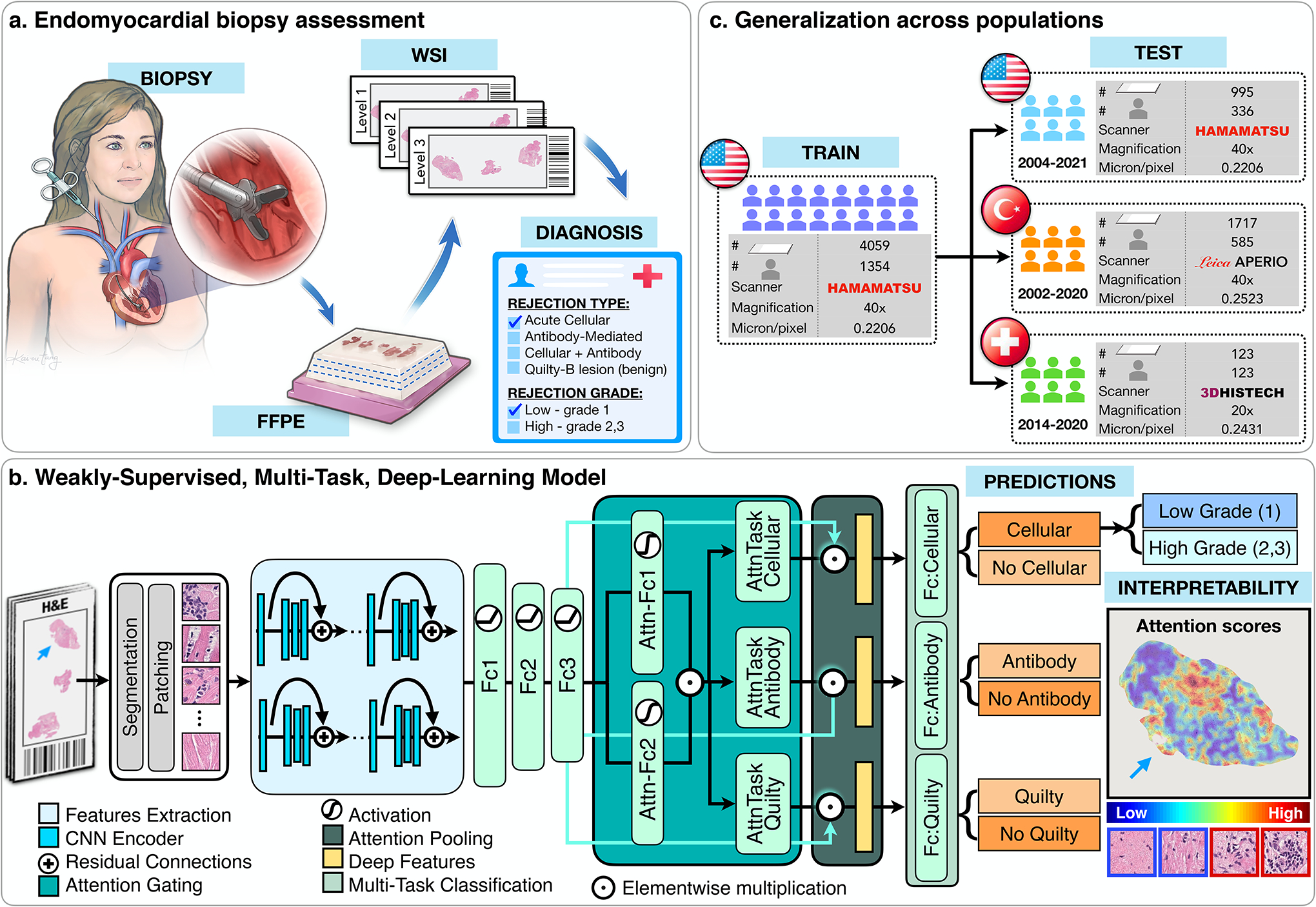
a. Fragments of endomyocardial tissue are formalin fixed and paraffin embedded (FFPE). Each paraffin block is cut into slides with three consecutive levels and stained with H&E. Each slide is digitized and served as an input for the model. b. CRANE first segments tissue regions in the WSI and patches them into smaller sections. Pretrained encoder was used to extract features from the image patches, which are further fine-tuned through a set of three fully-connected layers, marked as Fc1, Fc2, and Fc3. A weakly supervised multi-task, multi-label network was constructed to simultaneously identify normal tissue and different rejection conditions (cellular, antibody, and/or Quilty-B lesions). The attention scores, reflecting relevance of each image region towards the model prediction, can be visualized in the form of whole-slide attention heatmaps. c. The model was trained on the USA cohort, using 70% cases for training and 10% for validation and model selection. Evaluation of the model was conducted on the internal USA dataset using the remaining held-out 20% cases and two external cohorts from Turkey, and Switzerland. Detailed breakdown of these datasets is presented in Supplemental Table 1.

Results

Endomyocardial Biopsy Assessment via Deep Learning

CRANE is developed on an internal dataset consisting of 5,054 gigapixel WSIs from 1,690 patient biopsies collected from the Brigham and Women’s Hospital. Each biopsy had three WSIs representing three levels of the tissue block (Figure 1a). Each case has associated labels for the presence of rejection, characterization of the rejection type as cellular and/or antibody-mediated, rejection grade, and presence of Quilty-B lesion. All cases diagnosed as AMRs were confirmed with C4d immunohistochemical (IHC) staining. The internal dataset was used for model training, validation, and held-out testing. To rigorously assess model adaptability, CRANE was tested on two additional independent international cohorts sourced from Turkey (1,717 WSIs from 585 patients) and Switzerland (123 WSIs from 123 patients). These independent international test sets were deliberately constructed to reflect the large data variability present across populations and medical centers; including different biopsy protocols, slide preparation mechanisms, and different scanner vendors, which are all known contributors to image variability[17, 18, 35]. The variation in the color distribution across cohorts is illustrated in Extended Data Fig. 1. A specification of the data collection protocols, and the patient cohorts are provided in Figure 1, Supplemental Table 1, and the Dataset Description section of Methods.

CRANE is a high-throughput, multi-task framework that simultaneously detects ACR, AMR, and Quilty-B lesions, including their concurrent appearances using H&E-stained WSIs as the input (Figure 1b). Due to the large size of gigapixel histology images, it is computationally inefficient and usually not possible to apply deep-learning models directly to the WSI. To circumvent this, we first automatically segment tissue regions and patch them into smaller sections. Using transfer learning, a deep residual convolutional neural network (CNN) is deployed as an encoder to extract low-dimensional features from raw image patches. The extracted features are further tuned to histology-specific representations through a fully-connected neural network. This allows for a high dimensional gigapixel WSI to be embedded into a set of compact low-dimensional feature vectors for efficient training and inference. The feature vectors serve as input for the attention-based multiple instance learning (MIL) module[17, 36]. Using the patient diagnoses for the supervision, the attention module learns to rank the relative importance of each biopsy region towards the determination of each classification task. The parameters in the first attention layers are shared among all three tasks to enable the identification of atypical myocardial tissue. Subsequently, a separate branch is used for each task, allowing the model to identify morphology specific to each diagnosis. The feature representations from all tissue patches, weighted by their respective predicted attention score for each task, are aggregated in attention pooling[36]. The resulting slide-level features are then evaluated by the corresponding task-specific classifier, which independently determines the presence or absence of ACR, AMR, and Quilty-B lesions, respectively. The presence of overall rejection is obtained by combining the AMR and ACR predictions for each biopsy. A separate, single-task MIL classifier is trained to determine the grade for each detected rejection, discriminating between low grade (grade-1) and high grade (grade-2 and 3) cases. The grade-2 and 3 are combined into a single group since they both require treatment interventions, in contrast to observational strategy used in grade-1 rejections, as well as due to the extremely low appearance of grade-3 cases. The high-grade rejection are then further differentiated into the specific sub-grades using a separate network. Due to the extremely rare occurrence of grade 3 rejections (9 cases in the USA, 13 in the Turkish, and none in the Swiss cohort), this problem could not be addressed at the whole-slide-level (i.e. using the weakly-supervised approach). Instead, a supervised model is designed which uses pixel-level annotations. This model, summarized in Extended Data Fig. 2, is trained on patches extracted from the biopsy regions corresponding to the specific rejection grades as annotated by experts. Additional details on the model architecture and hyper-parameters are described in the Methods section.

Evaluation of Model Performance

The internal USA dataset is partitioned into 70/10/20% splits for training, validation, and held out testing, respectively. The partition is constructed in a way to ensure a balanced proportion of each diagnosis across all splits. Multiple slides from the same biopsy are always presented in the same split. The model training is performed on slide-level, where each slide is considered as an independent data point with patient diagnoses as labels.

We examined the model performance across different magnifications, including 40x, 20x, and 10x. These experiments show that the rejections and Quilty-B lesions are best estimated by fusion of models across multiple magnification, while the best performance for the grade prediction was achieved at 10x magnification (Extended Data Fig. 3a,b). This observation is compatible with the manual assessment, where signs of rejections usually need to be examined at different magnifications, while lower magnification is more informative for the grade determination since it provides more context on the extent of myocardial injury. Learning curves for all tasks are shown in Extended Data Fig. 3c.

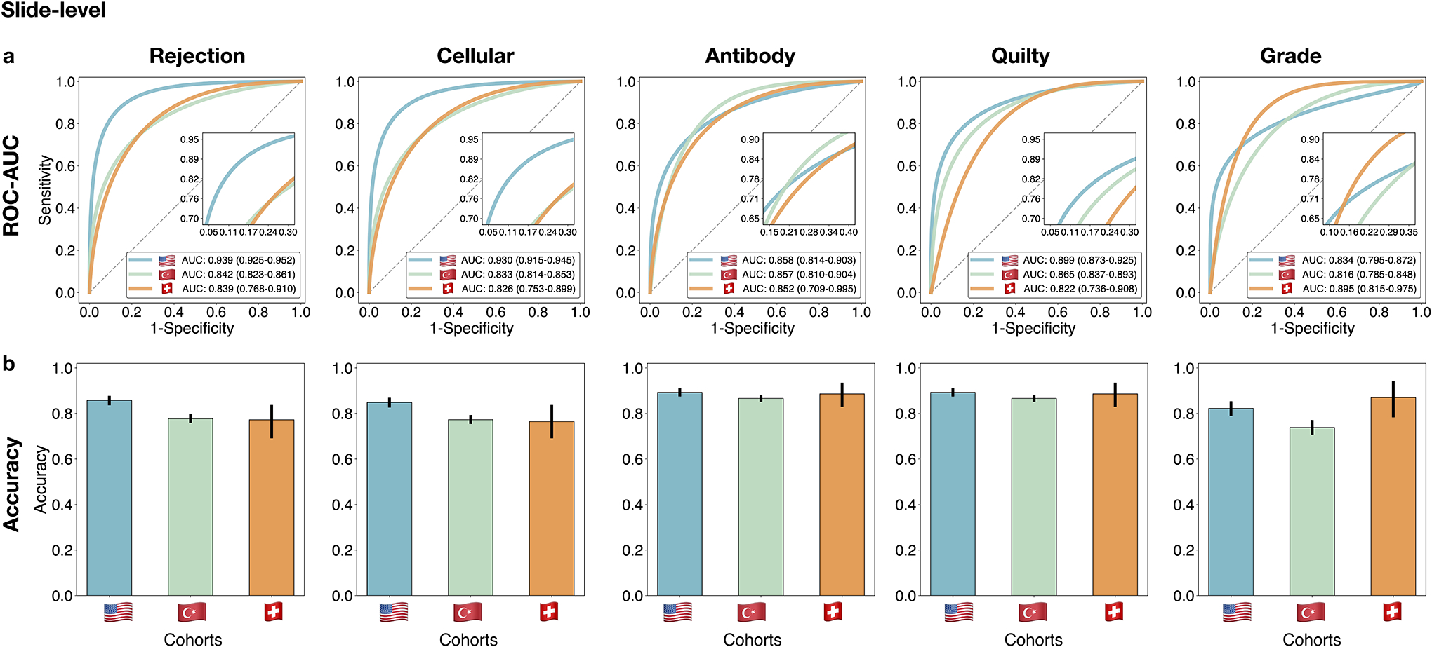
On the held-out USA test set, which was not seen by the model during training, the model accuracy (ACC) and area under receiver operating characteristic curve (AUC) at the patient-level are as follows: cellular rejections - AUC=0.958 (95% CI: 0.940–0.977), ACC=0.893, antibody-mediated rejection - AUC=0.874 (95% CI:0.801–0.946), ACC=0.899, Quilty-B lesions - AUC=0.939 (95% CI:0.910–0.969), ACC=0.920, and grade AUC=0.833 (95% CI: 0.764–0.901), ACC=0.818, while the performance for overall rejection detection reached AUC of 0.962 (95% CI: 0.943–0.980) and an accuracy of 0.899. The patient/biopsy-level performance is reported in Figure 2 and Supplemental Table 2 and slide-level scores are provided in Extended Data Fig. 4, Supplemental Tables 3 and 4. The high performance in detecting overall rejections implies the model’s potential for screening negative cases. CRANE is also able to differentiate between ACR and their benign mimickers, Quilty-B lesions. Other benign injuries, such as old biopsy sites, focal healing injuries, and tissue scars, can often imitate the appearance of ACRs, particularly in the early stages after transplantation[37]. Although the model was not explicitly trained to account for such injuries, it learned to differentiate between ACRs and early injuries (i.e. 6 months post-transplant) with AUC of 0.983 (95 % CI: 0.950–1.00), and an AUC of 0.977 (% CI 0.963–0.991) for both early and old injuries (Supplemental Table 5). The also model is able to identify AMR using conventional H&E stained slides which is in line with other recent studies demonstrating the potential of deep-learning models to infer certain IHC properties from the H&E slides alone[34, 38]. In comparison to other tasks, the model performance is lower for the rejection grading, similar to the trends observed in manual EMB assessment[9–11]. This can be attributed to the higher complexity of the grading task over rejection detection since the grade is characterized by the type and also extent of the tissue injury. The high-grade ACRs were further refined into the respective grades (i.e. grade 2 vs 3) through the supervised grading model (see Methods), which achieved an AUC of 0.929 (95% CI: 0.861–0.997) and ACC= 0.885 at the patch-level (Extended Data Fig. 2). For slide-level predictions, obtained by the fusion of the patch-level estimates through a majority voting, were obtained with AUC=0.960 and ACC=0.800 (Supplemental Table 6).

Figure 2: Performance of the CRANE model at patient-level.

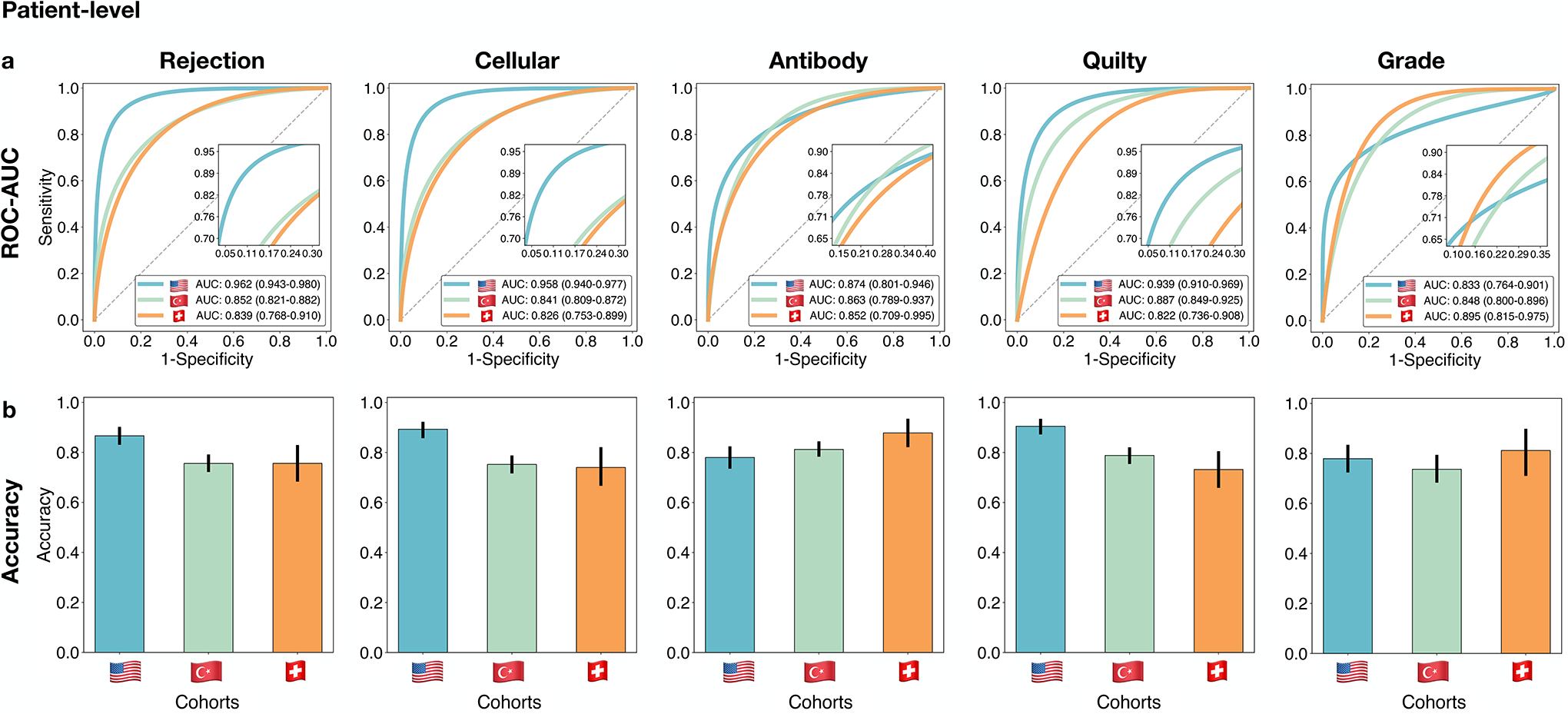
The CRANE model was evaluated on the test set from the USA (n=995 WSIs, N=336 patients) and two independent external cohorts from Turkey (n=1,717, N=585), and Switzerland (n=123, N=123). a. Receiver operating characteristic (ROC) curves for the multitask classification of EMB evaluation and grading at the patient-level. The area under the ROC curve (AUC) is reported together with the 95% confidence intervals (CIs) for each cohort. b. The bar plots reflect the model accuracy for each task. Error bars (marked by the black lines) indicate 95% CIs and the center is always the computed value for each cohort (specified by the respective axis labels).

The performance of the model is comparable for slide-level and patient/biopsy-level predictions. These results further imply that the patient-level labels, which are readily available in clinical records, are sufficient for model training without the burden of assigning diagnoses for each slide separately. While there may be label noise in the training data due to observer variability, deep learning models are known to be robust to a substantial amount of label noise[39]. The model performance across different patient groups (Supplemental Tables 7 to 9) further illustrates the model robustness to variations in patient’s age, gender, and time since transplant. The model robustness can be also assessed through the confidence of the predictions as demonstrated in Extended Data Fig. 5.

Generalization to Independent International Test Cohorts

The AI-model is applied, without any form of domain adaptation, stain-normalization, or model tuning, to the two independent international external cohorts (Switzerland and Turkey). To stress-test the trained model these cohorts reflect large scale variability from the training cohort including different slide preparation protocols, and slide scanning vendors. Consistent with our assessment on the in-house held out dataset, the multitask model is applied to all available magnification downsamples in each cohort, while the grade is assessed from the 10x magnification. The patient-level scores are reported in Figure 2, Extended Data Fig. 6 and Supplemental Table 2, while the slide-level performance is reported in Extended Data Fig. 4 and Supplemental Tables 3 and 4. The scores for the refinement of the high-grade cellular rejections are reported in Extended Data Fig. 2 and Supplemental Table 6. Adapting the model from internal to external cohorts led to a drop in performance that varies between 0.02–0.13 for AUC and 0.02–0.14 for ACC scores, similar to other deep-learning models when applied to external independent data-sets[16, 18, 40]. The performance decrease can be attributed to the large data variations among the cohorts. As demonstrated by previous studies even small changes, such as re-scanning the same slides with different scanner and variation in the slide preparation can also reduce performance even on simple binary classification tasks[18]. Additional factors, such as different staining techniques, slide-thickens, micron-per-pixel (mpp) variations across scanners (even for the same resolution[17,35]), and signal-to-noise ratio are other known contributors affecting the model performance – all present in our cohorts. Despite the decrease in performance on the external dataset, the fact that the model reached comparable scores on two highly distinct international cohorts without any form of domain adaptation, implies the model’s ability to generalize across large variations presented in histopathology data. Assessment of model performance on patient subgroups (Supplemental Tables 7, 8, 9) further shows the model robustness to variations in patient’s age, gender, and time since transplant, which is especially interesting since the Turkey dataset also includes pediatric cases.

Model Interpretability

To visualize and interpret the model predictions, attention heatmaps can be generated for each task by mapping the normalized attention scores to their corresponding spatial location in the WSI, as shown in Figure 3 and in our public interactive demo available at http://crane.mahmoodlab.org. Technical details on heatmap generation are provided in the Methods. The attention scores represent the model interpretation of the diagnostic relevance of each biopsy region. While no manual annotations were used for training, the model has learned to discriminate between atypical and normal myocardial tissue. In all tasks, the high-attention regions typically correspond to diagnostically relevant morphology, while the low-attention scores are assigned to benign tissue. The attention maps should, however, not be over-interpreted as segmentation of rejection regions. They merely reflect the relative importance of each biopsy region (relative to others) for the model predictions. As so, we observed that the model places higher attention to the regions with atypical tissue, which might include even tissue without sign of rejection such as benign injuries or artifacts. The model predictions are, however, derived from the regions with the highest-attention scores for each task. This is further illustrated in Extended Data Fig. 7, which shows the attention heatmaps for a case with concurrent ACR, AMR, and Quilty-B lesion. Although at the slide-level view, the attention maps appear relatively similar for all three tasks, the highest attention regions correspond to tissue with the task-specific morphology. This example also provides a visual interpretation of the model ability to differentiate between ACR and similarly appearing Quilty-B lesions. There is a visible difference in the heatmap appearance between the rejection and grading task, the first being more refined and detailed, while the grading task heatmap has more coarse morphology. This observation is consistent with manual EMB examination, where fine morphological details are used to determine the rejection type, while grade evaluation requires more spatial context. The high-attention regions provide useful insights on the morphologies driving the model predictions. Further quantitative analysis showed a high agreement between the model and expert assessment of diagnostically relevant regions (Extended Data Fig. 8).

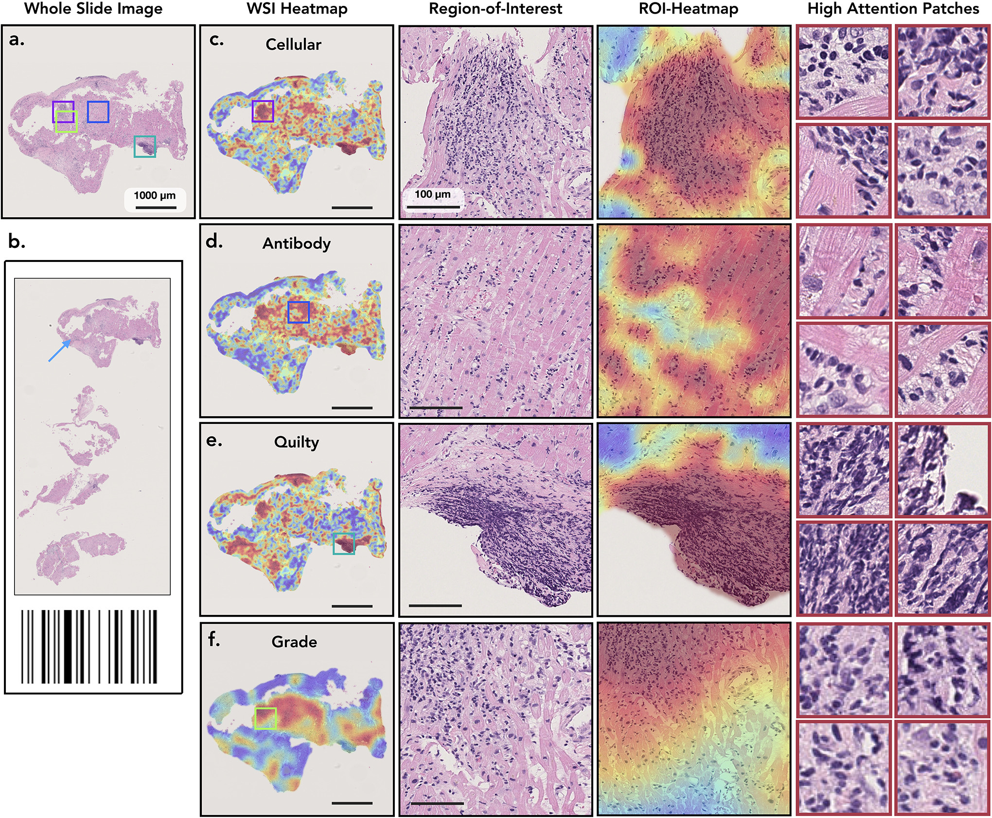
Figure 3: Visualisation of the attention heatmaps.

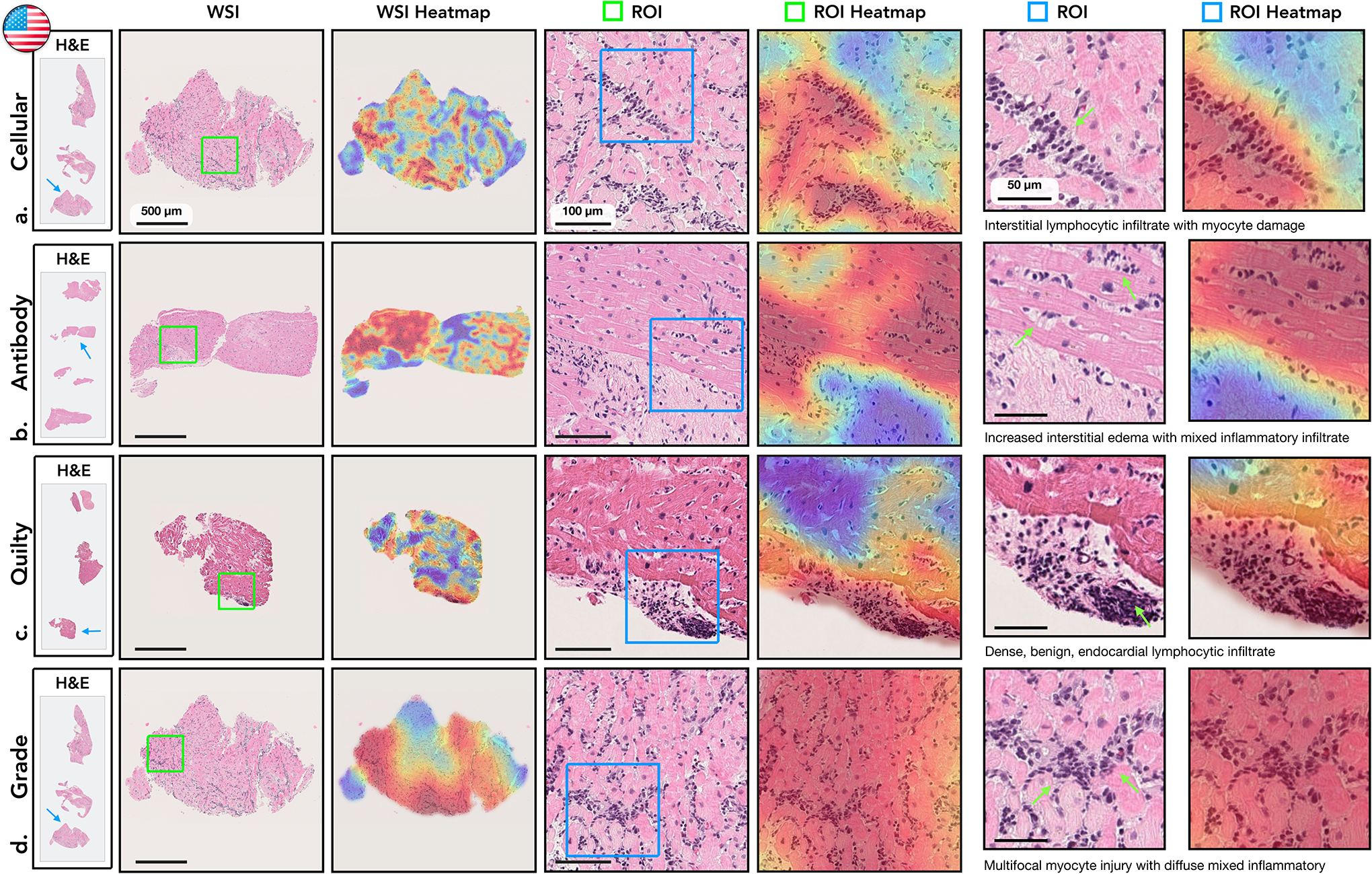
Sample of WSIs of EMBs with different diagnosis are shown in the first column. The second column displays a closer view to the cardiac tissue samples marked by blue arrows in the first column. An attention heatmap corresponding to each slide was generated by computing the attention scores for each predicted diagnosis (third column). A zoom-in-view of the regions of interest (ROIs) marked by green squares in the second column are shown in fourth column, while the corresponding attention heatmaps are displayed in the fifth column. The last two columns depict a zoom-in-view of the ROIs marked by the blue square together with the corresponding attention heatmap. Green arrows highlight specific morphology corresponding to the textual description. The colormap of the attention heatmaps range from red (high-attention) to blue (low-attention). a. Cellular Rejection. The highest attention scores identified regions with increased interstitial lymphocytic infiltrates and associated myocyte injury, while the adjacent, lower attention scores identified healthier myocytes without injury. b. Antibody-Mediated Rejection. The highest attention scores determined regions with edema within the interstitial spaces in addition to increased mixed inflammatory infiltrate, comprised of eosinophils, neutrophils, and lymphocytes. The adjacent lower attention scores identified background fibrosis, stroma, and healthier myocytes. c. Quilty-B Lesion. The highest attention scores distinguished a single, benign focus lymphocytes within the endocardium, without injury or damage to the myocardium. The lower attention scores correspond to background and healthy myocytes. d. Cellular Grade. The highest attentions identified diffuse, prominent interstitial lymphocytic infiltrates with associated myocyte injury, representing severe rejection. The lower attention regions identified background fibrosis and unaffected, healthier myocytes.

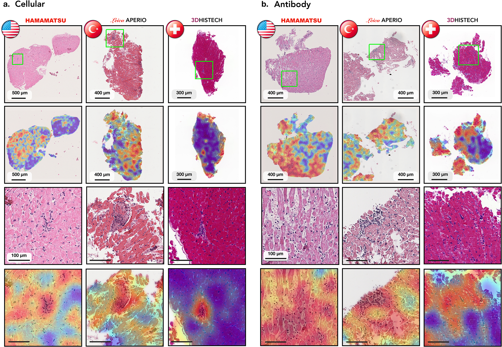
Attention heatmaps for the external datasets are presented in Figure 4. In all cohorts, the model strongly attended to regions with rejection morphology, while the low-attention scores were assigned to regions with normal or benign myocardial tissue. This further demonstrates the ability of the model to generalize across diverse populations and different scanners. To further investigate the model predictions and limitations, we performed a detailed analysis of failure cases. The top misclassified cases from each cohort, specifically the cases where the model made incorrect predictions with the highest confidence, are detailed in Figure 5. We observed that for all failure cases, the model has correctly assigned high attention scores to the regions with rejection morphology. The detection of the rejection regions, however, does not necessarily warrant correct predictions. It just implies that the model has considered these regions to be the diagnostically most relevant, however, the corresponding features might not be discriminative enough for the model to draw a correct prediction. Despite the incorrect predictions, the identified high-attention regions can guide pathologists towards the relevant biopsy regions and in turn reduce the inter- and intra-rater variability.

Figure 4: Analysis of attention-heatmaps in the three independent test cohorts.

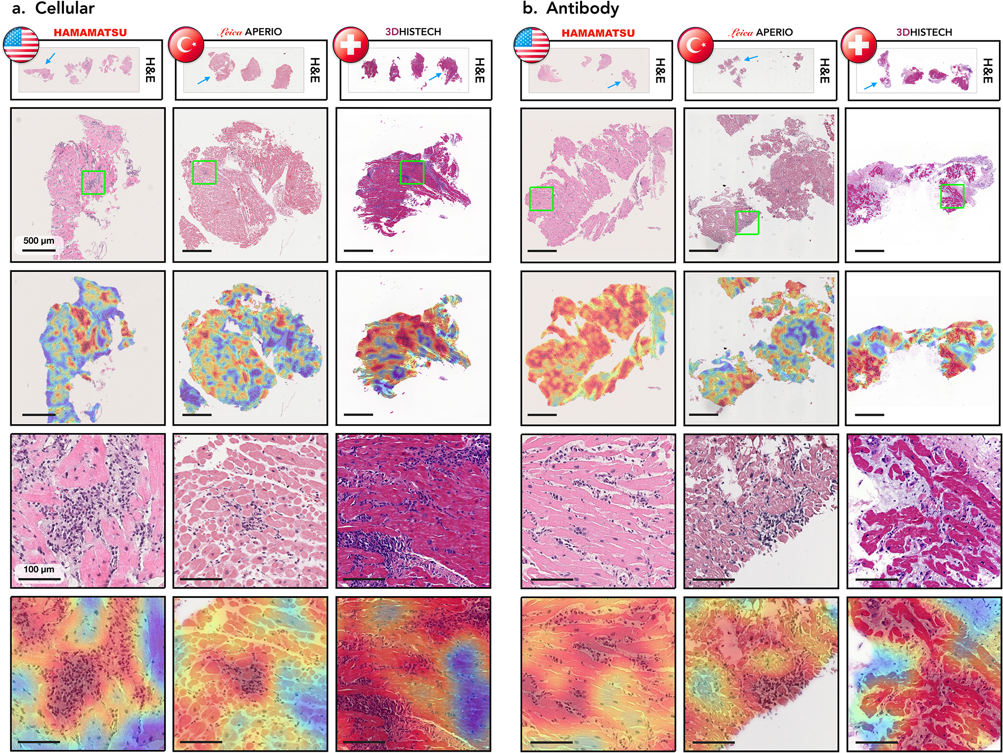
Displayed are cases with cellular (a.) and antibody-mediated rejections (b.) sourced from three cohorts: US (left columns), Turkish (middle columns), and Swiss (right columns). The types of scanners used for each cohort are indicated. The first row depicts WSIs from corresponding center, while the second row shows closer views on cardiac tissue samples marked by the blue arrows in the first row. The corresponding attention heatmaps are depicted in the third row. The colormap of the attention heatmaps range from red (high-attention) to blue (low-attention). The last two rows show a zoom-in-view of ROIs marked by the green squares in the second row along with the corresponding attention heatmaps.

Figure 5: Analysis of failure cases using attention heatmaps in the three independent test cohorts.

Displayed are cases with cellular (a.) and antibody mediated rejections (b.) which were incorrectly identified as normal by the model. Results are shown for the US (left columns), Turkish (middle columns), and Swiss (right columns) cohorts. The types of scanners used for each cohort are indicated. The WSIs from each center and the corresponding attention heatmap are shown in the first and the second row, respectively. The third row shows zoom-in-views in the ROIs marked by the green squares, while the accompanying attention heatmaps are shown in the last row.

Comparison with Human Readers

To compare the performance of the AI model with expert pathologists, we recruited five certified pathologists (average experience 10.5 years). Previous studies assessing the performance of AI models against pathologists for cancer diagnosis have relied on building a reference standard based on the consensus of human experts [15,16,19]. However, since the variability in EMB assessment is significantly large as compared to cancer diagnosis[11], cases where a consensus could be reached were relatively easy for the AI model. In light of this, we investigate the inter-observer variability among experts and the variability between the AI-system and individual experts. We randomly selected set of 150 EMBs from the Turkey cohort, including 91 ACR, 23 AMR cases (including 14 concurrent ACR and AMR cases), and 50 normal biopsies. All experts were blinded to pathology reports and previous assessments made on these biopsies. The cases were presented to the pathologists in random order through a digital web-based platform and no timing constraint was imposed on the readers. For evaluation purposes, the pathologists were asked to derive the diagnosis from H&E slides only, mimicking the CRANE’s set-up without the use of IHC for AMR detection. We first calculated the interobserver agreement between each pair of pathologists using Cohen’s kappa that takes into account agreement by chance and then calculated the agreement between individual expert pathologists and the CRANE model trained on US cases. The agreement between the five experts was comparable to previous studies for assessing interobserver agreement in EMBs[10]. For all tasks, we observed that the AI predictions are not inferior to the human reads (Extended Data Fig. 9). For example, the average agreement for rejection detection between individual pathologists was κ = 0.537 (moderate agreement) while the average agreement between individual pathologists and CRANE was κ = 0.639 (substantial agreement).

To further evaluate the potential of CRANE to serve as an assistive diagnostic tool, we conducted an additional reader study to assess the benefit of showing model generated heatmaps during case assessment. The pathologists were asked to assess 150 EMBs from the Turkey cohort. The readers were randomly asked to make assessments on WSIs only or on WSIs with AI-assistance in the form of attention-heatmaps shown as a semi-transparent layer at the top of H&E slide. All features available in our public interactive demo were available to the readers and no timing constraint was imposed on the readers. Following a four-week washout period, the pathologists repeated the task, but the readers from the first group used WSIs and the AI-assistance, while the second group used only WSIs. For the purpose of this study, we created the ground truth labels based on the consensus of the readers from the inter-rater variability experiment presented in Extended Data Fig. 9. While this reader study is limited in scope, it shows that utilizing CRANE as an assisting tool has increased the accuracy for all tasks and reduced the assessment time for all readers (shown in Extended Data Fig. 10). These results indicate the potential of AI-assistance in reducing the inter-rater variability and increasing the efficiency of manual biopsy assessment and set the stage for large scale studies and clinical trials to assess the benefit of AI-assisted EMB assessment.

Discussion

Herein, we present CRANE, a weakly-supervised deep-learning model for automated screening of EMBs in H&E-stained WSIs. Using multi-task learning, the model can simultaneously identify ACR, AMR, Quilty-B lesions, and their concurrent appearance, while an additional network is used to determine the rejection grade. The model has been trained using only patient diagnoses readily available in the clinical records, allowing seamless model deployment for large datasets from multiple centers. The usability of CRANE has been demonstrated on two independent international test cohorts, which reflect diverse geographic populations, scanners, and biopsy protocols. To the best of our knowledge, this is the first large-scale international validation of weakly-supervised computational pathology setup.

Although the datasets used in all three cohorts reflected the screening population of each participating institution, the proportion of AMRs cases was considerably lower in comparison to ACR in all cohorts, which is one limitation of the study. This can be attributed to the rarer appearance of AMRs and to the later recognition of this rejection type by the medical community. Even though CRANE’s performance for the rejection grading is comparable to human experts, this task remains challenging and might benefit from future model improvements.

Our model demonstrates the promise of AI-integration into the diagnostic workflow. However, optimal use of weakly-supervised models in clinical practice remains to be determined. The specific advantages of CRANE suggests its potential to act as an assistive diagnostic tool aiming to increase the efficiency of EMB assessment and decrease the inter-rater variability by highlighting the predictive regions, such assistive tools which highlight areas of interest for human analysis are currently in use for cytology[41]. Improved robustness and accuracy of rejection assessment could reduce the number of unnecessary follow-up biopsies, a highly valuable outcome given the cost and risks associated with EMBs. CRANE can be further deployed to automatically screen for critical and time-sensitive cases which may benefit from priority inspections.

While our study focuses on morphology-based biopsy assessment based on current ISHLT-standards, future works could benefit from the integration of clinical endpoints, such as echocardiography or cardiac hemodynamic measurements, to improve patient stratification. Additional incorporation of emerging molecular biomarkers, such as donor-specific antibodies, intra-graft mRNA transcripts[37, 42–44], cell-free DNA[45], exosomes[46], and gene expression profiling[47] could further enhance our understanding of the pathophysiology of cardiac rejection and involved immune interactions. This study lays the foundation and prompts the need for future prospective trials to fully evaluate the extent to which AI-based assessments can improve heart transplant outcomes.

Methods

Dataset Description

USA Cohort.

The model was developed using the USA cohort collected at Brigham and Women’s Hospital, which comprise of 5,054 WSIs from 1,690 internal EMBs (2004–2021). The Mass General Brigham institutional review board approved the retrospective analysis of pathology slides and corresponding pathology reports. Informed consent was waived for analysing archival pathology slides retrospectively. All pathology slides were de-identified before scanning and digitization. All digital data, including whole slide images, pathology reports and EMRs were de-identified before computational analysis and model development. We collected all available ACR cases between 2007–2021, and AMR cases between 2011–2021. Since the number of high-grade rejections decreased over the last decade, we included all grade 2 and 3 cellular rejections from 2004 onwards. Since a majority of EMBs are diagnosed as normal, these cases were collected from 2017–2020, where the number of normal cases were selected to be approximately equivalent to the number of rejection cases. Having a higher amount of normal cases might not be beneficial since machine learning methods tend to develop a bias toward the majority class present in the training data[48]. The diagnoses for all cases were distilled from deidentified pathology reports, which have been determined by expert cardiac pathologists based on the contemporary ISHLT criteria (i.e. ISHLT-2004 guideline for ACRs and the ISHLT-2013 for the AMRs.) Due to the changes in the ISHLT-guidelines over the collecting period, all cases from the early years have been re-evaluated to ensure compatibility with the contemporary ISHLT-guidelines. The IHC staining was performed for all the cases included in the study as a part of clinical biopsy assessment. The only exception is a set of 3 high-grade cellular rejections from 2004, for which the C4d IHC status is not reported. Since for these 3 cases we cannot guarantee the absence of pAMR-1i rejection, they were excluded from the study. The slides were scanned at 40x (with 20x and 10x downsamples) using Hammatsu S210 scanner. This dataset is randomly partitioned and stratified by diagnosis, into a training set (70% cases), a validation set (10% cases), and a held out test set (20% cases). The partitioning was performed at the patient-level to ensure that all the slides from the same biopsy are always placed into the same set. Patient demographics (age, gender, and time post-transplant) and their distribution is reported in Supplementary Table 1.

The model was additionally evaluated on two international independent test sets submitted from medical centers in Turkey and Switzerland. The institutional review board at Ege University, Turkey approved the study. The study was considered exempt from review board approval in Switzerland. All data from Turkey and Switzerland was deidentified at their corresponding institutions and received at BWH for model testing. The diagnoses for these cohorts, determined by expert cardiac pathologists, were extracted from the de-identified pathology reports at each institution. The C4d IHC staining was used to confirm all AMR at both centers. The slides from different cohorts were prepared at their respective institutions using diverse biopsy protocols, staining approach, and scanner vendors. Even though all three centers use similar biopsy protocols, their slide preparation and scanning processes process differs. For example, in the USA and Turkish cohort, each biopsy level is store on a separate slide, whereas in the Swiss cohort all three biopsy levels are placed in a single slide. Due to this, there is no difference in the patient and slide-level predictions for the Swiss cohort.

Turkey Cohort.

The Turkey cohort comprised of 1,717 WSIs from 585 patients, collected between 2002 to 2020, at the Ege University Hospital, using the following data-selection protocol. The cellular rejections were collected from 2006–2020 and the antibody-mediated rejection from 2011–2020, including all available cases. For a robust assessment of the model on rare high grade rejections, all available 2R and 3R rejections from 2002–2005 were also included in the test set. Due to the concurrent appearance of cellular and antibody-mediated rejections, the dataset contains additional 4 AMRs cases from 2007. The non-rejection cases were collected from 2014–2020, where the amount of non-rejection cases was selected to be proportional to the overall number of all collected rejections cases. To maintain compatibility with contemporary ISHLT-grading guidelines, all cases from the early years have been re-evaluated by pathologists at the Ege Universtiy Hospital. The IHC staining was performed on all cases as a part of the clinical assessment. The only exception is a set of 26 patients from the early years for which the IHC status is not reported. Similar to the USA cohort, these cases were not considered when evaluating model performance for antibody-mediated rejections. The slides were scanned at 40x (with a 10x downsample) using the Lecia Aperio CS2 scanner. Patient demographics (age, gender, and time post-transplant) and their distribution is reported in Supplementary Table 1.

Swiss Cohort.

The Swiss cohort comprised of 123 WSIs from 123 patient cases, collected from 2014 to 2020, at the Bern University Hospital (following the ISHLT-2004 and ISHLT-2013 guidelines for ACRs and AMRs, respectively). The patient selection, however, was performed in a way to reflect the variation in the population. The slides were scanned at 20x and 10x using the 3DHistech 250 Flash scanner. Despite the lower magnification used for the Swiss cohort, the microns per pixel of the WSIs is comparable to images from the remaining two cohorts. Due to the small number of cardiac allograft transplants performed in Switzerland (less than 40 cases per year, based on Global Observatory on Donation and Transplantation center), information related to patient demographics (such as age, gender, and time post-transplant) were not available to preserve patient’s privacy.

Multi-task Weakly-Supervised Model Architecture

To assess the state of EMB, it is necessary to determine whether the biopsy tissue is normal or demonstrates signs of rejections. In the latter case, it is needed to determine whether the rejection is acute-cellular, antibody mediated, or if it is a benign Quilty-B lesion mimicking cellular rejection. The different rejection states are not mutually exclusive but can appear concurrently. The extent of the rejection is further quantified by the rejection grade. CRANE uses two weakly-supervised networks to address all these tasks. The first network assesses the state of the EMB, while the second network determines the grade of the detected rejections. Additional an auxiliary model is designed to refine the inferred high-grade rejections into the grade 2 and 3, respectively.

CRANE uses attention mechanisms, which as shown previously[17, 18], is particularly suitable for dealing with whole-slide images. Although the CRANE’s architecture is similar to previous works dealing with cancer detection[17, 24], the task at hand is unique to each problem. In contrast to the cancer detection problem, where the malignancy is specified by a presence of a distinct and repeating pattern, the cardiac rejections exhibit substantially large variability in the diseases representation. Specific rejection types can be represented by several different morphologies e.g. diffusive vs focal inflammatory infiltrates. At the same time, similarly appearing patterns can encode various rejection types or their mimickers, while multiple rejection types can coexist within a single slide. The CRANE’s predictions can be obtained on both, patient and slide-level. For simplicity, we describe the model’s architecture using the slide-level formalism, while the adaptation to the patient-level predictions is provided afterward.

To minimize the number of models required for the EMB evaluation we opted for a multi-task architecture which allows simultaneously predict the presence or absence of acute cellular rejection (task 1), antibody mediated rejection (task 2), and Quilty-B lesions (task 3). In this formulation, all acute cellular rejections of non-zero grades (i.e. 1R, 2R, and 3R) are consider as a single class. Same for all the non-zero grades of antibody-mediated rejections (i.e. pAMR-1i, pAMR-1h, pAMR2, pAMR2, and pAMR3). The reason for combining all rejection grades into a single class is that different rejection types are characterized by diverse morphology, and thus the role of the multi-task model is to learn to distinguish among the rejection types, their benign mimickers, and healthy tissue. Posing the problem as three multi-task binary classifiers allows to make all three predictions simultaneously while also enabling analysis of the biopsy regions responsible for predictions of each task via attention heatmaps.

Since histology images are typically comprised of several gigapixels, it is computationally inefficient – and often infeasible – to apply CNN models directly on the entire WSI. The standard deep-learning models usually use smaller ROIs for model training. This approach, however, requires manual annotation of representative image regions in each WSI for each considered task. A high cost and human bias of manual annotations often limits the deployment of such deep-learning models on a large scale. To overcome these limitations we use the multiple-instance-learning (MIL) approach. In the MIL formalism, a WSI is considered as a collection (referred to as ”bag”) of smaller image regions (referred to as ”instances”). Using the weak supervision in the form of patient diagnosis, the model learns to identify which image regions are representative for the given diagnosis.

Preprocessing.

To preprocess the WSI data we used the publicly available CLAM WSI-analysis toolbox[17].

First, the tissue regions in each biopsy slide were segmented and stored as object contours. To train models at different magnifications, we extracted non-overlapping 256×256-sized image patches from each magnification using the segmentation contours. Afterward, a pretrained ResNet50 is used to embed each patch into a low-dimensional feature representation. Specifically, using spatial average pooling after the 3rd residual block leads to a single 1024-dimensional feature vector representation for each image patch. For a WSI represented as a bag of K instances (patches), we denote the patch-level embedding corresponding to the k^th patch as z_k ∈ ℝ¹⁰²⁴

Histology-specific features.

To enable the model to learn histology-specific feature representations, the deep features extracted by ResNet50 encoder are further tuned through three stacked fully-connected layers Fc₁, Fc₂, and Fc3, parameterized by W₁ ∈ ℝ^768×1024, b₁ ∈ ℝ⁷⁶⁸, W₂ ∈ ℝ^512×768, b₂ ∈ ℝ⁵¹², and W₃ ∈ ℝ^512×512, b₃ ∈ ℝ⁵¹². In this way, each patch-features embedding z_k ∈ ℝ¹⁰²⁴ is mapped to a 512-dimensional vector h_k defined as:

$$h_k=\text{ReLU}\left(W_3\left(\text{ReLU}\left(W_2\left(\text{ReLU}\left(W_1{z}_k^{\top }+b_1\right)\right)+b_2\right)+b_3\right)\right).$$ (1)

This low-dimensional feature embeddings serve as input for the multi-task attention pooling module.

Multi-task Attention Pooling.

The attention module aggregates information from all tissue regions and learns to rank the relative importance of each region toward the determination of each classification task. All three tasks are learned jointly, sharing the model parameters in the first layer, while a separate branch is used for each learning objective in the second layer. In this architecture, the first attention layer consists of two parallel attention networks: Attn-Fc₁ and Attn-Fc₂ with weight parameters V_a ∈ R^384×512 and U_a ∈ R^384×512 (shared across all tasks), and one independent layer W_a,t ∈ R^1×384 for each task t. The attention module is trained to assign an attention score a_k,t for each patch k and task t, given as:

$$a_{k,t}=\frac{\text{exp}\left\{W_{a,t}\left(\text{tanh}\left(V_a{h}_k^{\top }\right)\odot \mathit{\text{sigma}}\left(U_a{h}_k^{\top }\right)\right)\right\}}{{\sum }_{j=1}^{N}exp\left\{W_{a,t}\left(\text{tanh}\left(V_a{h}_j^{\top }\right)\odot \mathit{\text{sigma}}\left(U_a{h}_j^{\top }\right)\right)\right\}.}$$ (2)

For simplicity, the bias parameters are omitted in the above equation. After applying the softmax activation, the attention scores reflect the relevance of each image region towards determining the given diagnosis; where the highly relevant regions have scores close to 1 and the diagnostically non-specific regions have scores close to 0. The representation of the entire slide for the given task t is then computed by averaging feature representations of all patches h_slide,t in the given slide, weighted by their respective attention scores a_k,t as follows:

$$h_{\mathit{\text{slide}},t}={\sum }_{k=1}^K{a}_{k,t}{h}_k$$ (3)

Multi-task classifier.

The deep features h_slide,t of each task are fed into the final classification layer. This layer consists of three binary classifiers, one per each task. The slide-level probability prediction score for each task t is computed as,

$$p_t=\mathit{\text{softmax}}\left(W_{cls,t}{h}_{\mathit{\text{slide}},t}+b_{cls,t}\right),$$ (4)

where each task-specific classification layer (cls) is parametrized by W_cls,t ∈ R^2×512 and b_cls,t,t ∈ R².

Rejection grade.

The rejection grade is estimated by the second weakly-supervised MIL network. The network takes as input WSI, which was classified as rejection by the multi-task model, and performs binary classification which discriminates between low (grade 1) and high (grade 2 and 3) state. The network has the same architecture as the multi-task model described above, with the only difference being that the model for grading is posed as a single-task binary classifier.

Hyperparameters and Training Details.

We randomly sampled slides using a mini-batch size of 1 WSI and used multi-task learning to supervise the neural network during training. For each slide, the total loss is a weighted sum of loss functions from all three tasks:

$${\mathcal{L}}_{\mathit{\text{total}}}=c_1{\mathcal{L}}_{cls,1}+c_2{\mathcal{L}}_{cls,2}+c_3{\mathcal{L}}_{cls,3}$$ (5)

The standard cross-entropy was used for all tasks and c₁ = c₂ = c₃ = 1/3. In the single-task model for the grade prediction, standard cross-entropy is used as well, but without scaling parameter c. The model parameters are updated through the Adam optimizer with a learning rate 2e-4 and L₂-weight decay of 1e-5. The running averages of the first and second moment of the gradient were computed with the default coefficient values (i.e. β₁ = 0.9, β₂ = 0.999). The epsilon term for the numerical stability is also used with the default value of 1e-8. To protect the model from potential over-fitting, dropout layers with p = 0.25 are used after every hidden layer.

Model Selection.

During training, the model’s performance is monitored for each epoch using the validation set. The model is trained for a minimum of 50 epochs and a maximum 200. After the initial 50 epochs, if the validation loss (i.e. sum of all tasks) has not decreased for 20 consecutive epochs, early stopping was triggered and the best model with the lowest validation loss was used for reporting the performance on the held-out test sets. 5-fold cross-validation is used to further assess the robustness of the model’s training, where the best model is selected based on the performance on the validation set.

Patient-level predictions.

The model predictions can be obtained at both, slide and patient-level. At the slide level, each WSI is treated as an independent data point. In the patient-level approach, all slides and their corresponding patches from a biopsy are treated as a single input (unified bag) for the model. The model then aggregates information from all slides to perform the patient-level predictions.

Attention Heatmaps

For each task in the multi-task prediction problem, the attention scores predicted by the model can be used to visualize the relative importance assigned to each region in the WSI. Similar to how WSIs are processed for training and inference, we first tile each WSI into 256×256 patches without overlap, perform feature extraction and compute the attention score for each patch for each prediction task. For increased visual smoothness, we subsequently increase the tiling overlap up to 90% of the chosen patch size and convert the computed attention scores to percentile scores between 0.0 (low-attention) to 1.0 (high-attention) using the initial sets of attention scores that were computed without overlapping as references. Finally, normalized scores were mapped to their corresponding spatial location in the WSI and scores within overlapped regions were reduced by summing and averaging. Lastly, the attention heatmap was registered with the original H&E image and displayed as a semitransparent overlay. Examples of attention maps are provided in Figure 3, Extended Data Fig. 7 and Fig. 4 and can also be visualized in high-resolution through our interactive demo http://crane.mahmoodlab.org.

Refining high-grade rejections

To demonstrate the feasibility of using deep learning to distinguish between grades 2 and grade 3 cellular rejections we trained a separate supervised deep network. This task could not be accomplished in a weakly-supervised manner because of the limited cases available for grade 3 rejections. We obtained rough, pixel-level expert annotations of representative regions for each rejection type in WSIs from 33 EMBs (14 cases with grade 2 and 9 with grade 3) in the USA cohort, and 26 EMBs in the Turkish cohort (13 cases with grade 2 and 13 with grade 3). Image patches of size 512 × 512 (without overlap) were then extracted from the annotated regions. The USA dataset was randomly partitioned into 60% training, 20% validation and 20% held out testing while ensuring patches from the same patient are always drawn into the same subset. We used a pretrained convolutional neural network based on the EfficientNet-B3 architecture[49], initialized with weights pretrained on ImageNet. The model was trained on 2 Nvidia 2080 Ti GPUs using distributed data parallel for up to 50 epochs using a batch size of 8 patches per GPU, a learning rate of 2e-4 and l₂ weight decay of 1e-5 with the Adam optimizer with default optimizer hyperparameters (see Hyperparameters and Training Details). The validation loss was monitored each epoch and early stopping was performed when it did not improve for 10 consecutive epochs. The model checkpoint with the lowest recorded validation loss is then evaluated on the held out test set. The experimental setup was repeated 5 times, with different random partitions. The patch-level performance of the classifier is shown in Extended Data Fig. 2, while the slide-level performance is reported in Supplemental Table 6. CRANE does not address refinement of extremely rare high-grade AMRs, since in all three cohorts together there is only one AMR3 case reported. The Swiss cohort was excluded from the analysis due to the absence of grade 3 rejection cases.

Computational Hardware and Software.

WSIs were processed on Intel Xeon multi-core CPUs (Central Processing Units) and 2 consumer-grade NVIDIA 2080 Ti GPUs (Graphics Processing Units) using the publicly available CLAM[17] whole slide processing pipeline implemented in Python (version 3.7.5). Weakly-supervised deep learning models were trained on GPUs using Pytorch (version 1.7.1). The supervised classifier for refining high-grade rejection was trained using the PytorchLightning (version 1.3.3) and timm (version 0.4.9) Python libraries. Plots were generated in Python using matplotlib (version 3.1.1) unless otherwise specified. Additionally the following Python libraries were used for analysis and data handling: hSpy (2.10.0), numpy (1.18.1), opencv-python (4.1.1), openslide-python (1.1.1), pandas (1.0.3), pillow (6.2.1), scipy (1.3.1), tensorflow (1.14.0), tesnorboardx (1.9), torchvision (0.6). The area under the curve of the receiver operating characteristic curve (AUC ROC) was estimated using the scikit-learn scientific computing library (version 0.22.1), based on the Mann-Whitney U-statistic. Additionally, the pROC library (version 1.16.2) in R (version 3.6.1) was used for computing the 95% confidence intervals of the true AUC using DeLong’s method and binormal ROC curve smoothing. The 95% confidence intervals for accuracy scores were computed using non-parametric bootstrapping from 1000 bootstrap samples. The interactive demo website was developed using OpenSeadragon (version 2.4.2) and jQuery (version 3.6.0).

Extended Data

Extended Data Figure 1:

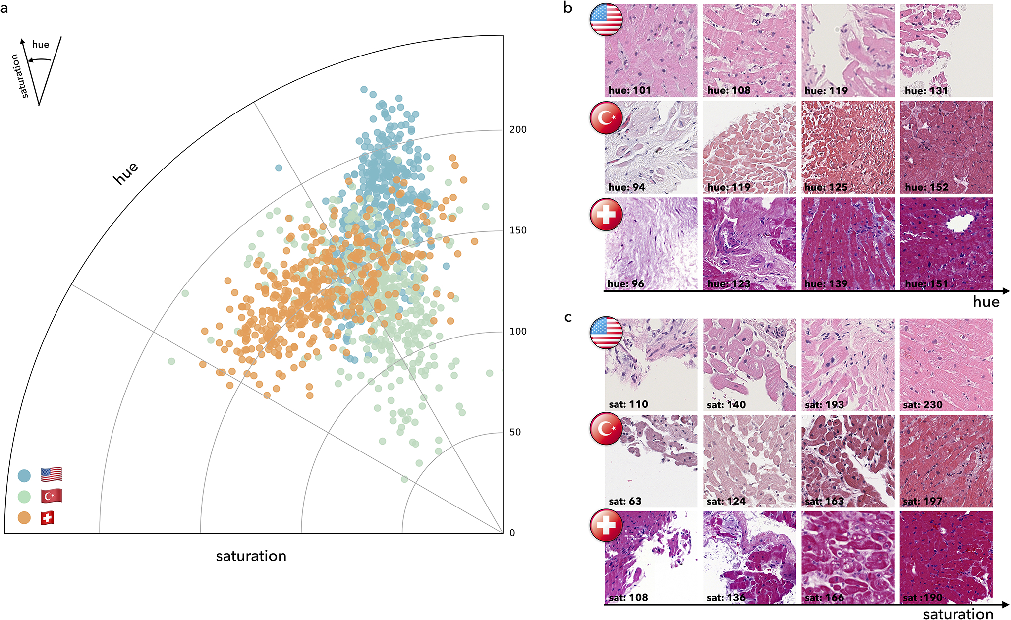
Visualization of color distribution among the three cohorts. a. Polar scatter plot depicts the differences in the train (US) and test (US, Turkish, Swiss) cohorts, each acquired with different scanners and staining protocols. The angle represents the color (i.e. hue) and the polar axis corresponds to the saturation. Each point represents average hue and saturation of an image patch selected from each cohort. To construct the figure, 100 WSIs were randomly selected from each cohort. For each selected slide, 4 patches of size 1024×1024 at ×10 magnification were randomly selected from the segmented tissue regions. A hue–saturation–density color transform is taken to correct for the logarithmic relationship between light intensity and stain amount. The Swiss cohort demonstrates a large variation in both hue and saturation whereas the US and Turkish cohorts have a relatively uniform saturation but variable hue. Examples of patches with diverse hue and saturation from each cohort are shown in subplots b. and c.

Extended Data Figure 2:

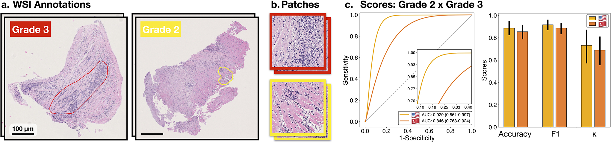
Classification of high-grade cellular rejections. A supervised, patch-level classifier is trained to refine the detected high-grade (2 R+ 3 R) cellular rejections into grades 2 and 3. A subplot a. shows manual annotations of the predictive region for each grade as outlined by pathologist. b. Patches extracted from the respective annotation regions serve as input for the binary classifier. Subplot c. shows the model performance at patches extracted from the US (m = 290 patches) and Turkish (m = 131 patches) cohort. Reported are ROC curves with 95% confidence intervals (CIs). The bar plots represent the model accuracy, F1-score, and Cohen’s κ for each cohort. Error bars indicate the 95% CIs while the center is always the computed value of each classification performance metric (specified by its respective axis labels). The slide-level performance is reported in Supplemental Table 6. The Swiss cohort was excluded from the analysis due to the absence of grade 3 rejections.

Extended Data Figure 3:

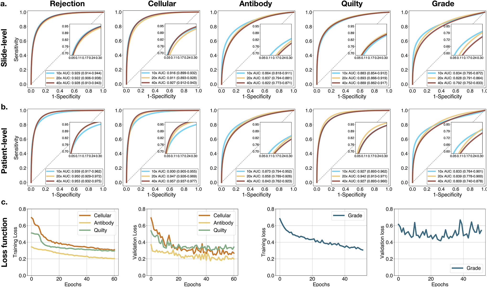
Model performance at various magnifications. Model performance at different magnifications scales at a. slide-level and b. patient-level. Reported are AUC-ROC curves with 95% CI for 40×, 20× and 10× computed for the US test set (n = 995 WSIs, N = 336 patients). For the rejection detection tasks, the model typically performs better at higher magnification, while the grade predictions benefit from the increased context presented at lower magnifications. To account for the information from different scales, the detection of rejections and Quilty-B lesions is performed from the fusion of the model predictions from all available scales. In comparison, the rejection grade is determined from 10X magnification. c. Model performance during training and validation. Shown is cross-entropy loss for the multi-task model assessing the biopsy state and for the single-task model estimating the rejection grade. Reported is slide-level performance at 40× for the multi-task model, while the grading scores are measured at 10X magnification. The model with the lowest validation loss encountered during the training is used as the final model.

Extended Data Figure 4:

Performance of the CRANE model at slide-level. The CRANE model was evaluated on the test set from the US (n = 995 WSIs, N = 336 patients) and two independent external cohorts from Turkey (n = 1,717, N = 585), and Switzerland (n = 123, N = 123). a. Receiver operating characteristic (ROC) curves for the multi-task classification of EMB and grading at the slide-level. The area under the ROC curve (AUC) scores are reported together with the 95% CIs. b. The bar plots reflect the model accuracy for each task. Error bars (marked by the black lines) indicate 95% CIs while the center is always the computed value for each cohort (specified by the respective axis labels). The results suggest the ability of the CRANE model to generalize across diverse populations, and different scanners and staining protocols, without any domain-specific adaptations. Clinical deployment might benefit from the model’s fine-tuning with the local data and scanners.

Extended Data Figure 5:

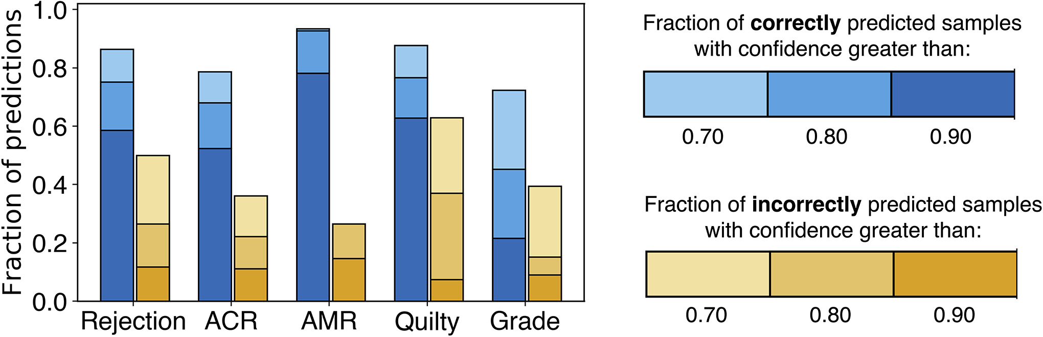
Confidence of model’s predictions. The model robustness can be measured through the confidence of the predictions. The models that suffer from overfitting usually reach high performance on the training dataset by memorizing the specifics of the training data rather than learning the task at hand. As a consequence, such models result in incorrect but highly confident predictions during the deployment. The bar plots show the fraction of model predictions achieved with high confidence, for both correctly (blue) and incorrectly (yellow) estimated patient cases. The fraction of highly confident correctly predicted samples is consistently higher than the fraction of confident incorrect predictions across all the tasks. These results indicate the robustness of the model predictions for all tasks.

Extended Data Figure 6:

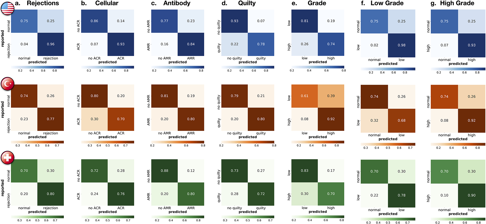
Patient-level performance for all prediction tasks. Reported are confusion matrices for a. rejection detection (including both ACR and AMR), detection of b. ACRs, c. AMRs, d. Quilty-B lesions, and e. discrimination between low (grade 1) and high (grade 2 + 3) rejections. To assess the model’s ability to detect rejections of different grades, subplots f. shows the distinction between normal cases and low-grade rejections, while g. reports distinction between normal cases and high-grade rejections. In both external cohorts, the model reached higher performance for detecting the more clinically relevant high-grade rejections, whereas in the internal cohort the performance is comparable for both low and high-grade cases. The rows of the confusion matrices show the model predictions and the columns represent the diagnosis reported in the patient’s records. The prediction cut-off for each task was computed from the validation set. For the clinical deployment, the cut-off can be modified and fine-tuned with the local data to meet the desirable false-negative rate. The performance is demonstrated on the US hold-out test set (N = 336 patients with 155 normal cases,181 rejections, 161 ACRs, 31 AMRs, 65 Quilty-B lesions, 113 low-grade, and 68 high-grade), Turkey (585 patients with 308 normal cases, 277 rejections, 271 ACRs, 16 AMRs, 74 Quilty-B lesions, 166 low-grade, and 111 high-grade) and Swiss (N = 123 patients with 54 normal cases, 69 rejections, 66 ACRs, 10 AMRs,18 Quilty-B lesions, 59 low-grade and 10 high-grade). Details on each cohort are reported in Supplemental Table 1.

Extended Data Figure 7:

Analysis of case with concurrent cellular, antibody-mediated rejection, and Quilty-B lesions. a-b. The selected biopsy region and the corresponding H&E stained WSI. Attention heatmaps are computed for each task (c,d,e) and the grade (f). For the cellular task (c.), the high-attention regions correctly identified diffuse, multi-focal interstitial inflammatory infiltrate, predominantly comprised of lymphocytes, and associated myocyte injury. For the antibody heatmap (d.), the high-attention regions identified interstitial edema, endothelial swelling, and mild inflammation, consisting of lymphocytes and macrophages. For the Quilty-B heatmap (e.), the high-attention regions highlighted a focal, dense collection of lymphocytes within the endocardium, with mild crush artifact. For the grade (f.), the high-attention regions identified areas with diffuse, interstitial lymphocytic infiltrate with associated myocyte injury, corresponding to high grade cellular rejection. The high-attention regions for both types of rejection and Quilty-B lesions appear similar at the slide level at low power magnification, since all three tasks assign high-attention to regions with atypical myocardial tissue. However, at higher magnification, the highest attention in each task comes from regions with the task-specific morphology. The image patches with the highest attention scores from each task are shown in the last column. This example also illustrates the potential of CRANE to discriminate between ACR and similarly appearing Quilty-B lesions.

Extended Data Figure 8:

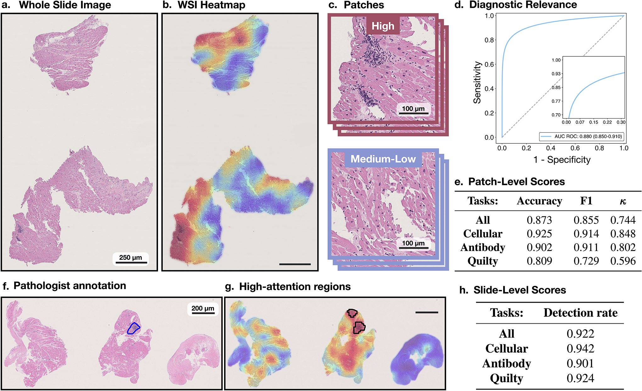
Quantitative assessment of attention heatmaps’ interpretability. While the attention scores provide only relative importance of each biopsy regions for the model predictions, we attempted to quantify their relevance for diagnostic interpretability at patch- and slide-level. From the internal test set, we randomly selected 30 slides from each diagnosis and computed the attention heatmaps for each task (a-b,f-g).For the patch-level assessment, we selected 3 non-overlapping patches from the highest attention region in each slide. Since the regions with the lowest attention scores often include just a small fraction of tissue, we randomly selected 3 non-overlapping patches from the regions with medium-to-low attentions (i.e. attention scores<0.5). We randomly remove 5% of the patches to prevent pathologist from providing an equal amount of diagnoses, resulting in a total of 513 patches. A pathologist evaluated each patch as relevant or non-relevant for the given diagnosis. The pathologist’s scores are compared against the model predictions of diagnostically relevant (high-attention) vs non-relevant (medium-to-low attention) patches. The subplot shows AUC-ROC scores across all patches, using the normalized attention scores as the probability estimates. The accuracy, F1-score, and Cohen’s κ, computed for all patches and for the specific diagnoses, are reported in e. These results suggest a high agreement between the model and pathologist’s interpretation of diagnostically relevant regions. For the slide-level assessment, we compare concordance in the predictive regions used by the model and pathologists. A pathologist annotated in each slide the most relevant biopsy region(s) for the given diagnosis f. The regions with the top 10% highest attentions scores in each slide are used to determine the most relevant regions used by the model g. These are compared against the pathologist’s annotations. The detection rate for all slides, and the individual diagnosis, are reported in h. Although the model did not use any pixel-level annotations during training these results imply relatively high concordance in the predictive regions used by the model and pathologist. It should be noted that the attention heatmaps are always normalized and not absolute, hence, the highest attended region is considered for the analysis similar to 17.

Extended Data Figure 9:

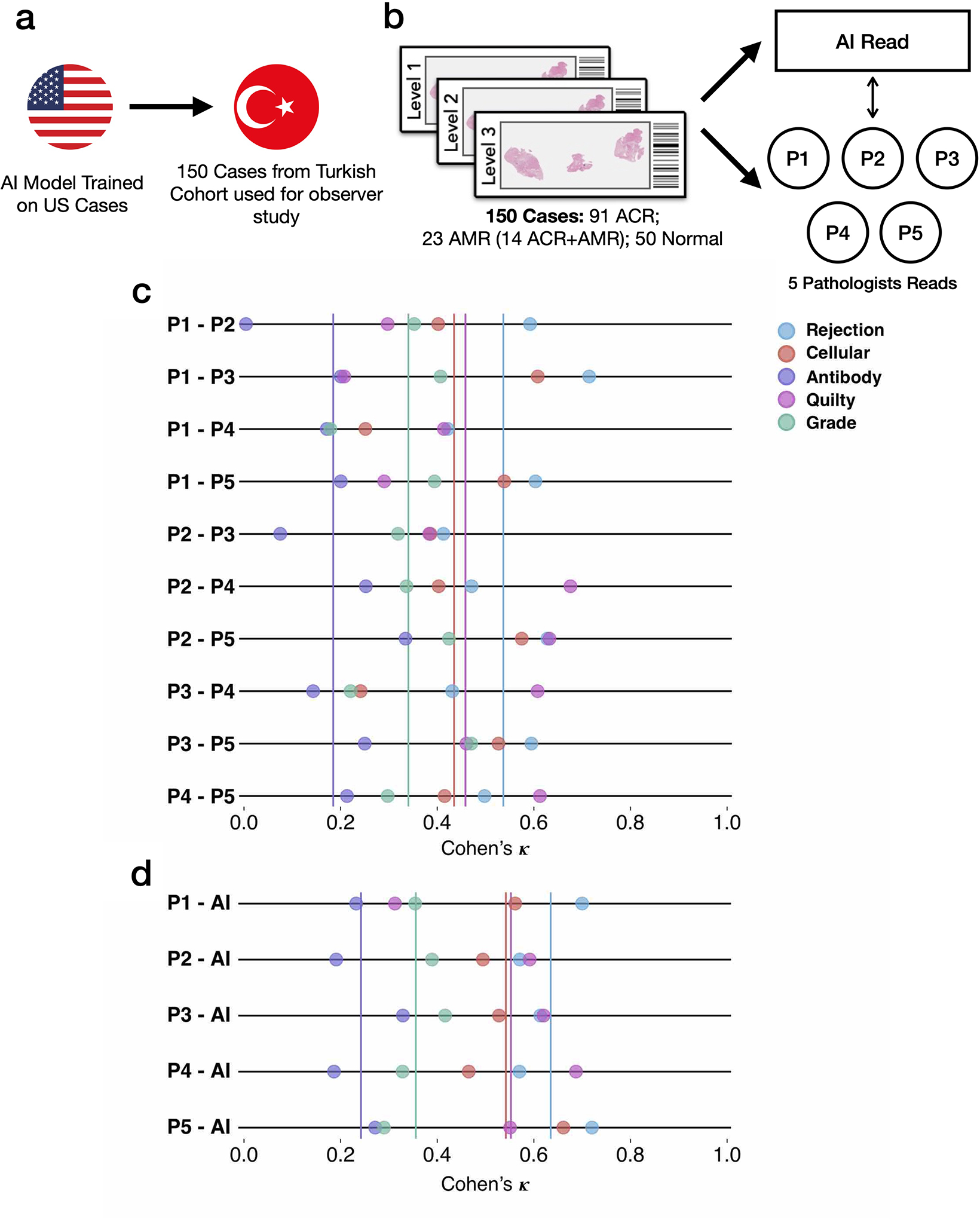
Inter-observer variability analysis. The design of the reader study is depicted in a-b. The subplot c. shows the agreement between each pair of pathologists, while the agreement between the AI model and each pathologist is shown in d. The average agreement for each task is plotted as a vertical solid line. The analysis was performed on a random subset of 150 cases randomly selected from the Turkey test cohort: 91 ACR, 23 AMR cases (including 14 concurrent ACR and AMR cases) and 50 normal biopsies. The AI model was trained on the US cohort. For evaluation purposes, the pathologists assessed each case using the H&E slides only. It should be noted that the assessment presented here is based on Cohen’s κ and is not the absolute agreement. Cohen’s κ is a metric which runs between −1 and 1 and takes into account agreement by chance.

Extended Data Figure 10:

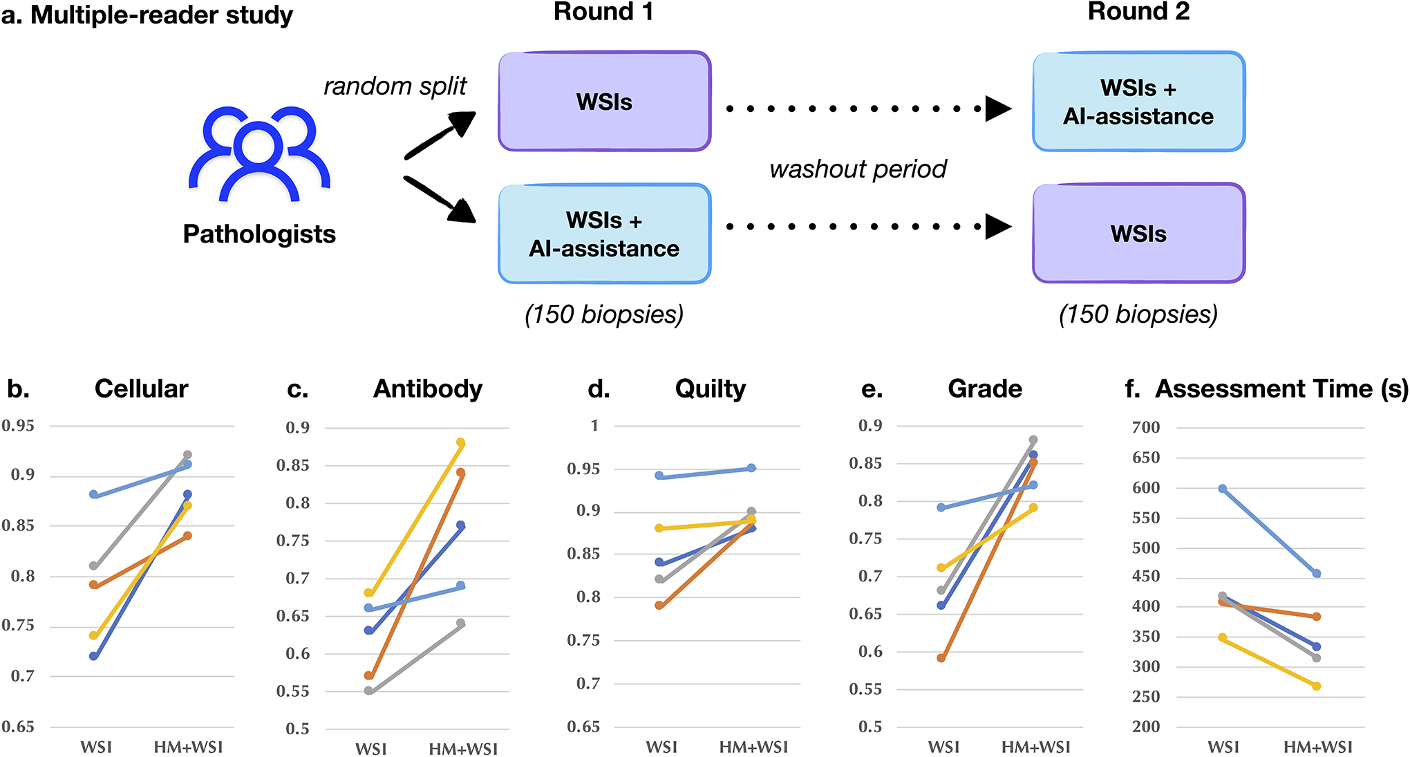
AI-assisted biopsy assessment. An independent reader study was conducted to assess the potential of the CRANE to serve as an assisting diagnostic tool. Subplot a. illustrates the study design. A panel of five cardiac pathologists from an independent center was asked to assess 150 EMBs randomly selected from the Turkey cohort, the same set of slides as used for the assessment of interobserver variability presented in Extended Data Fig. 9. The pathologists were randomly split into two groups. In the first round, the readers from the first group used WSIs only, while the readers from the second group also received assistance from the CRANE in the form of attention heatmaps (HMs) plotted on the top of H&E slides. Following a washout period, the pathologists repeated the task. In the second round, the readers from the first group received WSIs and AI assistance, while the second group used WSIs only. Subplots b-e. report accuracy and assessment time (f.) of the readers without and with AI assistance marked as (WSI) and (HM + WSI), respectively. The ground truth labels were constructed based on the pathologists’ consensus from the reader-study presented in Extended Data Fig. 9. The ability of the CRANE to mark diagnostically relevant regions has increased the accuracy of manual biopsy assessment for all tasks and all readers, as well as reduce the assessment time. These results support the feasibility of CRANE in reducing the interobserver variability and increasing the efficiency of manual biopsy reads.

Data Availability

Please email all requests for academic use of raw and processed data to the corresponding author. Restrictions apply to the availability of the in-house and external data, which were used with institutional permission for the current study, and are thus not publicly available. All requests will be promptly evaluated based on institutional and departmental policies to determine whether the data requested is subject to intellectual property or patient privacy obligations. Data can only be shared for non-commercial academic purposes and will require a data user agreement. A subset of whole slide images used in the study can be accessed through our interactive demo available at http://crane.mahmoodlab.org. ImageNet data is available at https://image-net.org/

References

- [1].Ziaeian Boback and Fonarow Gregg C. “Epidemiology and aetiology of heart failure”. In: Nature Reviews Cardiology 13.6 (2016), pp. 368–378. [DOI] [PMC free article] [PubMed] [Google Scholar]
- [2].Benjamin Emelia J et al. “Forecasting the future of cardiovascular disease in the United States: a policy statement from the American Heart Association.” In: Circulation 137.12 (2018), e67–e492. [DOI] [PubMed] [Google Scholar]
- [3].Badoe Nina and Shah Palak. “History of Heart Transplant”. In: Contemporary Heart Transplantation (2020), pp. 3–12. [Google Scholar]
- [4].Orrego Carlos M et al. “Usefulness of routine surveillance endomyocardial biopsy 6 months after heart transplantation”. In: The Journal of heart and lung transplantation 31.8 (2012), pp. 845–849. [DOI] [PubMed] [Google Scholar]
- [5].Lund Lars H et al. “The Registry of the International Society for Heart and Lung Transplantation: thirtyfourth adult heart transplantation report—2017; focus theme: allograft ischemic time”. In: The Journal of Heart and Lung Transplantation 36.10 (2017), pp. 1037–1046. [DOI] [PubMed] [Google Scholar]
- [6].Colvin-Adams Monica and Agnihotri Adheesh. “Cardiac allograft vasculopathy: current knowledge and future direction”. In: Clinical transplantation 25.2 (2011), pp. 175–184. [DOI] [PubMed] [Google Scholar]
- [7].Kfoury Abdallah G et al. “Cardiovascular mortality among heart transplant recipients with asymptomatic antibody-mediated or stable mixed cellular and antibody-mediated rejection”. In: The Journal of heart and lung transplantation 28.8 (2009), pp. 781–784. [DOI] [PubMed] [Google Scholar]
- [8].Costanzo Maria Rosa et al. The International Society of Heart and Lung Transplantation Guidelines for the care of heart transplant recipients. 2010. [DOI] [PubMed]
- [9].Kobashigawa Jon A. The search for a gold standard to detect rejection in heart transplant patients: are we there yet? 2017. [DOI] [PubMed]
- [10].Angelini Annalisa et al. “A web-based pilot study of inter-pathologist reproducibility using the ISHLT 2004 working formulation for biopsy diagnosis of cardiac allograft rejection: the European experience”. In: The Journal of heart and lung transplantation 30.11 (2011), pp. 1214–1220. [DOI] [PubMed] [Google Scholar]
- [11].Crespo-Leiro Maria G et al. “Concordance among pathologists in the second cardiac allograft rejection gene expression observational study (CARGO II)”. In: Transplantation 94.11 (2012), pp. 1172–1177. [DOI] [PubMed] [Google Scholar]
- [12].Esteva Andre et al. “Dermatologist-level classification of skin cancer with deep neural networks”. In: nature 542.7639 (2017), pp. 115–118. [DOI] [PMC free article] [PubMed] [Google Scholar]
- [13].Bejnordi Babak Ehteshami et al. “Diagnostic assessment of deep learning algorithms for detection of lymph node metastases in women with breast cancer”. In: Jama 318.22 (2017), pp. 2199–2210. [DOI] [PMC free article] [PubMed] [Google Scholar]
- [14].Ouyang David et al. “Video-based AI for beat-to-beat assessment of cardiac function”. In: Nature 580.7802 (2020), pp. 252–256. [DOI] [PMC free article] [PubMed] [Google Scholar]
- [15].Cameron Chen Po-Hsuan et al. “An augmented reality microscope with real-time artificial intelligence integration for cancer diagnosis”. In: Nature medicine 25.9 (2019), pp. 1453–1457. [DOI] [PubMed] [Google Scholar]
- [16].McKinney Scott Mayer et al. “International evaluation of an AI system for breast cancer screening”. In: Nature 577.7788 (2020), pp. 89–94. [DOI] [PubMed] [Google Scholar]
- [17].Lu Ming Y et al. “Data-efficient and weakly supervised computational pathology on whole-slide images”. In: Nature Biomedical Engineering (2021), pp. 1–16. [DOI] [PMC free article] [PubMed] [Google Scholar]
- [18].Campanella Gabriele et al. “Clinical-grade computational pathology using weakly supervised deep learning on whole slide images”. In: Nature medicine 25.8 (2019), pp. 1301–1309. [DOI] [PMC free article] [PubMed] [Google Scholar]
- [19].Bulten Wouter et al. “Automated deep-learning system for Gleason grading of prostate cancer using biopsies: a diagnostic study”. In: The Lancet Oncology 21.2 (2020), pp. 233–241. [DOI] [PubMed] [Google Scholar]
- [20].Chen Richard J et al. “Pathomic fusion: an integrated framework for fusing histopathology and genomic features for cancer diagnosis and prognosis”. In: IEEE Transactions on Medical Imaging (2020). [DOI] [PMC free article] [PubMed] [Google Scholar]
- [21].Mahmood Faisal et al. “Deep adversarial training for multi-organ nuclei segmentation in histopathology images”. In: IEEE transactions on medical imaging (2019). [DOI] [PMC free article] [PubMed] [Google Scholar]
- [22].Fu Yu et al. “Pan-cancer computational histopathology reveals mutations, tumor composition and prognosis”. In: Nature Cancer 1.8 (2020), pp. 800–810. [DOI] [PubMed] [Google Scholar]
- [23].Kather Jakob Nikolas et al. “Pan-cancer image-based detection of clinically actionable genetic alterations”. In: Nature Cancer 1.8 (2020), pp. 789–799. [DOI] [PMC free article] [PubMed] [Google Scholar]
- [24].Lu Ming Y et al. “AI-based pathology predicts origins for cancers of unknown primary”. In: Nature (2021), pp. 1–5. [DOI] [PubMed] [Google Scholar]
- [25].Peyster Eliot G et al. “An automated computational image analysis pipeline for histological grading of cardiac allograft rejection”. In: European Heart Journal 42.24 (2021), pp. 2356–2369. [DOI] [PMC free article] [PubMed] [Google Scholar]
- [26].Tong Li et al. “Predicting heart rejection using histopathological whole-slide imaging and deep neural network with dropout”. In: 2017 IEEE EMBS International Conference on Biomedical & Health Informatics (BHI). IEEE. 2017, pp. 1–4. [DOI] [PMC free article] [PubMed] [Google Scholar]
- [27].Nirschl Jeffrey J et al. “A deep-learning classifier identifies patients with clinical heart failure using whole-slide images of H&E tissue”. In: PloS one 13.4 (2018). [DOI] [PMC free article] [PubMed] [Google Scholar]
- [28].Peyster Eliot G, Madabhushi Anant, and Margulies Kenneth B. “Advanced morphologic analysis for diagnosing allograft rejection: the case of cardiac transplant rejection”. In: Transplantation 102.8 (2018), p. 1230. [DOI] [PMC free article] [PubMed] [Google Scholar]
- [29].Tellez David et al. “Neural image compression for gigapixel histopathology image analysis”. In: IEEE transactions on pattern analysis and machine intelligence (2019). [DOI] [PubMed] [Google Scholar]
- [30].Chen Chi-Long et al. “An annotation-free whole-slide training approach to pathological classification of lung cancer types using deep learning”. In: Nature communications 12.1 (2021), pp. 1–13. [DOI] [PMC free article] [PubMed] [Google Scholar]
- [31].Mun Yechan et al. “Yet Another Automated Gleason Grading System (YAAGGS) by weakly supervised deep learning”. In: npj Digital Medicine 4.1 (2021), pp. 1–9. [DOI] [PMC free article] [PubMed] [Google Scholar]
- [32].Wulczyn Ellery et al. “Deep learning-based survival prediction for multiple cancer types using histopathology images”. In: PLoS One 15.6 (2020), e0233678. [DOI] [PMC free article] [PubMed] [Google Scholar]
- [33].Kanavati Fahdi et al. “Weakly-supervised learning for lung carcinoma classification using deep learning”. In: Scientific reports 10.1 (2020), pp. 1–11. [DOI] [PMC free article] [PubMed] [Google Scholar]
- [34].Schmauch Benoit et al. “A deep learning model to predict RNA-Seq expression of tumours from whole slide images”. In: Nature communications 11.1 (2020), pp. 1–15. [DOI] [PMC free article] [PubMed] [Google Scholar]
- [35].Sellaro Tiffany L et al. “Relationship between magnification and resolution in digital pathology systems”. In: Journal of pathology informatics 4 (2013). [DOI] [PMC free article] [PubMed] [Google Scholar]
- [36].Ilse Maximilian, Tomczak Jakub, and Welling Max. “Attention-based Deep Multiple Instance Learning”. In: International Conference on Machine Learning. 2018, pp. 2132–2141. [Google Scholar]
- [37].Halloran Philip F et al. “Exploring the cardiac response to injury in heart transplant biopsies”. In: JCI insight 3.20 (2018). [DOI] [PMC free article] [PubMed] [Google Scholar]
- [38].Coudray Nicolas et al. “Classification and mutation prediction from non–small cell lung cancer histopathology images using deep learning”. In: Nature medicine 24.10 (2018), pp. 1559–1567. [DOI] [PMC free article] [PubMed] [Google Scholar]
- [39].Karimi Davood et al. “Deep learning with noisy labels: Exploring techniques and remedies in medical image analysis”. In: Medical Image Analysis 65 (2020), p. 101759. [DOI] [PMC free article] [PubMed] [Google Scholar]
- [40].Mitani Akinori, Hammel Naama, and Liu Yun. “Retinal detection of kidney disease and diabetes”. In: Nature Biomedical Engineering (2021), pp. 1–3. [DOI] [PubMed] [Google Scholar]
- [41].Biscotti Charles V et al. “Assisted primary screening using the automated ThinPrep Imaging System”. In: American journal of clinical pathology 123.2 (2005), pp. 281–287. [PubMed] [Google Scholar]
- [42].Halloran Philip F et al. “Building a tissue-based molecular diagnostic system in heart transplant rejection: The heart Molecular Microscope Diagnostic (MMDx) System”. In: The Journal of Heart and Lung Transplantation 36.11 (2017), pp. 1192–1200. [DOI] [PubMed] [Google Scholar]
- [43].Duong Van Huyen Jean-Paul et al. “MicroRNAs as non-invasive biomarkers of heart transplant rejection”. In: European heart journal 35.45 (2014), pp. 3194–3202. [DOI] [PubMed] [Google Scholar]
- [44].Giarraputo Alessia et al. “A Changing Paradigm in Heart Transplantation: An Integrative Approach for Invasive and Non-Invasive Allograft Rejection Monitoring”. In: Biomolecules 11.2 (2021), p. 201. [DOI] [PMC free article] [PubMed] [Google Scholar]
- [45].De Vlaminck Iwijn et al. “Circulating cell-free DNA enables noninvasive diagnosis of heart transplant rejection”. In: Science translational medicine 6.241 (2014), 241ra77–241ra77. [DOI] [PMC free article] [PubMed] [Google Scholar]
- [46].Kennel Peter J et al. “Serum exosomal protein profiling for the non-invasive detection of cardiac allograft rejection”. In: The Journal of Heart and Lung Transplantation 37.3 (2018), pp. 409–417. [DOI] [PubMed] [Google Scholar]
- [47].Anglicheau Dany and Suthanthiran Manikkam. “Noninvasive prediction of organ graft rejection and outcome using gene expression patterns”. In: Transplantation 86.2 (2008), p. 192. [DOI] [PMC free article] [PubMed] [Google Scholar]
- [48].Dong Qi, Gong Shaogang, and Zhu Xiatian. “Imbalanced deep learning by minority class incremental rectification”. In: IEEE transactions on pattern analysis and machine intelligence 41.6 (2018), pp. 1367–1381. [DOI] [PubMed] [Google Scholar]
- [49].Tan Mingxing and Le Quoc. “Efficientnet: Rethinking model scaling for convolutional neural networks”. In: International Conference on Machine Learning. PMLR. 2019, pp. 6105–6114. [Google Scholar]
Associated Data
This section collects any data citations, data availability statements, or supplementary materials included in this article.
Supplementary Materials
Data Availability Statement