Abstract
Object detection is one of the predominant and challenging problems in computer vision. Over the decade, with the expeditious evolution of deep learning, researchers have extensively experimented and contributed in the performance enhancement of object detection and related tasks such as object classification, localization, and segmentation using underlying deep models. Broadly, object detectors are classified into two categories viz. two stage and single stage object detectors. Two stage detectors mainly focus on selective region proposals strategy via complex architecture; however, single stage detectors focus on all the spatial region proposals for the possible detection of objects via relatively simpler architecture in one shot. Performance of any object detector is evaluated through detection accuracy and inference time. Generally, the detection accuracy of two stage detectors outperforms single stage object detectors. However, the inference time of single stage detectors is better compared to its counterparts. Moreover, with the advent of YOLO (You Only Look Once) and its architectural successors, the detection accuracy is improving significantly and sometime it is better than two stage detectors. YOLOs are adopted in various applications majorly due to their faster inferences rather than considering detection accuracy. As an example, detection accuracies are 63.4 and 70 for YOLO and Fast-RCNN respectively, however, inference time is around 300 times faster in case of YOLO. In this paper, we present a comprehensive review of single stage object detectors specially YOLOs, regression formulation, their architecture advancements, and performance statistics. Moreover, we summarize the comparative illustration between two stage and single stage object detectors, among different versions of YOLOs, applications based on two stage detectors, and different versions of YOLOs along with the future research directions.
Keywords: Object detection, Convolutional neural networks, YOLO, Deep learning, Computer vision
Introduction
Object detection is an important field in the domain of computer vision. Various machine learning (ML) and deep learning (DL) models are employed for the performance enhancement in the process of object detection and related tasks. In the earlier time, two stage object detectors were quite popular and effective. With the recent development in single stage object detection and underlying algorithms, they have become significantly better in comparison with most of the two stage object detectors. Moreover, with the advent of YOLOs, various applications have utilized YOLOs for object detection and recognition in various context and performed tremendously well in comparison with their counterparts two stage detectors. This motivates us to write a specific review on YOLO and their architectural successors by presenting their design details, optimizations proposed in the successors, tough competition to two stage object detectors, etc. This section presents the brief introduction of deep learning and computer vision, object detection and related terminologies, challenges, stages and their role in the implementation of any object detection algorithm, brief evolution of various object detection algorithms, popular datasets utilized, and the major contributions of the review.
Deep learning and computer vision
Deep Learning (DL) was introduced in the early 2000s after Support vector machines (SVM), Multilayer perceptron (MLP), Artificial Neural Networks (ANN), and other shallower neural networks became popular. Many researchers termed it as a subset of Machine learning (ML) which is considered as a subset of Artificial Intelligence (AI) in turn. During its inception period, deep learning didn’t draw much attention due to scalability and several other influential factors such as demand of huge compute power. After 2006, it has changed its gear and became popular as compared to its contemporary ML algorithms because of two main reasons: (i) Availability of abundance of data for processing and (ii) Availability of high-end computational resources. The success stories of deep learning in various domains includes weather forecasting [80], stock market prediction [53], speech recognition [59], object detection [37], character recognition [83], intrusion detection [32], automatic landslide detection [48], time series prediction [8], text classification [33], gene expression [51], micro-blogs [82], biological data handling [38], unstructured text data mining with fault classification [75], video processing such as caption generation [78], and many more.
Computer vision is a predominant and versatile field in the current era and lots of research is being carried out by various researchers in this field. Computer vision instructs machines to understand, grasp, and analyze a high-level understanding of visual contents. Its subfields include scene or object recognition, object detection, video tracking, object segmentation, pose and motion estimation, scene modeling, and image restoration [49]. In this review, we focus on the object detection and its relevant subfields such as object localization and segmentation, one of the most important and popular tasks of computer vision. The common deep learning models can be utilized for any computer vision task includes Convolution Neural Network (CNN), Deep Belief Networks (DBN), Deep Boltzmann Machines (DBM), Restricted Boltzmann Machines (RBM), and Stacked Autoencoders [71].
Object classification and localization
Image Classification is a task of classifying an image or an object in an image into one of the predefined categories. This problem is generally solved with the help of supervised machine learning or deep learning algorithms wherein the model is trained on a large labelled dataset. Some of the commonly used machine learning models for this task includes ANN, SVM, Decision trees, and KNN [66]. However, on the deep learning side, CNNs and its architectural successors and variants dominate other deep models for classifying images and related works. Apart from well-defined machine learning and deep learning models, one can also witness the usage of other approaches such as Fuzzy logic and Genetic algorithms for the aforementioned tasks [19].
Object Localization is the task of determining position of an object or multiple objects in an image/frame with the help of a rectangular box around an object, commonly known as a bounding box. However, Image segmentation is the process of partitioning an image into multiple segments wherein a segment may contain a complete object or a part of an object. Image segmentation is commonly utilized to locate objects, lines, and curves viz. boundaries of an object or segment in an image. Generally, pixels in a segment possess a set of common characteristics such as intensity, texture, etc. The main motive behind image segmentation is to present the image into a meaningful representation. Moreover, Object detection can be considered as a combination of classification, localization, and segmentation. It is the task of correctly classifying and efficiently localizing single or multiple objects in an image, generally with the help of supervised algorithms given a sufficiently large labelled training set. Figure 1 presents the clear understanding of classification, localization, and segmentation for single and multiple objects in an image in the context of object detection.
Fig. 1.
Classification, Localization, and Segmentation in Single and Multiple Objects image [13]
Challenges in object detection
Applications of object detection have a broad range covering autonomous driving, detecting aerial objects, text detection, surveillance, rescue operations, robotics, facing detection, pedestrian detection, visual search engine, computation of object of interest, brand detection, and many more [1, 58]. The major challenges in the object detection includes; (i) The occupancy of an object in an image has an inherent variation such as objects in an image may occupy majority of the pixels i.e., 70% to 80%, or very few pixels i.e., 10% or even less, (ii) Processing of low-resolution visual contents, (iii) Handling varied sized multiple objects in an image, (iv) Availability of labelled data, and (v) Handling overlapping objects in visual content.
Most of the object detectors based on machine learning and deep learning algorithms fail to address commonly faced challenges, are summarized as follows:
Multi-scale training: Most object detectors are trained for a specific resolution of input. These detectors generally underperform for inputs having different scales or resolutions.
Foreground-Background class imbalance: Imbalance or disproportion among the instances of different categories can majorly affects the model performance.
Detection of relatively smaller objects: All the object detection algorithms will tend to perform well on larger objects if the model is trained on larger objects. However, these models show poor performance on comparatively smaller sized objects.
Necessity of large datasets and computational power: Object detection algorithms in deep learning need larger datasets for computation, labor intensive approaches for annotations, and powerful computational resources for processing [45]. Due to the exponential increase of generated data from various sources, it has become a tedious and labor-intensive task to annotate each and every object in the visual contents [45, 73, 80].
Smaller sized datasets: Though deep learning models outperform traditional machine learning approaches by a great margin, they demonstrate poor performance while evaluating on the datasets with fewer instances.
Inaccurate localization during predictions: Bounding boxes are the approximations of the ground-truth. Generally, background pixels are also included during predictions, this affects the accuracy of the algorithm. Mostly, localization errors are either due to occupancy of background in the predictions and detecting similar objects [45].
Stages in object detection
In supervised machine learning, there are two types of problems; (i) Regression and (ii) Classification. However, image classification is no different from the traditional classification problem. The next task after classifying the object in an image is to localize it, if required. A rectangular box, commonly known as a bounding box is determined around an object with the help of the deep neural networks. This object detection problem generally performs the features extraction followed by the classification and/or localization, known as two-stage object detectors if implemented in two stages. First stage generates Regions of Interest (RoI) using Region Proposal Network (RPN), however, the second stage is responsible for predicting the objects and bounding boxes for the proposed regions. First stage mainly responsible for selecting plausible region proposals by applying various techniques such as negative proposal sampling. The popular models in this category include Region based convolutional neural networks (RCNN), Fast RCNN, and Faster RCNN. Single stage object detectors enjoying the simpler architecture, specially designed for the object detection in single stage by considering all the region proposals. These detectors output the bounding boxes and class specific probabilities for the underlying objects by considering all the spatial sizes of an image in one shot. Though, two stage object detectors perform better in comparison with single stage object detectors as it works on highly probable regions only for the object detection.
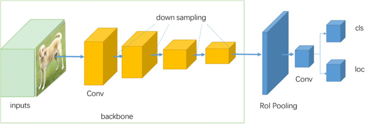
However, with the advent of You Only Look Once (YOLO) and its successors, attempts are being heavily appreciated for solving this task in one shot/stage wherein localization problem is formulated as a regression problem with the help of deep neural networks. YOLO is not the first algorithm that uses Single Shot Detector (SSD) for object detection. There are numerous other algorithms that have been introduced in recent past such as Single Shot Detector (SSD) [43], Deconvolution Single Shot Detector (DSSD) [16], RetinaNet [41], M2Det [86], RefineDet++ [85], are based on single stage object detection. Two stage detectors are complex and powerful and therefore they generally outperform single stage detectors. YOLO can be seen as giving a tough fight to not only two staged detectors but previous single staged detectors also in terms of accuracy and inference time. It is considered as one of the most common choices in production only because of its simple architectural design, low complexity, and easy implementation. Figure 2 shows the generic schematic architecture of single stage object detectors wherein it generates all the bounding boxes along with the class probabilities by considering all the spatial regions in one shot.
Fig. 2.
Generic architecture of single stage object detectors [29]
Evolution of Object Detectors & Related Works
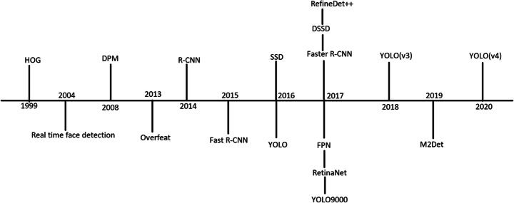
Well known machine learning approaches for object detection include Viola-Jones object detection framework [70] and Histogram of Oriented Gradients (HOG). The former framework was primarily introduced for face detection. The algorithm had three main stages viz. Integral image, Adaboost classifier, and Classifier Cascade. However, HOG was introduced by Robert K. McConnell of Wayland Research Inc. in 1986. Firstly, the image is divided into smaller regions known as cells. A HOG is then calculated for each pixel in the cell and the combination of all the histograms is known as a descriptor. These descriptors are fed as features in traditional classifiers. Dalal and Triggs utilized SVM as a classifier for classifying an object based on these features [34]. Overfeat was another object detector introduced in 2013 that leverages the advantages of spatial convolutional network features. Figure 3 illustrates the year wise evolution of various important algorithms for object detection. Keeping the model’s complexity high and huge resources consumption by two stage object detectors in mind, researchers concentrate on single stage object detectors and in particular YOLO algorithms, shall be covered in detail in the next section.
Fig. 3.
Year wise evolution of object detection algorithms
Deep learning is not only performing well in object detection but in other fields also. Deep learning is offering various models to efficiently handle the healthcare related data. Since the inception of Covid-19 outbreak, different sources such as X-ray, CT, and MRI are being heavily utilized for the possible infection due to virus. The role and applicability of various deep models for the detection of Covid-19 infection are summarized in [4]. Among all the deep learning models, CNN has gained huge popularity in the feature extraction from visual inputs. As an example, CNN based hand recognition system has achieved 100% training and testing accuracy while applying crow search algorithm (CSA) for searching the optimal hyperparameters [18]. A machine learning model is developed for the tomato disease dataset classification wherein PCA based whale optimization is utilized for the efficient features’ selection [17]. The extracted features are then fed into another deep model for further classification of tomato disease. Binary classification of malwares on image datasets using CNN is implemented in [69]. The proposed solution outperforms the state-of-the-arts pretrained CNNs in the course of malware detection and classification using visual inputs.
Popular dataset and characteristics
MicroSoft Common Objects in COntext (MSCOCO) dataset is one of the standards and most popular datasets in computer vision tasks. This dataset was primarily designed for experimenting image/object classification, detection, and instance segmentation tasks using ML/DL based approaches. This dataset comes with fewer categories; however, it comprises more instances in each category. Specifically, it includes 91 different categories of objects like person, dog, train, and other commonly encountered objects. In addition to the large number of instances in each category, it also observes multiple instances with different characteristics per image [40]. Pascal Visual Object Classes (Pascal VOC) [14] is another benchmarking dataset for visual object classification, segmentation, and detection. The dataset community has constantly been contributing every year starting with 4 classes in 2005 to 20 classes in 2007, making it competitive with recent advancements. The various classes of Pascal VOC are presented in Table 1. Approximately, 11,530 images are comprised in the training dataset which contains 27,540 Region of Interests (RoI) and 6929 segmentations.
Table 1.
PASCAL VOC classes [14]
| Vehicles | Household | Animals | Others |
|---|---|---|---|
| Aeroplane | Bottle | Bird | Person |
| Bicycle | Chair | Cat | |
| Boat | Dining Table | Cow | |
| Bus | Potted Plant | Dog | |
| Car | Sofa | Horse | |
| Motorbike | TV/Monitor | Sheep | |
| Train | |||
Over the recent years, the commonly used metric for evaluation in Object detection is Average Precision (AP), can be defined as the average detection precision under various recalls and evaluated in a class-specific manner. In order to compare the performance of all the categories of objects, an average of all the object categories i.e., mean Average Precision (mAP) is used as a final metric for evaluation in the object detection and related fields.
Importance of the review
Most of the reviews and surveys cover the two stage object detection algorithms. To the best of our knowledge, this is the first review that covers the single stage object detection using specially YOLOs. Herein, we present an extensive review on single stage object detection algorithms based on underlying architectures, regression formulation, pros and cons, comparative and incremental approach in this category, popular datasets, results obtained, and future scope. The main contributions of this paper are summarized as follows:
Presenting the challenges and role of stages in the object detection process.
Brief explanation over two stage object detectors along with their applications.
Necessity of single stage object detectors and detailed review of YOLOs in terms of incremental architectural aspects, proposed optimization techniques, significance of loss function, and YOLOs based applications.
Comparative illustration between two stage and single stage object detectors, among different version of YOLOs in term of performance and results along with the future research direction in single stage object detectors.
Organization of the Paper
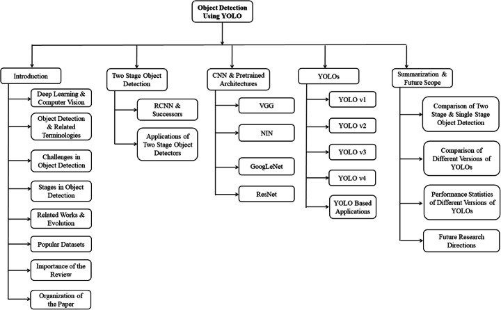
The rest of the paper is organized as follows. Section 2 briefly covers some of the popular two stage object detectors such as RCNN, Fast-RCNN, and Faster-RCNN along with the applications of these two stage object detectors. Section 3 summarizes the architectural aspects of CNN along with several pretrained models such as VGG, Network in Network, ResNet, and GoogleLeNet, utilized in the different versions of YOLOs. Section 4 presents the detailed description of regression formulation, design concepts of YOLO, its architectural successors, and various applications based on different versions of YOLOs. Lastly, we summarize the paper by presenting comparative illustration between two stage and single stage object detector, comparative illustration among different version of YOLOs along with their statistical results and performance. This section also presents the future research directions in object detections at last. However, the detailed flow of the paper is illustrated using Fig. 4.
Fig. 4.
Organization of the Review
Two stage object detection
Recent object detection algorithms can be categorized broadly into two types viz. Two stage object detectors and Single stage object detectors. In the former one, the first stage is responsible for generating Regions of Interest (RoI) using Region Proposal Network (RPN), however, the second stage is responsible for predicting the objects and bounding boxes for the proposed regions. We explore some popular two stage object detectors along with their usage and applicability in various domains in this section.
R-CNN and successors
In the first stage of region proposal, few key algorithms such as Deformable Parts Models (DPM) [15] and OverFeat [61] utilized sliding window technique wherein a fixed-sized window slides through entire image and outputs the region proposals after passing through the classifier. The process is repeated with increasing window size. R-CNN and its successors use selective search algorithm to extract region proposals. R-CNN is a region based convolutional neural network object detection algorithm proposed by Ross Girshick [21]. They divided the solution in three modules: 1) Region proposals are generated using a selective search algorithm, 2) Each region proposal is passed through the architecture having five convolutional layers followed by two dense layers, generating a feature vector of size 4096, and 3) Third module has independent linear classifiers pre-trained for each class. A feature vector is passed through these linear classifiers obtaining class specific scores. Lastly, non-max suppression is applied on all the scores to obtain the best fit.
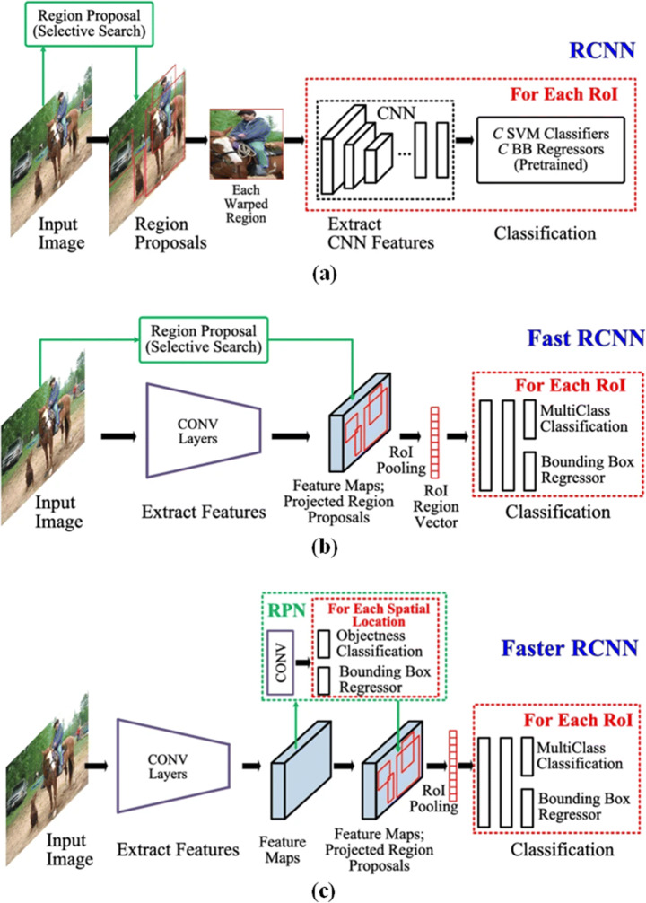
Fast R-CNN [20] achieves a significant improvement in the model training time and inference time. Moreover, it also observes an increase in the performance matrix of the object detection i.e., mAP. Single stage object detection is realized with the help of multi-task loss function wherein all the networks’ layers can be updated in the model training without any specific requirement of disk storage for caching the features. It takes the entire image and object proposals as an input. The entire image is fed into the network to generate a feature map from which features vector is generated by RoI for each object proposal. Each feature vector is fed into a fully connected layer with a SoftMax activation function to output class probabilities and a bounding box offset. Faster R-CNN [57] is a successor of Fast R-CNN and it was released in early 2016. It has 2 modules; 1) First is a CNN i.e., Region proposal network which is responsible for generating region proposals. It takes a single image as an input and outputs the bounding boxes and object confidence scores, 2) During training, RPN is trained on ImageNet then regional proposals are used for detection and training separately, finally Fast R-CNN is fine-tuned with unique dense layers. In the experimentational setup for object detection on Pascal VOC 2007, Fast-RCNN and Faster-RCNN are 25 and 250 times faster respectively compared to traditional RCNN with almost similar mAP of around 66. Figure 5 illustrates these two stage object detectors and an incremental improvement in the architecture.
Fig. 5.
Two stage object detectors (a) RCNN (b) Fast-RCNN (c) Faster-RCNN [44]
Other than the aforementioned two stage object detectors, several other instances are also quite popular. As the scope of the review is limited to single stage object detectors specially YOLOs, we are not including other two stage object detectors in detail here. However, Feature Pyramid Network (FPN) [42] is one of the important two stage object detectors, tried to overcome few of the aforementioned challenges successfully by extracting features at multiple scales of an image in the object detection process.
Applications of R-CNN and successors
There are numerous applications wherein two-phase object detectors are employed and achieved benchmarking results. We shall not cover the entire corpus; however, we list some of them in Table 2, to demonstrate the broad spectrum of two stage object detectors. RCNN and its successors have been frequently used for tracking the objects from a drone-mounted camera. Real time object detection and tracking is implemented and benchmarking results are obtained using embedded hardware such as Jetson TX/AGX Xavier and Intel Neural Compute Stick wherein RCNN is employed on the embedded hardware for object detection [26]. A novel OCR system is developed, named as Rosetta, wherein faster-RCNN is utilized for detecting the text characters from millions of Facebook images, however, fully convolutional CNN is employed for generating the lexicon free transcription of each word [6]. A group of researchers from Google developed an application using computer vision, machine learning, and Google’s Knowledge Graph called as Google Lens [22] wherein a region proposal network (RPN) is utilized to detect the character level bounding boxes for text recognition.
Table 2.
Applications of Two stage object detectors
| Ref. | Application | Model Based on | Key characteristics | Performance Metrics |
|---|---|---|---|---|
| [26] | Object detection using drone mounted camera | RCNN |
• Embedded Hardware: Jetson TX/AGX Xavier and Intel Neural Compute Stick • Realtime object Detection |
• 0.9 fps |
| [6] | Rosetta | Faster-RCNN |
• OCR system • Faster-RCNN for character recognition from Facebook images • Lexicon free transcription generation |
• 8.2% relative improvement for 1000 RPN Post NMS Top N |
| [62] | Object detection and recognition | Faster-RCNN |
• Utilization of faster RCNN for increasing model precision and decreasing detection loss • Usage of saliency detection, proposal generation and bounding box regression by faster-RCNN |
• 74.6 mAP |
| [63] | Detection of defected paper tube in silk industry | Faster-RCNN |
• Efficient detection of the internal joints in the paper tube • Better performance in varying lighting conditions |
• 98% detection accuracy |
| [74] | Person recognition | Semi-supervised faster RCNN |
• Distant video surveillance with challenges as low resolution, heat haze presence, and shaking cameras • Person recognition and carrying load monitoring via high end cameras • Faster RCNN based on ResNet50 and GoogLeNet Transfer learning |
• False positive rate-15.93%, True positive rate-59.16%, False negative rate-40.84% for a threshold of 0.0001 |
| [24] | Traffic sign detection | Faster-RCNN |
• Traffic lights and distant road signs detection in surveillance video or driving reorder videos • Challenge: these objects cover only 5% of the imagen |
• An improvement of around 12% in the mAP |
| [72] | Building area recognition | Faster-RCNN |
• A combination of Faster-RCNN and ZF convolutional neural network • Construction and annotation of the dataset of building images |
• Faster detection of building area |
| [77] | Clothing image recognition | RCNN |
• Modified selective search to extract region proposal • Inception-ResNet to better represent image • Soft-NMS to correct the boundaries of region box |
• 73.59% Precision • 83.84% Recall |
By looking at the performance metrics shown in Table 2, we can observe the two objective functions viz. Reduction in the processing or inference time and Improvements in the performance metrics. As per the characteristics of the fast or faster CNN, reduced inference time is observed by applying these architectures in comparison with its shallow counterpart RCNN. Frames per second (fps) is one of the major metrics on which processing or inference speed is evaluated.
Convolutional neural networks and Pretrained models
Traditional machine learning algorithms completely rely on the handcrafted features extraction followed by feature selection for performing any prediction or classification tasks. Usually, these algorithms spend a huge amount of time in choosing the best method for feature extraction. In order to overcome these drawbacks, researchers, industrialists, and academicians are actively working in deep learning. Commonly used deep learning techniques/models include deep neural networks, Convolutional Neural Networks (CNN), Recurrent Neural Networks (RNN) and its architectural variants such as Long Short-Term Memory (LSTM) and Gated Recurrent Unit (GRU), Generative Adversarial Network (GAN), and different types of autoencoders. Due to scaling inefficacy in deep neural networks, CNN is widely adopted to capture the spatial and contextual information with fewer parameters. While dealing with high-dimensional inputs such as images, it is almost impractical to connect all neurons in a given layer to all neurons in the previous layer. Instead, we connect each neuron to only a part of the previous layer.
Coming to the architectural design of CNNs, convolutional, pooling, and Rectified Linear Unit (ReLU) collectively act as a basic transformation unit converting an input volume to an output volume. The spatial extent in the convolution operation is a hyperparameter known as a receptive-field or filter-size. Filter-size that convolves over the input plays an important role in extracting useful features information. Other hyperparameters such as depth, stride, and zero-padding decide the size of the output volume [3]. Similar to the regular neural networks, a dot product is performed between the weights (w) and the spatial input (x) and any non-linear activation function (f) is applied after adding the bias term (b). The convolution operation for textual and visual input can be expressed using Eqs. 1 and 2 respectively.
| 1 |
| 2 |
where is the output of the ithneuron in layer l. d is the filter-size in textual input and d1, d2 are the filter-width and filter-height respectively in visual input.
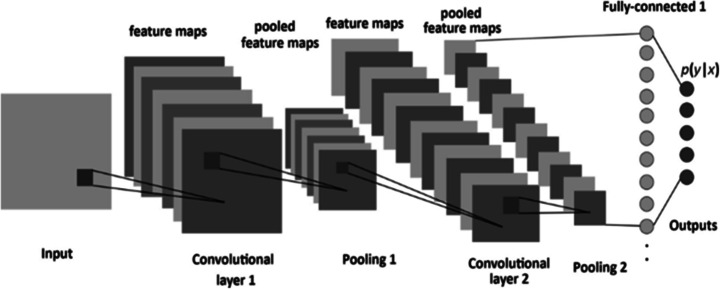
Pooling is generally applied to an output of the conv-layer and this layer performs a down sampling along the spatial dimensions and is useful in extracting the dominating features. There are several types of pooling such as max-pooling, average-pooling, and sum-pooling [68], and each is chosen depending on the application requirements. As an example, features such as negation, whether it is in a textual or visual segment, must have the highest score in the convolution operation so that it can dominate other scores in a max-pooling operation. Max pooling operation for a 1-D input can be expressed using Eq. 3. It can be extended similarly for higher dimensions also. Other pooling can also be computed in a similar fashion. Generally, conv-layer and fully connected layer have ReLU as an activation function. ReLU is a simple non-linear activation function expressed using Eq. 4. The general form of a CNN model can be represented as several consecutive convolutional layers followed by an optional pooling layer, shown using Eq. 5 and presented in Fig. 6. This architecture is stacked several times until the important features are captured completely within an acceptable spatial limit. These convolutional layers are followed by several fully connected layers and then SoftMax is applied for probability estimation. Figure 7 shows the schematic representation of the three fundamental layers used in CNN i.e., convolution, max-pool, and ReLU activation.
Fig. 6.
Generic architecture of Convolutional neural networks [2]
Fig. 7.
Convolutional Neural Network Layered Operations (http://cs231n.github.io/convolutional-networks/). a Conv-layer b Max-pooling layer c ReLU activation
| 3 |
| 4 |
| 5 |
The parameters play a vital role in the CNN architecture, as model complexity is defined by the number of parameters. Several layers such as conv-layer and fully-connected layer have parameters whereas pooling and ReLU may not have parameters. The performance of a structured model after deployment is mostly dominated by the model complexity [10]. Lighter the model, faster the inferences and vice versa, generating a trade-off between the efficacy and performance matrix of a deployed structured model on tensor processing unit (TPU). Researchers proposed the powerful CNN based architectures in an incremental fashion for dealing with image classification, object detection, and image segmentation. There is no specific reason behind designing these architectures in a specific way. Some of the popular architectures used in designing YOLO and its successors are as follows.
VGG
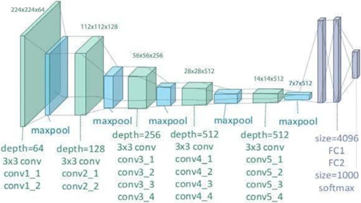
In 2015, K. Simonyan and A. Zisserman developed various architectural innovations to older CNN architectures. The improvised architecture is known as VGG, achieved a top-5 accuracy of 92.7% for an object detection task on the test dataset of ImageNet, a standard dataset containing around 14 million images belonging to 1 k classes. They proposed smart factorization in the convolution operation, specifically, 3 × 3 filters are used throughout the entire architecture to introduce model consistency and to reduce the number of parameters.
Smaller filters result in fewer parameters and are capable of identifying smaller objects more effectively. The authors proposed this architecture in two flavors viz. VGG19 and VGG16, consisting of 19 and 16 layers in the deep neural networks respectively [64]. In several configurations, 1 × 1 convolution is introduced that is considered as depth wise down sampling [60]. With increase in depth of network by series of convolutions, pooling layers and fully connected layers, it has resulted in 138 M parameters approximately [31]. Figure 8 shows the generic schematic of VGG architecture.
Fig. 8.
VGG architecture [50]
Network in network
Min Lin and his contributors didn’t follow the traditional approaches for extracting the features/information. Just like convolutional filters slide throughout the image, in the same fashion, a multilayer perceptron convolution (mlpconv) slides pixel-wise through the entire image and extracts the features, as demonstrated in Fig. 9. Here three layers of mlpconv are stacked followed by a Global Average Pooling (GAP) layer [12]. The underlying working of the GAP layer is presented in Fig. 10. If we have an image of dimension (H × W × D) then after applying global average pooling, we get (1 × 1 × D) tensor. It has resulted in a decrease in number of parameters, so as the model complexity [39]. The average of all the pixel values in each channel is the overall result of the GAP operation. This technique also helps in dimensionality reduction. Additionally, SoftMax is used as an activation function in the last layer and (1 × 1) convolution filters are placed in a multilayer perceptron after convolutional layer resulting in dimensionality reduction [23].
Fig. 9.
Network in Network architecture [39]
Fig. 10.
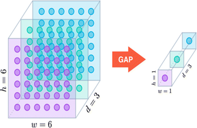
Global Average Pooling [85]
GoogLeNet
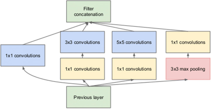
C. Szegedy et al. invoked completely new architecture that introduces multiple filters in the architecture in an elegant manner. An image of any resolution can be fed into this network that was considered as one of the major bottlenecks for earlier models. It has two convolutional layers, two max-pooling layers, and a series of inception modules. According to [65], the inception modules contain three different sizes of filters viz. 1 × 1, 3 × 3, and 5 × 5 for capturing different sized patterns. Before applying any 3 × 3 or 5 × 5 filters, depth-wise down sampling is achieved with the help of 1 × 1 convolution operation. These down sampled output is then introduced to other types of filters. Output of different multiple filters are then cascaded depth-wise as they share the same width and height.
In GoogLeNet, additional max-pooling layers are used in the architecture in addition to the max-pooling of the inception module. This architecture is a deep network with 22 layers but has 12 times less parameters than AlexNet architecture, consisting of 4 million parameters approximately [31]. In order to overcome the problem of vanishing gradients, auxiliary loss is utilized by introducing an intermediate SoftMax classifiers during model training. The loss is back propagated after calculation of loss at each intermediate layer, moreover, computation of total loss is based on all the intermediate losses. It records much better performance than any of the previous architectures on ImageNet dataset. Figure 11 shows the GoogLeNet architecture, however, its building block i.e. inception module is sketched in Fig. 12.
Fig. 11.
GoogLeNet architecture [67]
Fig. 12.
Inception module of the GoogLeNet architecture [65]
ResNet
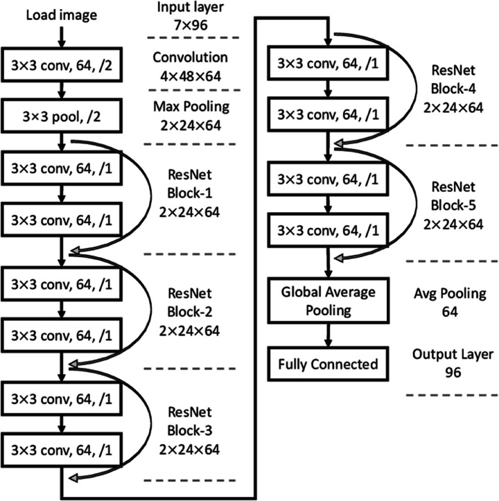
The ResNet architecture is also known as a residual network. The number of layers is increased to 34 which is almost doubled in comparison with VGG19 [64]. The objective here is to improve the model performance by using a deeper network. Unfortunately, the network turned out to be an over parameterized network leading to large training error [25]. Authors introduced the problem of model degradation i.e. model accuracy increases with an increase in the model depth to a certain extent only. Due to the problem of vanishing gradients, the model is unable to update the distant parameters.
Subsequently, the concept of identity mapping is introduced in [11]. A skip or residual connection of length 2 is proposed as shown in Fig. 13. The length of the skip connection can be changed depending upon the application or model requirement. Output of the convolutional layer x + 1 is concatenated with the input of convolutional layer x before providing an input to the convolutional layer x + 2, assuming dimensions are same for concatenation. This also preserves the original information and overcomes the problem of vanishing gradient. However, different techniques may be adopted if these dimensions are mismatched [11]. It is 20 times deeper than AlexNet and 8 times deeper than VGG [23]. In addition, ResNet152 has a total of 25.6 million parameters whereas ResNet110 has 1.7 million parameters [31].
Fig. 13.
ResNet architecture demonstrating the skip connections [11]
Architectural design of YOLOs
In this section, we present the underlying concepts, architectures, incremental approaches across different versions of YOLOs and loss function in the context of YOLO algorithm. Specifically, we elaborate four versions of YOLOs and incremental optimizations adopted in each successor over its predecessor.
Authors of YOLO [56] have reframed the problem of object detection as a regression problem instead of classification problem. A convolutional neural network predicts the bounding boxes as well as class probabilities for all the objects depicted in an image. As this algorithm identifies the objects and their positioning with the help of bounding boxes by looking at the image only once, hence they have named it as You Only Look Once (YOLO). The CNN works impressive on visual input for features’ extraction as low-level features are efficiently propagated from the initial convolutional layers to later convolutional layers in a deep CNN. Herein, the challenge lies in the accurate identification of multiple objects along with their exact positioning present in a single visual input. Parameter sharing and multiple filters are the two important CNN features, capable of handling this object detection problem effectively.
In this object detection process, the image/frame is divided into S × S grid cells, each grid cell predicts B bounding boxes along with their positions and dimensions, probability of an object in the underlying grid, and conditional class probabilities. The fundamental concept behind detection of an object by any grid cell is that the center of an object should lie inside that grid cell. This grid cell is responsible for detecting that particular object with the help of any suitable bounding box. Formally, for a grid, it predicts the following parameters for single bounding box wherein first five parameters are bounding box specific, however, rest are shared across all the bounding boxes for one grid, irrespective of the number of bounding boxes:
| pc | bx | by | bw | bh | p(c1) | p(c2) | ... | ... | ... | ... | ... | ... | ... | p(cn) |
where pc represents probability of containing an object in the grid by the underlying bounding box, (bx, by) indicate the center of the predicted bounding box, (bh, bw) represent predicted dimension of the bounding box, p(ci) means conditional class probability that the object belongs to ith class for the given pc and n is the number of classes/categories. A grid cell predicts (B × 5 + n) values, where B is the number of bounding boxes per grid cell. The output tensor shape would be S × S×(B × 5 + n) as we had divided the image into S × S grid cells. Figure 14 illustrates the final schematic of the output tensor prediction when the input image is divided into 19 × 19 grids as an example and four bounding boxes are predicted per grid wherein class probabilities are shared across all the bounding boxes for a specific grid. Confidence score (cs) is computed for each bounding box per grid by multiplying pc with Intersection over Union (IoU) between the ground-truth and predicted-bounding-box. If object does not exist in the grid cell, confidence score would be zero. In the next step, we compute the class specific score (css) for each bounding box of all the grid cells. This class specific score encodes both the probability of the class appearing in that box and how well the predicted box fits the object.
Fig. 14.
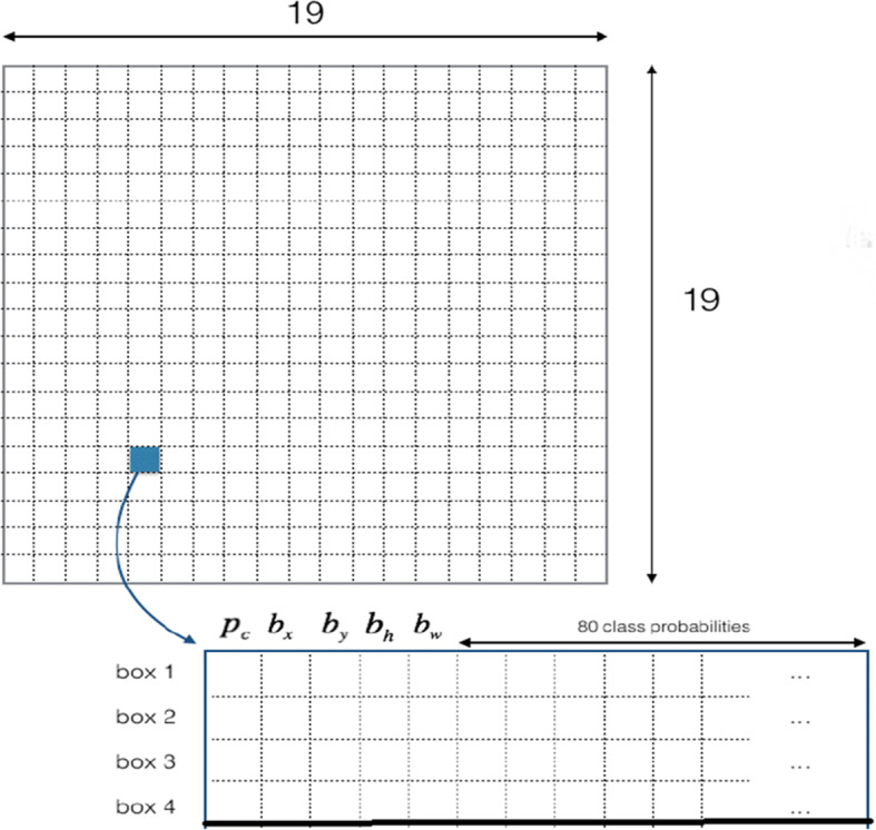
Dividing the image into grid cells and predictions corresponding to one grid cell
Generally, these bounding boxes differ in size, considering different shapes for capturing the different objects, known as anchor boxes. An object in the image should be detected by a bounding box such that the center of the object should reside in that bounding box. However, there may be a possibility of residing centers of multiple objects in the same bounding box. Authors utilized a different term of anchor boxes to represent the bounding boxes corresponding to a single grid cell. Anchor boxes are just a set of several standard bounding boxes, selected after analyzing the dataset and underlying objects in the dataset. These chosen anchor boxes should represent most of the classes/categories by considering different combinations of width and height such as square, vertical or horizontal rectangle, etc. to accommodate the aspect ratio and scale of all the objects present in the dataset.
Adjacent grid cells may also predict the same object i.e., predicting the overlapping bounding boxes for the same object. So, there would be multiple predictions because neighboring grid cells may assume the object center falls inside it. Figure 15a demonstrates the multiple bounding boxes prediction for an object however high and low overlapping between the predicted box and the ground truth is presented in Fig. 15b and Fig. 15c respectively. We need to resolve this issue of detection of the same object by multiple grid cells or by multiple bounding boxes of the same grid cell.
Fig. 15.
Multiple bounding boxes and their overlapping with the ground truth (a) Multiple bounding boxes (b) high overlapping (c) low overlapping
Now, each bounding box of all the grids will be associated with a class specific score, box coordinates, and a classification output category. We will be having a total S2 × B predicted boxes, moreover, boxes will be discarded having a class score lesser than some predefined threshold. Usually, this threshold is taken as 0.5 in most of the object detection algorithms, but it may vary depending upon the dataset and its characteristics. The reason for a low score may be either due to the low probability of containing an object in that grid or low probability of any particular class category that maximizes the class score.
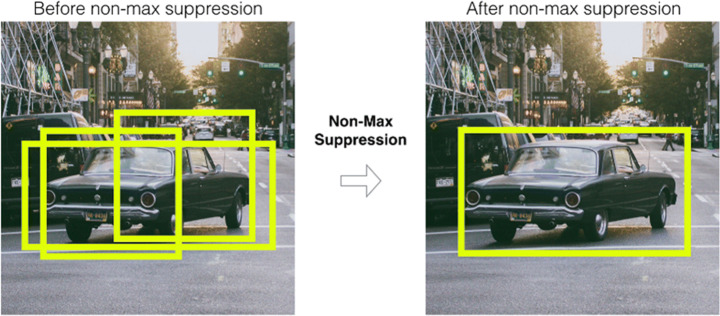
After discarding bounding boxes with the help of some threshold, we are left with a smaller quantity of bounding boxes but this count is also very high. The second criteria for discarding the less relevant bounding boxes is known as non max suppression which is further based upon the IoU. The effect of non max suppression is presented in Fig. 16.
Fig. 16.
The effect of Non-Max Suppression in Object detection using YOLO
Non max suppression internally uses an important concept of Intersection over Union (IoU) which can be computed for two boxes, as illustrated with the help of Fig. 17. First, we select the box having the maximum class score. All other bounding boxes overlapped with the chosen box will be discarded having IoU is greater than some predefined threshold. We repeat these steps until there are no bounding boxes with lower confidence scores than the chosen bounding box.
Fig. 17.
Computational schematic of Intersection over Union (IoU)
YOLO (v1)
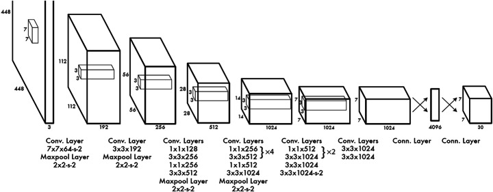
The architecture of YOLO is inspired by the GoogLeNet architecture. It was implemented and tested on VOC Pascal Dataset 2007 and 2012 for an object detection task, and Darknet framework is utilized for the training of model. Herein, inception modules of GoogLeNet are replaced by (1 × 1) convolution followed by (3 × 3) convolutional filters, only the first convolutional layer having a (7 × 7) filter. In YOLO, we have 24 convolution layers followed by 2 fully connected layers as shown in Fig. 18. Out of these 24 convolutional layers, only four convolutional layers are followed by max-pooling layers. The algorithm uses (1 × 1) convolution and global average pooling which standout as highlights of this version.
Fig. 18.
YOLO architecture for object detection and localization [56]
The authors have trained and fine-tuned it initially with first twenty layers followed by an average pooling layer and fully connected layer on ImageNet 2012 dataset for approximately one week. Later on, the model is further fine-tuned for the object detection task after adding four more convolutional layers and two fully connected layers with randomly initialized weights. The activation function being Leaky Rectified Linear Unit (LReLU) for all the convolutional and dense layers except the last layer which has a linear activation function. The final layer is responsible for predicting the class probabilities and bounding boxes coordinates. Large localization error and lower recall in comparison with two stage object detectors may be considered as the two significant drawbacks of this version of YOLO.
A variant of YOLO with lesser model complexity known as Fast YOLO is proposed for faster detection of objects. It has 9 convolutional layers with comparatively lesser filters in those layers. Another variant of YOLO, known as Yolo-lite is proposed, specifically designed for real time object detection on a standard non-GPU system [27]. Authors demonstrate the capability of shallower networks in the object detection without any explicit need of the accelerators. Moreover, they also demonstrate that the presence of batch normalization limits the performance of shallow neural networks in the course of object detection.
Loss function
The sum squared error is used throughout the loss function which is presented using Eq. 6. As we can notice, there are total five terms in the underlying equation wherein notations can be defined as follows:
(xi, yi) is the ground truth center of the bounding box,
(,) is the predicted center of the bounding box,
(wi, hi) is the width and height respectively of the ground truth bounding box,
(,) is the width and height respectively of the predicted bounding box.
The first two terms are related to errors correspond to the differences in positioning of predicted bounding boxes and the ground truth bounding boxes. The deviations have a greater impact on IoU in case of smaller bounding boxes as compared to larger bounding boxes. To address this problem, square root of the width and height of the bounding box is considered instead of width and height directly in the loss function. Third term refers to the prediction difference in the confidence score when the object is present in the corresponding bounding box. In first three terms, is an indicator function, which represents ith grid responsible for predicting the jth bounding box. It will be 1 if the cell contains the object, 0 otherwise. It may happen that ground truth may contain the object in a particular grid cell but the model wrongly predicts there’s no object. Apart from considering the loss when the grid cell contains the object, they also aimed to reduce the loss when there’s no object in the grid cell. It may happen that ground truth may not contain the object in a particular grid cell but the model wrongly predicts there’s an object. Similarly, is an indicator function, which represents ith grid responsible for predicting the jth bounding box. It will be 1 if the cell does not contain the object, 0 otherwise. The last term is classification loss, aimed to minimize the misclassification error. Herein, is an indicator function, which refers to a grid cell containing an object, it will be 1 if the grid cell contains an object and 0 otherwise. The λcoordand λnoobj are the hyperparameters that basically used to avoid divergence of gradients. All the grid cells may not contain the object, the confidence score and thereafter gradients will tend to zero in this case. So, in order to overcome this problem, they tried to maximize the loss of bounding box coordinates when the grid cell contains the object by multiplying the hyperparameter λcoord to the first and second terms and minimize the loss when there is no object in the grid cell by multiplying the hyperparameter λnoobj to the fourth term. In general, high value is assigned to λcoord and low value to λnoobj.
| 6 |
YOLO (v2)
YOLO (v2) is known as an immediate successor of YOLO (v1), utilized for detecting objects for around over 9000 categories [54]. Most of the existing object detection techniques are restricted to classification for limited categories. This is certainly due to scarcity of labelled data for object detection task. So, authors tried the scalability in object detection task for an increased number of categories. To do so, ImageNet and COCO dataset were combined, resulting in more than 9418 categories of object instances. The data for classification problem is huge now, keeping this in mind a hierarchical method known as Word-tree for combining classification and detection is developed. In this section, we discuss the architecture of YOLO (v2) and improvements from the base version.
YOLO (v2) architecture is inspired by VGG and Network-in-Network. It uses darknet-19 framework consisting of 19 convolutional layers and 5 max pooling layers, as illustrated in Fig. 19. In addition, we also observed many 1 × 1 convolution in order to achieve down sampling across the depth of the input volume. It has many additional features when compared to the base version. Various data augmentation techniques such as random crops, rotations, and many more are employed for model training; however, this version struggles in detection of smaller sized objects. Apart from using existing features such as Global average pooling and 1 × 1 convolution, authors also introduced new optimization techniques such as Batch normalization, High resolution classifier, Convolution with anchor boxes, Dimension clusters, Direct location prediction, Fine-Grained features, and Multi-scale training, can be briefly described as follows:
Fig. 19.
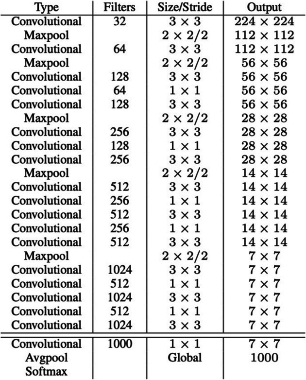
Layer wise architectural operations in Darknet-19 framework [54]
Batch Normalization
During training of neural networks, weights are initialized randomly. As a result, weight matrices of the consecutive layers might adopt different distribution, one distribution may get changed for adopting the changes of the different weight distribution. These changes in the parameters of hidden layers will lead to unnecessary shifts in deeper hidden layers. This problem is termed as Internal Covariate Shift. Outputs of each hidden layer is normalized using Batch normalization to make the consistent distribution of weight matrices across different layers and reduces the problem of internal covariate shift. Besides this, it also acts as a regularization technique and also offers the use of high learning rate. An approximate increase of 2% in mAP is observed by the use of batch normalization.
High Resolution Classifier
In the base version of YOLO, authors trained the model on 224 × 224 sized images for classification and increased the resolution to 448 × 448 for detection. The model had to learn classification and adopt the new resolution. However, in this version, authors trained the model on 448 × 448 sized image for classification before employing it for the detection. Later on, model is fine-tuned for the object detection task and it offers better bounding boxes for high resolution input too. An approximate increase of 4% in mAP is observed by the use of high-resolution classifier.
Convolution with anchor boxes
The fully connected layer is removed from the base version as it was predicting the bounding box coordinates directly, moreover, convolutional layers were responsible for capturing the features. Hand-picked priors are utilized by employing Faster RCNN for predicting the bounding boxes instead of identifying the bounding box coordinates directly. Further, offset prediction makes the model simpler and fast learnable. An approximate increase of 7% in recall is observed by the usage of convolution with anchor boxes, however, 0.3% reduction in mAP is also noticed.
Dimension clusters
Unlike hand-picked anchor boxes in YOLO, the anchor boxes using k-means clustering are extracted. Better shaped anchor boxes may provide quick start and offers improved model training and performance.
Direct location prediction
YOLO had two issues, firstly, handpicked dimension priors which was addressed by use of k-means clustering and secondly, model instability at the time of bounding box prediction. Random initialization is considered as the biggest hurdles in predicting genuine offsets. Instead, we predict the location coordinates relative to the grid-cell locations. This added feature increased the mAP by 5%.
Fine-grained features
YOLO predicts larger objects easily with a 13 × 13 feature map. However, if the image has smaller objects, it fails to recognize effectively. Using the idea of skip connections in ResNet, as shown in the Fig. 20, higher resolution features are concatenated with the lower resolution features in consecutive channels. The reshaping is performed i.e., 26 × 26 × 512 features map is converted into 13 × 13 × 2048 features map then concatenated it with the model hence predicted output size is 13 × 13 × 1024. The resultant tensor shape would be 13 × 13 × 3072 for which filters were applied. Adding a passthrough layer has increased mAP by 1%.
Fig. 20.
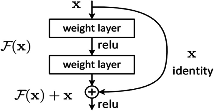
Skip connections in the ResNet Module [25]
Multi-scale training
After exclusion of fully connected layers, YOLO (v2) can now operate on any dimension ranging from 320 × 320 to 608 × 608. The model randomly chooses the new dimension which is multiple of 32 for every 10 epochs. This gives the flexibility to the model to predict on various dimensions.
YOLO (v3)
The base version of YOLO didn’t have a solution for localization errors and second version failed in detecting the smaller sized objects. The third version of YOLO tries to overcome aforementioned drawbacks and provides an efficient way for detecting objects with an improved performance while trained and evaluated on the COCO dataset [55]. As this version outperforms for smaller sized objects, however, suffers in producing accurate results for medium and large sized objects.
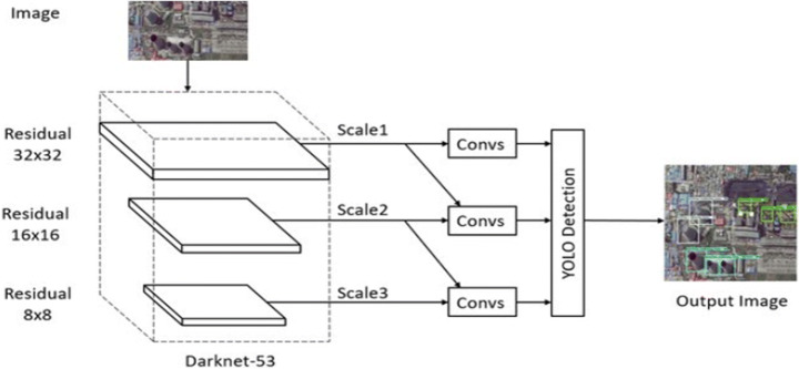
This architecture is based on Darkent-53 framework, a network that uses 3 × 3 and 1 × 1 convolutional filter along with some shortcut connections, significantly larger and powerful architecture with 53 convolutional layers. It is twice faster than ReNet-152 while not compromising with the performance. The underlying generic architecture for YOLO (v3) is demonstrated in Fig. 21.
Fig. 21.
Architecture of YOLO (v3) [81]
YOLO (v3) is inspired by Feature Pyramid Network (FPN). It incorporates heuristics like residual blocks, skip connections, and up-sampling similar to FPN. It uses Darknet53 as a base network, upon that adding 53 more layers to make it easy for object detection. Like FPN, YOLO (v3) also uses (1 × 1) convolution on feature maps to detect objects. It generates feature maps at three different scales. Specifically, it down-samples the input at 3 different scales by a factor of 32, 16, and 8. Initially, after 81 series of convolutions, in the 82nd layer after applying a stride of 32, the resultant tensor is a 13 × 13 feature map that is utilized for detection using (1 × 1) convolution. Secondly, the detection is made after the 94th layer after applying a stride of 16. Few convolutions on the 79th layer is added, after which it is concatenated with 61st layer on 2x up-sampling, yields a 26 × 26 feature map. Finally, the 106th layer is involved in the detection using a 52 × 52 feature map after applying a stride of 8. Following the same process, adding few convolutions to the 91st layer and combining with the 36th layer using (1 × 1) kernel, the down-sampled feature maps are concatenated to Up-sampled feature maps at different places to extract fine-grained features for detecting smaller objects of various dimensions. Conclusively different feature maps viz. 52 × 52, 13 × 13, and 26 × 26 are utilized for detecting large, smaller, and medium-sized objects respectively.
YOLO (v4)
The fourth version of YOLO series was drafted by Alexey Bochkovskiy, Chien-Yao Wang and Hong-Yuan Mark Liao [5]. This version introduces new methods, showcases a variety of complex and powerful techniques. This version is faster and more accurate than all the previous versions. The model aimed to produce an object detector for production systems. Authors segregated the problem statement and approaches into several segments then they have proposed a variety of methodologies which can best fit the available resources. Firstly, an input image is provided of dimension H × W, where H represents height and W represents width. Secondly, a series of convolutions which extracts features through powerful networks like VGG16, Darknet53, ResNet50, and other variants which they termed as backbone. Thirdly, a neck which can be utilized to extract features at different scales such as Feature Pyramid Network (FPN), Path Aggregation Network (PAN), and other variants which is the composition of connections between bottom-up and top-down pathways. Finally, the prediction of anchor boxes using single-stage detectors like YOLO which have dense layers or using two-stage detectors like Faster R-CNN which have sparse predictions act as a head.
On the architectural side, the authors have compared CSPResNeXt50, CSPDarknet53, and EfficientNetB3 for construction of YOLO (v4) architecture. CSPDarknet53, a network with 29 convolution layers with 3 × 3 filters and approximately 27.6 million parameters, is chosen as backbone that outperformed the remaining architectures wherein CSP stands for Cross-stage partial connections. CSPNets help in rich gradient combination with minimal computation cost [73], as illustrated in Fig. 22.
Fig. 22.
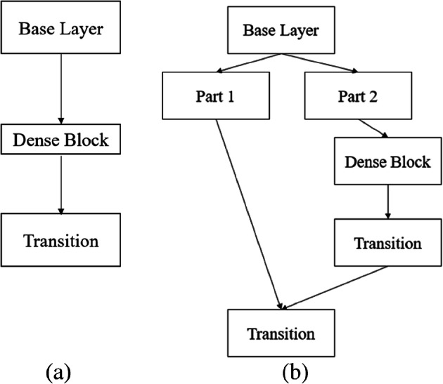
CSPNet vs DenseNet architecture utilized in YOLO-v4 [73]. a CSPNet b DenseNet
The ImageNet pretrained model for classification with the underlying dataset as COCO for experimentation is utilized [73]. Authors used Spatial Pyramid Pooling (SPP) which was also used by RCNN. Here, a CNN followed by fully connected layers has a restriction over input and output volume. However, this version ensures handling of any input irrespective of the dimension without resizing or reshaping it. SPP is placed between a CNN and fully connected layer which maps any input size to fixed size output. This gives an option to detect objects of an image of varied size, moreover, genetic algorithm is applied for hyperparameters tuning. In addition, Path Aggregation Network (PAN) is preferred over Feature Pyramid Network (FPN) where PAN is a bottom-up path augmentation that uses Adaptive feature pooling which works similar to FPN.
Summarization and future research directions
Object Detection comprises the fundamental tasks such as object classification, localization, and segmentation. Object detection and related tasks are classified in two categories viz. single stage and two stages. In this paper, we explored two stage object detectors viz. RCNN, Fast-RCNN, and Faster-RCNN along with their important applications. We majorly reviewed single stage object detectors especially YOLOs, their architectural advancements, underlying pretrained CNN architectures, and loss function in details. We presented different aspects and optimizations carried out in the successive versions of YOLOs along with all the underlying concepts. Moreover, we presented the challenges and motivations behind the specific review of single stage object detectors. YOLOs are performing significantly better in comparison with their counterpart two stage object detectors in terms of detection accuracy and inference time.
To the best of our knowledge, this is the first review covering single stage object detectors especially YOLOs. The following tables provide the summarization of the entire paper in terms of comparative illustrations, results, and applications. Table 3 summarizes the differences between single- and two-stage object detectors. Single stage object detectors are mainly designed for real time object detection; however, they are lagging in the performance metrics to the two stage object detectors. Moreover, YOLOs make comparatively fewer errors in the identification of the background, quick boost in the performance is observed, if YOLOs are utilized for background detection in the two stage object detection algorithms. The combination of YOLO and Fast-RCNN outperform to the each of these standalone architecture on Pascal VOC dataset.
Table 3.
Comparison of Two-stage (R-CNN & Successors) and Single-stage detectors (YOLOs)
| Features | R-CNN and its successors | YOLO and its successors |
|---|---|---|
| Region proposals | Region proposals (or ROI) are generated using Selective search algorithm | Region proposals are generated by a single convolutional network. |
| Feature extraction (Backbone network) | The backbone network is a heavyweight and time consuming. | The backbone network is a lightweight and faster feature extractor. |
| Number of stages and their role | First stage extracts region proposals. Second stage extracts feature vectors, thereafter detections. | A single stage network predicts the bounding boxes offsets, confidence score and class conditional probabilities |
| Speed and accuracy | Higher accuracy and low speed. | Faster detection and accuracy nearer to two stage object detectors. |
| Computational cost | They require powerful resources for computation and are computationally expensive. | Not necessary for powerful resources for computation and are less expensive. |
| Performance | They are efficient for detecting smaller and larger objects. | They have mostly shown poor performance for detecting smaller objects and have been efficient for larger objects. |
Table 4 summarizes the comparative analysis among the different version of YOLOs. Darknets were majorly adopted for the implementation of YOLOs. Each successor has come up with some type of optimizations over its predecessor, as described in the previous section. With the help of multi scale training, YOLO-v2 offers better detection on varying sized objects with an easy trade-off between the model performance and model inferences. A unified method is presented using the joint training for detection and classification as well. YOLO-v3 is better detector, fast, and accurate, necked by feature pyramid network. YOLO-v4 is also an attempt to better deal with the trade-off between the accuracy and speed of the model by introducing several universal optimization features of CNNs. With this journey of YOLOs, we can conclude that it is an incremental approach of the betterment of the trade-off between speed and accuracy. Table 5 illustrates the performance outcomes of different versions of YOLOs in terms of processing speed and average precision. Depending upon the requirement of the applications and nature of the underlying dataset, one should adopt any specific version of single stage, two stage, or a combination of both of these. Finally, Table 6 presents some of the important applications of YOLOs based detection and recognition.
Table 4.
Comparison of YOLO and its successors
| Yolo version | Architecture (Backbone) | Neck | Anchor boxes | Features |
|---|---|---|---|---|
| Yolo(v1) | Darknet (GoogLeNet 24 layers) | – | Handpicked | 1 × 1 convolutions, global average pooling, linear activation and leaky ReLU. |
| Yolo(v2) | Darknet-19 | – | 5 anchor boxes using K-means clustering. | Batch Normalization, high resolution classifier, convolution with anchor boxes, dimension clusters, direct location prediction, fine-grained features and multi-scale training. |
| Yolo(v3) | Darknet-53 | Feature Pyramid Networks | 9 anchor boxes using K-means clustering. | Independent Logistic classifiers, multi-scale training and predictions. |
| Yolo(v4) | CSP Darknet-53 | Path Aggregation Network | 9 anchor boxes using K-means clustering. | Spatial Pyramid Pooling (SPP), DropBlock regularization, Mish activation, ReLU6, Class label smoothing and Cross Mini-Batch Normalization. |
Table 5.
Summarization of Results of YOLO, variants, and successors
| Yolo version | Underlying Dataset | Processing Speed – frames per second (fps) | Performance Measures (mAP) |
|---|---|---|---|
| Yolo(v1) | PASCAL VOC 2007 + 2012 | 45 | 63.4 |
| Fast Yolo | PASCAL VOC 2007 + 2012 | 155 | 52.7 |
| Yolo(v2) | PASCAL VOC 2007 + 2012 | 40 | 78.6 |
| Yolo - lite | PASCAL VOC 2007 + 2012 | 21 | 33.77 |
| Yolo(v3) | MS COCO | 20 | 57.9 |
| Yolo(v4) | MS COCO | 33 | 65.7 |
Table 6.
Applications of different versions of YOLOs
| Ref. | Model Based on | Application | Key characteristics | Performance Metrics |
|---|---|---|---|---|
| [79] | YOLO v1 | Garbage Detection and Classification |
• YOLO using Variational Autoencoder to achieve higher accuracy • Model comprise of convolutional feature extractor, predictor, and decoder |
• Correct rate - 69.70% (60 fps) |
| [87] | YOLO v1 | Robot based Binocular intelligent system |
• YOLO-LITE utilized for target detection • Raspberry Pi 3B+ applied for camera processing |
• Average detection accuracy - 80% |
| [52] | YOLO v1 | Teat detection |
• Haar-cascade applied for object detection • YOLO employed for custom object detection |
NA |
| [35] | YOLO v2 | Multivehicle detection |
• Applied improved YOLO-voc as per change identified in traffic flow and target scene • Parameter fine-tuning based on vehicle characteristics |
• Detection rate - 98.6% |
| [46] | YOLO v2 | Medical face mask detection |
• ResNet-50 as transfer learning model YOLO v2 adopted for face mask detection |
• Average precision - 81% |
| [84] | YOLO v2 | Image and color recognition |
• Target recognition using YOLO v2 for identifying and locating traffic light • HSV applied to transform in color space |
• Recognition rate - 76% - 100% |
| [7] | YOLO v2 | Shuttlecock detection |
• Modified Tiny YOLO v2 is applied to capture sematic information • Badminton robot cum vision system |
• Precision - 96.3% |
| [9] | YOLO v3 | pole detection and counting in distribution network |
• YOLO for rapid detection • CNN for image detection |
• Precision - above 90% |
| [47] | YOLO v3 | Object detection in real-rime for embedded system |
• Darknet-53 applied as a feature extractor • Pyramid network to enhance the performance of multi-scale object detection |
• mAP-50 of 52.1 • AP: 0.5: 0.95 of 29.8 at the speed of 67 fps |
| [36] | YOLO v3 | Target detection on PCB |
• Darknet-53 applied as a feature extractor • Modification in output layers of YOLO |
• mAP - 93.07% |
| [30] | YOLO v4 | Human Detection |
• Usage of arial thermal imaging • Multiscale object detection |
• mAP – 91% |
| [28] | YOLO v4 | Ship detection |
• Highspeed ship detection using colored SAR input • Multichannel fusion of SAR images fusion network |
• AP - 90.30% |
| [76] | YOLO v4 | Apple flower detection |
• YOLO v4 model with CSP Darknet53 • Pruning of model using channel pruning |
• mAP - 97.31% |
Numerous researches are being carried out on in further improvements of YOLO (v4). Next version of YOLO i.e., YOLO (v5) is also proposed but we purposefully not included it in this review. YOLOs are being rigorously employed in various real time object tracking such as self-driving cars. Advancements in the convolutional neural networks should be rigorously experimented in further improvement in single stage object detectors. With the architectural advancements of CNN, features’ extraction process can be made more robust by employing various advance types of convolutions such as tiled-, transposed-, and dilated-convolution. Depending on the nature of applications and underlying datasets, these convolutions may be utilized to further improve the process. Models trained for one particular task may not perform well on other similar tasks, resulting non-generalizability of the model for the data it has not seen before. Different types of regularizations such as LP-Normalization, dropouts, and drop-connects should be experimented for better generalized models. Generally, deep models take huge amount of time for model training due to the large dataset size and model complexity, various optimizations techniques such as usage of Fast Fourier Transform, low precision, weight compression, etc. should be explored for the faster convergence of the single stage object detectors.
Acknowledgments
The authors, thanks to all the anonymous reviewers of Multimedia Tools and Applications Journal for their constructive remarks and fruitful suggestions to improve the manuscript.
Declarations
Competing interests
We do not have any conflict of interest related to the manuscript.
Footnotes
Publisher’s note
Springer Nature remains neutral with regard to jurisdictional claims in published maps and institutional affiliations.
Contributor Information
Tausif Diwan, Email: tdiwan@iiitn.ac.in.
G. Anirudh, Email: ganirudhani90@gmail.com
Jitendra V. Tembhurne, Email: jtembhurne@iiitn.ac.in
References
- 1.Agarwal S, Terrail JO, Jurie F (2018) Recent advances in object detection in the age of deep convolutional neural networks. arXiv preprint arXiv:1809.03193. 10.48550/arXiv.1809.03193
- 2.Albelwi S, Mahmood A. A framework for designing the architectures of deep convolutional neural networks. Entropy. 2017;19(6):242. doi: 10.3390/e19060242. [DOI] [Google Scholar]
- 3.Bengio Y, Courville AC, Vincent P (2012) Unsupervised feature learning and deep learning: a review and new perspectives. CoRR, abs/1206.5538, 1(2665)
- 4.Bhattacharya S, Maddikunta PKR, Pham QV, Gadekallu TR, Chowdhary CL, Alazab M, Piran MJ (2021) Deep learning and medical image processing for coronavirus (COVID-19) pandemic: a survey. Sustain Cities Soc 65:102589. 10.1016/j.scs.2020.102589 [DOI] [PMC free article] [PubMed]
- 5.Bochkovskiy A, Wang CY, Liao HY (2020) YOLOv4: optimal speed and accuracy of object detection. arXiv preprint arXiv:2004.10934
- 6.Borisyuk F, Gordo A, Sivakumar V (2018) Rosetta: large scale system for text detection and recognition in images. In proceedings of the 24th ACM SIGKDD international conference on knowledge discovery data mining pp 71-79
- 7.Cao Z, Liao T, Song W, Chen Z, Li C (2021) Detecting the shuttlecock for a badminton robot: a YOLO based approach. Expert Syst Appl 164:113833. 10.1016/j.eswa.2020.113833
- 8.Che Z, Purushotham S, Cho K, Sontag D, Liu Y. Recurrent neural networks for multivariate time series with missing values. Sci Rep. 2018;8(1):1–12. doi: 10.1038/s41598-018-24271-9. [DOI] [PMC free article] [PubMed] [Google Scholar]
- 9.Chen B, Miao X (2020) Distribution line pole detection and counting based on YOLO using UAV inspection line video. J Electr Eng Technol 15(1):441–448. 10.1007/s42835-019-00230-w
- 10.Chen K, Franko K, Sang R (2021) Structured model pruning of convolutional networks on tensor processing units. ArXiv preprint arXiv:210704191. 10.48550/arXiv.2107.04191
- 11.Choi H, Ryu S, Kim H (2018) Short-term load forecasting based on ResNet and LSTM. In IEEE international conference on communications, control, and computing Technologies for Smart Grids (SmartGridComm), pp 1-6
- 12.Cook A (2017) Global average pooling layers for object localization. https://alexisbcook.github.io/2017/globalaverage-poolinglayers-for-object-localization/. Accessed 19 Aug 2019
- 13.Detection or localization and segmentation (n.d.) https://www.oreilly.com/library/view/deep-learning-for/9781788295628/4fe36c40-7612-44b8-8846-43c0c4e64157.xhtml
- 14.Everingham M, Eslami SA, Van Gool L, Williams CK, Winn J, Zisserman A. The pascal visual object classes challenge: a retrospective. Int J Comput Vis. 2015;111(1):98–136. doi: 10.1007/s11263-014-0733-5. [DOI] [Google Scholar]
- 15.Felzenszwalb P, McAllester D, Ramanan D (2008) A discriminatively trained, multiscale, deformable part model In IEEE conference on computer vision and pattern recognition 2008, pp 1–8
- 16.Fu CY, Liu W, Ranga A, Tyagi A, Berg AC (2017) Dssd: Deconvolutional single shot detector. arXiv preprint arXiv:1701.06659
- 17.Gadekallu TR, Rajput DS, Reddy MPK, Lakshmanna K, Bhattacharya S, Singh S, Alazab M (2020) A novel PCA–whale optimization-based deep neural network model for classification of tomato plant diseases using GPU. J Real Time Image Process 18(4):1383–1396. 10.1007/s11554-020-00987-8
- 18.Gadekallu TR, Alazab M, Kaluri R, Maddikunta PKR, Bhattacharya S, Lakshmanna K, Parimala M (2021) Hand gesture classification using a novel CNN-crow search algorithm. Complex Intell Syst 7(4):1855–1868. 10.1007/s40747-021-00324-x
- 19.Gavali P, Banu JS (2019) Deep convolutional neural network for image classification on CUDA platform. In: Deep learning and parallel computing environment for bioengineering systems, pp 99–122
- 20.Girshick R (2015) Fast r-cnn. In proceedings of the IEEE international conference on computer vision 2015, pp 1440–1448
- 21.Girshick R, Donahue J, Darrell T, Malik J (2014) Rich feature hierarchies for accurate object detection and semantic segmentation. In: Proceedings of the IEEE conference on computer vision and pattern recognition, pp 580–587
- 22.Google Lens – Wikipedia (n.d.), https://en.wikipedia.org/wiki/Google_Lens. Accessed 06 Aug 2020
- 23.Gu J, Wang Z, Kuen J, Ma L, Shahroudy A, Shuai B, Liu T, Wang X, Wang G, Cai J, Chen T (2018) Recent advances in convolutional neural networks. Pattern Recogn 77:354–377. 10.1016/j.patcog.2017.10.013
- 24.Han C, Gao G, Zhang Y (2019) Real-time small traffic sign detection with revised faster-RCNN. Multimed Tools Appl 78(10):13263–13278. 10.1007/s11042-018-6428-0
- 25.He K, Zhang X, Ren S, Sun J (2016) Deep residual learning for image recognition. In proceedings of the IEEE conference on computer vision and pattern recognition, pp 770-778
- 26.Hossain S, Lee DJ. Deep learning-based real-time multiple-object detection and tracking from aerial imagery via a flying robot with GPU-based embedded devices. Sensors. 2019;19(15):3371. doi: 10.3390/s19153371. [DOI] [PMC free article] [PubMed] [Google Scholar]
- 27.Huang R, Pedoeem J, Chen C (2018) YOLO-LITE: a real-time object detection algorithm optimized for non-GPU computers. In: 2018 IEEE international conference on big data (big data), pp 2503–2510. 10.1109/BigData.2018.8621865
- 28.Jiang J, Fu X, Qin R, Wang X, Ma Z. High-speed lightweight ship detection algorithm based on YOLO-V4 for three-channels RGB SAR image. Remote Sens. 2021;13(10):1909. doi: 10.3390/rs13101909. [DOI] [Google Scholar]
- 29.Jiao L, Zhang F, Liu F, Yang S, Li L, Feng Z, Qu R (2019) A survey of deep learning-based object detection. IEEE Access 7:128837–128868. 10.1109/ACCESS.2019.2939201
- 30.Kannadaguli P (2020) YOLO v4 based human detection system using aerial thermal imaging for UAV based surveillance applications. In 2020 international conference on decision aid sciences and application (DASA) pp 1213-1219
- 31.Khan A, Sohail A, Zahoora U, Qureshi AS (2020) A survey of the recent architectures of deep convolutional neural networks. Artif Intell Rev 53(8):5455–5516. 10.1007/s10462-018-9633-3
- 32.Kim J, Kim J, Thu HLT, Kim H (2016) Long short term memory recurrent neural network classifier for intrusion detection. In: 2016 international conference on platform technology and service (PlatCon), pp 1–5. 10.1109/PlatCon.2016.7456805
- 33.Lai S, Xu L, Liu K, Zhao J (2015) Recurrent convolutional neural networks for text classification. In: Twenty-ninth AAAI conference on artificial intelligence
- 34.Lee HJ, Chung JH (1995) Hand gesture recognition using orientation histogram. In IEEE Region 10 Conference TENCON 99. Multimed Technol Asia-Pacific Inform Infrastruct (Cat. No. 99CH37030) 2:1355–1358. 10.1109/TENCON.1999.818681
- 35.Li X, Liu Y, Zhao Z, Zhang Y, He L (2018) A deep learning approach of vehicle multitarget detection from traffic video J Adv Transport 2018. 10.1155/2018/7075814
- 36.Li J, Gu J, Huang Z, Wen J. Application research of improved YOLO V3 algorithm in PCB electronic component detection. Appl Sci. 2019;9(18):3750. doi: 10.3390/app9183750. [DOI] [Google Scholar]
- 37.Liang M, Hu X (2015) Recurrent convolutional neural network for object recognition. In: Proceedings of the IEEE conference on computer vision and pattern recognition, pp 3367–3375. 10.1109/CVPR.2015.7298958
- 38.Liao S, Wang J, Yu R, Sato K, Cheng Z (2017) CNN for situations understanding based on sentiment analysis of twitter data. Procedia Comput Sci 111:376-381. 10.1016/j.procs.2017.06.037
- 39.Lin M, Chen Q, Yan S (2013) Network in network. arXiv preprint arXiv:1312.4400. 10.48550/arXiv.1312.4400
- 40.Lin TY, Maire M, Belongie S, Hays J, Perona P, Ramanan D, Dollár P, Zitnick CL (2014) Microsoft coco: common objects in context. In: European Conf Comput Vis, pp 740–755. 10.48550/arXiv.1405.0312
- 41.Lin TY, Goyal P, Girshick R, He K, Dollár P (2017) Focal loss for dense object detection. In: Proceedings of the IEEE international conference on computer vision, pp 2980–2988. 10.48550/arXiv.1708.02002
- 42.Lin TY, Dollár P, Girshick R, He K, Hariharan B, Belongie S (2017) Feature pyramid networks for object detection. In: Proceedings of the IEEE conference on computer vision and pattern recognition, pp 2117–2125
- 43.Liu W, Anguelov D, Erhan D, Szegedy C, Reed S, Fu CY, Berg AC (2016) Ssd: single shot multibox detector. European Conf Comput Vis 2016:21–37. 10.48550/arXiv.1512.02325
- 44.Liu L, Ouyang W, Wang X, Fieguth P, Chen J, Liu X, Pietikäinen M. Deep learning for generic object detection: a survey. Int J Comput Vis. 2020;28(2):261–318. doi: 10.1007/s11263-019-01247-4. [DOI] [Google Scholar]
- 45.Liu L, Ouyang W, Wang X, Fieguth P, Chen J, Liu X, Pietikäinen M (2020) Deep learning for generic object detection: a survey. Int J Comput Vis 128(2):261–318. 10.48550/arXiv.1809.02165
- 46.Loey M, Manogaran G, Taha MHN, Khalifa NEM. Fighting against COVID-19: a novel deep learning model based on YOLO-v2 with ResNet-50 for medical face mask detection. Sustain Cities Soc. 2021;65:102600. doi: 10.1016/j.scs.2020.102600. [DOI] [PMC free article] [PubMed] [Google Scholar]
- 47.Mao QC, Sun HM, Liu YB, Jia RS. Mini-YOLOv3: real-time object detector for embedded applications. IEEE Access. 2019;7:133529–133538. doi: 10.1109/ACCESS.2019.2941547. [DOI] [Google Scholar]
- 48.Mezaal MR, Pradhan B, Sameen MI, Shafri M, Zulhaidi H, Yusoff ZM (2017) Optimized neural architecture for automatic landslide detection from high resolution airborne laser scanning data. Appl Sci 7(7):730. 10.3390/app7070730
- 49.Morris T (2004) Computer Vision and Image Processing, Palgrave Macmillan Ltd, 1st edition, pp 1–320
- 50.Nash W, Drummond T, Birbilis N. A review of deep learning in the study of materials degradation. Mater Degrad. 2018;2(1):1–2. [Google Scholar]
- 51.Quang D, Xie X (2016) DanQ: a hybrid convolutional and recurrent deep neural network for quantifying the function of DNA sequences. Nucleic Acids Res 44(11):e107–e107. 10.1093/nar/gkw226 [DOI] [PMC free article] [PubMed]
- 52.Rastogi A, Ryuh BS. Teat detection algorithm: YOLO vs Haar-cascade. J Mech Sci Technol. 2019;33(4):1869–1874. doi: 10.1007/s12206-019-0339-5. [DOI] [Google Scholar]
- 53.Rather AM, Agarwal A, Sastry VN. Recurrent neural network and a hybrid model for prediction of stock returns. Expert Syst Appl. 2015;42(6):3234–3241. doi: 10.1016/j.eswa.2014.12.003. [DOI] [Google Scholar]
- 54.Redmon J, Farhadi A (2017) YOLO9000: better, faster, stronger. In: Proceedings of the IEEE conference on computer vision and pattern recognition 2017, pp 7263–7271. 10.48550/arXiv.1612.08242
- 55.Redmon J, Farhadi A (2018) Yolov3: an incremental improvement. arXiv preprint arXiv:1804.02767
- 56.Redmon J, Divvala S, Girshick R, Farhadi A (2016) You only look once: unified, real-time object detection. In proceedings of the IEEE conference on computer vision and pattern recognition, pp 779-788
- 57.Ren S, He K, Girshick R, Sun J (2015) Faster r-cnn: towards real-time object detection with region proposal networks. Adv Neural Inform Process Syst:91–99 [DOI] [PubMed]
- 58.Rey J (2017) Object detection with deep learning: the definitive guide
- 59.Sak H, Senior A, Rao K, Beaufays F (2015) Fast and accurate recurrent neural network acoustic models for speech recognition. arXiv preprint arXiv:1507.06947
- 60.Raj Sakthi (2013) Talented Mr. 1X1: Comprehensive look at 1X1 Convolution in Deep Learning, Medium, 2013
- 61.Sermanet P, Eigen D, Zhang X, Mathieu M, Fergus R, LeCun Y (2013) Overfeat: integrated recognition, localization and detection using convolutional networks. arXiv preprint arXiv:1312.6229
- 62.Sharma V, Mir RN (2019) Saliency guided faster-RCNN (SGFr-RCNN) model for object detection and recognition. J King Saud Univ - Comput Inf Sci. 10.1016/j.jksuci.2019.09.012
- 63.Shi Y, Li Y, Wei X, Zhou Y (2017) A faster-rcnn based chemical fiber paper tube defect detection method. In: 2017 5th international conference on enterprise systems (ES), pp 173–177. 10.1109/ES.2017.35
- 64.Simonyan K, Zisserman A (2014) Very deep convolutional networks for large-scale image recognition. arXiv preprint arXiv:1409. 10.48550/arXiv.1409.1556
- 65.Szegedy C, Liu W, Jia Y, Sermanet P, Reed S, Anguelov D, Erhan D, Vanhoucke V, Rabinovich A (2015) Going deeper with convolutions. In: Proceedings of the IEEE conference on computer vision and pattern recognition, pp 1–9. 10.48550/arXiv.1409.4842
- 66.Thai LH, Hai TS, Thuy NT. Image classification using support vector machine and artificial neural network. Int J Inform Technol Comput Sci. 2012;4(5):32–38. [Google Scholar]
- 67.Tsang S-H (2018) Review: Inception-v4 - Evolved From GoogLeNet, Merged with ResNet Idea (Image Classification), towards data science
- 68.Ujjwalkarn (2016) An Intuitive Explanation of Convolutional Neural Networks, the data science blog
- 69.Vasan D, Alazab M, Wassan S, Naeem H, Safaei B, Zheng Q (2020) IMCFN: image-based malware classification using fine-tuned convolutional neural network architecture. Comput Netw 171:107138. 10.1016/j.comnet.2020.107138
- 70.Viola P, Jones MJ (2004) Robust real-time face detection. Int J Comput Vis 57(2):137–154. 10.1023/B:VISI.0000013087.49260.fb
- 71.Voulodimos A, Doulamis N, Doulamis A, Protopapadakis E. Deep learning for computer vision: a brief review. Comput Intell Neurosci. 2018;2018:1–13. doi: 10.1155/2018/7068349. [DOI] [PMC free article] [PubMed] [Google Scholar]
- 72.Wang X, Zhang Q (2018) The building area recognition in image based on faster-RCNN. In 2018 international conference on sensing diagnostics prognostics and control (SDPC) pp 676-680
- 73.Wang CY, Mark Liao HY, Wu YH, Chen PY, Hsieh JW, Yeh IH (2020) CSPNet: a new backbone that can enhance learning capability of CNN. In: Proceedings of the IEEE/CVF conference on computer vision and pattern recognition workshops, pp 390–391
- 74.Wei H, Kehtarnavaz N. Semi-supervised faster RCNN-based person detection and load classification for far field video surveillance. Mach Learn Knowl Extraction. 2019;1(3):756–767. doi: 10.3390/make1030044. [DOI] [Google Scholar]
- 75.Wei D, Wang B, Lin G, Liu D, Dong Z, Liu H, Liu Y (2017) Research on unstructured text data mining and fault classification based on RNN-LSTM with malfunction inspection report. Energies 10(3):406. 10.3390/en10030406
- 76.Wu D, Lv S, Jiang M, Song H (2020) Using channel pruning-based YOLO v4 deep learning algorithm for the real-time and accurate detection of apple flowers in natural environments. Comput Electron Agric 178:105742. 10.1016/j.compag.2020.105742
- 77.Xiang J, Dong T, Pan R, Gao W. Clothing attribute recognition based on RCNN framework using L-Softmax loss. IEEE Access. 2020;8:48299–48313. doi: 10.1109/ACCESS.2020.2979164. [DOI] [Google Scholar]
- 78.Xu N, Liu AA, Wong Y, Zhang Y, Nie W, Su Y, Kankanhalli M (2018) Dual-stream recurrent neural network for video captioning. IEEE Trans Circuits Syst Vid Technol 29(8):2482–2493. 10.1109/TCSVT.2018.2867286
- 79.Ye A, Pang B, Jin Y, Cui J (2020) A YOLO-based neural network with VAE for intelligent garbage detection and classification. In 2020 3rd international conference on algorithms computing and artificial intelligence pp 1-7
- 80.Zaytar MA, El Amrani C. Sequence to sequence weather forecasting with long short-term memory recurrent neural networks. Int J Comput Appl. 2016;143(11):7–11. [Google Scholar]
- 81.Zhang H, Deng Q. Deep learning-based fossil-fuel power plant monitoring in high resolution remote sensing images: a comparative study. Remote Sens. 2019;11(9):1117. doi: 10.3390/rs11091117. [DOI] [Google Scholar]
- 82.Zhang Y, Jiang Y, Tong Y. Study of sentiment classification for Chinese microblog based on recurrent neural network. Chin J Electron. 2016;25(4):601–607. doi: 10.1049/cje.2016.07.002. [DOI] [Google Scholar]
- 83.Zhang XY, Yin F, Zhang YM, Liu CL, Bengio Y. Drawing and recognizing chinese characters with recurrent neural network. IEEE Trans Pattern Anal Mach Intell. 2017;40(4):849–862. doi: 10.1109/TPAMI.2017.2695539. [DOI] [PubMed] [Google Scholar]
- 84.Zhang X, Qiu Z, Huang P, Hu J, Luo J (2018) Application research of YOLO v2 combined with color identification. In 2018 international conference on cyber-enabled distributed computing and knowledge discovery (CyberC) pp 138-1383
- 85.Zhang S, Wen L, Lei Z, Li SZ (2020) RefineDet++: single-shot refinement neural network for object detection. IEEE Trans Circuits Syst Video Technol 31(2):674–687. 10.1109/TCSVT.2020.2986402
- 86.Zhao Q, Sheng T, Wang Y, Tang Z, Chen Y, Cai L, Ling H. M2det: a single-shot object detector based on multi-level feature pyramid network. Proceed AAAI Conf Artif Intell. 2019;33:9259–9266. [Google Scholar]
- 87.Zheng Y, Ge J (2021) Binocular intelligent following robot based on YOLO-LITE. In MATEC web of conferences (Vol 336 p 03002) EDP sciences


