A Multiscale Model of COVID-19 Dynamics

Abstract

COVID-19, caused by the infection of severe acute respiratory syndrome coronavirus 2 (SARS-CoV-2), has been a global pandemic and created unprecedented public health challenges throughout the world. Despite significant progresses in understanding the disease pathogenesis and progression, the epidemiological triad of pathogen, host, and environment remains unclear. In this paper, we develop a multiscale model to study the coupled within-host and between-host dynamics of COVID-19. The model includes multiple transmission routes (both human-to-human and environment-to-human) and connects multiple scales (both the population and individual levels). A detailed analysis on the local and global dynamics of the fast system, slow system and full system shows that rich dynamics, including both forward and backward bifurcations, emerge with the coupling of viral infection and epidemiological models. Model fitting to both virological and epidemiological data facilitates the evaluation of the influence of a few infection characteristics and antiviral treatment on the spread of the disease. Our work underlines the potential role that the environment can play in the transmission of COVID-19. Antiviral treatment of infected individuals can delay but cannot prevent the emergence of disease outbreaks. These results highlight the implementation of comprehensive intervention measures such as social distancing and wearing masks that aim to stop airborne transmission, combined with surface disinfection and hand hygiene that can prevent environmental transmission. The model also provides a multiscale modeling framework to study other infectious diseases when the environment can serve as a reservoir of pathogens.

Introduction

In late December 2019, highly contagious pneumonia of unknown etiology was first reported in Wuhan, China (Zhu et al. 2020). A novel strain of coronavirus was isolated from patients and later named severe acute respiratory syndrome coronavirus 2 (SARS-CoV-2). Since then, the Coronavirus Disease 2019 (COVID-19) has spread to over 210 countries and territories, creating unprecedented public health challenges throughout the world. As of January 12, 2021, more than 91 million cases and 1.9 million deaths had been reported. Despite many theoretical, experimental and clinical studies, our current knowledge on the fundamental mechanisms of COVID-19 transmission and infection remains limited.

Mathematical modeling provides a powerful theoretical means to study COVID-19. A large number of mathematical and statistical models have been proposed (e.g., Kucharski et al. 2020; He et al. 2020; Li et al. 2020; Liu et al. 2020a, c; Tang et al. 2020; Weitz et al. 2020; Wu et al. 2020a, b; Zhao and Feng 2020; Hellewell et al. 2020; Chen et al. 2020; Olabode et al. 2021; Musa et al. 2022). Almost all these models are concerned with the transmission and spread of the disease (i.e., the between-host dynamics) at the population level. On the other hand, very little modeling effort has been devoted to the within-host dynamics of SARS-CoV-2. When the coronavirus enters the human body, there are complicated interactions between the pathogen and host cells taking place, which directly shapes the disease risk and infection severity for the individual hosts and which, in a collective manner, may subsequently impact the epidemic patterns (Liu et al. 2020b; He et al. 2020). Due to the inadequate investigation of the within-host dynamics of COVID-19 and their connection to the population-level epidemics, there are several fundamental questions that remain unanswered or only partially answered at present; for example, how does the viral load change inside the human body, what are the short-term and long-term interactions between SARS-CoV-2 and the host cells, and how does the within-host pathogen development affect the population-level disease transmission and spread?

As a pilot study to address these questions, we develop a multiscale modeling framework in this paper to investigate the between-host and within-host dynamics of COVID-19 and their impact on each other. At the individual host level, our model characterizes the virus–cell interactions and their time evolution within the human body. At the population level, our model describes the disease transmission and spread through multiple transmission routes. Most of the between-host COVID-19 models published thus far are based on the susceptible-exposed-infected-recovered compartmental framework or its variants, with a focus on the direct, human-to-human transmission pathway (Chan et al. 2020). On the other hand, a recent experimental study found convincing evidences that SARS-CoV-2 was detectable in aerosols for up to 3 h, on copper for up to 4 h, on cardboard for up to 24 h, and on plastic and stainless steel for up to 3 days (van Doremalen et al. 2020). There are also consistent and strong evidences that the infection can spread via airborne transmission (Greenhalgh et al. 2021). All these indicate a significant risk of the indirect, environment-to-human transmission pathway, particularly airborne and fomite transmission, for SARS-CoV-2. Additionally, the novel coronavirus has been found in the stool of some infected individuals (Zhang et al. 2020), which may contaminate the aquatic environment through the sewage water and add another possible route of environmental transmission for COVID-19 (Yeo et al. 2020). Therefore, quantifying such indirect transmission routes in a modeling study could help us to better understand the transmission mechanisms of COVID-19.

Our between-host model explicitly includes the environment-to-human transmission by incorporating the concentration of SARS-CoV-2 in the environment, which interacts with the human hosts: susceptible individuals may be infected by contracting the environmental coronavirus, and infected individuals may shed the pathogen (through coughing, sneezing, etc.) back to the environment. In addition, we introduce the concentration of SARS-CoV-2 inside the human body as a within-host variable that interacts with the host cells and that represents the individual viral load. We then bridge the within-host and between-host dynamics via a two-way coupling. Since the coronavirus may enter the human body through the environment, we assume that the within-host viral load depends on the environmental pathogen concentration. Meanwhile, since the within-host pathogen level is directly associated with the individual symptoms and infection severity, we assume that the human-to-human transmission rates depend on the viral load within the human body.

Hence, our modeling framework incorporates multiple transmission routes (both human-to-human and environment-to-human pathways) and connects multiple scales (both the population and individual levels). The within-host interactions normally occur on the time scale of hours to days, which is referred to as the fast dynamics. In contrast, the between-host transmission and spread is on the scale of weeks, months to years, referred to as the slow dynamics. To facilitate the mathematical analysis, we will first separate the two time scales so that a thorough investigation can be conducted to each of the fast and slow systems. Then we will combine the between-host and within-host systems and study the coupled dynamics. Our detailed analysis on the local and global dynamics of the fast system, the slow system and the coupled system shows that rich dynamics, including both forward and backward bifurcations, emerge with the coupling of the within-host and between-host models.

The remainder of the paper is organized as follows. Section 2 is devoted to the formulation of the COVID-19 model linking within-host and between-host dynamics, and the derivation of the basic reproduction number for the model. We analyze the model by using the bifurcation theory and fast-slow analysis in Sect. 3, and conduct numerical simulation and model validation in Sect. 4. Finally, we conclude the paper in Sect. 5 with some discussions.

Model

Let S, E, I, R denote the number of susceptible, pre-symptomatic infected, symptomatic infected and recovered host individuals. Let Z and V be the concentration of coronavirus in the environment and within the host, respectively. T and $T^{\ast }$ denote the concentration of target cells and infected target cells within the host, respectively. To link the within-host and between-host interactions, we extend the population-level model proposed in Yang and Wang (2020) with the inclusion of the within-host dynamics (Wang et al. 2020), which takes the form

$$\begin{array}{c}\hfill \begin{array}{cc}\hfill {\displaystyle \frac{\mathit{dS}}{\mathit{dt}}}& =\mathrm{\Lambda }-{\beta }_E(V,E)SE-{\beta }_I(V,I)SI-{\beta }_Z(Z)SZ-\mu S\hfill \\ \hfill {\displaystyle \frac{\mathit{dE}}{\mathit{dt}}}& ={\beta }_E(V,E)SE+{\beta }_I(V,I)SI+{\beta }_Z(Z)SZ-(\alpha +\mu )E\hfill \\ \hfill {\displaystyle \frac{\mathit{dI}}{\mathit{dt}}}& =\alpha E-(\omega +\gamma +\mu )I\hfill \\ \hfill {\displaystyle \frac{\mathit{dR}}{\mathit{dt}}}& =\gamma I-\mu R\hfill \\ \hfill {\displaystyle \frac{\mathit{dZ}}{\mathit{dt}}}& ={\xi }_{E}E+{\xi }_{I}I-\delta Z\hfill \\ \hfill {\displaystyle \frac{\mathit{dT}}{\mathit{dt}}}& ={\displaystyle \frac{1}{ϵ}}(b-\kappa VT-dT)\hfill \\ \hfill {\displaystyle \frac{d{T}^{\ast }}{\mathit{dt}}}& ={\displaystyle \frac{1}{ϵ}}(\kappa VT-q{T}^{\ast })\hfill \\ \hfill {\displaystyle \frac{\mathit{dV}}{\mathit{dt}}}& ={\displaystyle \frac{1}{ϵ}}(\eta (Z)+p{T}^{\ast }-cV).\hfill \end{array}\end{array}$$ 1

The symptomatic infected class has fully developed disease symptoms and can infect others. The pre-symptomatic infected class is in the incubation period; COVID-19 patients do not show symptoms but are still capable of infecting others. There are some other models that include the exposed (assumed to be non-infectious), asymptomatic and symptomatic groups explicitly (Zhao and Feng 2020; Ngonghala et al. 2020; Xue et al. 2020; Tang et al. 2020). Because we will couple it with within-host models, we keep the between-host model with a minimum number of variables.

The parameter $\mathrm{\Lambda }$ represents the generation rate of susceptible individuals, $\mu$ is the natural death rate, $1/\alpha$ is the period of incubation between infection and the onset of symptoms, $\omega$ is the disease-induced death rate, $\gamma$ is the rate of recovery, ${\xi }_E$ and ${\xi }_I$ are the respective viral release rates to the environmental reservoir from the pre-symptomatic infected and symptomatic infected individuals, and $\delta$ is the viral removal rate from the environment. The functions ${\beta }_E(V,E)$ and ${\beta }_I(V,I)$ represent the direct, human-to-human transmission rates between pre-symptomatic infected and susceptible individuals, and between symptomatic infected and susceptible individuals, respectively. The function ${\beta }_Z(Z)$ is the indirect, environment-to-human transmission rate. We assume that ${\beta }_E(V,E)$, ${\beta }_I(V,I)$ and ${\beta }_Z(Z)$ are all non-increasing functions of E, I, and Z, respectively, because higher levels of E, I and Z would motivate stronger control measures to prevent transmission. Higher viral load can result in a higher transmission rate. Thus, we assume that ${\beta }_E(V,E)$ and ${\beta }_I(V,I)$ increase as V increases. For example, in the simple case, ${\beta }_E(V,E)$, ${\beta }_I(V,I)$ and ${\beta }_Z(Z)$ can be constant, or they may take the nonlinear form (44) as shown in numerical simulations. For mathematical analysis of the multiscale model, we avoid the complexity of keeping track of the dynamics within each individual and only formulate the within-host model for a conceptual “average” individual. The within-host model will be fitted to the average viral load of a group of patients. The parameter b is the generation rate of target cells, $\kappa$ is the viral infection rate, d is the death rate of target cells, q is the death rate of infected cells, p is the viral production rate, and c is the viral clearance rate. The environment can transmit virus to the individual at a rate $\eta (Z)$. Below we summarize the assumptions on the functions.

1. ${\beta }_E(V,E)$, ${\beta }_I(V,I)$ and ${\beta }_Z(Z)$ are positive functions.

2. ${\displaystyle \frac{\partial {\beta }_W(V,W)}{\partial V}}>0$, ${\displaystyle \frac{\partial {\beta }_W(V,W)}{\partial W}}\le 0$ for $W=E,I$, and ${\beta }_Z^{\prime }(Z)\le 0$.

3. ${\beta }_E(V,E)$ and ${\beta }_I(V,I)$ are both concave downward (i.e., the Hessian matrices of ${\beta }_E$ and ${\beta }_I$ are negative semidefinite).

4. $\eta (0)=0$, ${\eta }^{\prime }(Z)\ge 0$ and ${\eta }^{\prime \prime }(Z)\le 0$ for $Z\ge 0$, and ${\eta }^{\prime }(Z)>0$ for $Z>0$.

The coupled dynamics have two distinct time scales. The within-host interactions normally occur on the time scale of hours to days, referred to as the fast dynamics. In contrast, the between-host transmission and spread is on the scale of weeks, months to years, referred to as the slow dynamics. These two scales are coupled by a small constant $ϵ$.

Model (1) has a disease-free equilibrium solution (DES), given by ${\mathcal{E}}_0=(S_0,E_0,I_0,R_0,Z_0,T_0,T_0^{\ast },V_0)=(\mathrm{\Lambda }/\mu ,0,0,0,0,b/d,0,0).$ The new infection matrix $\mathcal{F}$ and transmission matrix $\mathcal{V}$ are

$$\begin{array}{c}\hfill \mathcal{F}=\left(\begin{array}{ccccc}{\beta }_E(0,0)S_0& {\beta }_I(0,0)S_0& {\beta }_Z(0)S_0& 0& 0\\ 0& 0& 0& 0& 0\\ 0& 0& 0& 0& 0\\ 0& 0& 0& 0& {\displaystyle \frac{1}{ϵ}}\kappa T_0\\ 0& 0& 0& 0& 0\end{array}\right)\end{array}$$ 2

and

$$\begin{array}{c}\hfill \mathcal{V}=\left(\begin{array}{ccccc}\alpha +\mu & 0& 0& 0& 0\\ -\alpha & \omega +\gamma +\mu & 0& 0& 0\\ -{\xi }_E& -{\xi }_I& \delta & 0& 0\\ 0& 0& 0& {\displaystyle \frac{q}{ϵ}}& 0\\ 0& 0& -{\displaystyle \frac{{\eta }^{\prime }(0)}{ϵ}}& -{\displaystyle \frac{p}{ϵ}}& {\displaystyle \frac{c}{ϵ}}\end{array}\right).\end{array}$$ 3

By the next-generation matrix method (van den Driessche and Watmough 2002), the basic reproduction number ${\mathcal{R}}_0$ is defined as the spectral radius of $\mathcal{F}{\mathcal{V}}^{-1}$, i.e.,

$$\begin{array}{c}\hfill \begin{array}{cc}\hfill {\mathcal{R}}_0=\rho (\mathcal{F}{\mathcal{V}}^{-1})& =max\{{\mathcal{R}}_{0E}+{\mathcal{R}}_{0I}+{\mathcal{R}}_{0Z},{\mathcal{R}}_{0w}\}\hfill \end{array}\end{array}$$ 4

where

$$\begin{array}{c}\hfill \begin{array}{cc}\hfill {\mathcal{R}}_{0E}& ={\displaystyle \frac{{\beta }_E(0,0)S_0}{\alpha +\mu }},{\mathcal{R}}_{0I}={\displaystyle \frac{\alpha {\beta }_I(0,0)S_0}{(\alpha +\mu )(\omega +\gamma +\mu )}},\hfill \\ \hfill {\mathcal{R}}_{0Z}& ={\displaystyle \frac{{\beta }_Z(0)S_0[\alpha {\xi }_I+(\omega +\gamma +\mu ){\xi }_E]}{(\alpha +\mu )(\omega +\gamma +\mu )\delta }},{\mathcal{R}}_{0w}={\displaystyle \frac{\kappa p{T}_0}{\mathit{cq}}}.\hfill \end{array}\end{array}$$

Let ${\mathcal{R}}_{0b}={\mathcal{R}}_{0E}+{\mathcal{R}}_{0I}+{\mathcal{R}}_{0Z}$. Here ${\mathcal{R}}_{0b}$ and ${\mathcal{R}}_{0w}$ are the between-host and within-host threshold parameters, respectively. More specifically, ${\mathcal{R}}_{0b}$ is the sum of three terms, where ${\mathcal{R}}_{0E}$ (resp. ${\mathcal{R}}_{0I}$, ${\mathcal{R}}_{0Z}$) measures the contribution to the between-host basic reproduction number from direct pre-symptomatic-infected-to-susceptible human-to-human transmission (resp. direct symptomatic-infected-to-susceptible human-to-human transmission, indirect environment-to-human transmission).

Analysis

Slow System

For the slow time scale t, our system can be studied using the full model (1) by setting $ϵ=0$, which is referred to as the slow system. In analyzing the slow system, the fast system is treated at its quasi-steady state.

Since $0<ϵ\ll 1$, the within-host dynamics can be studied by

$$\begin{array}{c}\hfill \begin{array}{cc}\hfill ϵ{\displaystyle \frac{\mathit{dT}}{\mathit{dt}}}& =b-\kappa VT-dT\hfill \\ \hfill ϵ{\displaystyle \frac{d{T}^{\ast }}{\mathit{dt}}}& =\kappa VT-q{T}^{\ast }\hfill \\ \hfill ϵ{\displaystyle \frac{\mathit{dV}}{\mathit{dt}}}& =\eta (Z)+p{T}^{\ast }-cV.\hfill \end{array}\end{array}$$ 5

Letting $ϵ=0$ in (5) leads to

$$\begin{array}{c}\hfill T={\displaystyle \frac{b}{\kappa V+d}},T^{\ast }={\displaystyle \frac{b\kappa V}{q(\kappa V+d)}},\end{array}$$ 6

and V is determined by

$$\begin{array}{c}\hfill a_0{V}^2+a_1(Z)V+a_2(Z)=0,\end{array}$$ 7

where

$$\begin{array}{c}\hfill \begin{array}{cc}\hfill a_0& =c\kappa >0,\hfill \\ \hfill a_1& =a_1(Z)=cd-\kappa \eta (Z)-b\kappa p/q,\hfill \\ \hfill a_2& =a_1(Z)=-d\eta (Z)\le 0.\hfill \end{array}\end{array}$$ 8

If $Z=0$, it leads to the virus-infection-free ES $(T,T^{\ast },V)=(b/d,0,0)$ or the coexistence state of virus and infected target cells

$$\begin{array}{c}\hfill (T_e,T_e^{\ast },V_e)=(\frac{b}{d}{\displaystyle \frac{1}{{\mathcal{R}}_{0w}}},\frac{\mathit{cd}}{\kappa p}({\mathcal{R}}_{0w}-1),\frac{d}{\kappa }({\mathcal{R}}_{0w}-1))\text{when}{\mathcal{R}}_{0w}={\displaystyle \frac{b\kappa p}{\mathit{dcq}}}>1.\end{array}$$

If $Z>0$, it follows from (H4) that $\eta (Z)>0$, and hence $a_2(Z)<0$ and $a_1^2(Z)-4a_0{a}_2(Z)>0$. In this case, equation (7) has two zeros $V_{\pm }=V_{\pm }(Z):={\displaystyle \frac{-a_1(Z)\pm \sqrt{a_1^2(Z)-4a_0{a}_2(Z)}}{2a_0}}$ with $V_{-}<0<V_{+}$, and $V=V_{+}(Z):=f(Z)$ is the only biological feasible equilibrium solution. The infected target cells and viral loads both persist and the corresponding ES is

$$\begin{array}{c}\hfill (T_e,T_e^{\ast },V_e)=\left({\displaystyle \frac{b}{\kappa V_{+}+d}},,,{\displaystyle \frac{b\kappa V_{+}}{q(\kappa V_{+}+d)}},,,V_{+}\right).\end{array}$$ 9

Differentiating (7) with respect to Z along $V=f(Z)$ yields

$$\begin{array}{c}\hfill 2a_{0}V{V}^{\prime }(Z)+a_1(Z)V^{\prime }(Z)+a_1^{\prime }(Z)V+a_2^{\prime }(Z)=0.\end{array}$$ 10

This implies that along $V=f(Z)$

$$\begin{array}{c}\hfill f^{\prime }(Z)=V^{\prime }(Z)={\displaystyle \frac{(\kappa V+d){\eta }^{\prime }(Z)}{2a_{0}V+a_1(Z)}}>0,\end{array}$$ 11

as ${\eta }^{\prime }(Z)>0$ and $f(Z)>-{\displaystyle \frac{a_1(Z)}{2a_0}}.$ Inequality (11) shows that V is a strictly increasing function of Z. Similarly, differentiating (10) with respect to Z along $V=f(Z)$ and using $cV-\eta (Z)=p{T}^{\ast }$ give us

$$\begin{array}{c}\hfill f^{\prime \prime }(Z)=V^{\prime \prime }(Z)={\displaystyle \frac{2{\kappa }^2{V}^{\prime }(Z){\eta }^{\prime }(Z)(T^{\ast }-b/q)+(\kappa V+d){\eta }^{\prime \prime }(Z)}{2a_{0}V+a_1(Z)}}.\end{array}$$ 12

It follows from (6), (11) and (H4) that $T^{\ast }<b/q$, $V^{\prime }(Z)\ge 0$ and ${\eta }^{\prime }(Z)>0,{\eta }^{\prime \prime }(Z)\le 0$. This implies that $f^{\prime \prime }(Z)<0$.

Accordingly, the slow system can be written as

$$\begin{array}{cc}\hfill {\displaystyle \frac{\mathit{dS}}{\mathit{dt}}}=& \mathrm{\Lambda }-{\beta }_E(f(Z),E)SE-{\beta }_I(f(Z),I)SI-{\beta }_Z(Z)SZ-\mu S\hfill \\ \hfill {\displaystyle \frac{\mathit{dE}}{\mathit{dt}}}=& {\beta }_E(f(Z),E)SE+{\beta }_I(f(Z),I)SI+{\beta }_Z(Z)SZ-(\alpha +\mu )E\hfill \\ \hfill {\displaystyle \frac{\mathit{dI}}{\mathit{dt}}}=& \alpha E-(\omega +\gamma +\mu )I\hfill \\ \hfill {\displaystyle \frac{\mathit{dR}}{\mathit{dt}}}=& \gamma I-\mu R\hfill \\ \hfill {\displaystyle \frac{\mathit{dZ}}{\mathit{dt}}}=& {\xi }_{E}E+{\xi }_{I}I-\delta Z.\hfill \end{array}$$ 13

Equilibrium Solutions

We will analyze the equilibrium solutions (ESs) of the slow system (13). Note that the associated ES satisfies

$$\begin{array}{c}\hfill \begin{array}{cc}& \mathrm{\Lambda }-{\beta }_E(f(Z),E)SE-{\beta }_I(f(Z),I)SI-{\beta }_Z(Z)SZ-\mu S=0\hfill \\ \hfill & {\beta }_E(f(Z),E)SE+{\beta }_I(f(Z),I)SI+{\beta }_Z(Z)SZ-(\alpha +\mu )E=0\hfill \\ \hfill & \alpha E-(\omega +\gamma +\mu )I=0\hfill \\ \hfill & \gamma I-\mu R=0\hfill \\ \hfill & {\xi }_{E}E+{\xi }_{I}I-\delta Z=0.\hfill \\ \hfill \end{array}\end{array}$$ 14

Solving (14), we obtain

$$\begin{array}{cc}\hfill W=& {\theta }_{W}I,W=E,R,Z,\hfill \end{array}$$ 15

$$\begin{array}{cc}\hfill S=& S_0-mI:=\varphi (I),\hfill \end{array}$$ 16

with

$$\begin{array}{c}\hfill \begin{array}{cc}& {\theta }_E=\frac{\omega +\gamma +\mu }{\alpha },{\theta }_R=\frac{\gamma }{\mu },{\theta }_Z=\frac{1}{\delta \alpha }(\alpha {\xi }_I+(\omega +\gamma +\mu ){\xi }_E),\hfill \\ \hfill & m=\frac{(\alpha +\mu )(\omega +\gamma +\mu )}{\alpha \mu }>0.\hfill \end{array}\end{array}$$ 17

When $I=0$, it leads to the disease-free ES $(S,E,I,R,Z)=(S_0,0,0,0)$.

When $I>0$, substituting (15) into the second equation of (14) and solving S as a function of I at the equilibrium, we have

$$\begin{array}{c}\hfill S=\psi (I)={\displaystyle \frac{\mu m}{g(I)}}\end{array}$$

where $g(I)={\beta }_1(I)+{\beta }_2(I)+{\beta }_3(I)$ with

$$\begin{array}{c}\hfill {\beta }_1(I)={\beta }_E(f({\theta }_{Z}I),{\theta }_{E}I){\theta }_E,{\beta }_2(I)={\beta }_I(f({\theta }_{Z}I),I),{\beta }_3(I)={\beta }_Z({\theta }_{Z}I){\theta }_Z.\end{array}$$

Straightforward calculation yields

$$\begin{array}{c}\hfill {\beta }_1^{\prime }(I)=\left({\displaystyle \frac{\partial {\beta }_E(f({\theta }_{Z}I),{\theta }_{E}I)}{\partial V}},f^{\prime },({\theta }_{Z}I),{\theta }_Z,+,{\displaystyle \frac{\partial {\beta }_E(f({\theta }_{Z}I),{\theta }_{E}I)}{\partial E}},{\theta }_E\right){\theta }_E\end{array}$$

and

$$\begin{array}{c}\hfill \begin{array}{cc}& {\beta }_1^{\prime \prime }(I)\hfill \\ \hfill =& {\theta }_E\{{\displaystyle \frac{{\partial }^2{\beta }_E(f({\theta }_{Z}I),{\theta }_{E}I)}{\partial V^2}}{[f^{\prime }({\theta }_{Z}I){\theta }_Z]}^2+2{\displaystyle \frac{{\partial }^2{\beta }_E(f({\theta }_{Z}I),{\theta }_{E}I)}{\partial V\partial E}}[f^{\prime }({\theta }_{Z}I){\theta }_Z]({\theta }_E)\hfill \\ \hfill & +{\displaystyle \frac{{\partial }^2{\beta }_E(f({\theta }_{Z}I),{\theta }_{E}I)}{\partial E^2}}{({\theta }_E)}^2+{\displaystyle \frac{\partial {\beta }_E(f({\theta }_{Z}I),{\theta }_{E}I)}{\partial V}}{f}^{\prime \prime }({\theta }_{Z}I){\theta }_Z^2\}.\hfill \end{array}\end{array}$$ 18

By (H3), the Hessian matrix of ${\beta }_E$ is negative semidefinite, and hence the first three terms in the bracket of the right-hand side of (18) are non-positive. By (H2) and (12), $\frac{\partial {\beta }_E}{\partial V}>0$ and $f^{\prime \prime }({\theta }_{Z}I)<0$. Thus, ${\beta }_1^{\prime \prime }(I)<0.$ Likewise, one can verify that ${\beta }_2^{\prime \prime }(I)<0$ and ${\beta }_3^{\prime \prime }(I)\le 0$. Hence, $g^{\prime \prime }(I)<0$, and this implies that

$$\begin{array}{c}\hfill {\psi }^{\prime \prime }(I)>0.\end{array}$$ 19

This shows that the intersections of the curves $\varphi (I)$ and $\psi (I)$ in $(0,\infty )$ determine the nontrivial equilibrium solutions of the slow system (13), as the nontrivial equilibrium solution is of the form

$$\begin{array}{c}\hfill {\mathcal{E}}_e^s:=(S,E,I,R,Z)=(S_0-m{I}_e,{\theta }_E{I}_e,I_e,{\theta }_R{I}_e,{\theta }_Z{I}_e).\end{array}$$ 20

where $I_e$ is a positive intersection of these two curves.

Since $\varphi (0)=\mathrm{\Lambda }/\mu =S_0$ and $\psi (0)=(\alpha +\mu ){\theta }_E/[{\beta }_E(0,0){\theta }_E+{\beta }_I(0,0)+{\beta }_Z(0){\theta }_Z]$, we have

$$\begin{array}{c}\hfill \varphi (0)>\psi (0)(=1,<1)⟺{\mathcal{R}}_{0b}>1(=1,<1).\end{array}$$

Additionally, $\varphi (I)$ is a strictly decreasing line and $\psi (I)$ is concave upward. To study the existence of the nontrivial equilibrium of (13), we consider three cases.

1. ${\mathcal{R}}_{0b}>1$. In this case, $\varphi (0)>\psi (0)$, these two curves have a unique intersection in $(0,\infty )$, denoted as $I_e$.

2. ${\mathcal{R}}_{0b}=1$. In this case, $\varphi (0)=\psi (0)$. In view of (16), ${\varphi }^{\prime }(0)=-m$. When ${\psi }^{\prime }(0)\ge -m$, these two curves do not intersect; when ${\psi }^{\prime }(0)<-m$, there exists a unique intersection $I_e\in (0,\infty )$.

3. ${\mathcal{R}}_{0b}<1$. In this case, $\varphi (0)<\psi (0)$ and there are three possibilities for the intersection of these two curves in $(0,\infty )$. (i) There is no intersection if $\varphi (I)<\psi (I)$ for $I\ge 0$; (ii) They have one intersection in $(0,\infty )$ if there exists $I^c>0$ such that $\varphi (I^c)=\psi (I^c)$ and ${\varphi }^{\prime }(I^c)={\psi }^{\prime }(I^c)=-m$; (c) Otherwise, there are two intersections in $(0,\infty )$.

This result implies that system (13) has at most three biologically feasible equilibria, i.e., if ${\mathcal{R}}_{0b}>1$, this system has two equilibria: disease-free equilibrium (DFE) and endemic equilibrium (EE); If ${\mathcal{R}}_{0b}\le 1$, it can have one, two or three equilibria (and one of them is the DFE) depending on the parameter values. This indicates that the system (13) may undergo a backward bifurcation.

Existence of Forward and Backward Bifurcations

In this section, we study the bifurcation in terms of I with ${\mathcal{R}}_{0b}$ as a bifurcation parameter. Note that ${\mathcal{R}}_{0b}$ is a multiple of $S_0$ (i.e., ${\mathcal{R}}_{0b}=k{S}_0$ with $k=[{\beta }_E(0,0){\theta }_E+{\beta }_I(0,0)+{\beta }_Z(0){\theta }_Z]/[(\alpha +\mu ){\theta }_E]$). We treat $S_0$ as an independent parameter and the rest parameters fixed. It suffices to analyze the bifurcation diagram of I with $S_0$ as a bifurcation parameter. If $S_0=S_0^b=1/k=\psi (0)$, then the corresponding ${\mathcal{R}}_{0b}=1$. At the equilibrium of system (13), when $I=0$, it leads to the disease-free equilibrium (DFE) and it follows from van den Driessche and Watmough (2002)[Theorem 2] that the DFE is locally asymptotically stable (resp. unstable) when ${\mathcal{R}}_{0b}<1$, i.e., $S_0<S_0^b$ (resp. ${\mathcal{R}}_{0b}>1$, i.e., $S_0>S_0^b$ ).

In the remainder of this section, we assume that $\varphi (I)$ and $\psi (I)$ intersect in the first quadrant (i.e., system (13) has equilibrium solutions with $I>0$). Thus, at the equilibrium,

$$\begin{array}{c}\hfill \varphi (I)=S_0-mI=\psi (I).\end{array}$$ 21

To compute $dI/d{S}_0$, we calculate $d{S}_0/dI$. Differentiating (21) with respect to I yields

$$\begin{array}{c}\hfill {\displaystyle \frac{d{S}_0}{\mathit{dI}}}=m+{\psi }^{\prime }(I).\end{array}$$ 22

By the implicit function theorem, $\frac{\mathit{dI}}{d{S}_0}=1/\frac{d{S}_0}{\mathit{dI}}$ if $d{S}_0/\mathit{dI}\ne 0$. Assume that $I\to 0^{+}$ as $S_0\to S_0^b=\psi (0)$. Integrating (22) yields

$$\begin{array}{c}\hfill S_0=h(I)=mI+\psi (I).\end{array}$$ 23

In view of (19), we know $S_0=h(I)$ as a function of I is positive and strictly concave upward.

Case I: If $h^{\prime }(0)\ge 0$ (i.e., ${\psi }^{\prime }(0)\ge -m$), then $d{S}_0/dI=h^{\prime }(I)>0$ and hence $dI/d{S}_0>0$ and $I=h^{-1}(S_0)$ is a positive and strictly concave downward function for $I>0$. In this case, system (13) exhibits a transcritical bifurcation at $S_0=S_0^b$ (i.e., ${\mathcal{R}}_{0b}=1$).

Case II: If $h^{\prime }(0)<0$ (i.e., ${\psi }^{\prime }(0)<-m$), there exists a unique $I^c>0$ such that $h^{\prime }(I^c)=0$, $h^{\prime }(I)<0$ when $0<I<I^c$ and $h^{\prime }(I)>0$ when $I>I^c$. Denote $S_0^c=h(I^c)$ and the corresponding ${\mathcal{R}}_{0b}$ by ${\mathcal{R}}_{0b}^c$. Clearly, $0<S_0^c<S_0^b$ and ${\mathcal{R}}_{0b}^c<1$. Moreover, $I=h^{-1}(S_0)$ has two branches, denote by ${\mathrm{\Phi }}_1(S_0)$ and ${\mathrm{\Phi }}_2(S_0)$ when $S_0\in (S_0^c,S_0^b)$ (i.e., ${\mathcal{R}}_{0b}\in ({\mathcal{R}}_{0b}^c,1)$), where (a) $0<{\mathrm{\Phi }}_1(S_0)<{\mathrm{\Phi }}_2(S_0)$, (b) ${\mathrm{\Phi }}_1^{\prime }(S_0)<0$ and ${\mathrm{\Phi }}_2^{\prime }(S_0)>0$, (c) ${\mathrm{\Phi }}_1^{\prime \prime }(S_0)<0$ and ${\mathrm{\Phi }}_2^{\prime \prime }(S_0)<0$ for $S_0\in (S_0^c,S_0^b)$, and (d) ${\mathrm{\Phi }}_1(S_0^c)={\mathrm{\Phi }}_2(S_0^c)$. Specifically, ${\mathrm{\Phi }}_1(S_0)$ is a strictly decreasing and concave downward function, whereas ${\mathrm{\Phi }}_2(S_0)$ is a strictly increasing and concave downward function as $S_0\in (S_0^c,S_0^b)$. On the other hand, $I=h^{-1}(S_0)$ has only one branch and is well-defined, denote as ${\mathrm{\Phi }}_3(S_0)$, when $S_0\in [S_0^b,\infty )$ (i.e., ${\mathcal{R}}_{0b}>1$). Besides, ${\mathrm{\Phi }}_3^{\prime }(S_0)>0$, ${\mathrm{\Phi }}_3^{\prime \prime }(S_0)<0$ when $S_0\in [S_0^b,\infty )$ and ${\mathrm{\Phi }}_2^{(n)}(S_0^b-)={\mathrm{\Phi }}_3^{(n)}(S_0^b+)$ for $n=0,1,2$. So we rename ${\mathrm{\Phi }}_3$ by ${\mathrm{\Phi }}_2$. In this case, system (13) exhibits a backward bifurcation.

The result for the occurrence of transcritical and backward bifurcations is summarized in the following lemma and illustrated in Fig. 1.

Fig. 1.

Illustration of bifurcation diagram of I as a function of ${\mathcal{R}}_{0b}$

Lemma 1

System (13) undergoes a transcritical bifurcation at $S_0=S_0^b$ (i.e., ${\mathcal{R}}_{0b}=1$), which further induces a backward bifurcation if ${\psi }^{\prime }(0)<-m$, and a forward bifurcation if ${\psi }^{\prime }(0)\ge -m$.

Stability Analysis for Forward Bifurcation

Suppose $S(0)+E(0)+I(0)+R(0)\le S_0$. As $S,E,I,R\ge 0$, $S+E+I+R\le S_0$, and $0\le Z\le Z_{\mathit{max}}:=({\xi }_E+{\xi }_I)S_0/\delta$, this yields a biologically feasible domain of system (13), which is given by

$$\begin{array}{c}\hfill {\mathrm{\Omega }}^s:=\{(S,E,I,R,Z)\in {\mathbb{R}}_{+}^5:S+E+I+R\le S_0,Z\le Z_{\mathit{max}}\}.\end{array}$$

It is easy to see that ${\mathrm{\Omega }}^s$ is positively invariant for system (13).

Assume that ${\psi }^{\prime }(0)\ge -m$. By Lemma 1, system (13) exhibits a forward bifurcation. Together with the result in Sect. 3.1.1 leads to the following:

1. If ${\mathcal{R}}_{0b}\le 1$, system (13) admits a unique equilibrium solution, the DFE ${\mathcal{E}}_0^s=(\mathrm{\Lambda }/\mu ,0,0,0,0)$, that is locally asymptomatically stable when ${\mathcal{R}}_{0b}<1$.

2. If ${\mathcal{R}}_{0b}>1$, system (13) has two equilibria: the DFE ${\mathcal{E}}_0^s$ and the endemic equilibrium (EE) ${\mathcal{E}}_e^s$. Moreover, the DFE is unstable.

In what follows, a global stability analysis is performed to study the forward bifurcation. The associated result is established in the following two theorems.

Theorem 1

Suppose that ${\psi }^{\prime }(0)\ge -m.$

1. Assume that either ${\eta }^{\prime }(0)=0$ or $\frac{\partial }{\partial V}{\beta }_E(0,0)=\frac{\partial }{\partial V}{\beta }_I(0,0)=0$ is satisfied. If ${\mathcal{R}}_{0b}<1$ , then the DFE of system (13) is globally asymptomatically stable in ${\mathrm{\Omega }}^s$.

2. If ${\mathcal{R}}_{0b}>1$, the disease is uniformly persistent in the interior of ${\mathrm{\Omega }}^s$.

Proof

When ${\psi }^{\prime }(0)\ge -m$ and ${\mathcal{R}}_{0b}<1$, the DFE is the unique equilibrium of (13) and it is locally asymptotically stable. If either ${\eta }^{\prime }(0)=0$ or $\frac{\partial }{\partial V}{\beta }_E(0,0)=\frac{\partial }{\partial V}{\beta }_I(0,0)=0$ holds, by (H1), (H3) and (12), we have

$$\begin{array}{c}\hfill \begin{array}{cc}\hfill {\displaystyle \frac{\mathit{dE}}{\mathit{dt}}}& \le {\beta }_E(0,0)S_{0}E+{\beta }_I(0,0)S_{0}I+{\beta }_Z(0)S_{0}Z-(\alpha +\mu )E\hfill \\ \hfill {\displaystyle \frac{\mathit{dI}}{\mathit{dt}}}& =\alpha E-(\omega +\gamma +\mu )I\hfill \\ \hfill {\displaystyle \frac{\mathit{dZ}}{\mathit{dt}}}& ={\xi }_{E}E+{\xi }_{I}I-\delta Z\hfill \\ \hfill \end{array}\end{array}$$

where $f^{\prime }(0)=0$ when ${\eta }^{\prime }(0)=0$, which is obtained from (11). Let $\mathbf{Y}={(E,I,Z)}^T$. This implies that

$$\begin{array}{c}\hfill d\mathbf{Y}/dt\le ({\mathcal{F}}_b-{\mathcal{V}}_b)\mathbf{Y}\end{array}$$

where

$$\begin{array}{c}\hfill {\mathcal{F}}_b=\left(\begin{array}{ccc}{\beta }_E(0,0)S_0& {\beta }_I(0,0)S_0& {\beta }_Z(0)S_0\\ 0& 0& 0\\ 0& 0& 0\end{array}\right),{\mathcal{V}}_b=\left(\begin{array}{ccc}\alpha +\mu & 0& 0\\ -\alpha & \omega +\gamma +\mu & 0\\ -{\xi }_E& -{\xi }_I& \delta \end{array}\right).\end{array}$$

One can verify that $u{({\mathcal{V}}_b)}^{-1}{\mathcal{F}}_b=u{\mathcal{R}}_{0b}$ and ${\mathcal{R}}_{0b}=\rho ({({\mathcal{V}}_b)}^{-1}{\mathcal{F}}_b)=\rho ({\mathcal{F}}_b{({\mathcal{V}}_b)}^{-1})$, where $u=({\beta }_E(0,0),{\beta }_I(0,0),{\beta }_Z(0))$. Consider a Lyapunov function

$$\begin{array}{c}\hfill L=u{({\mathcal{V}}_b)}^{-1}\mathbf{Y}.\end{array}$$

Differentiating L along solutions of system (13) leads to

$$\begin{array}{c}\hfill L^{\prime }:={\displaystyle \frac{\mathit{dL}}{\mathit{dt}}}=u{({\mathcal{V}}_b)}^{-1}{\displaystyle \frac{d\mathbf{Y}}{\mathit{dt}}}\le u{({\mathcal{V}}_b)}^{-1}({\mathcal{F}}_b-{\mathcal{V}}_b)\mathbf{Y}=({\mathcal{R}}_{0b}-1)u\mathbf{Y}.\end{array}$$ 24

If ${\mathcal{R}}_{0b}<1$, $L^{\prime }\le 0$. and $L^{\prime }=0$ if and only if $u\mathbf{Y}=0$.1 This implies $E=I=Z=0$. Using the first and the fourth equations of (13) yields $S=S_0$ and $R=0$. Thus, the largest invariant set where $L^{\prime }=0$ contains only one point, i.e., the DFE ${\mathcal{E}}_0^s=(S_0,0,0,0,0)$. In view of LaSalle’s Invariant Principle (Salle 1976), the DFE is globally asymptotically stable in ${\mathrm{\Omega }}^s$ when ${\mathcal{R}}_{0b}<1$.

If ${\mathcal{R}}_{0b}>1$, we know that ${\mathcal{E}}_0$ is unstable. It follows from the persistence theory (Thieme 1993) and a similar argument as in the proof of Gao and Ruan (2011)[Proposition 3.3] that instability of ${\mathcal{E}}_0^s$ implies uniform persistence of system (13) in the interior of ${\mathrm{\Omega }}^s$. $\square$

Let ${\mathcal{E}}_e^s=(S^{\ast },E^{\ast },I^{\ast },R^{\ast },Z^{\ast })$ denote the unique endemic equilibrium when ${\mathcal{R}}_{0b}>1$. To establish the global stability of system (13) in this case, we need to make some assumptions:

1. $\left(1,-,\frac{{\beta }_E(f(Z),E)E}{{\beta }_E(f(Z^{\ast }),E^{\ast })E^{\ast }}\right)\left(1,-,\frac{{\beta }_E(f(Z^{\ast }),E^{\ast })}{{\beta }_E(f(Z),E)}\right)\ge 0$;

2. $\left(1,-,\frac{{\beta }_I(f(Z),I)I}{{\beta }_I(f(Z^{\ast }),I^{\ast })I^{\ast }}\right)\left(1,-,\frac{{\beta }_I(f(Z^{\ast }),I^{\ast })}{{\beta }_I(f(Z),I)}\right)\ge 0$;

3. $\frac{d}{\mathit{dZ}}({\beta }_Z(Z)Z)\ge 0$

for $E,I,Z>0$. By the similar argument as that in Yang and Wang (2020)[Theorem 2.2], we obtain the following result. A poof is given in Appendix A for completeness.

Theorem 2

Suppose that ${\psi }^{\prime }(0)\ge -m$ and (C1)-(C3) holds. If ${\mathcal{R}}_{0b}>1$, the endemic equilibrium is globally asymptotically stable in the interior of ${\mathrm{\Omega }}^s$.

Stability Analysis for Backward Bifurcation

In this section, we assume that ${\psi }^{\prime }(0)<-m$. In this case, slow system (13) may exhibit a backward bifurcation according to Lemma 1. By the similar argument as that in Sect. 3.1.3, we have the following result.

1. If ${\mathcal{R}}_{0b}<1$ and ${\mathcal{R}}_{0b}^c$ exists, system (13) admits up to three equilibria. The DFE ${\mathcal{E}}_0^s$ always exists and it is locally asymptomatically stable. Two EEs, ${\mathcal{E}}_t^s$ and ${\mathcal{E}}_m^s$, coexist when ${\mathcal{R}}_{0b}^c<{\mathcal{R}}_{0b}<1$, and they merge into one when ${\mathcal{R}}_{0b}={\mathcal{R}}_{0b}^c$. There is no positive EE when ${\mathcal{R}}_{0b}<{\mathcal{R}}_{0b}^c$.

2. If ${\mathcal{R}}_{0b}>1$, system (13) has two equilibria: the DFE ${\mathcal{E}}_0^s$ and the EE ${\mathcal{E}}_e^s$. Moreover, the DFE is unstable and the EE is globally as asymptomatically stable in the interior of ${\mathrm{\Omega }}^s$ when ${\mathcal{R}}_{0b}>1$ and $(C1)-(C3)$ holds, where the global stability of the EE is established by the same method as that in Theorem 2.

As shown in Fig. 1(a), the bifurcation diagram of I as a function of ${\mathcal{R}}_{0b}$ consists of three branches: the top, middle and bottom branches, where the bottom (resp. middle, top) branch is composed of the DFE ${\mathcal{E}}_0^s$ (resp. the EE ${\mathcal{E}}_m^s$, the EE ${\mathcal{E}}_t^s$). Thus, it remains to investigate the stability of the middle and top branches in the case where ${\mathcal{R}}_{0b}>1$.

Denote

$$\begin{array}{c}\hfill \Psi =\Psi (E,I,Z)={\beta }_E(f(Z),E)E+{\beta }_I(f(Z),I)I+{\beta }_Z(Z)Z.\end{array}$$

Theorem 3

The middle branch of the equilibrium solutions of system (13) in the backward bifurcation diagram is unstable.

Proof

As the fourth equation (i.e., the equation for R) is decoupled from the rest of system (13), it suffices to use the following system to prove the instability of the EE ${\mathcal{E}}_m^s=(S,E,I,R,Z)$

$$\begin{array}{c}\hfill \begin{array}{cc}\hfill {\displaystyle \frac{\mathit{dS}}{\mathit{dt}}}& =\mathrm{\Lambda }-\Psi (E,I,Z)S-\mu S\hfill \\ \hfill {\displaystyle \frac{\mathit{dE}}{\mathit{dt}}}& =\Psi (E,I,Z)S-(\alpha +\mu )E\hfill \\ \hfill {\displaystyle \frac{\mathit{dI}}{\mathit{dt}}}& =\alpha E-(\omega +\gamma +\mu )I\hfill \\ \hfill {\displaystyle \frac{\mathit{dZ}}{\mathit{dt}}}& ={\xi }_{E}E+{\xi }_{I}I-\delta Z.\hfill \\ \hfill \end{array}\end{array}$$ 25

Linearizing system (25) at ${\mathcal{E}}_m^s=(S,E,I,R,Z)$ leads to the corresponding Jacobian matrix

$$\begin{array}{c}\hfill J=(J_{\mathit{ij}})=\left(\begin{array}{cccc}-\Psi -\mu & -\frac{\partial \Psi }{\partial E}S& -\frac{\partial \Psi }{\partial I}S& -\frac{\partial \Psi }{\partial Z}S\\ \Psi & \frac{\partial \Psi }{\partial E}S-(\alpha +\mu )& \frac{\partial \Psi }{\partial I}S& \frac{\partial \Psi }{\partial Z}S\\ 0& \alpha & -(\omega +\gamma +\mu )& 0\\ 0& {\xi }_E& {\xi }_I& -\delta \end{array}\right).\end{array}$$ 26

It follows from the direct calculation that

$$\begin{array}{c}\hfill det(J)=\alpha \mu \delta S\left[(\Psi +\mu ),m,-,S,\left(\frac{\partial \Psi }{\partial I},+,{\theta }_E,\frac{\partial \Psi }{\partial E},+,{\theta }_Z,\frac{\partial \Psi }{\partial Z}\right)\right]\end{array}$$ 27

where m, ${\theta }_E$ and ${\theta }_Z$ are defined in (17). Note that, at ${\mathcal{E}}_m^s$, $W={\theta }_{W}I$ for $W=E,Z$ and

$$\begin{array}{c}\hfill \Psi (E,I,Z)=g(I)I=:G(I).\end{array}$$ 28

Differentiating (28) with respect to I yields

$$\begin{array}{c}\hfill G^{\prime }(I)=\frac{\partial \Psi }{\partial I}+{\theta }_E\frac{\partial \Psi }{\partial E}+{\theta }_Z\frac{\partial \Psi }{\partial Z}.\end{array}$$ 29

By (28), (29) and (16), $det(J)$ can be written as

$$\begin{array}{c}\hfill det(J)=\alpha \mu \delta S[(G(I)+\mu )m-(S_0-mI)G^{\prime }(I)].\end{array}$$ 30

Clearly the sign of $det(J)$ is determined by the sign of

$$\begin{array}{c}\hfill F(I)=(G(I)+\mu )m-(S_0-mI)G^{\prime }(I).\end{array}$$ 31

On the other hand, at the EE, $\varphi (I)=\psi (I)$, i.e.,

$$\begin{array}{c}\hfill S_0-mI=\mu m/g(I)\end{array}$$

which implies that

$$\begin{array}{c}\hfill (S_0-mI)G(I)=\mu mI.\end{array}$$ 32

Differentiating both sides of (32) in terms of $S_0$ and doing a simple algebraic manipulation, we find

$$\begin{array}{c}\hfill F(I){\displaystyle \frac{\mathit{dI}}{d{S}_0}}=G(I).\end{array}$$

Since $G(I)>0$ and ${\displaystyle \frac{\mathit{dI}}{d{S}_0}}<0$ at ${\mathcal{E}}_m^s$, $F(I)<0$. In view of (30) and (31), $det(J)=\alpha \mu \delta SF(I)<0$ at ${\mathcal{E}}_m^s$. This shows that ${\mathcal{E}}_m^s$ is unstable. $\square$

Theorem 4

Suppose (i) $\alpha >0$ is sufficiently small, and (ii) ${\displaystyle \frac{\partial \Psi }{\partial Z}}\le 0$ at ${\mathcal{E}}_t$. Then the top branch of the equilibrium solutions of system (13) in the backward bifurcation is locally asymptotically stable.

Proof

First, we assume that $\alpha =0$. In this case, it is easy to verify that the characteristic equation for eigenvalues of the linearized system of (25) at ${\mathcal{E}}_t^s=(S,E,I,R,Z)$ (i.e., an equilibrium solution on the top branch) is

$$\begin{array}{c}\hfill det(\lambda I_4-J)=(\lambda +(\omega +\gamma +\mu ))({\lambda }^3+a{\lambda }^2+b\lambda +c)=0\end{array}$$

where $I_4$ is the $4\times 4$ identity matrix, $J=(J_{\mathit{ij}})$ is defined in (26) and

$$\begin{array}{c}\hfill \begin{array}{cc}\hfill a& =-(J_{11}+J_{22}+J_{44})\hfill \\ \hfill b& =J_{11}{J}_{22}-J_{12}{J}_{21}-J_{24}{J}_{42}+(J_{11}+J_{22})J_{44}\hfill \\ \hfill c& =J_{11}{J}_{24}{J}_{42}-J_{14}{J}_{21}{J}_{42}-J_{44}(J_{11}{J}_{22}-J_{12}{J}_{21}).\hfill \end{array}\end{array}$$ 33

One eigenvalue is $-(\omega +\gamma +\mu )<0$. To prove the remaining three eigenvalues have negative real parts, by the Routh–Hurwitz criterion, it suffices to show that

$$\begin{array}{c}\hfill a>0,b>0,c>0,ab-c>0.\end{array}$$

It is obvious that $J_{11}<0$ and $J_{44}<0.$ Additionally, note that $\frac{\partial }{\partial E}{\beta }_E(f(V),E)\le 0$, and

$$\begin{array}{c}\hfill \Psi (E,I,Z)S=[{\beta }_E(f(Z),E)E+{\beta }_I(f(Z),I)I+{\beta }_Z(Z)Z]S=\mu E,\text{at}{\mathcal{E}}_t^s.\end{array}$$

Thus, at ${\mathcal{E}}_t^s$

$$\begin{array}{c}\hfill \begin{array}{cc}\hfill \mu -\frac{\partial \Psi }{\partial E}S& =\mu -{\beta }_E(f(Z),E)-\frac{\partial }{\partial E}{\beta }_E(f(Z),E)\hfill \\ \hfill & ={\displaystyle \frac{[{\beta }_I(f(Z),I)I+{\beta }_Z(Z)Z]S}{E}}-{\displaystyle \frac{\partial }{\partial E}}{\beta }_E(f(V),E)>0.\hfill \end{array}\end{array}$$ 34

Hence $J_{22}<0$. This implies $a>0$.

Along the top branch of the equilibrium solutions of system (13), $dI/d{S}_0>0$. Using the same argument as in the proof of Theorem 3, one can verify that $det(J)>0$ at ${\mathcal{E}}_t^s$. By $det(J)=c(\omega +\gamma +\mu )$, we have $c>0$.

On the other hand, it follows from direct calculation that

$$\begin{array}{c}\hfill ab-c=\left(\mu ,+,\delta ,+,\Psi ,-,{\displaystyle \frac{\partial \Psi }{\partial E}},S\right)\left[(\mu +\delta ),\left(2,\mu ,+,\Psi ,-,{\displaystyle \frac{\partial \Psi }{\partial E}},S\right),-,{\xi }_E,{\displaystyle \frac{\partial \Psi }{\partial Z}},S\right].\end{array}$$

In view of $\frac{\partial \Psi }{\partial Z}\le 0$, equation (34) and the positiveness of all the model parameters involved, we have $ab-c>0$, which implies that $b>0$ as $a>0,c>0$. This shows that ${\mathcal{E}}_t^s$ is locally asymptotically stable when $\alpha =0$.

By the continuous dependence of the spectrum on the model parameters, the local stability of the top branch of the equilibrium solutions of system (13) remains to be true when $\alpha >0$ is sufficiently small. $\square$

Fast System

In the fast time scale $s=t/ϵ$, the full system (1) can be written as

$$\begin{array}{c}\hfill \begin{array}{cc}\hfill {\displaystyle \frac{\mathit{dS}}{\mathit{ds}}}& =ϵ(\mathrm{\Lambda }-{\beta }_E(V,E)SE-{\beta }_I(V,I)SI-{\beta }_Z(Z)SZ-\mu S)\hfill \\ \hfill {\displaystyle \frac{\mathit{dE}}{\mathit{ds}}}& =ϵ({\beta }_E(V,E)SE+{\beta }_I(V,I)SI+{\beta }_Z(Z)SZ-(\alpha +\mu )E)\hfill \\ \hfill {\displaystyle \frac{\mathit{dI}}{\mathit{ds}}}& =ϵ(\alpha E-(\omega +\gamma +\mu )I)\hfill \\ \hfill {\displaystyle \frac{\mathit{dR}}{\mathit{ds}}}& =ϵ\left(\gamma ,I,-,\mu ,R\right)\hfill \\ \hfill {\displaystyle \frac{\mathit{dZ}}{\mathit{ds}}}& =ϵ\left({\xi }_E,E,+,{\xi }_I,I,-,\delta ,Z\right)\hfill \\ \hfill {\displaystyle \frac{\mathit{dT}}{\mathit{ds}}}& =b-\kappa VT-dT\hfill \\ \hfill {\displaystyle \frac{d{T}^{\ast }}{\mathit{ds}}}& =\kappa VT-q{T}^{\ast }\hfill \\ \hfill {\displaystyle \frac{\mathit{dV}}{\mathit{ds}}}& =\eta (Z)+p{T}^{\ast }-cV.\hfill \end{array}\end{array}$$ 35

Letting $ϵ=0$ yields

$$\begin{array}{cc}\hfill {\displaystyle \frac{\mathit{dS}}{\mathit{ds}}}=& {\displaystyle \frac{\mathit{dE}}{\mathit{ds}}}={\displaystyle \frac{\mathit{dI}}{\mathit{ds}}}={\displaystyle \frac{\mathit{dR}}{\mathit{ds}}}={\displaystyle \frac{\mathit{dZ}}{\mathit{ds}}}=0\hfill \\ \hfill {\displaystyle \frac{\mathit{dT}}{\mathit{ds}}}=& b-\kappa VT-dT\hfill \\ \hfill {\displaystyle \frac{d{T}^{\ast }}{\mathit{ds}}}=& \kappa VT-q{T}^{\ast }\hfill \\ \hfill {\displaystyle \frac{\mathit{dV}}{\mathit{ds}}}=& \eta (Z)+p{T}^{\ast }-cV\hfill \end{array}$$ 36

which is referred to the fast system.

If $Z=0$, the fast system (36) exhibits a forward bifurcation (Smith and Leenheer 2003). It admits at most two biologically feasible equilibria. The virus-infection-free equilibrium ${\mathcal{E}}_{00}^f=(b/d,0,0)$ always exists, and the coexistence of virus and infected target cells ${\mathcal{E}}_{\mathit{ee}}^f=({\displaystyle \frac{b}{d}}{\displaystyle \frac{1}{{\mathcal{R}}_{0w}}},{\displaystyle \frac{\mathit{cd}}{\kappa p}}({\mathcal{R}}_{0w}-1),{\displaystyle \frac{d}{\kappa }}({\mathcal{R}}_{0w}-1))$ is determined by a threshold parameter ${\mathcal{R}}_{0w}$. More specifically,

1. if ${\mathcal{R}}_{0w}<1$, there is no coexistence state, and the virus-infection-free equilibrium ${\mathcal{E}}_{00}^f$ is globally asymptotically stable in ${\mathbb{R}}_{+}^3$.

2. if ${\mathcal{R}}_{0w}>1$, the coexistence state ${\mathcal{E}}_{\mathit{ee}}^f$ is globally asymptotically stable in ${\mathbb{R}}_{+}^3$.

If $Z>0$, recalling (9) and the analysis in Sect. 3.1, the fast system (36) has a unique endemic equilibrium

$$\begin{array}{c}\hfill {\mathcal{E}}_e^f=(T_e,T_e^{\ast },V_e)=\left({\displaystyle \frac{b}{\kappa V_{+}+d}},,,{\displaystyle \frac{b\kappa V_{+}}{q(\kappa V_{+}+d)}},,,V_{+}\right).\end{array}$$

Accordingly, the global stability of the endemic equilibrium ${\mathcal{E}}_e^f$ is summarized as follows.

Theorem 5

For each $Z>0$, the endemic equilibrium ${\mathcal{E}}_e^f$ of the fast system (36) is globally asymptotically stable in ${\mathbb{R}}_{+}^3$.

Proof

Consider a Lyapunov function

$$\begin{array}{cc}& L^f=\left(T,-,T_e,-,T_e,ln,{\displaystyle \frac{T}{T_e}}\right)+\left(T^{\ast },-,T_e^{\ast },-,T_e^{\ast },ln,{\displaystyle \frac{T^{\ast }}{T_e^{\ast }}}\right)\hfill \\ \hfill & +m\left(V,-,V_e,-,V_e,ln,{\displaystyle \frac{V}{V_e}}\right)\hfill \end{array}$$ 37

where the constant $m>0$ is to be determined. It is easy to verify that $L^f\ge 0$ for $(T,T^{\ast },V)\in {\mathbb{R}}_{+}^3$ and $L^f=0$ if and only if $(T,T^{\ast },V)=(T_e,T_e^{\ast },V_e)$.

For simplicity, we write $\eta (Z)$ by $\eta$. Differentiating $L^f$ along the solution of the fast system (36) gives

$$\begin{array}{c}\hfill \begin{array}{cc}\hfill {\displaystyle \frac{d{L}^f}{\mathit{ds}}}& =\left(1,-,{\displaystyle \frac{T_e}{T}}\right){\displaystyle \frac{\mathit{dT}}{\mathit{ds}}}+\left(1,-,{\displaystyle \frac{T_e^{\ast }}{T^{\ast }}}\right){\displaystyle \frac{d{T}^{\ast }}{\mathit{ds}}}+m\left(1,-,{\displaystyle \frac{V_e}{V}}\right){\displaystyle \frac{\mathit{dV}}{\mathit{ds}}}\hfill \\ \hfill & =b-\kappa VT-dT-b{\displaystyle \frac{T}{T_e}}+\kappa V{T}_e+d{T}_e\hfill \\ \hfill & +\kappa VT-q{T}^{\ast }-\kappa VT{\displaystyle \frac{T_e^{\ast }}{T}}+q{T}_e^{\ast }\hfill \\ \hfill & +m\left(\eta ,+,p,T^{\ast },-,c,V,-,\eta ,{\displaystyle \frac{V_e}{V}},-,p,T^{\ast },{\displaystyle \frac{V_e}{V}},+,c,V_e\right).\hfill \end{array}\end{array}$$ 38

Use the equilibrium equations of (36) , $b=\kappa V_e{T}_e+d{T}_e$ and $c={\displaystyle \frac{\eta +p{T}_e^{\ast }}{V_e}}.$ Equation (38) can be simplified as

$$\begin{array}{c}\hfill \begin{array}{cc}\hfill {\displaystyle \frac{d{L}^f}{\mathit{ds}}}& =d{T}_e\left(2,-,{\displaystyle \frac{T}{T_e}},-,{\displaystyle \frac{T_e}{T}}\right)+m\eta \left(2,-,{\displaystyle \frac{V}{V_e}},-,{\displaystyle \frac{V_e}{V}}\right)+\kappa V_e{T}_e^{\ast }\left(1,-,{\displaystyle \frac{T_e}{T}},-,{\displaystyle \frac{VT{T}_e^{\ast }}{V_e{T}_e{T}^{\ast }}}\right)\hfill \\ \hfill & +mp{T}_e^{\ast }{\displaystyle \frac{V}{V_e}}\left({\displaystyle \frac{\kappa T_e{V}_e}{mp{T}_e^{\ast }}},-,1\right)+(mp-q)T^{\ast }+q{T}_e^{\ast }+mp{T}_e^{\ast }\left(1,-,{\displaystyle \frac{T^{\ast }{V}_e}{T_e^{\ast }V}}\right).\hfill \end{array}\end{array}$$ 39

Setting $m=q/p$ and using $q{T}_e^{\ast }=\kappa V_e{T}_e$ yield

$$\begin{array}{c}\hfill \begin{array}{cc}\hfill {\displaystyle \frac{d{L}^f}{\mathit{ds}}}& =d{T}_e\left(2,-,{\displaystyle \frac{T}{T_e}},-,{\displaystyle \frac{T_e}{T}}\right)+m\eta \left(2,-,{\displaystyle \frac{V}{V_e}},-,{\displaystyle \frac{V_e}{V}}\right)\hfill \\ \hfill & +q{T}_e^{\ast }\left(3,-,{\displaystyle \frac{T_e}{T}},-,{\displaystyle \frac{T^{\ast }{V}_e}{T_e^{\ast }V}},-,{\displaystyle \frac{VT{T}_e^{\ast }}{V_e{T}_e{T}^{\ast }}}\right).\hfill \end{array}\end{array}$$

It follows immediately from the arithmetic-geometric mean inequality that ${\displaystyle \frac{d{L}^f}{\mathit{ds}}}\le 0$ and ${\displaystyle \frac{d{L}^f}{\mathit{ds}}}=0$ if and only if $(T,T_{\ast },V)=(T_e,T_e^{\ast },V_e)$. Thus, ${\mathcal{E}}_e^f$ is globally asymptotically stable. $\square$

The Full System

The time scale separation allows us to conduct a fast-slow analysis to analyze the dynamics of the slow and fast system, which is useful to gain insights into the dynamics of the full system.

It is easy to see from the results in Sects. 3.1 and 3.2 that the full system (1) admits at most four biologically reasonable solutions. Let ${\mathcal{E}}_0=(\mathrm{\Lambda }/\mu ,0,0,0,0,b/d,0,0)=(S_0,0,0,0,0,T_0,0,0)$ denote the DFE, which always exists. Let

$$\begin{array}{c}\hfill \begin{array}{cc}\hfill {\mathcal{E}}_b& =(\mathrm{\Lambda }/\mu ,0,0,0,0,{\displaystyle \frac{b}{d}}{\displaystyle \frac{1}{{\mathcal{R}}_{0w}}},{\displaystyle \frac{\mathit{cd}}{\kappa p}}({\mathcal{R}}_{0w}-1),\frac{d}{\kappa }({\mathcal{R}}_{0w}-1))\hfill \end{array}\end{array}$$

denote the boundary equilibrium solutions (bES).

In the case of ${\psi }^{\prime }(0)\ge -m$ (i.e., the slow system exhibits a forward bifurcation), the slow system has a unique EE $(S_0-m{I}_e,{\theta }_E{I}_e,I_e,{\theta }_R{I}_e,{\theta }_Z{I}_e)$. Hence, the full system admits the bES ${\mathcal{E}}_b$ and the endemic equilibrium (EE)

$$\begin{array}{c}\hfill {\mathcal{E}}_e=\left(S_0,-,m,I_e,,,{\theta }_E,I_e,,,I_e,,,{\theta }_R,I_e,,,{\theta }_Z,I_e,,,{\displaystyle \frac{b}{\kappa V_{+}+d}},,,{\displaystyle \frac{b\kappa V_{+}}{q(\kappa V_{+}+d)}},,,V_{+}\right),\end{array}$$

with $V_{+}=f({\theta }_Z{I}_e).$

In the case of ${\psi }^{\prime }(0)<-m$ (i.e., the slow system exhibits a backward bifurcation), the slow system (13) allows up to two EEs, denoted as

$$\begin{array}{c}\hfill (S_0-m{I}_{\mathit{ex}},{\theta }_E{I}_{\mathit{ex}},I_{\mathit{ex}},{\theta }_R{I}_{\mathit{ex}},{\theta }_Z{I}_{\mathit{ex}})\end{array}$$

with $x=m$ and t representing the middle and top branches of equilibrium solutions of the slow system, respectively. Thus, the full system admits the bES ${\mathcal{E}}_b$ and at most two EEs

$$\begin{array}{c}\hfill {\mathcal{E}}_{\mathit{ex}}=\left(S_0,-,m,I_{\mathit{ex}},,,{\theta }_E,I_{\mathit{ex}},,,I_{\mathit{ex}},,,{\theta }_R,I_{\mathit{ex}},,,{\theta }_Z,I_{\mathit{ex}},,,{\displaystyle \frac{b}{\kappa V_{+}+d}},,,{\displaystyle \frac{b\kappa V_{+}}{q(\kappa V_{+}+d)}},,,V_{+}\right),\end{array}$$

for $x=m,t.$

The local stability of the DFE and bES is an immediate consequence of the results from Sects. 3.1 and 3.2, as the full system would be decoupled in those cases. The global stability of the DFE and EE is established in Theorems 6 and 7. The associated existence and stability of equilibrium solutions are summarized in Tables 1 and 2, for which DNE means “does not exist,” l.a.s. and g.a.s. are locally asymptotically stable and globally asymptotically stable, respectively, and superscript asterisk means that the result holds under certain condition and superscript n indicates that the result is verified numerically.

Table 1.

Steady-state stability classification of the full system when ${\psi }^{\prime }(0)\ge -m$

Region	DFE ${\mathcal{E}}_0$	bES ${\mathcal{E}}_b$	EE ${\mathcal{E}}_e$
${\mathcal{R}}_0=max\{{\mathcal{R}}_{0w},{\mathcal{R}}_{0b}\}<1$	l.a.s.	DNE	DNE
${\mathcal{R}}_{0b}<1<{\mathcal{R}}_{0w}$	Unstable	l.a.s.	DNE
${\mathcal{R}}_{0w}<1<{\mathcal{R}}_{0b}$	Unstable	DNE	g.a.s.${}^{\ast }$
$min\{{\mathcal{R}}_{0w},{\mathcal{R}}_{0b}\}>1$	Unstable	Unstable	g.a.s.${}^{\ast }$

Table 2.

Steady-state stability classification of the full system when ${\psi }^{\prime }(0)<-m$

Region	DFE ${\mathcal{E}}_0$	bES ${\mathcal{E}}_b$	EE ${\mathcal{E}}_{\mathit{em}}$	EE ${\mathcal{E}}_{\mathit{et}}$
${\mathcal{R}}_{0b}<{\mathcal{R}}_{0b}^c,{\mathcal{R}}_{0w}<1$	l.a.s.	DNE	DNE	DNE
${\mathcal{R}}_{0b}^c<{\mathcal{R}}_{0b}<1,{\mathcal{R}}_{0w}<1$	l.a.s.	DNE	Unstable	l.a.s.${}^n$
${\mathcal{R}}_{0w}<1<{\mathcal{R}}_{0b}$	Unstable	DNE	DNE	g.a.s.${}^{\ast }$
${\mathcal{R}}_{0b}<{\mathcal{R}}_{0b}^c,{\mathcal{R}}_{0w}>1$	Unstable	l.a.s.	DNE	DNE
${\mathcal{R}}_{0b}^c<{\mathcal{R}}_{0b}<1,{\mathcal{R}}_{0w}>1$	Unstable	l.a.s.	Unstable	l.a.s.${}^{\ast }$
$min\{{\mathcal{R}}_{0w},{\mathcal{R}}_{0b}\}>1$	Unstable	Unstable	DNE	g.a.s.${}^{\ast }$

Let ${\eta }_{\mathit{max}}={max}_{Z\ge 0}\{\eta (Z)\}$ which exists by (H4), ${\widehat{T}}_{\mathit{max}}=b/min\{d,q\}$ and $V_{\mathit{max}}=({\eta }_{\mathit{max}}+p{T}_{\mathit{max}})/c$. It is easy to verify that $\mathrm{\Omega }=\{(S,E,I,R,Z,T,T^{\ast },V)\in {\mathbb{R}}_{+}^8:S+E+I+R\le S_0,Z\le Z_{\mathit{max}},T+T^{\ast }\le {\widehat{T}}_{\mathit{max}},V\le V_{\mathit{max}}\}$ is a positive invariant region for the full system (1). The global stability of the DFE ${\mathcal{E}}_0$ of our full system is established in the following result.

Theorem 6

Suppose that $\frac{\partial {\beta }_E}{\partial V}(0,0)=\frac{\partial {\beta }_I}{\partial V}(0,0)=0$. If ${\mathcal{R}}_0<1$, then the DFE ${\mathcal{E}}_0$ of the full system (1) is globally asymptotically stable in $\mathrm{\Omega }$.

Proof

Note that, for all $V\ge 0$ and $E\ge 0$, ${\beta }_E(V,E)\le {\beta }_E(V,0)\le {\beta }_E(0,0)+\frac{\partial {\beta }_E}{\partial V}(0,0)V={\beta }_E(0,0),$ where the first and second inequalities are obtained from (H2) and (H3), respectively, and the last equality follows from our assumption $\frac{\partial {\beta }_E}{\partial V}(0,0)=0$. Similarly, one can verify that ${\beta }_I(V,I)\le {\beta }_I(0,0)$ for $V\ge 0$ and $I\ge 0$. Additionally, using ${\beta }_Z^{\prime }(Z)\le 0$, we have ${\beta }_Z(Z)\le {\beta }_Z(0)$ for $Z\ge 0$.

Denote $\mathbf{X}={(E,I,Z,T^{\ast },V)}^T$. It follows from direct calculation that, for all $\mathbf{X}\in \mathrm{\Omega }$,

$$\begin{array}{cc}& {\displaystyle \frac{d\mathbf{X}}{\mathit{dt}}}=\left(\begin{array}{c}\frac{\mathit{dE}}{\mathit{dt}}\\ \frac{\mathit{dI}}{\mathit{dt}}\\ \frac{\mathit{dZ}}{\mathit{dt}}\\ \frac{d{T}^{\ast }}{\mathit{dt}}\\ \frac{\mathit{dV}}{\mathit{dt}}\end{array}\right)\le \left(\begin{array}{c}{\beta }_E(0,0)S_{0}E+{\beta }_I(0,0)S_{0}I+{\beta }_Z(0)S_{0}Z-(\alpha +\mu )E\hfill \\ \alpha E-(\omega +\gamma +\mu )I\hfill \\ {\xi }_{E}E+{\xi }_{I}I-\delta Z\hfill \\ (\kappa T_{0}V-q{T}^{\ast })/ϵ\hfill \\ ({\eta }^{\prime }(0)Z+p{T}^{\ast }-cV)/ϵ\hfill \end{array}\right)\hfill \\ \hfill & =(\mathcal{F}-\mathcal{V})\mathbf{X},\hfill \end{array}$$ 40

where $\mathcal{F}$ and $\mathcal{V}$ are defined in (2) and (3), respectively. Since both $\mathcal{F}$ and $\mathcal{V}$ are nonnegative, it follows from the Perron–Frobenius Theorem that the non-negative matrix ${\mathcal{V}}^{-1}\mathcal{F}$ has a non-negative left eigenvector $w=(w_1,w_2,w_3,w_4,w_5)\in {\mathbb{R}}_{+}^5$ associated with the eigenvalue ${\mathcal{R}}_0=\rho ({\mathcal{V}}^{-1}\mathcal{F})=\rho (\mathcal{F}{\mathcal{V}}^{-1})$.

Let us consider the Lyapunov function $\mathcal{L}=w{(\mathcal{V})}^{-1}\mathbf{X}.$ Differentiate $\mathcal{L}$ along solutions of system (1), we have

$$\begin{array}{c}\hfill {\mathcal{L}}^{\prime }={\displaystyle \frac{d\mathcal{L}}{\mathit{dt}}}=w{\mathcal{V}}^{-1}{\displaystyle \frac{d\mathbf{X}}{\mathit{dt}}}\le w{\mathcal{V}}^{-1}(\mathcal{F}-\mathcal{V})\mathbf{X}=({\mathcal{R}}_0-1)w\mathbf{X}.\end{array}$$ 41

By ${\mathcal{R}}_0<1$, ${\mathcal{L}}^{\prime }\le 0$. Moreover, ${\mathcal{L}}^{\prime }=0$ if and only if $w\mathbf{X}=0$. Since at least one entry of w is positive, if $w_1>0$, then $E=0.$ The second equation in (40) implies that $I=0$. Using the third equation in (40), we have $Z=0$. By ${\mathcal{R}}_0=max\{{\mathcal{R}}_{0b},{\mathcal{R}}_{0w}\}<1$, ${\mathcal{R}}_{0w}<1$ and hence the fourth and fifth equations imply the only solution to $\kappa T_{0}V-q{T}^{\ast }=p{T}^{\ast }-cV=0$ is $T^{\ast }=V=0$. In view of the first, fourth and sixth equations of the full system (1), $S=S_0=\mathrm{\Lambda }/\mu$, $R=0$ and $T=T_0=b/d$. Similarly, if $w_k>0$ for some $2\le k\le 5$, one can verify that ${\mathcal{L}}^{\prime }=0$ implies $S=S_0$, $T=T_0$ and $E=I=Z=T^{\ast }=V=0$. This shows that the largest invariant set where ${\mathcal{L}}^{\prime }=0$ is the singleton ${\mathcal{E}}_0$. By LaSalle Invariance Principle, the DFE ${\mathcal{E}}_0$ is globally asymptotically stable in $\mathrm{\Omega }$ when ${\mathcal{R}}_0<1$. $\square$

To establish the global stability of the EE ${\mathcal{E}}_e$, denoted by $(\tilde{S},\tilde{E},\tilde{I},\tilde{R},\tilde{Z},\tilde{T},{\tilde{T}}^{\ast },\tilde{V})$, we further assume that, for $E,I,Z,V>0$,

1. $\left(1,-,\frac{{\beta }_E(V,E)E}{{\beta }_E(\tilde{V},\tilde{E})\tilde{E}}\right)\left(1,-,\frac{{\beta }_E(\tilde{V},\tilde{E})\tilde{E}V}{{\beta }_E(V,E)E\tilde{V}}\right)\ge 0$;

2. $\left(1,-,\frac{{\beta }_I(V,I)I}{{\beta }_I(\tilde{V},\tilde{I})\tilde{I}}\right)\left(1,-,\frac{{\beta }_I(\tilde{V},\tilde{I})\tilde{I}V}{{\beta }_I(V,I)I\tilde{V}}\right)\ge 0$;

3. $\frac{d}{\mathit{dZ}}({\beta }_Z(Z)Z)\ge 0$, which is the same as (C3);

4. $\left(1,-,\frac{\eta (Z)}{\eta (\tilde{Z})}\right)\left(1,-,\frac{\eta (\tilde{Z})Z}{\eta (Z)\tilde{Z}}\right)\ge 0$.

Theorem 7

Let $\stackrel{\circ }{\mathrm{\Omega }}$ denote the interior of $\mathrm{\Omega }.$ and suppose that assumptions (A1)-(A4) hold. If ${\mathcal{R}}_0>1$, then the EE ${\mathcal{E}}_e$ of the full system is globally asymptotically stable in $\stackrel{\circ }{\mathrm{\Omega }}$.

Proof

For simplicity, we denote ${\tilde{\beta }}_E={\beta }_E(\tilde{V},\tilde{E})$, ${\tilde{\beta }}_I={\beta }_I(\tilde{V},\tilde{I})$, ${\tilde{\beta }}_Z={\beta }_Z(\tilde{Z})$, and $\tilde{\eta }=\eta (\tilde{Z})$. Consider the following Lyapunov function

$$\begin{array}{c}\hfill \mathcal{L}=\sum _{x\in \{S,E,I,Z,T,T^{\ast },V\}}{k}_x\tilde{x}\left({\displaystyle \frac{x}{\tilde{x}}},-,ln,{\displaystyle \frac{x}{\tilde{x}}},-,1\right)\end{array}$$ 42

with $k_S=k_E=c_1$, $k_I=c_2$, $k_Z=c_3$, $k_T=k_{T^{\ast }}=ϵ$ and $k_V=ϵm$, where $c_i$ ($1\le i\le 3$) are positive constants to be be determined later and $m=q/p$. It is easy to see that $\mathcal{L}\ge 0$ and $\mathcal{L}=0$ if and only if $x=\tilde{x}$ for $x=S,E,I,Z,T,T^{\ast },V$.

Differentiating (42) along the solution of the full system (1) yields

$$\begin{array}{c}\hfill {\mathcal{L}}^{\prime }={\displaystyle \frac{d\mathcal{L}}{\mathit{dt}}}=\sum _{x\in \{S,E,I,Z,T,T^{\ast },V\}}{k}_x\left({\displaystyle \frac{x-\tilde{x}}{x}}\right){\displaystyle \frac{\mathit{dx}}{\mathit{dt}}}.\end{array}$$

Let $\ell (x,\tilde{x})={\displaystyle \frac{x}{\tilde{x}}}+ln{\displaystyle \frac{x}{\tilde{x}}}$ for $x>0$ and $\tilde{x}>0$. By the similar arguments as that in the proof of Theorems 2 and 5, we find that

$$\begin{array}{cc}\hfill {\mathcal{L}}^{\prime }\le & \left\{c_1,{\tilde{\beta }}_E,\tilde{E},\tilde{S},\left[\left({\displaystyle \frac{{\beta }_{E}E}{{\tilde{\beta }}_E\tilde{E}}},-,1\right),\left(1,-,{\displaystyle \frac{{\tilde{\beta }}_E\tilde{E}V}{{\beta }_{E}E\tilde{V}}}\right),+,\ell ,(V,\tilde{V}),-,\ell ,(E,\tilde{E})\right]\right)\hfill \\ \hfill & +c_1{\tilde{\beta }}_I\tilde{I}\tilde{S}\left[\left({\displaystyle \frac{{\beta }_{I}I}{{\tilde{\beta }}_I\tilde{I}}},-,1\right),\left(1,-,{\displaystyle \frac{{\tilde{\beta }}_I\tilde{I}V}{{\beta }_{I}I\tilde{V}}}\right),+,\ell ,(V,\tilde{V}),-,\ell ,(E,\tilde{E})\right]\hfill \\ \hfill & +{\tilde{\beta }}_Z\tilde{Z}\tilde{S}\left[\left({\displaystyle \frac{{\beta }_{Z}Z}{{\tilde{\beta }}_Z\tilde{Z}}},-,1\right),\left(1,-,{\displaystyle \frac{{\tilde{\beta }}_Z}{{\beta }_Z}}\right),+,\ell ,(Z,\tilde{Z}),-,\ell ,(E,\tilde{E})\right]\hfill \\ \hfill & \left(+,c_2,\alpha ,\tilde{E},\left(\ell ,(E,\tilde{E}),-,\ell ,(I,\tilde{I})\right),+,c_3,{\xi }_E,\tilde{E},\left(\ell ,(E,\tilde{E}),-,\ell ,(Z,\tilde{Z})\right)\right)\hfill \\ \hfill & \left(+,c_3,{\xi }_I,\tilde{I},\left(\ell ,(I,\tilde{I}),-,\ell ,(Z,\tilde{Z})\right)\right\}\hfill \\ \hfill & +\left\{d,\tilde{T},\left(2,-,{\displaystyle \frac{T}{\tilde{T}}},-,{\displaystyle \frac{\tilde{T}}{T}}\right),+,q,{\tilde{T}}^{\ast },\left(3,-,{\displaystyle \frac{\tilde{T}}{T}},-,{\displaystyle \frac{T^{\ast }\tilde{V}}{{\tilde{T}}^{\ast }V}},-,{\displaystyle \frac{VT{\tilde{T}}^{\ast }}{\tilde{V}\tilde{T}{T}^{\ast }}}\right)\right)\hfill \\ \hfill & \left(+,m,,\tilde{\eta },\left[\left(1,-,{\displaystyle \frac{\eta (Z)}{\eta (\tilde{Z})}}\right),\left({\displaystyle \frac{\eta (\tilde{Z})Z-1}{\eta (Z)\tilde{Z}}}\right),+,\ell ,(Z,\tilde{Z}),-,\ell ,(V,\tilde{V})\right]\right\}.\hfill \end{array}$$

By (A1)-(A4), (H2) and the arithmetic-geometric mean inequality,

$$\begin{array}{cc}\hfill {\mathcal{L}}^{\prime }\le & [-c_1(\widetilde{{\beta }_E}\tilde{E}+\widetilde{{\beta }_I}\tilde{I}+{\tilde{\beta }}_Z\tilde{Z})\tilde{S}+c_2\alpha \tilde{E}+c_3{\xi }_E\tilde{E}]\ell (E,\tilde{E})\hfill \\ \hfill & +(-c_2\alpha \tilde{E}+c_3{\xi }_I\tilde{I})\ell (I,\tilde{I})+(c_1{\tilde{\beta }}_Z\tilde{Z}\tilde{S}-c_3{\xi }_E\tilde{E}-c_3{\xi }_I\tilde{I}+m\tilde{\eta })\ell (Z,\tilde{Z})\hfill \\ \hfill & +x[c_1(\widetilde{{\beta }_E}\tilde{E}+{\tilde{\beta }}_I\tilde{I})\tilde{S}-m\tilde{\eta }]\ell (V,\tilde{V}).\hfill \end{array}$$ 43

Set

$$\begin{array}{c}\hfill \begin{array}{cc}{c}_1\hfill & ={\displaystyle \frac{m\tilde{\eta }}{(\widetilde{{\beta }_E}\tilde{E}+\widetilde{{\beta }_I}\tilde{I})\tilde{S}}},\hfill \\ c_2\hfill & ={\displaystyle \frac{m\tilde{\eta }[\widetilde{{\beta }_Z}\tilde{Z}/(\widetilde{{\beta }_E}\tilde{E}+\widetilde{{\beta }_I}\tilde{I})+1]{\xi }_I\tilde{I}}{({\xi }_E\tilde{E}+{\xi }_I\tilde{I})\alpha \tilde{E}}},\hfill \\ c_3\hfill & ={\displaystyle \frac{m\tilde{\eta }[\widetilde{{\beta }_Z}\tilde{Z}/(\widetilde{{\beta }_E}\tilde{E}+\widetilde{{\beta }_I}\tilde{I})+1]}{{\xi }_E\tilde{E}+{\xi }_I\tilde{I}}}.\hfill \end{array}\end{array}$$

it follows from (11) that with the chosen $c_1$, $c_2$ and $c_3$, the right-hand side of (43) is zero. This shows that ${\mathcal{L}}^{\prime }\le 0$ in $\stackrel{\circ }{\mathrm{\Omega }}$. Additionally, it is easy to verify that ${\mathcal{L}}^{\prime }=0$ if and only if $x=\tilde{x}$ for $x=S,E,I,R,T,T^{\ast },V$, which implies that the largest invariant set where ${\mathcal{L}}^{\prime }=0$ is the singleton ${\mathcal{E}}_e$. It follows from the LaSalle Invariance Principle (Salle 1976) that ${\mathcal{E}}_e$ is globally asymptotically stable in $\stackrel{\circ }{\mathrm{\Omega }}$. $\square$

Model Validation and Simulation

In this section, we fit the multiscale model (1) to both the within-host and between-host data of COVID-19. On the basis of the fitting and parameter estimation, we evaluate the influence of a few infection characteristics and treatment on the disease dynamics. The viral load data we used to fit are the mean viral load measured by reverse transcription quantitative polymerase chain reaction (RT-qPCR) from samples of posterior oropharyngeal saliva of 23 patients admitted to the Princess Margaret hospital and Queen Mary hospital in Hong Kong between Jan 22 and Feb 12, 2020 (To et al. 2020). The data of COVID-19 cases are from the Johns Hopkins University Coronavirus Resource Center, which tracks COVID-19 cases through a map-based dashboard and is updated multiple times per day. We used the data of confirmed cases in Florida between March 13th and August 17th, 2020 (https://coronavirus.jhu.edu/region/us/florida).

Data Fitting

In model (1), we chose the functions ${\beta }_E(V,E)$, ${\beta }_I(V,I)$, ${\beta }_Z(Z)$ and $\eta (Z)$ as below. The choice of these functions was inspired by Yang and Wang (2020). We assumed that they have a base transmission rate, increase as the viral load increases, and decrease as the level of infection increases.

$$\begin{array}{c}\hfill \begin{array}{ccc}& {\beta }_E(V,E)={\displaystyle \frac{{\beta }_{E_0}+C_{0}V}{1+C_{1}E}},\hfill & {\beta }_I(V,I)={\displaystyle \frac{{\beta }_{I_0}+C_{0}V}{1+C_{2}I}},\hfill \\ \hfill & {\beta }_Z(Z)={\displaystyle \frac{{\beta }_{Z_0}}{1+C_{3}Z}},\hfill & \eta (Z)={\eta }_{0}Z.\hfill \end{array}\end{array}$$ 44

The initial conditions of the variables are set to S(0)=$2\times {10}^7$, $E(0)=0$, $I(0)=52$, $R=(0)$, $Z(0)=0$, $T(0)=6\times {10}^4$ cells/ml (Wang et al. 2020), $T^{\ast }(0)=0$, $V(0)={10}^5$ copies/ml. We estimated parameters $C_0$, $C_1$, $C_2$, ${\eta }_0$, $\kappa$, p, c, $ϵ$ by fitting the model to the viral load data and COVID-19 case data simultaneously. The other parameters are fixed according to either the literature or our best estimates. The viral shedding rate by pre-symptomatic infected persons was estimated to be ${\xi }_E=2.3$ per day (Yang and Wang 2020). The viral load is higher during the early stage of infection (Wang et al. 2020). Thus, we assumed the viral shedding rate by symptomatic infected persons to be smaller and chose ${\xi }_I=1.5$ per day. The values of ${\beta }_{E_0},{\beta }_{I_0}$ and ${\beta }_{Z_0}$ are small (Yang and Wang 2020) and chosen to be on the order of ${10}^{-7}$ to ${10}^{-6}$. Because the turnover of the target cells of SARS-CoV-2 infection is slow (Wang et al. 2020), we assumed that both the generation and death rate of target cells (b and d) are 0.01 per day. The constant $C_3$ in the transmission function ${\beta }_Z$ is fixed to ${10}^3$ and the influence of its variation on the dynamics will be investigated later.

We fit the model to both the viral load and confirmed case data simultaneously using the R programming language. The root mean square (RMS) between the model prediction and the data is calculated and parameter estimates are based on the best fitting that achieves the minimum RMS. Figure 2 shows that the model provides a good fit to both the within-host and between-host data. The fitted parameters and other fixed parameters are listed in Table 3. It should be noted that the estimate of the scale-adjusting parameter $ϵ$ might be different for variants such as delta and omicron, compared with the wild type. However, the difference in the time scales between viral strains should be much smaller than that between the within-host and between-host scales. We also note that some non-pharmaceutical control measures have been implemented during the period of data collection. These measures were not explicitly included in the model but their effect may have been reflected in the transmission rate between hosts.

Fig. 2.

Best fit of the multiscale model to the mean viral load data (left panel) of Hong Kong patients (To et al. 2020) and COVID-19 cases in Florida (right panel) between Mar 13th and August 17th, 2020 (https://coronavirus.jhu.edu/region/us/florida) (color figure online)

Table 3.

Model parameters and values

Parameter	Description	Value	Refs
$C_0$	Constant in the transmission ${\beta }_E$ and ${\beta }_I$	${10}^{-2}$	Fitting
$C_1$	Constant in the transmission ${\beta }_E$	${10}^7$	Fitting
$C_2$	Constant in the transmission ${\beta }_I$	74	Fitting
${\eta }_0$	Viral transmission rate from	$5.28\times {10}^{-6}$ $da{y}^{-1}$	Fitting
	environment to host
$\kappa$	Viral infection rate	$2\times {10}^{-5}$ ${\mathrm{day}}^{-1}$	Fitting
p	Viral production rate	12 ${\mathrm{day}}^{-1}$	Fitting
c	Viral clearance rate	0.3 ${\mathrm{day}}^{-1}$	Fitting
$ϵ$	Scale parameter	$5.28\times {10}^{-4}$	Fitting
${\beta }_{E_0}$	Constant in the transmission ${\beta }_E$	$4\times {10}^{-7}$	See text
${\beta }_{I_0}$	Constant in the transmission ${\beta }_I$	${10}^{-6}$	See text
${\beta }_{Z_0}$	Constant in the transmission ${\beta }_Z$	${10}^{-6}$	See text
$\mathrm{\Lambda }$	Population growth rate (in Florida)	557.13 $da{y}^{-1}$	http://edr.state.fl.us/content/population-demographics/reports/econographicnews-2018-v2.pdf
$\mu$	Natural death rate (in Florida)	$2.78565\times {10}^{-5}$ ${\mathrm{day}}^{-1}$	http://edr.state.fl.us/content/population-demographics/reports/econographicnews-2018-v2.pdf
$\alpha$	Transition rate from pre-symptomatic infected to symptomatic infected	1/7 ${\mathrm{day}}^{-1}$	Spencer et al. (2020)
$\omega$	Disease-induced death rate	0.016 ${\mathrm{day}}^{-1}$	https://www.worldometers.info/coronavirus/usa/florida
$\gamma$	Recovery rate	0.096 ${\mathrm{day}}^{-1}$	https://www.worldometers.info/coronavirus/usa/florida
${\xi }_E$	Viral shedding by pre-symptomatic infected persons	2.3 $da{y}^{-1}$	Yang and Wang (2020)
${\xi }_I$	Viral shedding by symptomatic infected persons	1.5 $da{y}^{-1}$	See text
$C_3$	Constant in the transmission ${\beta }_Z$	${10}^3$	See text
$\delta$	Rate of viral clearance in environment	1 $da{y}^{-1}$	Geller et al. (2012)
d	Death rate of target cells	0.01 ${\mathrm{day}}^{-1}$	See text
b	Generation rate of target cells	0.01 ${\mathrm{day}}^{-1}$	See text
q	Death rate of infected cells	2 ${\mathrm{day}}^{-1}$	Wang et al. (2020)

The Influence of Environment, Incubation and Treatment

On the basis of the data fitting and parameter estimates, we performed numerical simulations to investigate the influence of a few factors, including the environment, incubation, and potential antiviral treatment, on the infection dynamics within individuals and the spread of the disease at the population level. Recall that $\eta (Z)={\eta }_{0}Z$ represents the contribution to the viral load within symptomatic infected individuals from the environment. We simulated the model with different values of ${\eta }_0/ϵ$. The predicted dynamics are very sensitive to the change of ${\eta }_0/ϵ$ (Fig. 3). For example, when ${\eta }_0/ϵ$ increases slightly from 0.01 to 0.012, the peaks of symptomatic infected I, pre-symptomatic infected E and environmental virus Z increase significantly and the time to reach the peaks is largely shortened (Fig. 3). In all the cases, the disease persists at the population level and the viral load within symptomatic infected individuals declines to a very low level (i.e., ${\mathcal{R}}_{0w}<1$) but does not go to zero due to the contribution from environmental transmission. Without environmental transmission (i.e., ${\eta }_0=0$), the viral load will decline to zero quickly ( Fig. 7).

Fig. 3.

Simulation of the coupled model with different values of ${\eta }_0/ϵ$. The other parameters are from Table 3. In the right bottom figure of the viral load V, the blue dash line represents the detection limit (color figure online)

Fig. 7.

Simulation of within-host viral dynamics with different values of ${\eta }_0/ϵ$. When ${\eta }_0=0$, there is no environmental transmission. All the other parameters are the same as those in Fig. 3 (color figure online)

It should be noted that the final states shown in Fig. 3 are not the steady states. The simulation over a longer time interval reaching the steady state is shown in Appendix Fig. 8. We further simulated the model with different values of $C_3$ (the constant in the environmental transmission function ${\beta }_Z(Z)$). As $C_3$ increases to ${10}^3$ (i.e., the value we fixed in the data fitting Fig. 2 and simulation in Fig. 3), the time for the system to stabilize increases (Appendix Fig. 9). This explains why under the parameter estimates from data fitting it takes a long time for the variables to reach the steady states after some oscillations, as shown in Appendix Fig. 8.

Fig. 8.

Simulation of the coupled model with different values of ${\eta }_0/ϵ$ over a longer time interval. The simulation over a shorter time interval is shown in Fig. 3 (color figure online)

Fig. 9.

Model simulation with different values of $C_3$ (the constant in the environmental transmission function ${\beta }_Z(Z)$). We fixed ${\eta }_0/ϵ$ at 0.01 and the other parameters are the same as those in Fig. 3 (color figure online)

The duration of incubation is an important clinical characteristic in symptomatic infected disease surveillance, prevention and control (Lessler et al. 2009). Some studies showed that the incubation duration ranges from 1.8 to 12.8 days for COVID-19 (Leung 2020; Ki 2020; Jiang et al. 2020). In Fig. 4, we simulated model (1) using different values of $\alpha$ to investigate how the incubation duration (i.e., $1/\alpha$) influences the dynamics of COVID-19. As the duration of incubation increases, more infections are observed and the time to reach the epidemic peak is also shortened. This is not surprising as COVID-19 patients can transmit SARS-CoV-2 during the incubation period. This result highlights the need of identifying infected but still asymptomatic people in the early stage of infection.

Fig. 4.

Model simulation with different duration of incubation (i.e., $1/\alpha$). The other parameters are from Table 3 (color figure online)

Several drugs that target different aspects of COVID-19 pathogenesis have been proposed. Some have been approved by the FDA while others are currently being tested in clinical trials of different stages (Sanders et al. 2020). In our model, we assumed that when COVID-19 patients are treated with antiviral therapies, the viral production rate p is reduced to $(1-{ϵ}_t)p$, where ${ϵ}_t$ is the treatment efficacy. The simulation in Fig. 5 shows that antiviral treatment can significantly delay the spread of the disease among population. However, it does not change the final steady state. This is because the viral load declines to a very low level (see Appendix Fig. 8) even without treatment (i.e., the within-host basic reproduction number ${\mathcal{R}}_{0w}<1$ with the parameter values obtained from data fitting). “Perfect” therapy that can completely block viral replication cannot reduce the duration of viral persistence within symptomatic infected individuals or diminish the time to recovery (see ${ϵ}_t=1$ in Appendix Fig. 10). This is different from the prediction by a model that only considered the within-host dynamics (Wang et al. 2020). The discrepancy is due to the viral transfer from the environment to the host in the multiscale model. If the symptomatic infected individual is isolated after infection, then the individual does not have a chance to contract environmental virus. In this scenario, antiviral treatment will accelerate viral eradication and diminish the recovery time in the symptomatic infected individual (Wang et al. 2020). In summary, our simulation shows that antiviral treatment only delays the occurrence of the disease outbreak. It would not control the disease if the environmental transmission to hosts cannot be prevented.

Fig. 5.

Simulation with different drug efficacy that blocks viral production within symptomatic infected individuals. The other parameters are from Table 3 (color figure online)

Fig. 10.

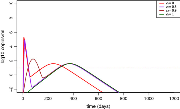
Simulation of viral load dynamics with different drug efficacies ${ϵ}_t$. The other parameters are the same as those in Fig. 5 (color figure online)

Bistability

Table 2 shows that the model has two steady states, ${\mathcal{E}}_0$ and ${\mathcal{E}}_{\mathit{et}}$, when ${\mathcal{R}}_{0b}^c<{\mathcal{R}}_{0b}<1$, ${\mathcal{R}}_{0w}<1$ and ${\psi }^{\prime }(0)<-m$. Although it is challenging to perform a formal mathematical analysis on the stability of the steady state ${\mathcal{E}}_{\mathit{et}}$ in this case, numerical simulation with different initial conditions suggests that ${\mathcal{E}}_{\mathit{et}}$ is locally asymptotically stable (Appendix Fig. 11). Furthermore, using initial conditions of the susceptible and symptomatic infected as an example, we identified the region in which the model converges to the disease-free steady state ${\mathcal{E}}_0$ or the endemic steady state ${\mathcal{E}}_{\mathit{et}}$ (Fig. 6). This shows that the multiscale model exhibits a phenomenon of bistability. With lower levels of initial susceptible and symptomatic infected people, the disease is predicted to die out; when either the number of susceptible or symptomatic infected people exceeds a threshold value, the disease will persist.

Fig. 11.

Model convergence to the endemic steady state ${\mathcal{E}}_{\mathit{et}}$ under differential initial conditions. a The steady state of susceptible S is 565.31, consistent with the calculation $S_0-mI=565.31$; b the steady state of infected I is 2449.68; c the steady state of E is 2140.61, consistent with the calculation ${\theta }_{E}I=2140.61$; d the steady state of R is 422.21, consistent with the calculation ${\theta }_{R}I=422.21$; e the steady state of Z is 8383.85, consistent with the calculation ${\theta }_{Z}I=8383.85$; f the steady state of viral load is 2794.67, consistent with the calculation $V_{+}=f(Z)=f({\theta }_{Z}I)=2794.67$; g the steady state of T is 0.31 cells/ml, consistent with the calculation ${\displaystyle \frac{b}{\kappa V_{+}+d}}=0.31$; h the steady state of infected cells is 0.0035 cells/ml, consistent with the calculation ${\displaystyle \frac{b\kappa V_{+}}{q(\kappa V_{+}+d)}}=0.0035$ (color figure online)

Fig. 6.

Bistability region of the initial susceptible and symptomatic infected in which the model converges to either the steady state ${\mathcal{E}}_0$ or ${\mathcal{E}}_{\mathit{et}}$. The parameters are from Table 3 (color figure online)

Discussion

A large number of mathematical models have been developed to study the dynamics of COVID-19 (for example, see Kucharski et al. 2020; Li et al. 2020; Liu et al. 2020c; Tang et al. 2020; Weitz et al. 2020; Wu et al. 2020a; Zhao and Feng 2020). However, most of the models are focused on the disease transmission at the population level. Several models have been used to study the within-host virus dynamics (Wang et al. 2020; Hernandez-Vargas and Velasco-Hernandez 2020; Gonçalves et al. 2020; Sanche et al. 2020; Goyal et al. 2020). We have not seen any models developed to investigate the coupled dynamics of COVID-19. In this paper, we developed a multiscale model to study the dynamics of COVID-19 at both the within-host and between-host levels. In addition to the assumption that the transmission rate between hosts depends on the viral load within symptomatic infected individuals in some coupled models for other infectious diseases (Tuncer et al. 2016; Childs et al. 2019; Martcheva et al. 2015; Barfield et al. 2018; Nikin-Beers et al. 2018; Dorratoltaj et al. 2017; Numfor et al. 2014; Feng et al. 2015, 2012, 2013; Cen et al. 2014), we introduce a function $\eta (Z)$ into the equation of viral load to represent the inhalation/ingestion rate of the coronavirus from the environment into the human body. This represents the contribution of the environmental reservoirs to the growth of the viral load within individual hosts. Therefore, our model provides a two-way connection between the individual viral kinetics and the population-level disease transmission. In comparison with the above-mentioned coupled models, the transmission rate between hosts in this model was assumed to also depend on the level of infection because a higher level of infection would lead to stronger control measures and consequently reduce the transmission rate. The model is also different from that in Feng et al. (2015, 2013), in which the authors studied a coupled model specifically for an environmentally-driven infectious disease. There was no infection between infected and susceptible individuals considered in that model.

Our analysis approach for the subsystem (i.e., slow or fast subsystem) is similar to that in previous papers including (Yang and Wang 2020). Mathematical analysis of the coupled model is more challenging. We have analyzed the model using the bifurcation theory and a fast-slow analysis, where the latter approach is built upon the time scale separation for the dynamical processes associated with the individual host and the environment and human population. Our detailed analysis on the local and global dynamics of the fast system, the slow system and the coupled system shows that rich dynamics, including both forward and backward bifurcations, emerge with the coupling of the within-host and between-host models. Numerical simulation illustrated the bifurcations (Fig. 1). We have also numerically identified a region in which the disease either persists or dies out (Fig. 6). The emergence of bistability further suggests that the initial populations of susceptible or symptomatic infected can dictate the fate of disease transmission. These bifurcation and bistability results indicate the significance of the proposed coupled modeling approach and highlights the challenges in the prevention and control of the ongoing pandemic.

Both mathematical analysis and the simulation in Fig. 3 suggest that the environmental transmission can contribute to the COVID-19 outbreak and persistence. Potential antiviral treatment can delay the disease outbreak but cannot prevent its emergence. Even when treatment significantly suppresses the viral production within the infected individual, the virus can persist in the host (Fig. 5). This may sound bizarre for a specific individual but it actually makes sense for the conceptual “average” individual considered in the model. If the disease persists at the population level, then the virus will also persist within the average individual due to environmental transmission. Although environmental transmission can contribute to viral persistence within the average host when the disease persists at the population level, it does not mean that environmental transmission plays a dominant role in the disease spread. It depends on the relative magnitude of the transmission terms ${\beta }_{E}SE$, ${\beta }_{I}SI$, and ${\beta }_{Z}SZ$. Most spread of COVID-19 might go through airborne human-to-human transmission (Zhang et al. 2020). Therefore, comprehensive intervention measures such as social distancing and wearing masks, combined with surface disinfection and hand hygiene that can prevent environmental transmission, should be implemented to mitigate the spread of COVID-19 (Pradhan et al. 2020). Our study provides a modeling framework that can be used to evaluate the potential influence of environmental transmission on the disease dynamics.

This is the first attempt to link within-host and between-host dynamics of COVID-19. The validation of multiscale models is usually very challenging as it requires data from all the scales for the same individual or the same region. In this paper, we used the mean viral load of the patients from Hong Kong to represent the within-host dynamics of symptomatic infected individuals and the accumulated cases from Florida to represent the between-host dynamics. Although patients in Florida may have different within-host dynamics, we can use the above as an example to study the mutual impact of the dynamics at one level on the other. Another limitation of our multiscale model is that it assumes individual hosts have the same internal states at a time (i.e., the within-host model is for a conceptual “average” individual). To overcome this limitation, one can couple the within-host and between-host dynamics via the infection age of individuals using the nested modeling approach (Gilchrist and Sasaki 2002; Martcheva et al. 2015), which allows incorporating the staged progression nature of the disease at the population level. There are also some other potential ways to account for the individual within-host heterogeneity in the model, such as adding a subscript i on the within-host variables T, $T^{\ast }$, and V for each individual i or discretizing the population with the level of the viral load as in a recent study (Lin et al. 2021). A more complex model incorporating all the individual heterogeneity will be extremely challenging, if not impossible, for mathematical analysis of the model. Lastly, we used a simple model at each scale to make it analytically more trackable. Immune response was shown to play a significant role in controlling viral replication within infected individuals (Wang et al. 2020; Goyal et al. 2020). The within-host model can be extended to include immune responses but we speculate that it may not have a significant impact on the disease spread at the population level (note that the viral load is suppressed to a very low level in our simulations). A between-host model including more compartments, spatial heterogeneity, stochasticity, and vaccination status would be more realistic to study the disease spread. In a recent work (Lin et al. 2021), Lin et al. used a region-specific model to study the COVID dynamics in a number of populous metropolitan statistical areas in the USA.

To summarize, we have developed a multiscale model to study the interaction between within-host viral replication, the environment, and the disease spread at the population level. The analysis has generated some insights that would not be obtained if the model only considers within-host or between-host dynamics. This work also provides a modeling framework for studying other infectious diseases when the environment can serve as a reservoir of pathogens.

A Proof of Theorem 2

Proof

Consider the Lyapunov function

$$\begin{array}{c}\hfill {\mathcal{L}}^s=\left({\int }_{S^{\ast }}^S,{\displaystyle \frac{x-S^{\ast }}{x}},\mathrm{d},x,+,{\int }_{E^{\ast }}^E,{\displaystyle \frac{x-E^{\ast }}{x}},\mathrm{d},x\right)+c_1{\int }_{I^{\ast }}^I{\displaystyle \frac{x-I^{\ast }}{x}}\mathrm{d}x+c_2{\int }_{Z^{\ast }}^Z{\displaystyle \frac{x-Z^{\ast }}{x}}\mathrm{d}x,\end{array}$$

where $c_1$ and $c_2$ are positive constants to be specified later. It is clear that ${\mathcal{L}}^s\ge 0$ and ${\mathcal{L}}^s=0$ if and only if $(S,E,I,Z)=(S^{\ast },E^{\ast },I^{\ast },Z^{\ast })$. For simplicity, we denote ${\beta }_W^{\ast }=\beta (f(Z^{\ast }),W^{\ast })$ for $W=E,I$ and ${\beta }_Z^{\ast }=\beta (Z^{\ast })$. Differentiating ${\mathcal{L}}^s$ along solutions of system (13) in the main text and using the associated equilibrium equations to simplify, we have

$$\begin{array}{cc}\hfill {\displaystyle \frac{d{\mathcal{L}}^s}{\mathit{dt}}}=& \left({\displaystyle \frac{S-S^{\ast }}{S}},{\displaystyle \frac{\mathit{dS}}{\mathit{dt}}},+,{\displaystyle \frac{E-E^{\ast }}{E}},{\displaystyle \frac{\mathit{dE}}{\mathit{dt}}}\right)+c_1{\displaystyle \frac{I-I^{\ast }}{I}}{\displaystyle \frac{\mathit{dI}}{\mathit{dt}}}+c_2{\displaystyle \frac{Z-Z^{\ast }}{I}}{\displaystyle \frac{\mathit{dZ}}{\mathit{dt}}}\hfill \\ \hfill =& {\displaystyle \frac{S-S^{\ast }}{S}}[({\beta }_E^{\ast }{E}^{\ast }{S}^{\ast }-{\beta }_{E}ES)+({\beta }_I^{\ast }{I}^{\ast }{S}^{\ast }-{\beta }_{I}IS)+({\beta }_Z^{\ast }{Z}^{\ast }{S}^{\ast }-{\beta }_{Z}ZS)]-{\displaystyle \frac{\mu }{S}}{(S-S^{\ast })}^2\hfill \\ \hfill & +{\displaystyle \frac{E-E^{\ast }}{E}}\left[({\beta }_{E}ES-{\beta }_E^{\ast }{E}^{\ast }{S}^{\ast }{\displaystyle \frac{E}{E^{\ast }}}),+,({\beta }_{I}IS-{\beta }_I^{\ast }{I}^{\ast }{S}^{\ast }{\displaystyle \frac{E}{E^{\ast }}}),+,({\beta }_{Z}ZS-{\beta }_Z^{\ast }{Z}^{\ast }{S}^{\ast }{\displaystyle \frac{E}{E^{\ast }}})\right]\hfill \\ \hfill & +c_1{\displaystyle \frac{I-I^{\ast }}{I}}\alpha E^{\ast }\left(\frac{E}{E^{\ast }},-,\frac{I}{I^{\ast }}\right)+c_2{\displaystyle \frac{Z-Z^{\ast }}{Z}}\left({\xi }_E,E,+,{\xi }_I,I,-,{\displaystyle \frac{{\xi }_E{E}^{\ast }+{\xi }^I{I}^{\ast }}{Z^{\ast }}},Z\right).\hfill \end{array}$$

By straightforward calculation, we obtain

$$\begin{array}{cc}\hfill {\displaystyle \frac{d{\mathcal{L}}^s}{\mathit{dt}}}=& -{\displaystyle \frac{\mu }{S}}{(S-S^{\ast })}^2+{\beta }_E^{\ast }{E}^{\ast }{S}^{\ast }\left(1,-,{\displaystyle \frac{S^{\ast }}{S}},-,{\displaystyle \frac{{\beta }_{E}ES}{{\beta }_E^{\ast }{E}^{\ast }{S}^{\ast }}}\right)\hfill \\ \hfill & +\left({\displaystyle \frac{{\beta }_{I}I}{{\beta }_I^{\ast }{I}^{\ast }}}\right)+{\beta }_I^{\ast }{I}^{\ast }{S}^{\ast }\left(1,-,{\displaystyle \frac{S^{\ast }}{S}},-,{\displaystyle \frac{{\beta }_{I}IS}{{\beta }_I^{\ast }{I}^{\ast }{S}^{\ast }}},+,{\displaystyle \frac{{\beta }_{Z}Z}{{\beta }_Z^{\ast }{Z}^{\ast }}}\right)\hfill \\ \hfill & +{\beta }_Z^{\ast }{Z}^{\ast }{S}^{\ast }\left(1,-,{\displaystyle \frac{S^{\ast }}{S}},-,{\displaystyle \frac{{\beta }_{Z}ZS}{{\beta }_Z^{\ast }{Z}^{\ast }{S}^{\ast }}},+,{\displaystyle \frac{{\beta }_{Z}Z}{{{\beta }_Z}^{\ast }{Z}^{\ast }}}\right)+{\beta }_E^{\ast }{E}^{\ast }{S}^{\ast }\left(1,-,{\displaystyle \frac{E}{E^{\ast }}},-,{\displaystyle \frac{{\beta }_{E}S}{{\beta }_E^{\ast }{S}^{\ast }}}\right)\hfill \\ \hfill & \left(+,{\displaystyle \frac{{\beta }_{E}S{E}^{\ast }}{{\beta }_E^{\ast }{S}^{\ast }}}\right)\hfill \\ \hfill & +{\beta }_I^{\ast }{I}^{\ast }{S}^{\ast }\left(1,-,{\displaystyle \frac{E}{E^{\ast }}},-,{\displaystyle \frac{{\beta }_{I}IS{E}^{\ast }}{{\beta }_I^{\ast }{I}^{\ast }{S}^{\ast }E}}\right)\hfill \\ \hfill & +\left({\displaystyle \frac{{\beta }_{I}IS}{{\beta }_I^{\ast }{I}^{\ast }{S}^{\ast }}}\right)+{\beta }_Z^{\ast }{Z}^{\ast }{S}^{\ast }\left(1,-,{\displaystyle \frac{E}{E^{\ast }}},-,{\displaystyle \frac{{\beta }_{Z}ZS{E}^{\ast }}{{\beta }_Z^{\ast }{Z}^{\ast }{S}^{\ast }E}},+,{\displaystyle \frac{{\beta }_{Z}ZS}{{\beta }_Z^{\ast }{Z}^{\ast }{S}^{\ast }}}\right)\hfill \\ \hfill & +c_1\alpha E^{\ast }\left({\displaystyle \frac{E}{E^{\ast }}},-,{\displaystyle \frac{I}{I^{\ast }}},-,{\displaystyle \frac{E{I}^{\ast }}{E^{\ast }I}},+,1\right)+c_2{\xi }_E{E}^{\ast }\left({\displaystyle \frac{E}{E^{\ast }}},-,{\displaystyle \frac{Z}{Z^{\ast }}},-,{\displaystyle \frac{E{Z}^{\ast }}{E^{\ast }Z}},+,1\right)\hfill \\ \hfill & +c_2{\xi }_I{I}^{\ast }\left({\displaystyle \frac{I}{I^{\ast }}},-,{\displaystyle \frac{Z}{Z^{\ast }}},-,{\displaystyle \frac{I{Z}^{\ast }}{I^{\ast }Z}},+,1\right).\hfill \end{array}$$

Hence,

$$\begin{array}{c}\hfill \begin{array}{cc}\hfill {\displaystyle \frac{d{\mathcal{L}}^s}{\mathit{dt}}}& \le {\beta }_E^{\ast }{E}^{\ast }{S}^{\ast }\left({\displaystyle \frac{{\beta }_{E}E}{{\beta }_E^{\ast }{E}^{\ast }}},-,1\right)\left(1,-,{\displaystyle \frac{{\beta }_E^{\ast }}{{\beta }_E}}\right)\hfill \\ \hfill & +{\beta }_I^{\ast }{I}^{\ast }{S}^{\ast }\left[\left({\displaystyle \frac{{\beta }_{I}I}{{\beta }_I^{\ast }{I}^{\ast }}},-,1\right),\left(1,-,{\displaystyle \frac{{\beta }_I^{\ast }}{{\beta }_I}}\right),+,{\displaystyle \frac{I}{I^{\ast }}},-,{\displaystyle \frac{E}{E^{\ast }}},+,ln,{\displaystyle \frac{E}{E^{\ast }}},-,ln,{\displaystyle \frac{I}{I^{\ast }}}\right]\hfill \\ \hfill & +{\beta }_Z^{\ast }{Z}^{\ast }{S}^{\ast }\left[\left({\displaystyle \frac{{\beta }_{Z}Z}{{\beta }_Z^{\ast }{Z}^{\ast }}},-,1\right),\left(1,-,{\displaystyle \frac{{\beta }_Z^{\ast }}{{\beta }_Z}}\right),+,{\displaystyle \frac{Z}{Z^{\ast }}},-,{\displaystyle \frac{E}{E^{\ast }}},+,ln,{\displaystyle \frac{E}{E^{\ast }}},-,ln,{\displaystyle \frac{Z}{Z^{\ast }}}\right]\hfill \\ \hfill & +c_1\alpha E^{\ast }\left({\displaystyle \frac{E}{E^{\ast }}},-,{\displaystyle \frac{I}{I^{\ast }}},-,ln,{\displaystyle \frac{E}{E^{\ast }}},+,ln,{\displaystyle \frac{I}{I^{\ast }}}\right)+c_2{\xi }_E{E}^{\ast }\left({\displaystyle \frac{E}{E^{\ast }}},-,{\displaystyle \frac{Z}{Z^{\ast }}},-,ln,{\displaystyle \frac{E}{E^{\ast }}},+,ln,{\displaystyle \frac{Z}{Z^{\ast }}}\right)\hfill \\ \hfill & +c_2{\xi }_I{I}^{\ast }\left({\displaystyle \frac{I}{I^{\ast }}},-,{\displaystyle \frac{Z}{Z^{\ast }}},-,ln,{\displaystyle \frac{I}{I^{\ast }}},+,ln,{\displaystyle \frac{Z}{Z^{\ast }}}\right).\hfill \\ \hfill \end{array}\end{array}$$

In view of (C1)-(C3) and (H2),

$$\begin{array}{c}\hfill \begin{array}{cc}\hfill {\displaystyle \frac{d{\mathcal{L}}^s}{\mathit{dt}}}& \le (-{\beta }_I^{\ast }{I}^{\ast }{S}^{\ast }-{\beta }_Z^{\ast }{Z}^{\ast }{S}^{\ast }+c_1\alpha E^{\ast }+c_2{\xi }_E{E}^{\ast })\left({\displaystyle \frac{E}{E^{\ast }}},-,ln,{\displaystyle \frac{E}{E^{\ast }}}\right)\hfill \\ \hfill & +({\beta }_I^{\ast }{I}^{\ast }{S}^{\ast }-c_1\alpha E^{\ast }+c_2{\xi }_I{I}^{\ast })\left({\displaystyle \frac{I}{I^{\ast }}},-,ln,{\displaystyle \frac{I}{I^{\ast }}}\right)\hfill \\ \hfill & +({\beta }_Z^{\ast }{Z}^{\ast }{S}^{\ast }-c_2{\xi }_E{E}^{\ast }-c_2{\xi }_I{I}^{\ast })\left({\displaystyle \frac{Z}{Z^{\ast }}},-,ln,{\displaystyle \frac{Z}{Z^{\ast }}}\right).\hfill \end{array}\end{array}$$

Set $c_1={\beta }_I^{\ast }{I}^{\ast }{S}^{\ast }+{\displaystyle \frac{{\xi }_I{I}^{\ast }{\beta }_Z^{\ast }{Z}^{\ast }{S}^{\ast }}{{\beta }_E^{\ast }{E}^{\ast }+{\beta }_I^{\ast }{I}^{\ast }}}$ and $c_2={\displaystyle \frac{{\beta }_Z^{\ast }{Z}^{\ast }{S}^{\ast }}{{\beta }_E^{\ast }{E}^{\ast }+{\beta }_I^{\ast }{I}^{\ast }}}$. As ${\beta }_E^{\ast }{E}^{\ast }+{\beta }_I^{\ast }{I}^{\ast }=\delta Z^{\ast }$, $c_1={\beta }_I^{\ast }{I}^{\ast }{S}^{\ast }+{\xi }_I{I}^{\ast }{\beta }_Z^{\ast }{S}^{\ast }/\delta$ and $c_2={\beta }_Z^{\ast }{S}^{\ast }/\delta$. One can verify that the right-hand side of the above inequality is zero with the chosen $c_1$ and $c_2$. This implies $d{\mathcal{L}}^s/\mathit{dt}\le 0$ in the interior of ${\mathrm{\Omega }}^s$. Furthermore, if $d{\mathcal{L}}^s/\mathit{dt}=0$, then

$$\begin{array}{c}\hfill S=S^{\ast },E=k{E}^{\ast },I=k{I}^{\ast },Z=k{Z}^{\ast }\end{array}$$

for some positive constant k. Substituting this relationship into the first two equations of system (13) in the main text leads to

$$\begin{array}{c}\hfill \mathrm{\Lambda }-(\alpha +\mu )k{E}^{\ast }-\mu S^{\ast }=0,\end{array}$$

which implies $k=1$. Therefore, the only invariant set on which $d{\mathcal{L}}^s/\mathit{dt}=0$ contains the singleton ${\mathcal{E}}_e^s=\{S^{\ast },E^{\ast },I^{\ast },R^{\ast },Z^{\ast }\}$. It follows from the LaSalle Invariant Principle that ${\mathcal{E}}_e$ is globally asymptotically stable in the interior of ${\mathrm{\Omega }}^s$ when ${\mathcal{R}}_0>1$. Consequently, ${\mathcal{E}}_e$ is also unique in the interior of ${\mathrm{\Omega }}^s$. $\square$

B Appendix Figures

See Figs. 7, 8, 9, 10 and 11.

References

- Barfield M, Martcheva M, Tuncer N, Holt RD. Backward bifurcation and oscillations in a nested immuno-eco-epidemiological model. J Biol Dyn. 2018;12(1):51–88. doi: 10.1080/17513758.2017.1401676. [DOI] [PubMed] [Google Scholar]
- Cen X, Feng Z, Zhao Y. Emerging disease dynamics in a model coupling within-host and between-host systems. J Theor Biol. 2014;361:141–151. doi: 10.1016/j.jtbi.2014.07.030. [DOI] [PubMed] [Google Scholar]
- Chan JF-W, Yuan S, Kok K-H, To KK-W, Chu H, Yang J, Xing F, Liu J, Yip CC-Y, Poon RW-S, Tsoi H-W, Lo SK-F, Chan K-H, Poon VK-M, Chan W-M, Ip JD, Cai J-P, Cheng VC-C, Chen H, Hui CK-M, Yuen K-Y. A familial cluster of pneumonia associated with the 2019 novel coronavirus indicating person-to-person transmission: a study of a family cluster. Lancet. 2020;395(10223):514–523. doi: 10.1016/S0140-6736(20)30154-9. [DOI] [PMC free article] [PubMed] [Google Scholar]
- Chen TM, Rui J, Wang QP, Zhao ZY, Cui JA, Yin L (2020) A mathematical model for simulating the phase-based transmissibility of a novel coronavirus. Infect Dis Poverty 9(1) [DOI] [PMC free article] [PubMed]
- Childs LM, El Moustaid F, Gajewski Z, Kadelka S, Nikin-Beers R, Smith JW, Jr, Walker M, Johnson LR. Linked within-host and between-host models and data for infectious diseases: a systematic review. PeerJ. 2019;7:e7057. doi: 10.7717/peerj.7057. [DOI] [PMC free article] [PubMed] [Google Scholar]
- Dorratoltaj N, Nikin-Beers R, Ciupe SM, Eubank SG, Abbas KM. Multi-scale immunoepidemiological modeling of within-host and between-host hiv dynamics: systematic review of mathematical models. PeerJ. 2017;5:e3877. doi: 10.7717/peerj.3877. [DOI] [PMC free article] [PubMed] [Google Scholar]
- Feng Z, Cen X, Zhao Y, Velasco-Hernandez JX. Coupled within-host and between-host dynamics and evolution of virulence. Math Biosci. 2015;270:204–212. doi: 10.1016/j.mbs.2015.02.012. [DOI] [PubMed] [Google Scholar]
- Feng Z, Velasco-Hernandez J, Tapia-Santos B. A mathematical model for coupling within-host and between-host dynamics in an environmentally-driven infectious disease. Math Biosci. 2013;241(1):49–55. doi: 10.1016/j.mbs.2012.09.004. [DOI] [PubMed] [Google Scholar]
- Feng Z, Velasco-Hernandez J, Tapia-Santos B, Leite MCA. A model for coupling within-host and between-host dynamics in an infectious disease. Nonlinear Dyn. 2012;68(3):401–411. doi: 10.1007/s11071-011-0291-0. [DOI] [Google Scholar]
- Gao D, Ruan S. An SIS patch model with variable transmission coefficients. Math Biosci. 2011;232(2):110–115. doi: 10.1016/j.mbs.2011.05.001. [DOI] [PubMed] [Google Scholar]
- Geller C, Varbanov M, Duval RE. Human coronaviruses: insights into environmental resistance and its influence on the development of new antiseptic strategies. Viruses. 2012;4(11):3044–3068. doi: 10.3390/v4113044. [DOI] [PMC free article] [PubMed] [Google Scholar]
- Gilchrist MA, Sasaki A. Modeling host-parasite coevolution: a nested approach based on mechanistic models. J Theor Biol. 2002;218(3):289–308. doi: 10.1006/jtbi.2002.3076. [DOI] [PubMed] [Google Scholar]
- Gonçalves A, Bertrand J, Ke R, Comets E, De Lamballerie X, Malvy D, Pizzorno A, Terrier O, Rosa Calatrava M, Mentré F, et al. Timing of antiviral treatment initiation is critical to reduce sars-cov-2 viral load. CPT: Pharmacometrics Syst Pharmacol. 2020;9(9):509–514. doi: 10.1002/psp4.12543. [DOI] [PMC free article] [PubMed] [Google Scholar]
- Goyal A, Cardozo-Ojeda EF, Schiffer JT (2020) Potency and timing of antiviral therapy as determinants of duration of SARS-CoV-2 shedding and intensity of inflammatory response. Sci Adv 6(47):eabc7112 [DOI] [PMC free article] [PubMed]
- Greenhalgh T, Jimenez JL, Prather KA, Tufekci Z, Fisman D, Schooley R. Ten scientific reasons in support of airborne transmission of sars-cov-2. The Lancet. 2021;397(10285):1603–1605. doi: 10.1016/S0140-6736(21)00869-2. [DOI] [PMC free article] [PubMed] [Google Scholar]
- He S, Tang S, Rong L. A discrete stochastic model of the COVID-19 outbreak: Forecast and control. Math Biosci Eng. 2020;17(4):2792–2804. doi: 10.3934/mbe.2020153. [DOI] [PubMed] [Google Scholar]
- He X, Lau EHY, Wu P, Deng X, Wang J, Hao X, Lau YC, Wong JY, Guan Y, Tan X, Mo X, Chen Y, Liao B, Chen W, Hu F, Zhang Q, Zhong M, Wu Y, Zhao L, Zhang F, Cowling BJ, Li F, Leung GM. Temporal dynamics in viral shedding and transmissibility of COVID-19. Nat Med. 2020;26(5):672–675. doi: 10.1038/s41591-020-0869-5. [DOI] [PubMed] [Google Scholar]
- Hellewell J, Abbott S, Gimma A, Bosse NI, Jarvis CI, Russell TW, Munday JD, Kucharski AJ, Edmunds WJ, Funk S, Eggo RM, Sun F, Flasche S, Quilty BJ, Davies N, Liu Y, Clifford S, Klepac P, Jit M, Diamond C, Gibbs H, van Zandvoort K. Feasibility of controlling COVID-19 outbreaks by isolation of cases and contacts. Lancet Global Health. 2020;8(4):e488–e496. doi: 10.1016/S2214-109X(20)30074-7. [DOI] [PMC free article] [PubMed] [Google Scholar]
- Hernandez-Vargas EA, Velasco-Hernandez JX. In-host mathematical modelling of COVID-19 in humans. Annu Rev Control. 2020;50:448–456. doi: 10.1016/j.arcontrol.2020.09.006. [DOI] [PMC free article] [PubMed] [Google Scholar]
- Jiang X, Rayner S, Luo M-H. Does SARS-CoV-2 has a longer incubation period than SARS and MERS? J Med Virol. 2020;92(5):476–478. doi: 10.1002/jmv.25708. [DOI] [PMC free article] [PubMed] [Google Scholar]
- Ki M. Epidemiologic characteristics of early cases with 2019 novel coronavirus (2019-nCoV) disease in korea. Epidemiol Health. 2020;42:e2020007. doi: 10.4178/epih.e2020007. [DOI] [PMC free article] [PubMed] [Google Scholar]
- Kucharski AJ, Russell TW, Diamond C, Liu Y, Edmunds J, Funk S, Eggo RM, Sun F, Jit M, Munday JD, Davies N, Gimma A, van Zandvoort K, Gibbs H, Hellewell J, Jarvis CI, Clifford S, Quilty BJ, Bosse NI, Abbott S, Klepac P, Flasche S. Early dynamics of transmission and control of COVID-19: a mathematical modelling study. Lancet Infect Dis. 2020;20(5):553–558. doi: 10.1016/S1473-3099(20)30144-4. [DOI] [PMC free article] [PubMed] [Google Scholar]
- Lessler J, Reich NG, Brookmeyer R, Perl TM, Nelson KE, Cummings DA. Incubation periods of acute respiratory viral infections: a systematic review. Lancet Infect Dis. 2009;9(5):291–300. doi: 10.1016/S1473-3099(09)70069-6. [DOI] [PMC free article] [PubMed] [Google Scholar]
- Leung C. The difference in the incubation period of 2019 novel coronavirus (SARS-CoV-2) infection between travelers to hubei and nontravelers: The need for a longer quarantine period. Infect Control Hosp Epidemiol. 2020;41(5):594–596. doi: 10.1017/ice.2020.81. [DOI] [PMC free article] [PubMed] [Google Scholar]
- Li R, Pei S, Chen B, Song Y, Zhang T, Yang W, Shaman J. Substantial undocumented infection facilitates the rapid dissemination of novel coronavirus (SARS-CoV-2) Science. 2020;368(6490):489–493. doi: 10.1126/science.abb3221. [DOI] [PMC free article] [PubMed] [Google Scholar]
- Lin YT, Neumann J, Miller EF, Posner RG, Mallela A, Safta C, Ray J, Thakur G, Chinthavali S, Hlavacek WS. Daily forecasting of regional epidemics of coronavirus disease with bayesian uncertainty quantification, united states. Emerg Infect Dis. 2021;27(3):767–778. doi: 10.3201/eid2703.203364. [DOI] [PMC free article] [PubMed] [Google Scholar]
- Liu PY, He S, Rong LB, Tang SY (2020a) The effect of control measures on COVID-19 transmission in Italy: comparison with Guangdong province in china. Infect Dis Poverty 9(1) [DOI] [PMC free article] [PubMed]
- Liu Y, Yan L-M, Wan L, Xiang T-X, Le A, Liu J-M, Peiris M, Poon LLM, Zhang W (2020b) Viral dynamics in mild and severe cases of COVID-19. Lancet Infect Dis 20(6):656–657 [DOI] [PMC free article] [PubMed]
- Liu Z, Magal P, Seydi O, Webb G (2020c) A COVID-19 epidemic model with latency period. Infect Dis Model 5:323–337 [DOI] [PMC free article] [PubMed]
- Martcheva M, Tuncer N, St Mary C. Coupling within-host and between-host infectious diseases models. Biomath. 2015;42:1510091. [Google Scholar]
- Musa SS, Wang X, Zhao S, Li S, Hussaini N, Wang W, He D (2022) The heterogeneous severity of COVID-19 in African countries: a modeling approach. Bull Math Biol 84(3):1–16 [DOI] [PMC free article] [PubMed]
- Ngonghala CN, Iboi EA, Gumel AB. Could masks curtail the post-lockdown resurgence of covid-19 in the us? Math Biosci. 2020;329:108452. doi: 10.1016/j.mbs.2020.108452. [DOI] [PMC free article] [PubMed] [Google Scholar]
- Nikin-Beers R, Blackwood JC, Childs LM, Ciupe SM. Unraveling within-host signatures of dengue infection at the population level. J Theor Biol. 2018;446:79–86. doi: 10.1016/j.jtbi.2018.03.004. [DOI] [PubMed] [Google Scholar]
- Numfor E, Bhattacharya S, Lenhart S, Martcheva M. Optimal control in coupled within-host and between-host models. Math Model Natural Phenomena. 2014;9(4):171–203. doi: 10.1051/mmnp/20149411. [DOI] [Google Scholar]
- Olabode D, Culp J, Fisher A, Tower A, Hull-Nye D, Wang X (2021) Deterministic and stochastic models for the epidemic dynamics of COVID-19 in Wuhan, China. Math Biosci Eng 18(1):950–967 [DOI] [PubMed]
- Pradhan D, Biswasroy P, Naik PK, Ghosh G, Rath G. A review of current interventions for COVID-19 prevention. Arch Med Res. 2020;51(5):363–374. doi: 10.1016/j.arcmed.2020.04.020. [DOI] [PMC free article] [PubMed] [Google Scholar]
- Salle JPL (1976) The stability of dynamical systems. Society for Industrial and Applied Mathematics
- Sanche S, Lin YT, Xu C, Romero-Severson E, Hengartner N, Ke R. High contagiousness and rapid spread of severe acute respiratory syndrome coronavirus 2. Emerg Infect Dis. 2020;26(7):1470–1477. doi: 10.3201/eid2607.200282. [DOI] [PMC free article] [PubMed] [Google Scholar]
- Sanders JM, Monogue ML, Jodlowski TZ, Cutrell JB. Pharmacologic treatments for coronavirus disease 2019 (COVID-19): a review. JAMA. 2020;323(18):1824–1836. doi: 10.1001/jama.2020.6019. [DOI] [PubMed] [Google Scholar]
- Smith HL, Leenheer PD. Virus dynamics: a global analysis. SIAM J Appl Math. 2003;63(4):1313–1327. doi: 10.1137/S0036139902406905. [DOI] [Google Scholar]
- Spencer JA, Shutt DP, Moser SK, Clegg H, Wearing HJ,Mukundan H, Manore CA (2020) Epidemiological parameter review and comparative dynamics of influenza, respiratory syncytial virus, rhinovirus, human coronavirus, and adenovirus
- Tang B, Wang X, Li Q, Bragazzi NL, Tang S, Xiao Y, Wu J. Estimation of the transmission risk of the 2019-ncov and its implication for public health interventions. J Clin Med. 2020;9(2):462. doi: 10.3390/jcm9020462. [DOI] [PMC free article] [PubMed] [Google Scholar]
- Thieme HR. Persistence under relaxed point-dissipativity (with application to an endemic model) SIAM J Math Anal. 1993;24(2):407–435. doi: 10.1137/0524026. [DOI] [Google Scholar]
- To KK-W, Tsang OT-Y, Leung W-S, Tam AR, Wu T-C, Lung DC, Yip CC-Y, Cai J-P, Chan JM-C, Chik TS-H, Lau DP-L, Choi CY-C, Chen L-L, Chan W-M, Chan K-H, Ip JD, Ng AC-K, Poon RW-S, Luo C-T, Cheng VC-C, Chan JF-W, Hung IF-N, Chen Z, Chen H, Yuen K-Y. Temporal profiles of viral load in posterior oropharyngeal saliva samples and serum antibody responses during infection by SARS-CoV-2: an observational cohort study. Lancet Infect Dis. 2020;20(5):565–574. doi: 10.1016/S1473-3099(20)30196-1. [DOI] [PMC free article] [PubMed] [Google Scholar]
- Tuncer N, Gulbudak H, Cannataro VL, Martcheva M. Structural and practical identifiability issues of immuno-epidemiological vector-host models with application to rift valley fever. Bull Math Biol. 2016;78(9):1796–1827. doi: 10.1007/s11538-016-0200-2. [DOI] [PubMed] [Google Scholar]
- van den Driessche P, Watmough J. Reproduction numbers and sub-threshold endemic equilibria for compartmental models of disease transmission. Math Biosci. 2002;180(1–2):29–48. doi: 10.1016/S0025-5564(02)00108-6. [DOI] [PubMed] [Google Scholar]
- van Doremalen N, Bushmaker T, Morris DH, Holbrook MG, Gamble A, Williamson BN, Tamin A, Harcourt JL, Thornburg NJ, Gerber SI, Lloyd-Smith JO, de Wit E, Munster VJ. Aerosol and surface stability of SARS-CoV-2 as compared with SARS-CoV-1. NEJM. 2020;382(16):1564–1567. doi: 10.1056/NEJMc2004973. [DOI] [PMC free article] [PubMed] [Google Scholar]
- Wang S, Pan Y, Wang Q, Miao H, Brown AN, Rong L. Modeling the viral dynamics of SARS-CoV-2 infection. Math Biosci. 2020;328:108438. doi: 10.1016/j.mbs.2020.108438. [DOI] [PMC free article] [PubMed] [Google Scholar]
- Weitz JS, Beckett SJ, Coenen AR, Demory D, Dominguez-Mirazo M, Dushoff J, Leung C-Y, Li G, Măgălie A, Park SW, Rodriguez-Gonzalez R, Shivam S, Zhao CY. Modeling shield immunity to reduce COVID-19 epidemic spread. Nat Med. 2020;26(6):849–854. doi: 10.1038/s41591-020-0895-3. [DOI] [PMC free article] [PubMed] [Google Scholar]
- Wu JT, Leung K, Bushman M, Kishore N, Niehus R, de Salazar PM, Cowling BJ, Lipsitch M, Leung GM (2020a) Estimating clinical severity of COVID-19 from the transmission dynamics in Wuhan, China. Nat Med 26(4):506–510 [DOI] [PMC free article] [PubMed]
- Wu JT, Leung K, Leung GM (2020b) Nowcasting and forecasting the potential domestic and international spread of the 2019-nCoV outbreak originating in Wuhan, China: a modelling study. Lancet 395(10225):689–697 [DOI] [PMC free article] [PubMed]
- Xue L, Jing S, Miller JC, Sun W, Li H, Estrada-Franco JG, Hyman JM, Zhu H (2020) A data-driven network model for the emerging covid-19 epidemics in Wuhan, Toronto and Italy. Math Biosci, p 108391 [DOI] [PMC free article] [PubMed]
- Yang C, Wang J. A mathematical model for the novel coronavirus epidemic in Wuhan, China. Math Biosci Eng. 2020;17(3):2708–2724. doi: 10.3934/mbe.2020148. [DOI] [PMC free article] [PubMed] [Google Scholar]
- Yeo C, Kaushal S, Yeo D. Enteric involvement of coronaviruses: is faecal–oral transmission of SARS-CoV-2 possible? Lancet Gastroenterol Hepatol. 2020;5(4):335–337. doi: 10.1016/S2468-1253(20)30048-0. [DOI] [PMC free article] [PubMed] [Google Scholar]
- Zhang J, Wang S, Xue Y. Fecal specimen diagnosis 2019 novel coronavirus–infected pneumonia. J Med Virol. 2020;92(6):680–682. doi: 10.1002/jmv.25742. [DOI] [PMC free article] [PubMed] [Google Scholar]
- Zhang R, Li Y, Zhang AL, Wang Y, Molina MJ. Identifying airborne transmission as the dominant route for the spread of covid-19. Proc Natl Acad Sci. 2020;117(26):14857–14863. doi: 10.1073/pnas.2009637117. [DOI] [PMC free article] [PubMed] [Google Scholar]
- Zhao H, Feng Z. Staggered release policies for covid-19 control: costs and benefits of relaxing restrictions by age and risk. Math Biosci. 2020;326:108405. doi: 10.1016/j.mbs.2020.108405. [DOI] [PMC free article] [PubMed] [Google Scholar]
- Zhu N, Zhang D, Wang W, Li X, Yang B, Song J, Zhao X, Huang B, Shi W, Lu R, Niu P, Zhan F, Ma X, Wang D, Xu W, Wu G, Gao GF, Tan W. A novel coronavirus from patients with pneumonia in China, 2019. NEJM. 2020;382(8):727–733. doi: 10.1056/NEJMoa2001017. [DOI] [PMC free article] [PubMed] [Google Scholar]