Immission levels and identification of sulfur dioxide sources in La Oroya city, Peruvian Andes

Abstract

La Oroya is a city in the Peruvian Andes that has suffered a serious deterioration in its air quality, especially due to the high rate of sulfur dioxide (SO₂) emissions, which underlines the importance of knowing its sources of contamination and variation over the years. In this sense, this study aimed to evaluate the immission levels and determine the sources of SO₂ contamination in La Oroya. This analysis was performed using the hourly concentration data of SO₂, and meteorological variables (wind speed and direction), which were analyzed for a period of three years (2018–2020). Graphs of time series, wind and pollutant roses, bivariate polar graphs, clustering k-means, nonparametric statistical tests, and the application of the conditional bivariate probability function were performed to analyze the data and identify the emission sources. The mean concentration of SO₂ was 264.2 μg m⁻³ for the study period, where 55.66 and 2.37% of the evaluated days exceeded the guideline values recommended by the World Health Organization and the Peruvian Environmental Quality Standard for air for 24 h, respectively. The results showed a defined pattern for the daily and monthly variations, with peaks in the morning hours (0900–1000 h LT) and at the end of the year (December), respectively. The main sources of SO₂ emissions identified were light and heavy vehicles that travel through the Central Highway, the La Oroya Metallurgical Complex, the transit of vehicles within the city, and the diesel–electric locomotives that provide cargo transportation services and tourism passenger transportation. The article attempts to contribute to the development of adequate air quality management policies.

Introduction

Exposure to air pollution represents a potential risk to human health, which has caused 300,000 deaths a year only in the Americas, an area where nine out of ten people breathe polluted air (CEPAL, 2020). Air pollution originates from natural and anthropogenic sources, the latter being the largest emitter of atmospheric pollutants (Lang et al., 2016; Yang et al., 2016).

Sulfur dioxide (SO₂) is a criteria pollutant that, when emitted in large quantities into the atmosphere, not only pollutes water and soil through the generation of acid rain (Sudalma-Purwanto et al., 2015; Mosquera et al., 2018; Sagan et al., 2018; García et al., 2013) but also affects human health, harming the respiratory system and altering lung function (Kim et al., 2018; Yang et al., 2016).

Different studies have shown that short periods of exposure to SO₂ (5–10 min) decrease lung function and increase respiratory symptoms in adults with asthma and children, the latter being the most vulnerable, due to their higher inhalation rate per unit of body mass (WHO, 2021; Pal, 2018). The study of SO₂ is of great importance because it is a precursor to other air pollutants, such as PM_2.5, where the SO₄⁻² is part of its composition (García et al., 2013; Lang et al., 2016).

Among the anthropogenic sources of SO₂ are mineral smelters, combustion processes in the vehicle fleet, electric power generation plants, and industrial processes (Bari et al., 2020; Carn et al., 2007; Mosquera et al., 2018; Orellano et al., 2021; Sagan et al., 2018). Muñoz (2020) and Carn et al. (2007) reported that, in the processes of smelters and refineries, significant amounts of SO₂ are released; an example is the extraction of copper from chalcopyrite (CuFeS₂), which in its processing can release up to 2 tons of SO₂ per ton of copper produced. Also, González et al. (2017) found that motorized vehicles in the city of Manizales in Colombia that use gasoline, diesel, and natural gas emit 26 t yr⁻¹ of SO_x, while industrial activity (metallurgy, manufacturing, and food production) generates 113.5 t yr⁻¹ of SO_x; as a consequence, these are considered important sources of SO₂ emissions.

La Oroya is considered one of the cities with the highest level of pollution worldwide, caused mainly by high concentrations of SO₂ (Arellano, 2019; Muñoz, 2020; Sagan et al., 2018). The city is located in central Peru, whose geomorphology is characterized by steep mountains that induce the formation of thermal inversions, which avoids the dispersion of atmospheric pollutants, favoring the increase of pollution levels in the city (Spieler, 2010). One of the economic activities that deteriorated the air quality of this city was the processing of minerals in the La Oroya Metallurgical Complex (CMLO by its acronym in Spanish), which is made up of a set of smelters and refineries, that transform polymetallic minerals into different metals and by-products, releasing considerable amounts of SO₂ (Plasencia & Cabrera 2009).

SO₂ has been monitored for three decades in La Oroya city. Neuman (2016), in the year 2000, found that the concentration levels of SO₂ registered were almost twice the safe value established by the WHO. On the other hand, the General Directorate of Environmental Health and Food Safety of Peru (DIGESA by its acronym in Spanish) has monitored concentrations of SO₂ in the city since 1999, obtaining that from 2009 to 2012 (years that coincide with the cessation of operations from the metallurgical complex), concentrations were below the Environmental Quality Standard for Air (ECA by its acronym in Spanish) of Peru (DIGESA, 2013). It should be noted that in 2012 the CMLO partially reactivated its operations; despite the increase in SO₂ concentration levels, it remained below the ECA. Similarly, the Peruvian Environmental Assessment and Enforcement Agency (OEFA by its acronym in Spanish) monitors SO₂ levels in La Oroya city; thus, in 2017 concentrations of SO₂ were reported to exceed the ECA value (250 μg m⁻³) for 24 h (OEFA, 2017). The aforementioned institutions also identified some emission sources of SO₂, such as the traffic of heavy and light vehicles, and sporadic emissions from the combustion of stoves and ovens of some establishments’ chimneys (DIGESA, 2013; OEFA, 2017).

The air pollutants concentrations are strongly influenced by transport, chemical transformations, and dry–wet deposition (Bartnicki et al., 2018; De Simone et al., 2014). To evaluate these variations, air quality models are used, which are carried out to estimate the distribution of pollutants released into the atmosphere (Demirarslan & Zeybek, 2021). Numerous approaches for mathematical modeling of air quality can be found in the scientific literature, one of these being the receptor model. This model uses statistical techniques to estimate the amount of emissions at local and long distances. Receptor models are often used to identify, characterize, and monitor the distribution of sources of air pollutants (Demirarslan & Zeybek, 2021; Hopke, 2016; Uria-Tellaetxe & Carslaw, 2014).

Among these models, we have the bivariate polar graphs, the k-means clustering, and the conditional bivariate probability function (Demirarslan & Zeybek, 2021), which were implemented in the openair package of the R statistical software, designed for atmospheric data analysis (Carslaw, 2021; Uria-Tellaetxe & Carslaw, 2014). Likewise, the polar annulus analysis allows the evaluation of the variation of the contributions from a specific source as a function of the wind direction and time (Yeganeh et al., 2021). The use of distribution graphs with two or more variables is highly reliable for determining and interpreting the sources of air pollution in a particular area (Hui et al., 2021; Jain et al., 2020; Wei et al., 2020). Recent studies have used the receptor models mentioned above to identify sources of air pollution (Hama et al., 2020; Jorquera & Villalobos, 2020; Prabhu et al., 2020). Hama et al. (2020) used bivariate polar plots and k-means clustering in the Delhi region, India, to identify local sources of PM_2.5 and PM₁₀, finding that road transport and domestic heating were the main sources of pollution. Jorquera and Villalobos (2020) employed k-means clustering to identify the main sources of PM_2.5 and PM₁₀ pollution in three urban areas of Chile, with particular meteorological characteristics and diverse sources of pollution. The study found vehicular traffic, residential wood burning, and windblown dust from the nearby desert environment as the main sources of these pollutants. Prabhu et al. (2020) used the conditional bivariate probability function in the Doon Valley, in the foothills of the Himalayas, to identify local sources of black carbon; the study found that local biomass burning activities for heating and cooking are the main sources of black carbon emissions. Furthermore, Yeganeh et al. (2021) employed polar annulus analysis to visualize the temporal aspects of black carbon concentrations at a spatial scale by wind direction. Due to the aforementioned, these graphs are very useful because they allow the observation of the behavior of pollutants based on wind direction and speed (Ali-Taleshi et al., 2021; Nguyen et al., 2022). Similarly, a comparison of pollutant time series data is essential because it reveals information on contributions from local sources and meteorological conditions (Eunhwa-Woogon et al., 2016).

Therefore, due to the problems that La Oroya has been facing concerning SO₂ (Caycho, 2018; Muñoz, 2020) and the absence of research to date that has identified sources of SO₂ in cities with a complex topography and variable meteorological conditions (Demirarslan & Zeybek, 2021; Hama et al., 2020), it is pertinent to develop air quality management plans. For this reason, the present study aims to identify emission sources and evaluate SO₂ immission levels in La Oroya city through receptor models (bivariate polar plots, the k-means clustering, and the conditional bivariate probability function) during the 2018–2020 period. This research could be a useful tool in air quality management since it will provide valuable information for the formulation of strategies in favor of the local air quality improvement.

Materials and methods

Study area

La Oroya city is located in the Mantaro river basin, Yauli Province, Junín Department, Peru, between geographical coordinates 11° 30' and 12° 00' south latitude and between 75° 30' and 76° 00' west longitude, occupying a total area of 388.42 km² of the Peruvian territory (Caycho, 2018; INGEMMET, 2021). It has an approximate population of 13,595 inhabitants (INEI, 2021), and presents a varied rugged topography with slopes between 2 and 6% in the upper area and 1 to 10% in the lower area (Ureta, 2013). The city is characterized by having a cold and dry climate, with rainfall that can reach up to 800 mm, and is surrounded by mountainous regions, a typical morphological characteristic of the Peruvian Andes (CONAM, 2006). Owing to its geographical and strategic position, it is a forced path for land transport by road and rail, due to its location along both sides of the Central Highway of Peru (Plasencia & Cabrera 2009). Figure 1 presents the study area map and the air quality monitoring station location.

Fig. 1.

Map of the study area and location of the monitoring station

SO₂ concentration data and meteorological parameters

The hourly SO₂ concentration data for the 2018–2020 period was collected from the only air quality monitoring station managed by the OEFA, which is part of the National Air Quality Surveillance Network (OEFA, 2016; OEFA, 2018a). The station is located on the roof of the House of Culture of the Provincial Municipality of Yauli (OEFA, 2021). This station has a Thermo model 43i automatic analyzer and a Campbell model CR1000 automatic meteorological station. The first one uses ultraviolet fluorescence method analysis for the quantification of SO₂ concentrations (MINAM, 2019a), while the second measures meteorological variables, such as wind speed (WS) and wind direction (WD) (OEFA, 2016; OEFA, 2018a).

The analysis method to determine the pollutant concentration, the criteria for the establishment of the monitoring station, and the reliability of the recorded data were carried out following the guidelines defined in the National Air Quality Monitoring Protocols of the years 2005 and 2019 (DIGESA, 2005a; MINAM, 2019a). Figure 1 shows the location of the monitoring station in the study area, and Table 1 presents its general description.

Table 1.

General description of the air quality monitoring station

Code	Location	Latitude	Longitude
CA-CC-01	Comandante Zarate street, block N ° 1—La Oroya, on the roof of the house of culture of the Yauli Provincial Municipality. approximately 700 m from the La Oroya metallurgical complex	11°31′12.44"S	75°54′1.18"O

The station registers hourly SO₂ concentration data continuously; then, these data are validated and published by the same institution (OEFA, 2021). In that sense, due to the easy access, continuous recording, robustness, and reliability of the data, the present research used these station’s data from the 2018–2020 period, to accomplish the stated objectives.

Although using a single monitoring station may limit the air quality monitoring of the entire study area (Jiang et al., 2021), it is necessary to mention that La Oroya has only been studied for its deterioration of air quality caused by the CMLO. Due to this, it was decided to implement a continuous air quality monitoring station following the guidelines of the European Union Commission Directive 2015/1480, which defines the number of monitoring stations based on the number of inhabitants within a city (EU, 2015; OEFA, 2016). However, evaluating the air quality of La Oroya from other perspectives could open the possibility of expanding the monitoring network in the case that more potential sources of pollution are found, which is the main objective of this study.

Methods

Time series

The temporal variation of a pollutant allows to identify the time when the minimum or maximum concentrations occur. Likewise, it shows the behavior pattern, which helps identify the days or months when the concentrations tend to increase or decrease and infer possible sources of contamination (Agustine et al., 2017; Althuwaynee et al., 2020).

In order to study the temporal variation, four-timescale graphs (hour-day, hourly, weekly, and monthly) were made. To compare the concentrations of SO₂ with both the Environmental Quality Standard for Air (ECA) and the guideline value from the World Health Organization (WHO) a time series graph with daily averages was plotted, using the timeVariation and timePlot functions from the R software version 4.0.3 openair package, respectively (R Core Team, 2021).

Wind rose and pollutant rose

A wind rose shows the frequency distribution of the wind direction and speed in different intervals as well as its predominance and maximum value, respectively, within a time interval (Agustine et al., 2017). On the contrary, the pollutant rose applies the same logic but substitutes the wind speed for another set of data, for instance the concentration of a pollutant (Carslaw, 2021; Puentes, 2019). For the elaboration of the wind rose and pollutants rose, hourly records of wind direction, wind speed, and hourly concentrations of SO₂ were used. The windRose and pollutionRose functions of the openair package of R software version 4.0.3 (R Core Team, 2021), were used to obtain the graphs mentioned above, respectively.

Bivariate polar plot

Bivariate polar plots are useful tools for the identification of potential emission sources of an atmospheric pollutant, through a graphical analysis (Carslaw & Ropkins, 2012; Habeebullah, 2013; Rojano et al., 2018). These plots are presented in polar coordinates, which show the variation of a pollutant concentration together with the speed and direction of the wind, allowing the identification of possible emission sources and their dispersion directions, as well as the dependence of the pollutant concentration on the wind speed (Khan et al., 2016). To identify possible SO₂ emission sources in La Oroya city, bivariate polar plots were developed using hourly records of wind direction, wind speed, and hourly SO₂ concentrations. The bivariate polar plots were obtained using the polarPlot function of the openair R software package (Carslaw, 2021). To facilitate the diagram interpretation, this function uses the generalized additive model (gam) for smoothing, which is carried out using the mgcv package (Carlaw, 2021; Carslaw & Beevers, 2013).

K-means clustering of bivariate polar plot

Although bivariate polar plots provide helpful information based only on a graphical analysis determined by the direction and wind speed ranges, they have several limitations in subsequent analyses, since they do not allow the characterization of the different ranges of pollutant concentrations (Carslaw & Beevers, 2013), limitations that the k-means grouping can overcome (Carslaw, 2021). K-means clustering is a method in which similar characteristics of the bivariate polar plot can be identified, selected, and grouped, to improve the understanding of the characteristics of potential sources (Althuwaynee et al., 2020; Carslaw & Beevers, 2013). This grouping was carried out using the polar Cluster function of the openair R package. It is a function that applies grouping techniques to the surfaces generated by the polarPlot; thus, it helps to identify potential characteristics for a more detailed analysis of SO₂ sources (Carslaw, 2021).

Nonparametric statistical tests

The nonparametric statistical tests Kruskal–Wallis and U of Mann–Whitney were applied, with a significance level of 5%, to identify significant differences between the clusters formed by the k-means analysis. The first test reveals the significant differences between the defined groups by comparing the medians of the SO₂ concentration (Chávez, 2020). The second test was used post hoc to compare the pairing of each group, where a Bonferroni adjustment was necessary to increase the level of significance required (Boso et al., 2019; Dinno, 2015). The analyses of both tests were carried out with the kruskal.test and pairwise.wilcox.test functions of the statistical software R version 4.0.3, respectively (R Core Team, 2021).

Conditional bivariate probability function

The conditional probability function (CPF) is used to identify pollution sources and estimates the probability come from a defined wind direction (Δθ) (Begum et al., 2010). In addition, conventional CPF estimates the probability of a measured concentration exceeding a fixed threshold. The CPF is mathematically defined as (Uria-Tellaetxe & Carslaw, 2014):

$$CP{F}_{\mathrm{\Delta }\theta }=\frac{m_{\mathrm{\Delta }\theta |C\ge x}}{n_{\mathrm{\Delta }\theta }}$$

where m_∆Ɵ is the number of samples in the wind sector Δθ whose concentration C is greater than or equal to the reference value x, and n_∆Ɵ is the total number of samples in the wind sector Δθ.

On the other hand, the conditional bivariate probability function (CBPF) couples the CPF with the wind speed, being this the third parameter, subject to be replaced by another variable that allows the distinction between the types of sources based on dispersion (Carslaw & Beevers, 2013). This function designates the analyzed contaminant concentration to the cells of direction and wind speed ranges, providing greater reliability than conventional methods that only establish the concentrations of pollutants in the sectors determined by the wind direction (Carslaw, 2021). The incorporation of a third variable provides more information regarding the type of source of interest. In that sense, the CBPF is appropriate for the identification of pollution sources in areas characterized by a high complexity of emission sources (Althuwaynee et al., 2020; Uria-Tellaetxe & Carslaw, 2014). The CBPF can be defined as (Carslaw, 2021):

$$CBP{F}_{\mathrm{\Delta }\theta }=\frac{m_{\mathrm{\Delta }\theta ,\mathrm{\Delta }\mu |C\ge x}}{n_{\mathrm{\Delta }\theta ,\mathrm{\Delta }\mu }}$$

where m_∆Ɵ,∆µ is the number of samples in the wind sector Δθ with a wind speed interval Δu, whose concentration C is greater than a reference value x, and n_∆Ɵ,∆µ is the total number of samples in that wind speed–direction interval. The CBPF was used to validate the most significant sources of SO₂. The implementation of this technique was carried out using the polarPlot function with the “cpf” statistic from the openair package of the R software version 4.0.3 (R Core Team, 2021).

Results and discussions

The descriptive statistics of SO₂ in the study area are presented in Table 2. It is observed that the hourly concentrations of SO₂ ranged from 6.5 to 3,315.1 μg m⁻³, 7.9 to 2,964.8 μg m⁻³ and 4.5 to 2,894.2 μg m⁻³, with averages of 78.74 μg m⁻³, 57.45 μg m⁻³ and 65.41 μg m⁻³ for the years 2018, 2019 and 2020, respectively. These variations may be associated with the influence that meteorological parameters (Althuwaynee et al., 2020) and terrain topography have over the behavior of air pollutants (Alván, 2010; Arrieta, 2016).

Table 2.

Descriptive statistics of SO₂ levels in La Oroya city

	2018	2019	2020
Minimum	6.5	7.9	4.5
Maximum	3,315.10	2,964.80	2,894.20
1. Quartile	11.3	10.7	10.7
3. Quartile	35.6	27.5	16.5
Mean	78.74 ± 2.27	57.45 ± 1.58	65.41 ± 2.33
Median	13.9	14.7	12.3
Stdev	207.1	144.3	211.1
Skewness	5.9	6.1	6.4
Kurtosis	48.6	55.4	52
Missing data %	4.9	5.3	6.7

On the other hand, it is observed that the asymmetry and kurtosis values varied in the range of 5.9 to 6.4 and 48.66 to 55.4, respectively. These results demonstrate the asymmetric behavior of the SO₂ concentration. According to O'Leary et al. (2016), Ottosen and Kumar (2019), an asymmetric behavior of the data occurs possibly due to the influence of outliers above the 75 percentile.

Box-and-whisker plots

Due to the significant presence of outliers, the box-and-whisker diagram is presented without drawing the outliers in order to achieve a better graphical representation (Fig. 2) (R core team, 2021). In this research, outliers were not eliminated, because their presence is indicative of the diversity and a high number of SO₂ pollution sources in La Oroya city (Caycho, 2018; Estevan et al., 2019, 2020; Plasencia & Cabrera, 2009). Likewise, it is common that in atmospheric sciences, data sets with outliers are presented, so their exclusion, systematic elimination, or transformation could hide important atmospheric environmental processes and lead to incorrect conclusions that can difficult the decision making, or even lead to the adoption of inadequate management programs (Benhadi-Marín, 2018; O'Leary et al., 2016). Finally, it is essential to mention that the hourly data concentrations of SO₂ are validated by OEFA, and the monitoring station is subject to periodic evaluations carried out by this institution (OEFA, 2021).

Fig. 2.

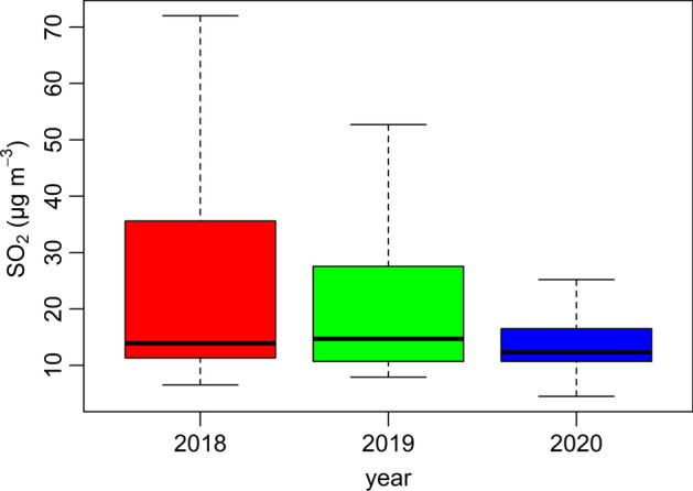
Box-and-whisker plot of SO₂ concentrations

The graph shows that the interquartile range is comparatively higher in 2018 and lower in 2020. Therefore, it is inferred that there was higher variability of SO₂ concentrations in 2018 and intermediate variability in the year 2020.

The temporal variation in four timescales (hour-day, hourly, weekly, and monthly) of SO₂ concentrations during 2018, 2019, and 2020 (Carslaw, 2021) is shown in Fig. 3. It is observed that during the day there is a peak between 0900 and 1000 h local time (LT) with an average concentration of 264.2 μg m^-3 that exceeds the guideline values, of 40 μg m⁻³ and 250 μg m⁻³, established by WHO and the national ECA, respectively. At a monthly level, SO₂ concentrations do not follow a homogeneous trend in the three years period, but they do register a minimum average value in June (26.4 μg m⁻³) and a maximum average in December (126.1 μg m⁻³). At the weekly level, the variation was more notable, without defined patterns.

Fig. 3.

Temporal variation of SO₂ concentrations

Sagan et al. (2018) and Zarauz et al. (2010) also recorded variations in SO₂ concentrations in La Oroya and found that the main factors influencing the dispersion of pollutants were the oscillation of the planetary boundary layer, topography, thermal inversions, and changes in wind direction and speed. This is due to the fact that the mountainous areas of the Peruvian Andes form a natural physical barrier for wind circulation and make it impossible for the polluted air to be removed from the area. In addition, the dry climate in these places increases the frequency of thermal inversions (García et al., 2013). The complex topography of La Oroya city determines the speed and direction of airflows, hampering the circulation during the contaminant transport process, thus preventing dispersion (Cheng et al., 2022; Caycho, 2018; Ibañez et al., 2021; Sagan et al., 2018; Arrieta, 2016). This factor also influences the amount of solar radiation received by the earth's surface throughout the day, which generates atmospheric pressure differences that produce air mass movements (Cheng et al., 2013, 2022; Zardi & Whiteman, 2013), and give rise to mountain–valley wind systems, which are characteristic of the city (Mamani, 2013; Vidal & Pérez, 2017).

Bei et al. (2018) found that the atmospheric contaminants formed in the afternoon are transported by the valley winds from an urban area to the mountains, being stored in the latter, while at night, due to the action of mountain winds, they are put back to the urban area, causing greater pollution. Cao et al. (2020) reported that the mountain–valley winds were stronger on sunny days than on cloudy days in the city of Sichuan, China; they also mentioned that these systems originate the transport of pollutants between the city and the mountains, increasing the level of air pollution in the city. The phenomenon described above has also been evidenced in the city of La Oroya due to its topographical characteristics, as reported by Mamani (2013), who states that the valley–mountain wind system of the city influences the wind flows and therefore the dispersion of SO₂ concentrations.

On the other hand, due to its geographical, meteorological, and topographical characteristics, the city of La Oroya is exposed to temperature inversions that prevent adequate diffusion of gaseous pollutants, settling in the city for long periods of time (Alván, 2010; Cerdestav & Barandiarán, 2002; Mendiola et al., 2017; Tello, 2014). The planetary boundary layer of the city is between 700 and 800 m; however, this vertical structure varies during the day and night, and between wet and dry periods.

Below the boundary layer, the thermal inversion phenomenon occurs, which originates and varies according to the aforementioned periods, presenting a greater negative impact on air quality during the dry period. During this period, the thermal inversion generally becomes frequent at the end of the day between 1800 h LT and 1900 h LT, until 0900 h LT and 1000 h LT the next day, so there are high levels of gas concentration in the mornings, while in the afternoon the intensity of the winds increases and the atmosphere becomes unstable, which favors the dispersion of gases and reduces the impact on air quality (CONAM, 2004; CONAM, 2006; Córdova, 2008). According to Giovannini et al. (2020), this phenomenon in mountainous regions can even extend to periods ranging from several days to several weeks, since the low visibility factor of the sky limits the penetration of solar radiation in the valleys, and the night drainage winds favor the accumulation of cold air at low levels. The temperature decrease during the mornings generates thermal inversion and, in combination with the low humidity of the environment, causes contaminants to be trapped in the bottom and prolong its duration (García et al., 2013).

The hourly peak in the mornings is possibly related to the greater intensity of vehicular traffic on the Central Highway, where heavy and light vehicles circulate, and to which the emissions from fugitive sources from the CMLO would be added (Alarcón, 2016; Integral Consulting, 2005; Red Muqui, 2020; OEFA, 2018b,c–d). In Peru, it has been reported that 90 and 58.1% of cargo and passenger transport vehicles, respectively, use petroleum (diesel), a fossil fuel with high concentrations of sulfur and an important source of SO₂ (MINEM, 2017; Fei et al., 2018). The patterns identified between vehicle fleet and SO₂ concentrations are explained because SO₂ is generated as a product of the incomplete combustion of sulfurized hydrocarbon fuels (USEPA, 2020).

It is important to mention that the proximity of the monitoring station to the main highway may have favored the recording of peak concentrations from heavy traffic at the hourly level (Mohtar et al., 2018). In their study, De Souza et al. (2019) reported a maximum peak of high concentrations of SO₂ at 1100 h LT and related it to the increase of vehicular traffic in Campo Grande, Brazil, in 2016. The influence of transport on SO₂ concentration was also reported by Yang et al. (2018), as they determined that transportation contributed to 10% of China's total emissions during 2002.

In addition, the industrial sector has been recorded as a large contributor to SO₂ emissions, according to various studies. For example, Min et al. (2021) found that industrial processes and industrial combustion in Sichuan, China were the main contributors of SO₂ emissions with 46% and 29%, respectively, in 2017. Akyuz and Kaynak (2019) reported that in Turkey, the energy sector was the main source of SO₂ emission because 70% of the total electricity was generated with a 50% share of coal-fired power plants (CPP) using sub-bituminous and lignite coal as fuel, which contain a large amount of sulfur. Li et al. (2017) calculated China’s emissions inventory for the year 2010 by sectors and found that the industrial sector contributed 57.39% to total SO₂ emissions.

However, in Peru, according to the Lima-Callao Air Quality Management Diagnosis of 2019, mobile sources were the main contributors of SO₂ emissions with a contribution of 54.79%, while point and area sources only contributed 33.02 and 12.18%, respectively. Within the point sources, the industrial activity of zinc refining was the main contributor to SO₂ emissions (MINAM, 2019b). On the other hand, although in La Oroya, the main contribution of SO₂ emissions (380,075 t-SO₂ yr⁻¹) in 2005 came from the CMLO's metal smelting and refining processes (representing 99% of total SO₂ emissions) (CONAM, 2004; CONAM, 2006; DIGESA, 2005b), fugitive sources from it have also been responsible for most of the local impacts, especially in La Oroya Antigua and La Oroya Nueva (DIGESA, 2005b; Integral Consulting, 2005).

Finally, as described in the previous paragraph, in Lima-Callao and La Oroya, SO₂ contributions from metal refining activities have been considerable, but their contribution has been decreasing. In the case of La Oroya, these emissions have been decreasing with the partial cessation of the CMLO's activities. Therefore, currently other sources, mainly mobile sources, could equal or exceed the contribution of the polymetallic smelter and refining.

The reduction of SO₂ emissions from the CMLO affects the immission levels of La Oroya. Morales (2018) evaluated the concentrations of SO₂ during the operation and shutdown of the CMLO, and found that the concentrations of SO₂ were higher than 2,500 μg m⁻³ in the year 2008, while, after the operations stopped, the SO₂ immission level was below the minimum value established by DIGESA to consider La Oroya city in a state of alert (arithmetic average of 24 h > 500 μg m⁻³ of SO₂).

Comparison with ECA and WHO guideline values.

The temporal variation of SO₂ in La Oroya with a daily resolution (24-h average) is presented in Fig. 4. The daily levels exceeded the WHO guideline value (40 μg m⁻³) on 610 days, representing 55.66% of the days of the study period (2018–2020). The national ECA for SO₂ (250 μg m⁻³) was exceeded during 26 days, representing 2.37% of days of the study period. The days with the highest concentrations that exceeded the national regulations were recorded at the end of 2020, which was possibly associated with the partial lifting of health restrictions in the framework of the COVID-19 pandemic (Rojas et al., 2021; Toro et al., 2021; Morales et al., 2021). Several studies worldwide identified an increase in air pollutant concentrations as the pandemic restrictive measures were lifted (Anil & Alagha, 2021; He et al., 2021; Wang et al., 2021). According to the WHO, high levels of exposure to this gas can affect the respiratory system, lung function, cause eye irritation and aggravate asthma and chronic bronchitis; it also increases hospital admissions for heart disease and mortality rates (WHO, 2006; WHO, 2021).

Fig. 4.

Daily temporal variation of SO₂ in La Oroya city

Source identification of SO₂ by wind rose and pollutant rose

The wind rose for the study period is shown in Fig. 5. The predominant direction of the wind is from the west (W) throughout the four seasons. Likewise, variable directions are evident in all seasons. Zarauz (2011) observed similar wind direction behavior at the CMLO main chimney, located approximately 700 m SE from the monitoring station. The mean wind speed ranged from 1.177 m s⁻¹ (autumn) to 1.4197 m s⁻¹ (spring). The lower wind speeds recorded in March, April, and May, added to the presence of thermal inversions, cause stagnant air masses and a consequent increase of SO₂ concentrations in La Oroya (Espinoza & Alderete, 2021; Sagan et al., 2018; Silva et al., 2017).

Fig. 5.

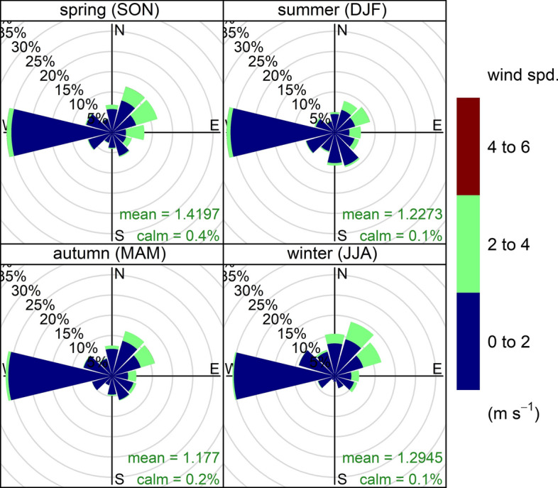
Wind rose by seasons of the year during the 2018–2020 period

The inverse relationship between wind speed and SO₂ concentration is evidenced in the pollutant rose (Fig. 6). At lower wind speeds (0 to 0.8 m s⁻¹), there is a higher average concentration (93.732 μg m⁻³) of the pollutant, while at higher wind speeds (1.7 to 5.6 m s⁻¹), there is a lower average concentration (32.166 μg m⁻³) of SO₂. Mid-concentrations of the pollutant were recorded in the speed ranges from 0.8 to 1.1 m s⁻¹ (72.739 μg m⁻³) and 1.1 to 1.7 m s⁻¹ (64.593 μg m⁻³). Other studies also reported that at lower wind speeds, higher concentrations of pollutants are recorded, due to its low dispersion (Sooktawee et al., 2020; Althuwaynee et al., 2020; Perišić, 2020; Jindamanee et al., 2020; Mohtar et al., 2018; Jang et al., 2017).

Fig. 6.

Pollutant roses for SO₂ hourly concentrations by wind speed intervals during the 2018–2020 period

When analyzing the yearly seasonal correlation between wind speed and SO₂ concentration, it was determined that during the summer, the correlation was higher (|− 0.10|≤ r ≤|− 0.48|), followed by spring (|− 0.12| ≤ r ≤|− 0.33|), autumn (|− 0.04|≤ r ≤|− 0.34|), and winter (|− 0.02|≤ r ≤|− 0.09|). These correlations improve when analyzing the data set by month. It was observed that all the correlations between both parameters are negative, which confirmed the inverse relationship between wind speed and SO₂ concentrations, these being stronger in the summer and spring seasons. Dandotiya et al. (2020) and Chao et al. (2021) also found an inverse correlation (r = − 0.38 and r = − 0.34, respectively) between both parameters. Li and Xie (2016) explained that the inverse relationship between wind speeds and SO₂ concentrations is because lower wind speeds do not promote the diffusion of the pollutant, which results in higher monthly concentrations of SO₂, while, in conditions with higher wind speeds, the diffusion of SO₂ is favored, so monthly concentration ​​are lower.

The inverse relationship found in La Oroya could also be related to the proximity between the emission source and the monitoring station, due to its direct impact on the readings of the monitoring equipment, but this would not limit the registration of lower concentrations coming from possible distant sources (Althuwaynee et al., 2021; Moufarrej et al., 2020; Sooktawee et al., 2020).

Pollution peaks within the range of 150 to 3,315.1 μg m⁻³ occurred more frequently at low velocities and in the south (S), southeast (SE), and east (E) directions, where one of Peru's main highways, the CMLO and the railroad with the Huancayo–La Oroya–Lima route are located. Between 4,000 and 4,300 vehicles per day travel along the Central Highway, including heavy and light vehicles, most of which use petroleum (diesel) as their main fuel (Alarcón, 2016; MINEM, 2017). The CMLO is classified as one of the largest refineries in Peru and has been declared a major source of SO₂. However, in recent years it has been operating at a limited capacity and a non-constant period (Requejo, 2020; TFA, 2021; MINEM, 2020; Red Muqui, 2020). Trains with diesel–electric locomotives run on the railroad, mainly for freight transportation and, to a lesser extent, for tourist passenger service with scheduled departures along the Huancayo–La Oroya–Lima route (OSITRAN, 2020; FVCA, 2006).

Additionally, high concentrations were observed at low wind speeds coming from the west (W) of the monitoring station, which may be associated with vehicle traffic within La Oroya city (Concepción & Rodríguez, 2014). In addition, to the west–south–west (WSW) and approximately one kilometer away, there is a critical point of vehicular congestion due to the convergence of three highways from Cerro de Pasco, Huancayo, and Lima, where light and heavy vehicles circulate (CONAM, 2004). Finally, to the west (W) and southwest (SW) there is the railway that connects the cities of Cerro de Pasco, Junín, La Oroya, and Lima, where freight trains from important mining centers frequently pass through, being the main transported products: copper concentrate, zinc concentrate, lead concentrate, and industrial sulfuric acid (OSITRAN, 2020; MINCUL, 2019). The aforementioned sources explain the high concentrations recorded in the west (W) direction.

Given the presence of mobile sources in all wind directions and their significant contribution to SO₂ concentrations in La Oroya, to complement the study, SO₂ emissions from this source were estimated for the 2018–2020 period. The calculation of emissions followed the updated Tier 1 methodology described in the Air pollutant emission inventory guidebook of the European Environment Agency (EEA, 2021). Vehicle fleet data estimated by the Ministry of Transport and Communications (MTC by its acronym in Spanish) (MTC, 2021) were used and it was considered that the fuels used by these vehicles were Gasohol, diesel, and LPG (OSINERGMIN, 2021). It was estimated that for the years 2018, 2019, and 2020, SO₂ emissions were 9,852, 10,103, and 8,704 t-SO₂ yr⁻¹, respectively. These values ​​far exceeded the emissions from mobile sources of SO₂ reported in the latest emissions inventory of La Oroya (83 t-SO₂ yr⁻¹) (DIGESA, 2005b), which clearly shows the progressive growth of the vehicle fleet throughout the years (MTC, 2021), bringing with it, the increase in the concentration of SO₂ in the city of La Oroya. These SO₂ emissions lead to an increase in the concentration of the pollutant. In the study conducted by Yang et al. (2016) in China, it was found that the emission of 10,000 tons of SO₂ increases the environmental concentration of the pollutant by 0.463 μg m⁻³. This estimation confirms the importance of La Oroya’s vehicle fleet in the contributions of SO₂ concentrations in recent years. The high rate of emission by this source can be alarming. A deeper study and more detailed analysis of the sulfur dioxide emissions in this city or the department of Junín and its contribution to the concentrations of sulfur dioxide can be a relevant subject for future research.

On the other hand, the contamination range from 0 to 50 μg m⁻³ of SO₂ occurs in all wind directions and wind speeds, which can be attributed to the sources close to the monitoring point (Sooktawee et al., 2020), in addition to those already mentioned. The OEFA (2018e, f, g, h, i), during the execution of its air quality surveillance plan, observed sporadic emissions from chimneys at 30 m from the monitoring point, which were generated as a result of the combustion of fuels in ovens, restaurant kitchens, and other establishments. According to the air quality baseline diagnosis reported in 2004, these emissions would contribute minimally to SO₂ concentrations, since the use of oil and kerosene in some establishments, mainly bakeries and restaurants, emits low amounts of SO₂ (CONAM, 2004).

Source identification of SO₂ by bivariate polar plots and k-means clustering

The bivariate polar graphs of SO₂ concentrations by seasons for the 2018–2020 period in La Oroya city are shown in Fig. 7. The color scale in the figure shows the SO₂ concentration in μg m⁻³, and the radial scale represents the wind speed in m s⁻¹ which increases radially from the center of the diagram. High concentrations of SO₂ are observed mainly in the southwest (SW), south (S), and southeast (SE) directions throughout the four seasons of the year, being particularly high during the spring and summer of the southern hemisphere. The sources of pollution that might contribute to the high concentrations of SO₂ in these directions could be the Central Highway, the CMLO, and the railways through which diesel freight and passenger trains travel (Requejo, 2020; TFA, 2021; MINEM, 2020; Red Muqui, 2020). In the air quality surveillance monitoring reports from the years 2016, 2017, and 2018, the presence of emissions from the CMLO, from the automotive fleet (cars, trucks, and trains), and to a lesser extent from some commercial and service establishments (restaurants and bakeries) was evidenced (OEFA 2016, OEFA, 2017, OEFA, 2018g, h–i).

Fig. 7.

Bivariate polar graphs from the concentrations of SO₂, WS, and WD

Likewise, a possible source of contamination in the SW direction, with less contribution than the previous ones and that is remarkable during the summer and autumn seasons in the wind speed range from 2 to 3 m s⁻¹, would also be associated with the transit of cargo and passenger trains that follow the Huancayo–La Oroya–Lima and Unishp (Cerro de Pasco)–La Oroya–Lima routes, that circulate along the railway located at a distance of approximately 500 m from the monitoring station (OSITRAN, 2020; FVCA, 2006). Finally, the graphs also showed that in the rest of the wind directions, SO₂ concentrations are minimal, which could indicate that there is no significant source of pollution in those directions.

The k-means clustering of the bivariate polar graphs for the SO₂ concentrations is shown in Fig. 8. The diagram was divided into 3 clusters, to characterize the SO₂ emission sources in the Oroya city. The red (CL1), blue (CL2), and green (CL3) clusters represent high, medium, and low concentrations of SO₂, respectively. The clusters with the highest concentration in the SE, S and SW directions are mainly influenced by vehicular emissions from the Central Highway, produced by the oil or diesel incomplete combustion process, where sulfur as part of the composition of these fuels is burned and emitted in the form of SO₂ (Khobragade et al., 2018). On the other hand, CMLO emissions might also contribute to the high concentrations in the red cluster (CL1). The CMLO mainly processes copper, lead, and zinc concentrate, which contain high concentrations of sulfur, an element that is released in high amounts as SO₂ during the heating process of the concentrate (Carn et al., 2007; Della et al., 2017; Fioletov et al., 2016). Zhang et al. (2021) identified metal smelters as one of the important sources of SO₂ in China, contributing to 20% of total SO₂ emissions in 2012. Mohtar et al. (2018) reported that the main source of SO₂ in power plants and industrial facilities is the burning of fossil fuels. Finally, the trains that travel on the railroad also contribute to SO₂ emissions since they use diesel–electric locomotives (OSITRAN, 2020). The high emissions of SO₂ generated during the incomplete combustion of diesel or gasoline could be reduced by lowering the sulfur content in these fuels (Miranda et al., 2016; Mohtar et al., 2018; Rodríguez, 2017).

Fig. 8.

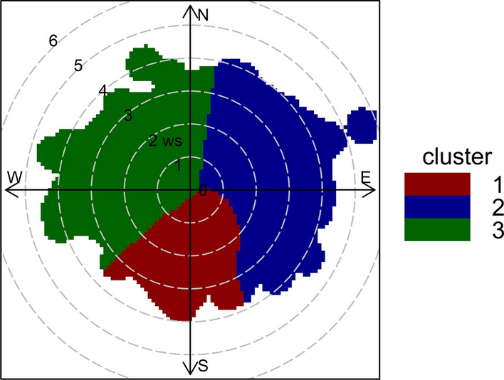
Clustering of k-means on the bivariate polar graph

Figure 8 reaffirmed that the highest concentrations of SO₂ come from the SE, S, and SW directions, being associated with three possible sources of contamination such as the traffic of vehicles on the Central Highway, the CMLO, and the trains.

The multiannual temporal variation of SO₂ concentrations for each defined cluster is shown in Fig. 9. Temporal analysis shows average concentrations with a 95% confidence interval (Carslaw, 2021). The cluster with the highest concentration (CL1) reflects the characteristic behavior of vehicular flow in La Oroya city (Alarcón, 2016; Concepción & Rodríguez, 2014). In general, there are two daily peaks, one in the morning and the other in the afternoon, which is related to the traffic congestion caused in those periods (Alarcón, 2016). In addition, the decrease in the concentration of SO₂ is observed during noon, which may be related to the turbulent conditions of the atmosphere at this time, which enhances the dispersion of pollutants (Espinoza & Alderete, 2021; Habeebullah, 2013; Sagan et al., 2018; Zarauz et al., 2010). Likewise, it was identified that the concentrations of SO₂ associated with CL1 were different from those of CL2 and CL3, but, between the latter, there were no significant differences.

Fig. 9.

Multiyear temporal variation of the SO₂ clusters in La Oroya city

Monthly there is a marked and differentiated behavior between the three clusters. The CL2 and CL3 show an almost constant average in all months of the year, which may indicate that the concentrations come from fixed sources, while the monthly variation of CL1 follows a variable behavior in which lower values are evidenced in June and higher in the last months of the year. The characteristic monthly behavior of CL1 could be mainly associated with the development of economic activities, particularly the production, transportation, and processing of minerals. According to records from the Ministry of Energy and Mines (MINEM, by its acronym in Spanish) and the Central Reserve Bank of Peru (BCRP, by its acronym in Spanish), the average production of metals such as Cu, Zn, and Pb in the Junín region for the study period was higher at the end of the year (September, October, November, and December) and less in the middle of the year (April, May, June, and July). The production was exceptionally high at the end of 2020, a period that coincided with the progressive lifting of sanitary restrictions due to COVID-19 (MINEM, 2021; BCRP, 2021; Rojas et al., 2021). In addition, Alarcón (2016) reported that the interprovincial transport service along the Central Highway also followed a defined pattern, registering the highest number of trips at the beginning and the end of the year and the lowest at midyear. In this sense, the processing of the minerals and the number of trips made in trains and vehicles throughout the year would explain the monthly behavior of the cluster that registered the highest concentrations of SO₂.

Table 3 presents the results of the Kruskal–Wallis and Mann–Whitney U tests for the clusters of SO₂ concentrations. The nonparametric Kruskal–Wallis test identified the existence of differences between the groups formed by the k-means cluster analysis at a significance level of 5% (p < 0.05), which further reinforces the findings. The Mann–Whitney U test identified the group that differs from the other groups formed, through pairwise multiple comparisons (Calazans et al., 2018). The results of the multiple comparison test confirmed that the red cluster (CL1) contributed more to the concentrations of SO₂, which is associated with emissions from heavy and light vehicle traffic, with contributions from the CMLO and with emissions from train traffic. Clusters 2 and 3 also showed significant differences at 5%; however, their average values and behavior are similar, which may indicate predominant emission sources with similarity for both clusters or the absence of important sources in the directions they represent (Al-Harbi et al., 2020). The Mann–Whitney U test proves to be an effective tool for determining significant differences between clusters (Chávez, 2020).

Table 3.

Results of the Kruskal–Wallis and Mann–Whitney U tests in the SO₂ clusters

Cluster	Mean	Chi-squared	df	p-value	Pairwise	Mann–Whitney
CL1	238.0	4823	2	< 2.2e–16	CL1–CL2	< 2e–16
CL2	28.1				CL1–CL3	< 2e–16
CL3	30.6				CL2–CL3	< 2e–16

Source identification of SO₂ by conditional bivariate probability function

Finally, the graphs generated with the CBPF for concentrations of SO₂ are shown in Fig. 10. CBPF plots show relevant hidden information about other pollution sources that are not distinguishable in bivariate polar plots, so their use is appropriate for places with high emission source complexity (Althuwaynee et al., 2020, 2021). A 75th percentile was established to represent the sources with the highest contribution to SO₂ concentrations (Uria-Tellaetxe & Carslaw, 2014). The analysis validated the main sources identified. Thus, significant concentrations of SO₂ (> 75th percentile—25 μg m⁻³) were identified with a probability of occurrence of 90% or more in the SE, S, and SW directions, during the four seasons of the year and throughout the speed range. This is mainly related to the emissions from mobile sources that travel along the Central Highway and the contributions from the CMLO. A greater probability of the occurrence of significant concentrations greater than the 75th percentile was also observed in the spring and summer seasons compared to the autumn and winter seasons, which agrees with the findings from the other methods applied in this study. A higher concentration of SO₂ in the spring and summer seasons, and a lower one in the autumn and winter seasons, could be related to the climatic conditions of the place under study, considering that areas with dry climates such as La Oroya, can contribute to severe haze episodes with high concentrations of SO₂ (CONAM, 2006; García et al., 2013).

Fig. 10.

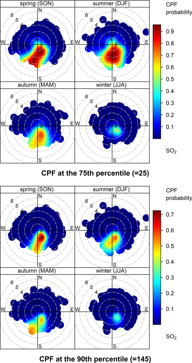
Conditional bivariate probability function at the 75th and 90th percentiles for SO₂ concentrations

The CBPF at the 90th percentile showed similar behavior to the 75th percentile. However, it helped to identify an additional significant source of SO₂ in the south–southwest direction (SSW), whose predominance occurred in March, April, and May and in the spring and summer seasons. That behavior might be associated with the movement of freight and passenger trains at different times of the day, which constitute another of the mobile sources of air quality pollution in La Oroya (DIGESA, 2013).

Conclusions and recommendations

In this study, the immission levels were evaluated and the potential sources of SO₂ emissions were identified from hourly records of SO₂, direction, and wind speed, in La Oroya city. The mean SO₂ concentration for the study period was 264.2 μg m⁻³. Likewise, it was found that the daily average concentrations of this pollutant exceeded the guideline value established by the WHO and the ECA air during 610 and 26 days, respectively. The highest number of days that exceeded these values was recorded in 2020, which coincided with the progressive lifting of sanitary restrictions due to COVID-19 in Peru. The daily variation of the pollutant concentrations presented a daily peak, recorded in the morning hours (0900–1000 h LT), which coincides with the characteristic behavior of the vehicular flow of the study area, added to the complex relief topographical and meteorological conditions of the place. At a monthly level, the highest monthly averages of SO₂ were recorded in December; this was associated with the highest production of minerals and interprovincial passenger transport recorded in this month. The predominant winds were from the West (W) during the four seasons, with an average speed between 1.177 m s⁻¹ (autumn) and 1.4197 m s⁻¹ (spring), as shown in the wind roses. While the analysis with the pollutant roses allowed to determine that at lower wind speeds (0–0.8 m s⁻¹), higher concentrations (93.732 μg m⁻³) of the pollutant occur in the S, SE, and E directions of the monitoring station. The bivariate polar graphs and their subsequent grouping using the k-means algorithm showed that the highest concentrations of SO₂ mainly occur in the S, SE, and SW directions throughout the year, which are mainly influenced by the emissions from the fleet of light and heavy vehicles that travel daily on the Central Highway, possible emissions from the La Oroya Metallurgical Complex and the traffic of diesel–electric locomotives that travel the railways surrounding the city. The analysis using the conditional bivariate probability function with 75th and 90th percentiles made it possible to validate the sources of contamination identified with the other methods used and to estimate the concentrations most influenced by the main sources of contamination. Finally, the need arises to continue working on the development of more advanced models that incorporate other atmospheric and topographic variables, thus allowing more accurate characterization of temporal variations and the influence of these variables on the dispersion of the pollutant.

Author contributions

JAEG was responsible for conceptualization, methodology, formal analysis, writing the original draft, writing, reviewing, and editing, supervision, and resources. MBAM was involved in methodology, writing the original draft, writing, reviewing, and editing, supervision, and resources. JHCC, DLPH, DFVLR, and SJBM had contributed to writing the original draft, writing, reviewing, and editing, visualization, and resources.

Funding

This research did not receive any specific grant from funding agencies in the public, commercial, or not-for-proft sectors.

Data availability

The data that support the findings of this study are available from the corresponding author, upon reasonable request.

Declarations

Conflict of interest

The authors declare that they have no conflict of interest.

Consent for publication

Not applicable.

Ethics approval

Not applicable.

References

- Agustine I, Yulinawati H, Suswantoro E, Gunawan D. Application of open air model (R Package) to analyze air pollution data. Indonesian Journal of Urban and Environmental Technology. 2017;1(1):94–109. doi: 10.25105/urbanenvirotech.v1i1.2430. [DOI] [Google Scholar]
- Akyuz E, Kaynak B. Use of dispersion model and satellite SO2 retrievals for environmental impact assessment of coal-fired power plants. Science of the Total Environment. 2019;689:808–819. doi: 10.1016/j.scitotenv.2019.06.464. [DOI] [PubMed] [Google Scholar]
- Alarcón, F. (2016). La importancia de la Carretera Central. Reporte. Retrieved October 5, 2021, from https://bit.ly/3nTanaB
- Al-Harbi M, Al-majed A, Abahussain A. Spatiotemporal variations and source apportionment of NOx, SO2, and O3 emissions around heavily industrial locality. Environmental Engineering Research. 2020;25(2):147–162. doi: 10.4491/eer.2018.414. [DOI] [Google Scholar]
- Ali-Taleshi MS, Moeinaddini M, Bakhtiari AR, Feiznia S, Squizzato S, Bourliva A. A one-year monitoring of spatiotemporal variations of PM2.5-bound PAHs in Tehran, Iran: source apportionment, local and regional sources origins and source-specific cancer risk assessment. Environmental Pollution. 2021;274:115883. doi: 10.1016/j.envpol.2020.115883. [DOI] [PubMed] [Google Scholar]
- Althuwaynee OF, Balogun AL, Al Madhoun W. Air pollution hazard assessment using decision tree algorithms and bivariate probability cluster polar function: Evaluating inter-correlation clusters of PM10 and other air pollutants. Giscience & Remote Sensing. 2020;57(2):207–226. doi: 10.1080/15481603.2020.1712064. [DOI] [Google Scholar]
- Althuwaynee OF, Pokharel B, Aydda A, Balogun AL, Kim SW, Park HJ. Spatial identification and temporal prediction of air pollution sources using conditional bivariate probability function and time series signature. Journal of Exposure Science and Environmental Epidemiology. 2021;31(4):709–726. doi: 10.1038/s41370-020-00271-8. [DOI] [PubMed] [Google Scholar]
- Alván, N. (2010). Evaluación y diagnóstico de los niveles de dióxido de azufre en la ciudad de La Oroya. Tesis de grado. Universidad Nacional del Callao. Retrieved May 10, 2022, from https://bit.ly/3mCDhuR
- Anil I, Alagha O. The impact of COVID-19 lockdown on the air quality of Eastern Province, Saudi Arabia. Air Quality, Atmosphere & Health. 2021;14(1):117–128. doi: 10.1007/s11869-020-00918-3. [DOI] [PMC free article] [PubMed] [Google Scholar]
- Arellano, R. (2019). El reglamento ambiental minero en la continuidad laboral en la Oroya. Tesis de grado. Universidad Autónoma del Perú. Retrieved October 14, 2021, from https://hdl.handle.net/20.500.13067/687
- Arrieta AJ. Dispersión De Material Particulado (PM10), con interrelación de factores meteorológicos y topográficos. Ingeniería Investigación y Desarrollo. 2016;16(2):43–54. doi: 10.19053/1900771x.v16.n2.2016.5445. [DOI] [Google Scholar]
- Banco Central de Reserva del Perú (BCRP) (2021). Producción de productos mineros según departamentos. Retrieved October 22, 2021, from https://bit.ly/3aIQejX
- Bari MA, Kindzierski WB, Roy P. Identification of ambient SO2 sources in industrial areas in the lower Athabasca oil sands region of Alberta, Canada. Atmospheric Environment. 2020;231:117–505. doi: 10.1016/j.atmosenv.2020.117505. [DOI] [Google Scholar]
- Bartnicki J, Semeena VS, Mazur A, Zwoździak J. Contribution of Poland to atmospheric nitrogen deposition to the Baltic Sea. Water, Air, & Soil Pollution. 2018;229(11):1–22. doi: 10.1007/s11270-018-4009-5. [DOI] [PMC free article] [PubMed] [Google Scholar]
- Begum BA, Biswas SK, Markwitz A, Hopke PK. Identification of sources of fine and coarse particulate matter in Dhaka. Bangladesh. Aerosol and Air Quality Research. 2010;10(4):345–353. doi: 10.4209/aaqr.2009.12.0082. [DOI] [Google Scholar]
- Bei N, Zhao L, Wu J, Li X, Feng T, Li G. Impacts of sea-land and mountain-valley circulations on the air pollution in Beijing-Tianjin-Hebei (BTH): A case study. Environmental Pollution. 2018;234:429–438. doi: 10.1016/j.envpol.2017.11.066. [DOI] [PubMed] [Google Scholar]
- Benhadi-Marín J. A conceptual framework to deal with outliers in ecology. Biodiversity and Conservation. 2018;27(12):3295–3300. doi: 10.1007/s10531-018-1602-2. [DOI] [Google Scholar]
- Boso À, Álvarez B, Oltra C, Hofflinger Á, Vallejos-Romero A, Garrido J. Examining patterns of air quality perception: A cluster analysis for southern Chilean cities. SAGE Open. 2019;9(3):1–11. doi: 10.1177/2158244019863563. [DOI] [Google Scholar]
- Calazans GM, Pinto CC, da Costa EP, Perini AF, Oliveira SC. The use of multivariate statistical methods for optimization of the surface water quality network monitoring in the Paraopeba river basin. Brazil. Environmental Monitoring and Assessment. 2018;190(8):1–17. doi: 10.1007/s10661-018-6873-2. [DOI] [PubMed] [Google Scholar]
- Cao B, Wang X, Ning G, Yuan L, Jiang M, Zhang X, Wang S. Factors influencing the boundary layer height and their relationship with air quality in the Sichuan Basin. China Science of the Total Environment. 2020;727:138584. doi: 10.1016/j.scitotenv.2020.138584. [DOI] [PubMed] [Google Scholar]
- Carn SA, Krueger AJ, Krotkov NA, Yang K, Levelt PF. Sulfur dioxide emissions from Peruvian copper smelters detected by the ozone monitoring instrument. Geophysical Research Letters. 2007 doi: 10.1029/2006GL029020. [DOI] [Google Scholar]
- Carslaw, D.C. (2021). Package “openair”. Tools for the Analysis of Air Pollution Data. Retrieved October 2, 2021, from https://cran.r-project.org/web/packages/openair/openair.pdf
- Carslaw DC, Beevers SD. Characterising and understanding emission sources using bivariate polar plots and k-means clustering. Environmental Modelling & Software. 2013;40:325–329. doi: 10.1016/j.envsoft.2012.09.005. [DOI] [Google Scholar]
- Carslaw DC, Ropkins K. Openair—an R package for air quality data analysis. Environmental Modelling & Software. 2012;27–28:52–61. doi: 10.1016/j.envsoft.2011.09.008. [DOI] [Google Scholar]
- Caycho Bustamante, M. K. (2018). Elaboración de un plan de alerta ambiental preventiva en la calidad de aire (dióxido de azufre y plomo) en la Ciudad de la Oroya. Retrieved October 10, 2021, from http://repositorio.unfv.edu.pe/handle/UNFV/2316
- Cerdestav A.K., & Barandiarán A. (2002). La Oroya no espera. Sociedad Peruana de Derecho Ambiental. Retrieved May 10, 2022, from https://bit.ly/3Q43v6U
- Chao C, Min B. Correlation analysis of atmospheric pollutants and meteorological factors based on environmental big data. International Journal of Contents. 2021;18(1):17–26. doi: 10.5392/IJoC.2022.18.1.017. [DOI] [Google Scholar]
- Chávez E. Incidence of the quarantine due to COVID-19, in the air quality (NO2) of the city of Lima. Rev. del Instituto de Investigación FIGMMG-UNMSM. 2020;23(46):65–71. doi: 10.15381/iigeo.v23i46.18183. [DOI] [Google Scholar]
- Cheng FY, Hsu YC, Lin PL, Lin TH. Investigation of the effects of different land use and land cover patterns on mesoscale meteorological simulations in the Taiwan area. Journal of Applied Meteorology and Climatology. 2013;52(3):570–587. doi: 10.1175/JAMC-D-12-0109.1. [DOI] [Google Scholar]
- Cheng FY, Wang YT, Huang MQ, Lin PL, Lin CH, Lin PH, Wang SH, Tsuang BJ. Boundary Layer Characteristics Over Complex Terrain in Central Taiwan: Observations and Numerical Modeling. Journal of Geophysical Research: Atmospheres. 2022;127(2):e2021JD035726. doi: 10.1029/2021JD035726. [DOI] [Google Scholar]
- Concepción, E., & Rodríguez, J. M. (2014). Informe Nacional de la Calidad del Aire 2013–2014. Retrieved October 27, 2021, from https://bit.ly/3mdRGgC
- Consejo Nacional del Ambiente (CONAM). (2004). Diagnóstico de línea base de calidad del aire de La Oroya. Retrieved October 10, 2021, from https://bit.ly/3MoiJQU
- Consejo Nacional del Ambiente (CONAM). (2006). Plan de Acción para la Mejora de la Calidad del Aire en la Cuenca Atmosférica de La Oroya. Retrieved October 10, 2021, from https://bit.ly/3zeSrhj
- Comisión Económica para América Latina y el Caribe (CEPAL). (2020). Efectos de las cuarentenas y restricciones de actividad relacionadas con el COVID-19 sobre la calidad del aire en las ciudades de América Latina. CEPAL, 1–13. Retrieved October 15, 2021, from https://bit.ly/3NodTVm
- Córdova R. (2008). Evaluación de las concentraciones del plomo, cadmio y arsénico de las deposiciones de material particulado en las áreas libres de las instituciones educativas de nivel inicial y primario en Yauli-La Oroya. Tesis de grado. Universidad Nacional del Centro del Perú. Retrieved May 10, 2022, from http://hdl.handle.net/20.500.12894/216
- Dandotiya B, Harendra K, Jadon N. Ambient Air Quality and meteorological monitoring of gaseous pollutants in urban areas of Gwalior City India. Environmental Claims Journal. 2020;32(3):248–253. doi: 10.1080/10406026.2020.1744854. [DOI] [Google Scholar]
- De Simone F, Gencarelli CN, Hedgecock IM, Pirrone N. Global atmospheric cycle of mercury: A model study on the impact of oxidation mechanisms. Environmental Science and Pollution Research. 2014;21(6):4110–4123. doi: 10.1007/s11356-013-2451-x. [DOI] [PubMed] [Google Scholar]
- De Souza, A., Jan, B., Nawaz, F., Ayub Khan Yousuf Zai, M., Santos de Oliveira, S., Pavao, H. G., Fernandes, W. A., & Amaury de Souza, C. (2019). Temporal variations of SO2 in an urban environment. Discovery, 55(283), 328–339. https://bit.ly/3aKL3A9
- Della L, Micheletti M, Freire M, García B, Piacentini R. SO2 and aerosol evolution over the very clear atmosphere at the argentina andes range sites of San antonio de los cobres and El leoncito. Proceedings. 2017;1(5):197. doi: 10.3390/ecas2017-04153. [DOI] [Google Scholar]
- Demirarslan KO, Zeybek M. Conventional air pollutant source determination using bivariate polar plot in Black Sea, Turkey. Environment, Development and Sustainability. 2021;24(2):2736–2766. doi: 10.1007/s10668-021-01553-3. [DOI] [Google Scholar]
- Dinno A. Nonparametric pairwise multiple comparisons in independent groups using Dunn's test. The Stata Journal. 2015;15(1):292–300. doi: 10.1177/1536867X1501500117. [DOI] [Google Scholar]
- Dirección General de Salud Ambiental e Inocuidad Alimentaria (DIGESA). (2005a). R.D. Nº 1404–2005a-DIGESA: Resolución Directoral que aprueba el Protocolo de Monitoreo de Calidad del Aire y Gestión de Datos. Lima, Perú. Retrieved October 13, 2021, from https://bit.ly/3NR7cuL
- Dirección General de Salud Ambiental e Inocuidad Alimentaria (DIGESA). (2005b). Inventario de emisiones cuenca atmosférica de la ciudad de La Oroya. Retrieved December 10, 2021, from https://bit.ly/3xkOBS8
- Dirección General de Salud Ambiental e Inocuidad Alimentaria (DIGESA). (2013). Informe N° 001810–2013/DEPA/DIGESA. Vigilancia Sanitaria de la Calidad del Aire por el reinicio de las actividades del Complejo Metalúrgico de Doe Run Perú. Retrieved October 13, 2021, from https://bit.ly/3NnQlQs
- Estevan, R., Martínez-Castro, D., Suarez-Salas, L., Moya, A., & Silva, Y. (2020). Mediciones de aerosoles con un fotómetro solar AERONET en el Observatorio de Huancayo, Perú. Boletín científico El Niño, 7(3), 4–11. https://repositorio.igp.gob.pe/handle/20.500.12816/4880
- Estevan R, Martínez-Castro D, Suarez-Salas L, Moya A, Silva Y. First two and a half years of aerosol measurements with an AERONET sunphotometer at the Huancayo Observatory. Peru. Atmospheric Environment: X. 2019;3:100037. doi: 10.1016/j.aeaoa.2019.100037. [DOI] [Google Scholar]
- Eunhwa J, Woogon D, Geehyeong P, Minkyeong K, Eunchul Y. Spatial and temporal variation of urban air pollutants and their concentrations in relation to meteorological conditions at four sites in Busan, South Korea. Atmospheric Pollution Research. 2016;8:89–100. doi: 10.1016/j.apr.2016.07.009. [DOI] [Google Scholar]
- European Environment Agency (EEA). (2021). Air pollutant emission inventory guidebook 2019 – Update Oct. 2021. Retrieved May 10, 2022, from https://bit.ly/3NquGqM
- Fei L, Sungyeon C, Can L, Vitali EF, Chris AM. A new global anthropogenic SO2 emission inventory for the last decade: A mosaic of satellite-derived and bottom-up emissions. Atmospheric Chemistry and Physics. 2018;18(22):16571–16586. doi: 10.5194/acp-18-16571-2018. [DOI] [Google Scholar]
- Ferrovías Central Andina S.A (FVCA). (2006). Reglamento de Acceso a la Infraestructura de la Concesionaria Ferrovías Central Andina S.A. Retrieved October 30, 2021, from https://bit.ly/3mhVqOn
- Fioletov VE, McLinden CA, Krotkov N, Li C, Joiner J, Theys N, Carn S, Moran MD. A global catalogue of large SO2 sources and emissions derived from the Ozone Monitoring Instrument. Atmospheric Chemistry and Physics. 2016;16(18):11497–11519. doi: 10.5194/acp-16-11497-2016. [DOI] [Google Scholar]
- García M, Ramírez H, Ulloa H, García O, Meulenert A, Alcalá J. Concentration of pollutants SO2, NO2 and correlation with H+, SO4-2 and NO3– during wet season in the Metropolitan Zone of Guadalajara, Jalisco, Mexico. Rev Chil Enf Respir. 2013;29:81–88. doi: 10.4067/S0717-73482013000200004. [DOI] [Google Scholar]
- Instituto Geológico, Minero y Metalúrgico (INGEMMET). (2021). Geología del cuadrángulo de La Oroya (hojas 24l1, 24l2, 24l3, 24l4). Instituto Geológico Minero y Metalúrgico. Retrieved October 16, 2021, from https://bit.ly/3NVGl0v
- Giovannini L, Ferrero E, Karl T, Rotach MW, Staquet C, Castelli ST, Zardi D. Atmospheric pollutant dispersion over complex terrain: Challenges and needs for improving air quality measurements and modeling. Atmosphere. 2020;11(6):1–32. doi: 10.3390/atmos11060646. [DOI] [Google Scholar]
- González CM, Gómez CD, Rojas NY, Acevedo H, Aristizábal BH. Relative impact of on-road vehicular and point-source industrial emissions of air pollutants in a medium-sized Andean city. Atmospheric Environment. 2017;152:279–289. doi: 10.1016/j.atmosenv.2016.12.048. [DOI] [Google Scholar]
- Espinoza-Guillen JA, Alderete-Malpartida MB. Caracterización de regiones espacialmente homogéneas de monóxido de carbono en Lima Metropolitana mediante el algoritmo de clustering k-means. Revista Científica: Biotech and Engineering. 2021;1(1):17–28. doi: 10.52248/eb.Vol1Iss01.4. [DOI] [Google Scholar]
- Habeebullah TM. An analysis of air pollution in Makkah - A view point of source identification. EnvironmentAsia. 2013;6(2):11–17. doi: 10.14456/ea.2013.12. [DOI] [Google Scholar]
- Hama SM, Kumar P, Harrison RM, Bloss WJ, Khare M, Mishra S, Namdeo A, Sokhi R, Goodman P, Sharma C. Four-year assessment of ambient particulate matter and trace gases in the Delhi-NCR region of India. Sustainable Cities and Society. 2020;54:102003. doi: 10.1016/j.scs.2019.102003. [DOI] [Google Scholar]
- He C, Song Hong L, Zhang HM, Xin A, Zhou Y, Liu J, Liu N, Yuming S, Tian Y, Ke B, Yanwen Wang L, Yang, Global, continental, and national variation in PM2.5, O3, and NO2 concentrations during the early 2020 COVID-19 lockdown. Atmospheric Pollution Research. 2021;12(3):136–145. doi: 10.1016/j.apr.2021.02.002. [DOI] [PMC free article] [PubMed] [Google Scholar]
- Hopke PK. Review of receptor modeling methods for source apportionment. Journal of the Air & Waste Management Association. 2016;66(3):237–259. doi: 10.1080/10962247.2016.1140693. [DOI] [PubMed] [Google Scholar]
- Hui L, Ma T, Gao Z, Gao J, Wang Z, Xue L, Liu H, Liu J. Characteristics and sources of volatile organic compounds during high ozone episodes: A case study at a site in the eastern Guanzhong Plain. China Chemosphere. 2021;265:129072. doi: 10.1016/j.chemosphere.2020.129072. [DOI] [PubMed] [Google Scholar]
- Ibañez M, Gironás J, Oberli C, Chadwick C, Garreaud RD. Daily and seasonal variation of the surface temperature lapse rate and 0 C isotherm height in the western subtropical Andes. International Journal of Climatology. 2021;41:E980–E999. doi: 10.1002/joc.6743. [DOI] [Google Scholar]
- Integral Consulting. (2005). Modelamiento de dispersión de la calidad del aire para el estudio de riesgos para la salud humana. Complejo metalúrgico La Oroya. Retrieved October 4, 2021, from https://bit.ly/3NYrfri
- Jain S, Sharma SK, Vijayan N, Mandal TK. Seasonal characteristics of aerosols (PM2.5 and PM10) and their source apportionment using PMF: A four year study over Delhi. India. Environmental Pollution. 2020;262:114337. doi: 10.1016/j.envpol.2020.114337. [DOI] [PubMed] [Google Scholar]
- Jang E, Do W, Park G, Kim M, Yoo E. Spatial and temporal variation of urban air pollutants and their concentrations in relation to meteorological conditions at four sites in Busan. South Korea. Atmospheric Pollution Research. 2017;8(1):89–100. doi: 10.1016/j.apr.2016.07.009. [DOI] [Google Scholar]
- Jiang L, He S, Zhou H, Kong H, Wang J, Cui Y, Wang L. Coordination between sulfur dioxide pollution control and rapid economic growth in China: Evidence from satellite observations and spatial econometric models. Structural Change and Economic Dynamics. 2021;57:279–291. doi: 10.1016/j.strueco.2021.04.001. [DOI] [Google Scholar]
- Jindamanee K, Thepanondh S, Aggapongpisit N, Sooktawee S. Source apportionment analysis of volatile organic compounds using positive matrix factorization coupled with conditional bivariate probability function in the industrial areas. EnvironmentAsia. 2020;12(2):31–49. doi: 10.14456/ea.2020.28. [DOI] [Google Scholar]
- Jorquera H, Villalobos AM. Combining cluster analysis of air pollution and meteorological data with receptor model results for ambient PM2.5 and PM10. International Journal of Environmental Research and Public Health. 2020;17(22):8455. doi: 10.3390/ijerph17228455. [DOI] [PMC free article] [PubMed] [Google Scholar]
- Khan MB, Masiol M, Formenton G, Di Gilio A, de Gennaro G, Agostinelli C, Pavoni B. Carbonaceous PM2.5 and secondary organic aerosol across the Veneto region (NE Italy) Science of the Total Environment. 2016;542:172–181. doi: 10.1016/j.scitotenv.2015.10.103. [DOI] [PubMed] [Google Scholar]
- Khobragade R, Einaga H, Jain S, Saravanan G, Labhsetwar N. Sulfur dioxide-tolerant strontium chromate for the catalytic oxidation of diesel particulate matter. Catalysis Science & Technology. 2018;8(6):1712–1721. doi: 10.1039/C7CY02553J. [DOI] [Google Scholar]
- Kim D, Chen Z, Zhou LF, Huang SX. Air pollutants and early origins of respiratory diseases. Chronic Diseases and Translational Medicine. 2018;4(2):75–94. doi: 10.1016/j.cdtm.2018.03.003. [DOI] [PMC free article] [PubMed] [Google Scholar]
- Lang J, Zhou Y, Cheng S, Zhang Y, Dong M, Li S, Wang G, Zhang Y. Unregulated pollutant emissions from on-road vehicles in China, 1999–2014. Science of the Total Environment. 2016;573:974–984. doi: 10.1016/j.scitotenv.2016.08.171. [DOI] [PubMed] [Google Scholar]
- Li M, Liu H, Geng G, Hong C, Liu F, Song Y, Tong D, Zheng B, Cui H, Man H, Zhang Q, He K. Anthropogenic emission inventories in China: A review. National Science Review. 2017;4(6):834–866. doi: 10.1093/nsr/nwx150. [DOI] [Google Scholar]
- Li S, Xie S. Spatial distribution and source analysis of SO2 concentration in Urumqi. International Journal of Hydrogen Energy. 2016;41(35):15899–15908. doi: 10.1016/j.ijhydene.2016.04.142. [DOI] [Google Scholar]
- Mamani, D. (2013). Simulación de la circulación atmosférica a nivel superficial para la cuenca del Río Mantaro usando el modelo atmosférico de mesoescala MM5. Tesis de grado. Universidad Nacional Mayor de San Marcos. Retrieved May 10, 2022, from https://bit.ly/3NFB1il
- Mendiola, A., Aguirre, C., Carpio, C. A., Monroy, V., & Paredes, Y. (2017). Perspectivas de reestructuración del Complejo Metalúrgico de La Oroya mediante un análisis ambiental y económico. In Journal of Chemical Information and Modeling. Retrieved May 10, 2022, from https://hdl.handle.net/20.500.12640/1220
- Min, H., Junhui, C., Yuming, H., Yuang, L., & Qichao, L. (2021). Trends and Source Contribution Characteristics of SO2, NOX, PM10 and PM2.5 Emissions in Sichuan Province from 2013 to 2017. Atmosphere, 12(2), 189. 10.3390/atmos12020189
- Ministerio de Cultura (MINCUL). (2019). Ferrocarril Central del Perú. Retrieved October 9, 2021, from https://bit.ly/3MkIhOV
- Ministerio de Energía y Minas (MINEM). (2017). Guía de Orientación del Uso Eficiente de la Energía y de Diagnóstico Energético. Dirección General de Eficiencia Energética. Retrieved October 9, 2021, from https://bit.ly/3NYhetW
- Ministerio de Energía y Minas (MINEM). (2020). Resolución Directoral N° 0443–2020-MINEM-DGM. Retrieved October 30, 2021, from https://bit.ly/3ayipBO
- Ministerio de Energía y Minas (MINEM). (2021). Producción Minera Anual 2011–2020. Retrieved October 21, 2021, from https://bit.ly/3zjYdOB
- Ministerio de Transportes y Comunicaciones (MTC) (2021). Parque Vehicular Nacional Estimado, según Departamento: 2007–2018. Retrieved May 10, 2022, from https://bit.ly/3mgDm7f
- Ministerio del Ambiente (MINAM). (2019a). Decreto Supremo N° 010–2019a-MINAM. - Decreto Supremo que aprueba el Protocolo Nacional de Monitoreo de la Calidad Ambiental del Aire. Ministerio del Ambiente, República del Perú. Retrieved October 10, 2021, from https://bit.ly/3x9JqU2
- Ministerio del Ambiente (MINAM). (2019b). Diagnóstico de la gestión de la calidad ambiental del aire de Lima y Callao. Retrieved May 10, 2022,from https://bit.ly/3Qf4H7A
- Miranda J, Martínez S, Kenedy J, Figueroa R, Aguirre N. Diagnóstico de contaminación atmosférica por emisiones diésel en la zona metropolitana de San Salvador y Santa Tecla. Entorno. 2016;61:7–16. doi: 10.5377/entorno.v0i61.6125. [DOI] [Google Scholar]
- Mohtar, A. A. A., Latif, M. T., Baharudin, N. H., Ahamad, F., Chung, J. X., Othman, M., & Juneng, L. (2018). Variation of major air pollutants in different seasonal conditions in an urban environment in Malaysia. Geoscience Letters, 5(21), 1-13. 10.1186/s40562-018-0122-y
- Morales, J. (2018). Evaluación de impactos ambientales generados por los gases del proceso de fundición y refinería de metales de la empresa Doe Run Perú S.R.L. en la Provincia Yauli. Tesis de grado. Universidad Nacional Daniel Alcides Carrión. Retrieved May 10, 2022, from https://bit.ly/3zmm7ci
- Morales-Solís K, Ahumada H, Rojas JP, Urdanivia FR, Catalán F, Claramunt T, R.A., Manzano, C.A., & Leiva-Guzmán, M.A. The Effect of COVID-19 lockdowns on the air pollution of urban areas of central and southern chile. Aerosol and Air Quality Research. 2021;21:200677. doi: 10.4209/aaqr.200677. [DOI] [Google Scholar]
- Mosquera, A. P., Duque, C. M., García, M., & Aristizábal, B. H. (2018). Distribución Espacial de Concentraciones de SO2, NOx y O3 en el Aire Ambiente de Manizales. Revista Internacional de Contaminación Ambiental, 34(3), 489–504. 10.20937/RICA.2018.34.03.11
- Moufarrej, L., Courcot, D., & Ledoux, F. (2020). Assessment of the PM2.5 oxidative potential in a coastal industrial city in Northern France: Relationships with chemical composition, local emissions and long range sources. Science of The Total Environment, 748, 141448. 10.1016/j.scitotenv.2020.141448 [DOI] [PubMed]
- Muñoz, C. (2020). Significado de vivir en una ciudad con alta contaminación ambiental en profesionales de salud: foráneos y nativos arraigados en La Oroya - Junín, Perú 2019. Tesis de Doctorado. Universidad Nacional Mayor de San Marcos. Retrieved October 21, 2021, from https://hdl.handle.net/20.500.12672/15617
- Instituto Nacional de Estadística e Informática (INEI). (2021). Población estimada por regiones al 2021. Retrieved October 16, 2021, from https://bit.ly/3xcDBVW
- Neuman P. Toxic Talk and Collective (In)action in a Company Town: The Case of La Oroya, Peru. Social Problems. 2016;63:431–446. doi: 10.1093/socpro/spw010. [DOI] [Google Scholar]
- Nguyen TNT, Vuong QT, Lee SJ, Xiao H, Choi SD. Identification of source areas of polycyclic aromatic hydrocarbons in Ulsan, South Korea, using hybrid receptor models and the conditional bivariate probability function. Environmental Science: Processes & Impacts. 2022;24:140–151. doi: 10.1039/D1EM00320H. [DOI] [PubMed] [Google Scholar]
- O'Leary B, Reiners JJ, Jr, Xu X, Lemke LD. Identification and influence of spatio-temporal outliers in urban air quality measurements. Science of the Total Environment. 2016;573:55–65. doi: 10.1016/j.scitotenv.2016.08.031. [DOI] [PubMed] [Google Scholar]
- Orellano P, Reynoso J, Quaranta N. Short-term exposure to sulphur dioxide (SO2) and all-cause and respiratory mortality: A systematic review and meta-analysis. Environment International. 2021;150:106434. doi: 10.1016/j.envint.2021.106434. [DOI] [PMC free article] [PubMed] [Google Scholar]
- Organismo de Evaluación y Fiscalización Ambiental (OEFA). (2016). Informe N°221–2016-OEFA/DE-SDCA. Informe de monitoreo y vigilancia ambiental de la calidad del aire, realizado del 1 al 31 de julio de 2016 en la ciudad de La Oroya, ubicada en el distrito de La Oroya, provincia de Yauli, departamento de Junín. Organismo de Evaluación y Fiscalización Ambiental. Retrieved October 2, 2021, from https://bit.ly/3Qf5lSy
- Organismo de Evaluación y Fiscalización Ambiental (OEFA). (2017). Informe N° 060–2017-OEFA/DE-SDCA-CMVA. Informe de monitoreo y vigilancia ambiental de la calidad del aire, realizado del 1 al 30 de junio de 2017 en la ciudad de La Oroya, ubicada en el distrito de La Oroya, provincia de Yauli, departamento de Junín. Retrieved October 2, 2021, from https://bit.ly/3aBfaKg
- Organismo de Evaluación y Fiscalización Ambiental (OEFA). (2018a). Informe N° 080–2018-OEFA/DEAM-STEC. Informe de la vigilancia ambiental de la calidad del aire, realizada del 1 al 31 de enero de 2018 en el sector de La Oroya Antigua, distrito de La Oroya, provincia de Yauli, departamento de Junín.
- Organismo de Evaluación y Fiscalización Ambiental (OEFA). (2018b). Informe N° 081–2018-OEFA/DEAM-STEC. Informe de la vigilancia ambiental de la calidad del aire, realizada del 1 al 28 de febrero de 2018 en el sector de La Oroya Antigua, distrito de La Oroya, provincia de Yauli, departamento de Junín.
- Organismo de Evaluación y Fiscalización Ambiental (OEFA). (2018c). Informe N° 130–2018-OEFA/DEAM-STEC. Informe de la vigilancia ambiental de la calidad del aire, realizada del 1 al 31 de marzo de 2018 en el sector de La Oroya Antigua, distrito de La Oroya, provincia de Yauli, departamento de Junín.
- Organismo de Evaluación y Fiscalización Ambiental (OEFA). (2018d). Informe N° 171–2018-OEFA/DEAM-STEC. Vigilancia ambiental de la calidad del aire, en el sector de La Oroya Antigua, distrito de La Oroya, provincia de Yauli, departamento de Junín, en abril de 2018.
- Organismo de Evaluación y Fiscalización Ambiental (OEFA). (2018e). Informe N° 202–2018-OEFA/DEAM-STEC. Vigilancia ambiental de la calidad del aire, en el sector de La Oroya Antigua, distrito de La Oroya, provincia de Yauli, departamento de Junín, en mayo de 2018. Retrieved October 16, 2021, from https://bit.ly/3tiRJM6
- Organismo de Evaluación y Fiscalización Ambiental (OEFA). (2018f). Informe N° 228–2018-OEFA/DEAM-STEC. Vigilancia ambiental de la calidad del aire, en el sector de La Oroya Antigua, distrito de La Oroya, provincia de Yauli, departamento de Junín, en junio de 2018.
- Organismo de Evaluación y Fiscalización Ambiental (OEFA). (2018g). Informe N° 270–2018-OEFA/DEAM-STEC. Vigilancia ambiental de la calidad del aire, en el sector de La Oroya Antigua, distrito de La Oroya, provincia de Yauli, departamento de Junín, en julio de 2018. Retrieved October 16, 2021, from https://bit.ly/3xhe51U
- Organismo de Evaluación y Fiscalización Ambiental (OEFA). (2018h). Informe N° 291–2018-OEFA/DEAM-STEC. Vigilancia ambiental de la calidad del aire, en el sector de La Oroya Antigua, distrito de La Oroya, provincia de Yauli, departamento de Junín, en agosto de 2018. Retrieved October 16, 2021, from https://bit.ly/3zlgYkQ
- Organismo de Evaluación y Fiscalización Ambiental (OEFA). (2018i). Informe N° 316–2018-OEFA/DEAM-STEC. Vigilancia ambiental de la calidad del aire, en el sector de La Oroya Antigua, distrito de La Oroya, provincia de Yauli, departamento de Junín, en setiembre de 2018.
- Organismo de Evaluación y Fiscalización Ambiental (OEFA). (2021). Vigilancia Ambiental. Retrieved May 03, 2022, from http://fiscamb.oefa.gob.pe/vig_amb/
- Organismo Supervisor de la Inversión en Infraestructura de Transporte de Uso Público (OSITRAN). (2020). Informe de desempeño 2020: Concesión del ferrocarril del centro. Retrieved October 24, 2021, from https://bit.ly/38UnRyJ
- Organismo Supervisor de la Inversión en Energía y Minería (OSINERGMIN) (2021). Demanda Nacional de Combustibles líquidos por actividades 2018–2019. Retrieved May 10, 2022, from https://bit.ly/3NwFIuM
- Ottosen TB, Kumar P. Outlier detection and gap filling methodologies for low-cost air quality measurements. Environmental Science: Processes & Impacts. 2019;21(4):701–713. doi: 10.1039/C8EM00593A. [DOI] [PubMed] [Google Scholar]
- Pal, M., Rafiqul, R., & Balachandran, S. (2018). Lead concentration and associated health risk assessment in the indoor dust in winter season at Durgapur, West Bengal. International Jorunal of Bio-Resource, environment and agricultural sciences (IJBEAS), 4(1), 687–695. http://sbear.in/V4(1)-06.pdf
- Perišić, M., Jovanović, G., Vranić, A., & Stanišić, S. (2020). Benzene Source Apportionment Using Bivariate Correlation and Regression Analyses. In Sinteza 2020-International Scientific Conference on Information Technology and Data Related Research (pp. 8–13). Singidunum University. 10.15308/Sinteza-2020-8-13
- Plasencia E, Cabrera C. Levels of dioxide of sulphur in La Oroya city historical analysis and perpectives. Revista del Instituto de Investigaciones FIGMMG. 2009;12(24):64–68. [Google Scholar]
- Prabhu V, Soni A, Madhwal S, Gupta A, Sundriyal S, Shridhar V, Sreekanth V, Mahapatra PS. Black carbon and biomass burning associated high pollution episodes observed at Doon valley in the foothills of the Himalayas. Atmospheric Research. 2020;243:105001. doi: 10.1016/j.atmosres.2020.105001. [DOI] [Google Scholar]
- Puentes, A. (2019). Análisis de inmisión de material particulado 10 micrómetros en la ciudad de Bogotá, Environmental Engineering Commons. Retrieved October 16, 2021, from https://ciencia.lasalle.edu.co/ing_ambiental_sanitaria/1123
- R Core Team. (2021). R: A Language and Environment for Statistical Computing. R Foundation for Statistical Computing. Vienna, Austria. Retrieved January 3, 2022, from https://www.R-project.org/
- Red Muqui. (2020). Aspectos Laborales y Ambientales a entender sobre la paralización de los trabajadores de la Doe Run en La Oroya. Retrieved October 11, 2021, from https://bit.ly/3Q4vCCH
- Requejo, L. (2020). Doe Run Perú: Cronología de la minera que paraliza al 100% sus operaciones, tras 11 años en crisis. Retrieved October 20, 2021, from https://bit.ly/3NUb3XU
- Rodríguez, R. B. (2017). Estudio sobre la utilización de sistemas SCR (Selective Catalytic Reduction) en locomotoras diésel Tesis de Maestría. Universidad Pontificia Comillas. Retrieved October 16, 2021, from https://bit.ly/3tmmsrB
- Rojano RE, Arregoces HA, Angulo LC, Restrepo GM. Análisis y Origen de las Concentraciones de TSP y PM10 en Minería de Carbón a Cielo Abierto usando Gráficos Polares. Información Tecnológica. 2018;29(6):131–142. doi: 10.4067/S0718-07642018000600131. [DOI] [Google Scholar]
- Rojas JP, Urdanivia FR, Garay RA, García AJ, Enciso C, Medina EA, Toro RA, Manzano C, Leiva-Guzmán MA. Effects of COVID-19 pandemic control measures on air pollution in Lima metropolitan area, Peru in South America. Air Quality, Atmosphere & Health. 2021;14(6):925–933. doi: 10.1007/s11869-021-00990-3. [DOI] [PMC free article] [PubMed] [Google Scholar]
- Sagan V, Pasken R, Zarauz J, Krotkov N. SO2 trajectories in a complex terrain environment using CALPUFF dispersion model, OMI and MODIS data. International Journal of Applied Earth Observation and Geoinformation. 2018;69:99–109. doi: 10.1016/j.jag.2018.03.003. [DOI] [Google Scholar]
- Silva J, Rojas J, Norabuena M, Molina C, Toro R, Leiva M. Particulate matter levels in a South American megacity: The metropolitan area of Lima-Callao. Peru. Environmental Monitoring and Assessment. 2017;189(12):635. doi: 10.1007/s10661-017-6327-2. [DOI] [PubMed] [Google Scholar]
- Sooktawee S, Kanabkaew T, Boonyapitak S, Patpai A, Piemyai N. Characterising particulate matter source contributions in the pollution control zone of mining and related industries using bivariate statistical techniques. Scientific Reports. 2020;10(1):1–10. doi: 10.1038/s41598-020-78445-5. [DOI] [PMC free article] [PubMed] [Google Scholar]
- Spieler P. The La oroya case: the relationship between environmental degradation and human rights violations. Human Rights Brief. 2010;18(1):19–23. [Google Scholar]
- Sudalma S, Purwanto P, Wahyu L. The Effect of SO2 and NO2 from Transportation and Stationary Emissions Sources to SO42- and NO3- in Rain Water in Semarang. Procedia Environmental Sciences. 2015;23:247–252. doi: 10.1016/j.proenv.2015.01.037. [DOI] [Google Scholar]
- Tello V. Las emisiones de plomo del Complejo Metalúrgico Doe Run y su relación con las infecciones respiratorias agudas de los pobladores de la localidad de Huaynacancha, Distrito de La Oroya - Yauli - Junín – Perú. Revista del Instituto de Investigación de La Facultad de Minas, Metalurgia y Ciencias Geográficas. 2014;17(33):105–111. doi: 10.15381/iigeo.v17i33.11509. [DOI] [Google Scholar]
- Toro R, Catalán F, Urdanivia FR, Rojas JP, Manzano CA, Seguel R, Gallardo L, Osses M, Pantoja N, Leiva-Guzman MA. Air pollution and COVID-19 lockdown in a large South American city: Santiago Metropolitan Area. Chile. Urban Climate. 2021;36:100803. doi: 10.1016/j.uclim.2021.100803. [DOI] [PMC free article] [PubMed] [Google Scholar]
- Tribunal de Fiscalización Ambiental (TFA). (2021). Resolución N° 106–2021-OEFA/TFA-SE. Retrieved October 2, 2021, from https://bit.ly/3zjhhMO
- European Union (EU). (2015). Commission Directive 2015/1480 amending several annexes to Directives 2004/107/EC and 2008/50/EC of the European Parliament and of the Council laying down the rules concerning reference methods, data validation and location of sampling points for the assessment of ambient air quality of 28 Aug 2015. Retrieved May 01, 2022, from https://bit.ly/3xoV2Ug
- United States Environmental Protection Agency (USEPA). (2020). Sulfur Dioxide (SO2) Pollution. Retrieved October 26, 2021, from https://www.epa.gov/so2-pollution
- Ureta, P. (2013). Reducción de Concentración SO2 por Absorción en Solución Acuosa de Carbonato de Sodio de los Gases Residuales de la Planta de Ácido Sulfúrico del Circuito de Zinc de la Empresa DOE RUN PERU – La Oroya. Tesis de Maestría. Universidad Nacional del Centro del Perú. Retrieved October 30, 2021, from http://hdl.handle.net/20.500.12894/1360
- Uria-Tellaetxe I, Carslaw DC. Conditional bivariate probability function for source identification. Environmental Modelling & Software. 2014;59:1–9. doi: 10.1016/j.envsoft.2014.05.002. [DOI] [Google Scholar]
- Vidal, O. A., & Pérez, A. (2017). Estimation of Dilution of Atmospheric Contaminants from a Paper Factory Using the AERMOD Model. Ingeniería, 23(1), 31–47. http://www.scielo.org.co/pdf/inge/v23n1/0121-750X-inge-23-01-00031.pdf
- Wang X, Liu M, Luo L, Chen X, Zhang Y, Zhang H, Yang S, Li Y. Spatial and temporal distributions of air pollutants in nanchang, southeast china during 2017–2020. Atmosphere. 2021;12(10):1298. doi: 10.3390/atmos12101298. [DOI] [Google Scholar]
- Wei, C., Wang, M. H., Fu, Q. Y., Dai, C., Huang, R., & Bao, Q. (2020). Temporal characteristics and potential sources of black carbon in megacity Shanghai, China. Journal of Geophysical Research: Atmospheres, 125(9), e2019JD031827. 10.1029/2019JD031827
- World Health Organization (WHO). (2006). Air quality guidelines: global update 2005: particulate matter, ozone, nitrogen dioxide and sulfur dioxide. World Health Organization. (No. WHO/SDE/PHE/OEH/06.02). Ginebra: World Health Organization. Retrieved October 13, 2021, from https://apps.who.int/iris/handle/10665/107823
- World Health Organization (WHO). (2021). WHO Global Guidelines on Air Quality: Particulate Matter (PM2.5 and PM10), Ozone, Nitrogen Dioxide, Sulfur Dioxide and Carbon Monoxide. World Health Organization. Retrieved October 13, 2021, from https://apps.who.int/iris/handle/10665/345329 [PubMed]
- Yang X, Wang S, Zhang W, Zhan D, Li J. The impact of anthropogenic emissions and meteorological conditions on the spatial variation of ambient SO2 concentrations: A panel study of 113 Chinese cities. Science of the Total Environment. 2016;584–585:318–328. doi: 10.1016/j.scitotenv.2016.12.145. [DOI] [PubMed] [Google Scholar]
- Yang X, Zhang W, Fan J, Li J, Meng J. The temporal variation of SO2 emissions embodied in Chinese supply chains, 2002–2012. Environmental Pollution. 2018;241:172–181. doi: 10.1016/j.envpol.2018.05.052. [DOI] [PubMed] [Google Scholar]
- Yeganeh B, Khuzestani RB, Taheri A, Schauer JJ. Temporal trends in the spatial-scale contributions to black carbon in a Middle Eastern megacity. Science of the Total Environment. 2021;792:148364. doi: 10.1016/j.scitotenv.2021.148364. [DOI] [PubMed] [Google Scholar]
- Zarauz, J., Ghulam, A., & Pasken, R. (2010). Sulfur dioxide estimations in the planetary boundary layer using ozone monitoring instrument. Retrieved October 2, 2021, from https://bit.ly/3MpQYYv
- Zarauz J.V. (2011). Sulfur Dioxide Estimations in the Planetary Boundary Layer Using Dispersion Models and Satellite Retrievals. Doctoral thesis, Saint Louis University. Retrieved October 8, 2021, from https://bit.ly/38UMYkZ
- Zardi, D., & Whiteman, C. D. (2013). Diurnal mountain wind systems. In K. Chow, S. F. J. De Wekker, & B. Synder (Eds.), Mountain weather research and forecasting: Recent progress and current challenges (pp. 35–119). Springer. 10.1007/978-94-007-4098-3_2
- Zhang L, Wang Y, Feng C, Liang S, Liu Y, Du H, Jia N. Understanding the industrial NOx and SO2 pollutant emissions in China from sector linkage perspective. Science of the Total Environment. 2021;770:145–242. doi: 10.1016/j.scitotenv.2021.145242. [DOI] [PubMed] [Google Scholar]
Associated Data
This section collects any data citations, data availability statements, or supplementary materials included in this article.
Data Availability Statement