

Abstract
The variable fractional dimensions differential and integral operator overrides the phenomenon of the constant fractional order. This leads to exploring some new ideas in the proposed direction due to its varied applications in the recent era of science and engineering. The present papers deal with the replacement of the constant fractional order by variable fractional order in various fractal-fractional differential equations. An advanced numerical scheme is developed with the help of Lagrange three-point interpolation and further, it is employed for the solution of the proposed differential equations. However, the properties of these new operators are presented in detail. Finally, the error analysis is also conducted for the numerical scheme deployed. The results are validated by the suitable choice of applications to real-life problems. The well- known multi-step-Adams–Bashforth numerical scheme for classical differential equations is recovered when the non-integer order is one.
Keywords: Fractal-fractional differential equations, Lagrange interpolation, Error analysis
Introduction
In the past few decades, Humankind has discovered important mathematical principles to model various applications relating to differential and integral operators. The first definition was derived from the temporal transform, and the ensuing integral is construe as a surface underneath the functional arc considered [1–3]. Fractional calculus is a non-integer order generalization problem. Recent research in science and engineering has shown that non-integer order differential equations can better describe the dynamics of many systems, including industrial as well as problems in engineering, diffusion and their chaos theory, physical problem on electromagnetism [4]. Various approximation techniques are available to procure these nonlinear “fractional differential equations”. The numerical treatment of the operator may uses direct and indirect implementation techniques, such as the “Homotopy Perturbation Method” [5], “Variational Iteration Method” [6], “Homotopy Perturbation Transform Method” [7], “Adomian Decomposition Method” [8], “Wavelet Method” [9]], [10], Chaotic system [11] and “Laplace Transform” [12]. Further, Riemann–Liouville, Riesz, Grunwald–Letnikov, Weyl, and Liouville-Caputo have proposed some of the fractional order derivative concepts.
In reality, fractional calculus identified as a potential area for the successful characterization of processes belongs to dynamics, structures with historical memory and global correlation. Different literature, on the other hand, indicated that the system's memory and non-locality varies in both space and time [13]. Variable Order fractional operators explained the reminiscence and inherited properties of a wide range of physical phenomena and procedures. As a result, Variable Order Fractional Calculus has been proposed as a potential candidate for providing a useful mathematical basis for accurately describing complex physical structures and processes [14]. To begin, Samko and Ross [15] proposed a description for variable order integrals and differentials in 1993. Lorenzo and Hartley concluded the variable order fractional operators’ research results, and further variable order fractional operators were discussed in various ways. Following that, a number of new extensions of the variable order Fractional Differential Equations models were investigated further [16]. In the last ten years, it has been a research hotspot and a source of widespread concern.
Mathematicians all over the world are interested in a non-local differentiation operator [17]. While various methods for solving fractional equations exist, such as the “Variational Iteration Method”, “Homotopy Perturbation Method”, and “Exp-function Method” [18], the procedure is not well suited for engineers to master for the formulation of real-world problems. As an extensive Leibniz's derivative a new derivative is proposed that will be helpful to design several models through discontinuous medium. However, fractal derivative, a substandard form used in various problems, that is scaled as . This derivative is generally used to model conventional physical laws like “Darcy's, Fourier's, and Fick's law”. These are thought to be the characteristic of traditional geometry and further impracticable to extend the fractal dimension media. The use of several examples like absorbent media, aquifers, instability, and other fractal media [19]. Various real-world phenomena have fractal properties that are either limited or statistical. The noise and data aggregate constraints, as well as the measurement of the fractal variable, which is affected by various mechanical problems, are all challenges in this field. However, since evaluated fractal dimensions can be used in a variety of fields for statistically self-similar singularities, this field has paying attention a lot towards expanding several properties in this direction.
Furthermore, in [20], a new description of differentiation and integration was developed due to the complexity of several laws equipped with fractal order differentiation and integration, combining the concepts of fractional derivative and fractal derivative. [21, 22] list a number of relevance in engineering, including fluid, dynamical system for the control theory, biological processes, physical laws, images processing, chemical physics, and a variety of others. Salahshour et al.[23] presented a comprehensive analysis for the study of asymptotic behaviour of fractional derivative and compared with conformable and Caputo-type cobweb model. The general solution is obtained by the Laplace transformation method. Shloof et al. [24, 25] employed artificial neural network and operational matrix for the solution of fractional fractal differential equation. In recent study, Jhou et al. [26] discussed on the application relating to COVID-19 using fractal-fractional operator. A number of scholars have recently published critical studies on fractal-fractional integro-differential equations [27–30]. Tate et al.[31] proposed various problems on the fractal and fractional order for the estimation of various solution for the parameters depends upon these equations. Aghajani et al.[32] examine the existence of Cauchy type solutions for a nonlinear family of equations using measure of non-compactness techniques.
The fractal-fractional derivative of a function with “power law, exponential decay law, and the generalized Mittage-Leffler function” was proposed by Atangana in [33]. However, they have not considered the variable order “fractal-fractional derivative” accompanied with the Riemann–Liouville definition in the literature. Therefore, it is our objective to introduce the “Riemann–Liouville fractal-fractional” derivative and integrals of variable order. The following is the research strategy. We present a new fractal-fractional operator as well as some theorems in Sect. 2. In Sect. 3, we present the existence and uniqueness conditions for solving the Cauchy problem, as well as a new numerical scheme. Error analysis is discussed in sectional 4. In sectional 5, the numerical schemes are applied to the fractional Lorenz system and fractional Liu system of variable order and the numerical simulation discussed.
Proposed Operators: Differential and Integral
Definition 1
If is a continuously fractal differentiable function with order where be a continuous function, then the fractional derivative of with variable order and fractal variable dimension in the Riemann–Liouville form (FFRL) is.
where
Corollary 1
For the differentiable function [33]
Theorem 1
The integral operator for the fractional order correlate with the proposed differential operator shall be provided as:
Proof
Let us consider,
Using the Corollary 1
Now employing the Riemann–Liouville integral operator,
□
Corollary 2
The fractal-fractional differential operators confess Lipschitz condition.
Proof
Consider and be two distinct continuous functions such that their derivative exist, then
where ,,
assuming ,
or
Hence proved. □
Corollary 3
For every bounded function
where .
Proof
Let be bounded, then for , we have
is a bounded function. □
Corollary 4
If is bounded then the fractal-fractional integral is bounded as well.
Proof
Let be bounded, then for , we have
where is the ,
.□
Theorem 2
The fractal-fractional integral assures Lipschitz condition.
Proof
Assuming and be two continuous function such that their derivative exists, then.
Therefore, for the suitable choice of
or
□
Numerical Scheme for ODEs (Ordinary Differential Equations)
The mathematical methods for the various models may be analytical or numerical depending upon the nature of the function used in the proposed model. However, due to nonlinear nature it is quite difficult to used analytical approach. The purpose of this section is to develop a numerical scheme for the solution of both linear and nonlinear ordinary differential equations.
Let us consider a more general, nonlinear Cauchy problem for the fractal-fractional order
| 1 |
Assuming is bounded and also admits Lipschitz criterion w.r.t. .
Theorem 3
The aforesaid problem admits unique solution, provided
| 2 |
Proof
The proposed nonlinear Cauchy problem is
From the Definition 1
| 3 |
Again using Corollary 1
The Volterra integral equation for the above expression can be presented as
| 4 |
| 5 |
Considering a Banach space of .
where and .
Assuming Lipschitz constant L employed for the variable y. Now, applying the “Banach fixed point theorem” condensed and equipped with the uniform norm , define the following mapping
| 6 |
| 7 |
To set the target, it is wise to illustrate that the defined map is a contraction.
Therefore, we have to show that
| 8 |
Substituting the value of Eq. (7) in Eq. (8) it leads to
Thus,
| 9 |
Here, and
| 10 |
Now, we choose , then we evaluate .
| 11 |
L is Lipschitz constant.
| 12 |
is a contraction if
| 13 |
The mapping has unique solution if the Eq. (10) and Eq. (13) implies
| 14 |
The aforementioned theorem clarifies that there exist a trivial solution for the nonlinear differential equation of fractal-fractional order under the proposed inequality; therefore it is unusual to consider analytical technique for its solution. Henceforth, a scheme is developed to handle the nonlinear problem.
We again considering the Cauchy problem
| 15 |
| 16 |
Case1: Numerical approximation considering n subintervals
Consider a time interval that is divided into n-subintervals such that at a given ,
then Eq. (16) is reconstructed as
| 17 |
| 18 |
| 19 |
| 20 |
Within the function will be approximated using the 3-step Lagrange interpolation technique and expressed as
| 21 |
Therefore, Eq. (20) becomes
| 22 |
Using we get
| 23 |
Replacing , using Eq. (19) in Eq. (23), we get.
| 24 |
The above Eq. (24) is the general scheme for the solution of nonlinear problem obtained numerically with variable fractional order and fractal dimension.
Case II: Numerical approximation considering n-1 subintervals
Consider a time interval that is divided into (n-1)-subintervals such that at a given ,
then the above Eq. (16) can be reformulated as
| 25 |
| 26 |
Replacing the Eq. (19) in Eq. (26) to obtain
| 27 |
Then employing Eq. (21) in Eq. (27) we get
| 28 |
Therefore, Eq. (28) can be reformulated as
| 29 |
Replacing by their respective values, Eq. (29) can be expressed as
| 30 |
Convergence of the technique
If , Eq. (24) leads to
| 31 |
If , Eq. (30) leads to
| 32 |
The difference between Eqs. (31) and (32) becomes
| 33 |
The above expression convergence to the third-order classical Adams–Bashforth method.
Error Analysis
In this section, we'll determine the error while using the proposed method to approximate the fractal-fractional differential equation. The following theorem will prove this.
Theorem
Let Eq. (1) be a non-linear fractal-fractional differential equation, such that the 3rd derivative of is bounded; thus, the error is estimated to satisfy [34]
Proof
Following the derivation presented earlier, we have
| 34 |
Considering
and
The expression (34) becomes
where
since
This completes the proof. □
Applications
This section provides an application of the new operator that incarcerates the complexities for the following chaotic attractor prescribed as
| 35 |
Integrating the above Eq. (35) can be reformulated as
| 36 |
For simplicity we consider
| 37 |
| 38 |
Rewrite the equality of Eq. (38) at point
| 39 |
The functions will be approximated using the 3step Lagrange interpolation polynomial
| 40 |
Solving Eq. (40) to obtain
The simulation is carried out by replacing the fractal variable and suitable choice of variable fractional order . Further, the comparison with the earlier constant fractional order and their exact solution is obtained by considering several examples appended below. In each of these figures, the chaotic behaviour is presented to discuss the instability of the solutions.
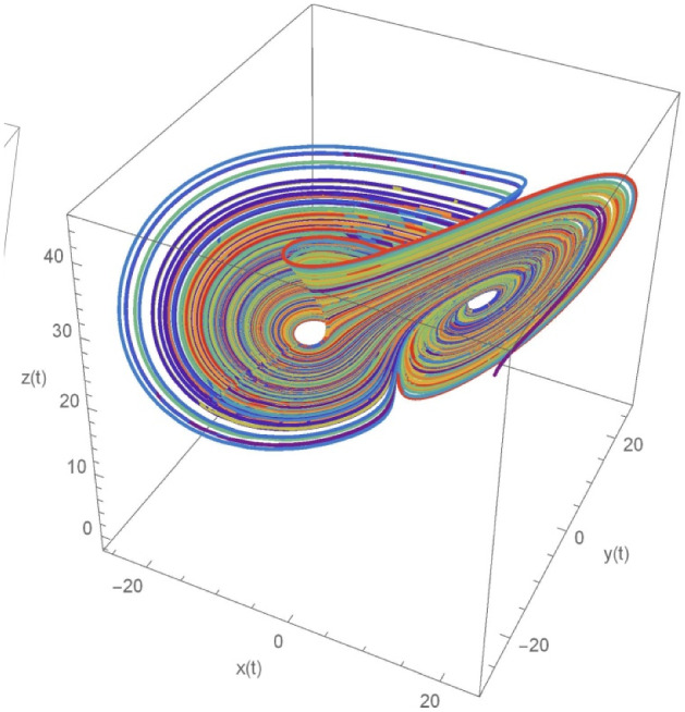
Example
Consider the following fractional Lorenz system of constant fractional order = 0.898 for the following system.
To find out the chaotic solution, we have considered and . The Fig. 1 illustrates the chaotic behaviour for and the result is compared with the work of Millici et al. [31] those are obtained using Runge–Kutta 4th order and Euler methods. Whereas Fig. 2 displays the exact solution of the system for .
Fig. 1.
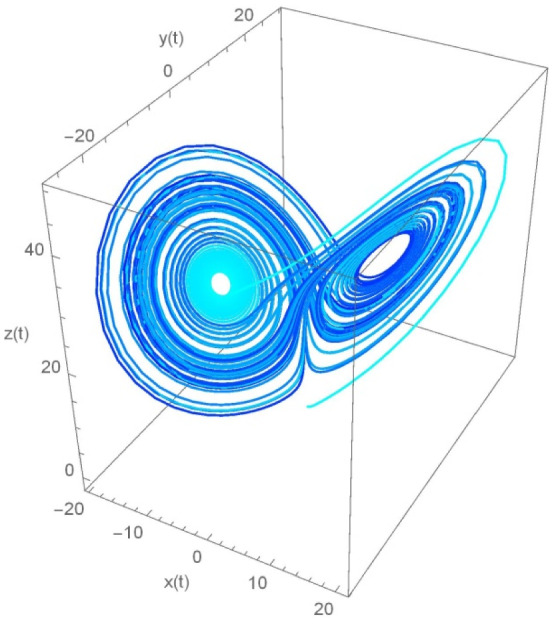
The fractional Lorenz system of order λ = 0.898
Fig. 2.
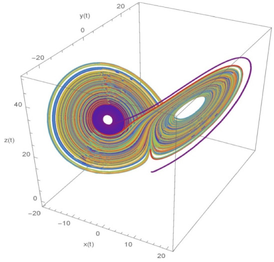
The exact solution of order λ = 1
Example 2
Let us consider the following fractional Lorenz system for the variable fractional order such that .
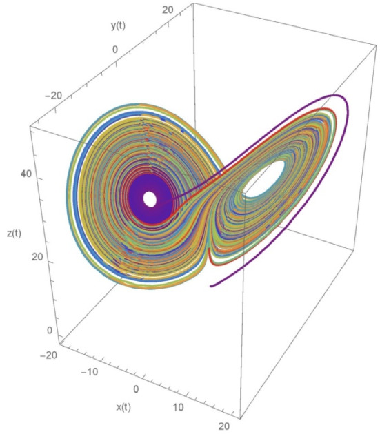
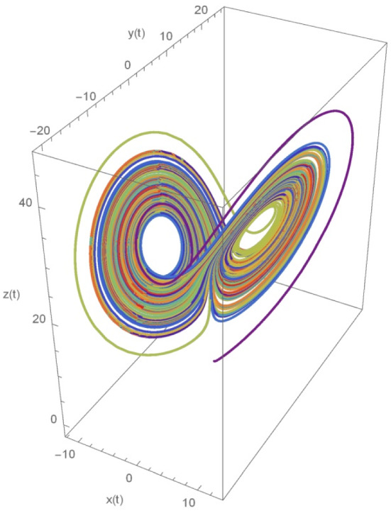
To find out the chaotic solution, we have considered and . The Fig. 3 illustrates the chaotic behaviour for and the result is compared with the work of Millici et al. [31] those are obtained using Runge–Kutta 4th order and Euler methods. Whereas Fig. 4 displays the exact solution of the similar system for .
Fig. 3.

The fractional Lorenz system of order λ(γ) = sin (γ)
Fig. 4.
The exact Lorenz system of order λ(γ) = 1
Example 3
Let us consider the following fractional Lorentz system of variable order such that and assuming for the following system.
To find out the chaotic solution, we have considered and . The Fig. 5 illustrates the chaotic behaviour for and the result is compared with the work of above Examples 1 and 2. Whereas Fig. 6 displays the exact solution of the similar system for
Fig. 5.

The fractional Lorenz system of order
Fig. 6.
The exact Lorenz system of order λ(γ) = 1
Example 4
Considering fractional Liu system of variable order such that .
To find out the chaotic solution, we have considered and . The Fig. 7 illustrates the chaotic behaviour for and the result is compared with the work of Millici et al. [31] those are obtained using Runge–Kutta 4th order and Euler methods. Whereas Fig. 8 displays the exact solution of the similar system for .
Fig. 7.

The fractional Liu system of order
Fig. 8.
The exact Liu system of order λ (γ) = 1
Conclusion
An analysis is carried out for the solution of variable fractal-fractional differential equations that overrides the fact of constant order. A new operator for both differential and integral is proposed for a continuous differentiable function involving power law assumption that utilizes to achieve Lipschitz condition. It is found that for a bounded function the derivative and integral associated to it also bounded. A new numerical scheme is employed for the solution of ODEs with the help of three-point Lagrange’s interpolation that utilizes the proposed integral operators. The solution procedure will provide a wide scope for several engineering as well as industrial problems due to the replacement of constant to variable fractal and fractional order. Several properties for the new operator are presented more precisely following their corresponding derivation. Further, various set of differential equations related to real- world applications are solved for both constant and variable fractional order and their chaotic behaviours are displayed graphically. Finally, the comparison with classical differential equations is also presented showing a good correlation.
Author’s Contributions
All the authors have equally contributed to complete the manuscript, i.e. PJ has formulated the problem and verified the problem statement and completed the introduction section and checked the similarity with grammar, SNM has computed and simulated the numerical results and finally, SRM has completed the draft with results and discussion section and checked the overall.
Funding
Not applicable.
Availability of Data and Material
No data is used.
Code Availability
Not applicable.
Declarations
Conflict of interest
There is no conflict of interest to publish our paper in your esteemed journal.
Ethics Approval
The entire work is the original work of the authors.
Consent to Participate
Not applicable.
Consent for Publication
All the authors have given their consent to publish the paper.
Footnotes
Publisher's Note
Springer Nature remains neutral with regard to jurisdictional claims in published maps and institutional affiliations.
Contributor Information
P. Jena, Email: pjena25.pj@gmail.com
S. N. Mohapatra, Email: satyananda999@gmail.com
S. R. Mishra, Email: satyaranjan_mshr@yahoo.co.in
References
- 1.Oldham K, Spanier J. The Fractional Calculus, Theory and Applications of Differentiation and Integration to Arbitrary Order. New York: Academic Press,; 1974. [Google Scholar]
- 2.Podlubny I. Fractional Differential Equations. San Diego: Academic Press; 1999. [Google Scholar]
- 3.Katz VJ. Ideas of calculus in Islam and India. Math Mag. 1995;68(3):163–174. doi: 10.1080/0025570X.1995.11996307. [DOI] [Google Scholar]
- 4.Kumar D, Singh J, Baleanu D. A hybrid computational approach for klein-gor-don equations on cantor sets. Nonlinear Dyn. 2017;87(1):511–517. doi: 10.1007/s11071-016-3057-x. [DOI] [Google Scholar]
- 5.Singh J, Gupta PK, Rai KN. Homotopy perturbation method to space-time fractional solidification in a finite slab. Appl. Math. Mode. 2011;135(4):1937–1945. doi: 10.1016/j.apm.2010.11.005. [DOI] [Google Scholar]
- 6.Turkyilmazoglu M. Convergent optimal variational iteration method and applications to heat and fluid flow problems. Int. J. Numer. Methods Heat Fluid Flow. 2016;26:790–804. doi: 10.1108/HFF-09-2015-0353. [DOI] [Google Scholar]
- 7.Irandoust-Pakchin S, Javidi M, Kheiri H. Analytical solutions for the fractional nonlinear cable equation using a modified homotopy perturbation and separation of variables methods. Comput. Math. Phys. 2016;56(1):116–131. doi: 10.1134/S0965542516010103. [DOI] [Google Scholar]
- 8.Xu Y, Sun K, He S, Zhaog L. Dynamics of a fractional-order simplified unified system based on the adomian decomposition method. Eur. Phys. J. Plus. 2016;131(6):1–12. doi: 10.1140/epjp/i2016-16186-3. [DOI] [Google Scholar]
- 9.Ray SS, Gupta AK. Numerical solution of fractional partial differential equation of parabolic type with Dirichlet boundary conditions using two-dimensional Legendre wavelets method. J. Comput. Nonlinear Dyn. 2016;11(1):011012. doi: 10.1115/1.4028984. [DOI] [Google Scholar]
- 10.Rayal A, Verma SR. Two-dimensional Gegenbauer wavelets for the numerical solution of tempered fractional model of the nonlinear Klein-Gordon equation. Appl. Numer. Math. 2022;174:191–220. doi: 10.1016/j.apnum.2022.01.015. [DOI] [Google Scholar]
- 11.Sene N. Study of a fractional-order chaotic system represented by the caputo operator. Complex. 2021;2021:5534872. doi: 10.1155/2021/5534872. [DOI] [Google Scholar]
- 12.Goswami P, Alqahtani RT. On the solution of local fractional differential equations using local fractional Laplace variational iteration method. Math. Probl. Eng. 2016;2016:9672314. doi: 10.1155/2016/9672314. [DOI] [Google Scholar]
- 13.Sun HG, Chen W, Wei H, Chen Y. A comparative study of constant-order and variable-order fractional models in characterizing memory property of systems. Eur. Phys. J. Spec. Top. 2011;193(1):185–192. doi: 10.1140/epjst/e2011-01390-6. [DOI] [Google Scholar]
- 14.Zhang H, Liu F, Phanikumar MS, Meerschaert MM. A novel numerical method for the time variable fractional order mobile-immobile advection-dispersion model. Comput. Math Appl. 2013;66(5):693–701. doi: 10.1016/j.camwa.2013.01.031. [DOI] [Google Scholar]
- 15.Samko SG, Ross B. Integration and differentiation to a variable fractional order. Integr. Transf. Spec. Funct. 1993;1(4):277–300. doi: 10.1080/10652469308819027. [DOI] [Google Scholar]
- 16.Coimbra CFM. Mechanics with variable-order differential operators. Ann. Der Phys. 2003;12(11–12):692–703. doi: 10.1002/andp.200351511-1203. [DOI] [Google Scholar]
- 17.Ali F, Sheikh NA, Khan I, Saqib M. Magnetic field effect on blood flow of Casson fluid in axisymmetric cylindrical tube: a fractional model. J. Magn. Magn. Mater. 2017;423:327. doi: 10.1016/j.jmmm.2016.09.125. [DOI] [Google Scholar]
- 18.Owolabi KM. Robust and adaptive techniques for numerical simulation of nonlinear partial differential equations of fractional order. Commun. Nonlinear Sci. Numer. Simul. 2017;44:304. doi: 10.1016/j.cnsns.2016.08.021. [DOI] [Google Scholar]
- 19.Chen W. Chaos, Soliton. Fractals. 2016;28:9239. [Google Scholar]
- 20.Atangana A, Qureshi S. Modelling attractors of chaotic dynamical systems with fractal-fractional operators. Chaos Solitons Fract. 2019;123:320–337. doi: 10.1016/j.chaos.2019.04.020. [DOI] [Google Scholar]
- 21.Caputo M, Fabrizio M. A new definition of fractional derivative without singular kernel. Prog. Fract. Differ. Appl. 2015;1(2):73–85. [Google Scholar]
- 22.Aguilar JFG. Irving-mullineux oscillator via fractional derivatives with Mittag–Leffler kernel. Chaos Solitons Fract. 2017;95:179–186. doi: 10.1016/j.chaos.2016.12.025. [DOI] [Google Scholar]
- 23.Salahshour S, Ahmadian A, Allahviranloo T. A new fractional dynamic cobweb model based on nonsingular kernel derivatives. Chaos Solitons Fractals. 2021;145:110755. doi: 10.1016/j.chaos.2021.110755. [DOI] [Google Scholar]
- 24.Shloof AM, Senu N, Ahmadian A, Pakdaman M, Salahshour S. A new iterative technique for solving fractal-fractional differential equations based on artificial neural network in the new generalized caputo sense. Eng. Comput. 2022 doi: 10.1007/s00366-022-01607-8. [DOI] [Google Scholar]
- 25.Shloof AM, Senu N, Ahmadian A, Nik Long NMA, Salahshour S. Solving fractional-fractal differential equations using operational matrix of derivatives via Hilfer fractal-fractional derivative sense. Appl. Numer. Math. 2022;178:386–403. doi: 10.1016/j.apnum.2022.02.006. [DOI] [Google Scholar]
- 26.Zhou J, Salahshour S, Ahmadian A, Senu N. Modeling the dynamics of COVID-19 using fractal-fractional operator with a case study. Res. Phys. 2022;33:105103. doi: 10.1016/j.rinp.2021.105103. [DOI] [PMC free article] [PubMed] [Google Scholar]
- 27.Haidong Q, Rahman M, Arfan M, Salimi M, Salahshour S, Ahmadian A. Fractal-fractional dynamical system of Typhoid disease including protection from infection. Eng. Comput. 2021 doi: 10.1007/s00366-021-01536-y. [DOI] [Google Scholar]
- 28.Shloof AM, Senu N, Ahmadian A, Salahshour S. An efficient operation matrix method for solving fractal-fractional differential equations with generalized caputo-type fractional-fractal derivative. Math. Comput. Simul. 2021;188:415–435. doi: 10.1016/j.matcom.2021.04.019. [DOI] [Google Scholar]
- 29.Zhang L, Rahman M, Haidong Q, Adnan AM. Fractal-fractional Anthroponotic Cutaneous Leishmania model study in sense of Caputo derivative. Alexandria Eng. J. 2022;61:4423–4433. doi: 10.1016/j.aej.2021.10.001. [DOI] [Google Scholar]
- 30.Rayal A, Verma SR. Numerical analysis of pantograph differential equation of the stretched type associated with fractal-fractional derivatives via fractional order Legendre wavelets. Chaos Solitons Fractals. 2020;139:110076. doi: 10.1016/j.chaos.2020.110076. [DOI] [Google Scholar]
- 31.Tate S, Dinde HT. Some theorems on Cauchy problem for nonlinear fractional differential equations with positive constant coefficient. Mediterr J. Math. 2017;14:16–41. doi: 10.1007/s00009-017-0886-x. [DOI] [Google Scholar]
- 32.Aghajani A, Pourhadi E, Trujillo J. Application of measure of noncompactness to a Cauchy problem for fractional differential equations in Banach spaces. Fract. Calculus Appl. Anal. 2013;16(4):962–977. doi: 10.2478/s13540-013-0059-y. [DOI] [Google Scholar]
- 33.Atangana A, Shafiq A. Differential and Integral operators with Constant fractional order and Variable fractional Dimension. Chaos Solitons Fractals. 2019;127:226–243. doi: 10.1016/j.chaos.2019.06.014. [DOI] [Google Scholar]
- 34.Atangana A, Jain S. A new numerical approximation of the fractal ordinary differential equation. Eur. Phys. J. Plus. 2018;133:37. doi: 10.1140/epjp/i2018-11895-1. [DOI] [Google Scholar]
Associated Data
This section collects any data citations, data availability statements, or supplementary materials included in this article.
Data Availability Statement
No data is used.
Code Availability
Not applicable.