

Abstract
Kolkata has a reputation for being one of the world’s most polluted cities, particularly in the post-monsoon months of October, November, and December. Diwali, a Hindu festival, coincides with these months where a large number of firecrackers are set off followed by high emissions of air pollutants. As a result, the air quality index (AQI) deteriorates to “very poor” (301 ≤ AQI ≤ 400) and “poor” (201 ≤ AQI ≤ 300) categories. This situation stays for several days to a month. The present study aims to identify the thresholds for PM2.5 and PM10 that cause the AQI of Kolkata to deteriorate to “very poor” and “poor.” For this purpose, we have used a rough set theory-based condition-decision support system to predict the aforementioned categories of AQI. We have developed a Z-number-based novel quantification measure of semantic information of AQI to assess the reliability of the outcomes, as generated from the condition-decision-based decision rules, during post-monsoon season. The result reveals the best possible forecast of AQI with linguistic summarization of the reliability or confidence for different threshold ranges of PM10 and PM2.5. Inverse-decision rules based on rough set theory are utilized to justify and validate the forecasts. The explainability of the condition-decision support system is demonstrated/visualized using a flow graph that maps rough-rule-based different decision paths between input and output with strength, certainty, and coverage. The investigation resulted in an advanced intelligent environmental decision support system (IEDSS) for air-quality prediction.
Keywords: AQI, Condition-decision support system, Explainable AI, Flow graph, Machine intelligence, PM2.5, PM10, Rough sets, Z-numbers
Introduction
Prediction of air quality is a major challenge in early warning and control of urban air pollution. With the steep increase of urbanization and the advancement of industrialization, the problem of urban air pollution has become significantly important, as it accelerates climate change and affects human health. The post-monsoon months of October, November, and December coincide with Diwali, India’s most important religious holiday. As a part of the celebration, a large amount of firing crackers get burnt starting from late evening to late night on the Diwali day, as well as before and after Diwali. Metallic chemicals such as salts of potassium, sodium, strontium, barium and copper, charcoal, iron, sulphur, manganese, and aluminum dust powder are found in fireworks. After these chemicals get burnt, gaseous pollutants are generated which are harmful for the environment and, in turn, put our health at stake.
Air pollution is one of the most serious global health and environmental concerns which is more prevalent in urban areas. It is caused by anthropological activities that degrade ecological balance and kill millions of people each year. In many cities where unplanned urbanization occurs, air pollution exceeds danger limits in terms of human health, posing a health threat or affecting life quality (Cetin & Sevik, 2016a; Singh et al., 2020). Cetin (2016) showed how the indoor CO2 parameters influence the students’ performance of activity in the examination halls. Cetin and Sevik (2016b) studied the effects of indoor plants on the concentration of CO2 in an indoor environment under certain light conditions. Cetin et al. (2019) evaluated the air quality based on CO2 amount and amount of particulate matter in 6 different dimensions and determined the change in sound level on a regional basis depending on the time of day and the season in different areas of Bursa City Center. In Elsunousi et al. (2021), the regional and periodic change of CO2 and particulate matter pollution in the city of Misurata were illustrated. Climate has a direct impact on a plant’s characteristics (Kaya et al., 2019; Sevik et al., 2021). Heavy metals are especially critical among the components of air pollution because they can be poisonous and deadly even at low concentrations, and even the necessary elements for organisms can be harmful at high concentrations (Jo et al., 2020). Since they are not easily decomposed, they tend to bioaccumulate, and some of them have toxic or carcinogenic effects even at low concentrations (Cetin & Jawed, 2022; Waaijers et al., 2012). Sevik et al. (2020a, b) determined the variation of Pb and Mg accumulation depending on plant species, plant organ, washing status, and traffic density in some landscape plants grown in the city center of Kastamonu. Cetin et al. (2020) used blue spruce (Picea pungens) tree organs to calculate the concentration of heavy metals, such as Ca, Cu, and Li in the city of Ankara. Fruits and vegetables cultivated in industrial and urban areas with significant levels of heavy metal pollution can be detrimental to public health if consumed as crops (Sevik et al., 2020a, b). The most preferred method for determining the changes in heavy metal concentrations in the atmosphere is the use of biomonitors, especially with the help of the annual growth rings of trees (Cesur et al., 2021). In this study, the changes in heavy metal concentrations in the annual rings of Cupressus arizonica tree growing in the city center of Kastamonu were observed. The effects of enhanced UV-B radiation on plant growth, development, biomass accumulation, yield, metabolism, and morphological characteristics of both germination and seedlings are significant (Kumar & Bhardwaj, 2019; Ozel et al., 2021). Excessive phosphorus and nitrogen pose a significant threat to the quality of freshwater lakes in Malaysia (Huang et al., 2015; Varol et al., 2022). In the worst scenarios, urban runoff contains enough pollutants to make it impossible for us to swim in or fish in our local waters. Porous plastic asphalt pavements provide an alternative technology for stormwater management (Cetin, 2013).
There have been many studies that show the impact of firework activities on air quality during the Diwali celebration in India. It has been found that fireworks cause short-term variation and degradation in air quality, as well as major changes in pollutant concentrations. In Hisar, for example, PM10 and TSPM concentrations are seen to increase by two to three times (Ravindra et al., 2003). Barman et al. (2008, 2009) found a considerable rise in PM2.5 levels in Lucknow. In case of Kolkata, the mass concentrations of PM10 and SO2 were found to be ~ 5 times the standard limits, as prescribed (Chatterjee et al., 2013). Mandal et al. (2022) recently examined the effect of pollution during Diwali celebrations of COVID-19 outbreak. Though most of the research has studied the change of air quality and its effect on the environment during Diwali compared to normal periods, modelling the air quality in terms of “cause-effect” relation for the purpose of predicting the probable ranges of pollutants during Diwali months remains an issue for researchers. Such modelling is helpful for environmentalists to mitigate the deterioration on air quality, and its consequences.
Intelligent decision support systems (IDSS) are developed by integrating the idea of decision support system (DSS) and artificial intelligence (AI) techniques judiciously. It often applies expert system technology to assist in the resolution of complex decision problems by adopting the knowledge of human experts with logical reasoning. An IDSS is expected, ideally, to act like a user-friendly human expert or consultant in providing support to decision-makers, e.g., by gathering and analyzing evidence, diagnosing problems, suggesting possible courses of actions, and evaluating those actions. Here, the use of AI techniques attempts to make these tasks performed efficiently by a machine with enhanced tractability to handle difficulties, while achieving close resemblance with human-like decision-making. Environmental problems are among the set of crucial domains in which inappropriate management decisions can have severe social, economic, and environmental implications. Decision provided by intelligent environmental decision support systems (IEDSSs) is significant in the interaction of humans and ecosystems as they are the instruments developed to deal with the multidisciplinary nature and high complexity of environmental challenges. In this scenario, statistical and artificial intelligence-based various data analysis tools and techniques can be judiciously integrated and used to give valuable environmental knowledge for the IEDSS decision-making process. AI techniques have been applied to environmental management problems for a long period with good results. AI tools like case-based reasoning, artificial neural networks, genetic algorithms, swarm intelligence, and decision trees were employed to develop various knowledge-based systems, expert systems, and fuzzy inference systems for this purpose (Ahmed et al., 2003; Riga et al., 2009; Dutta & Chaudhuri, 2014; Ong et al., 2015; Corominas et al., 2018; Qi et al., 2018; Abdul-Wahab et al., 2019; Zhao et al., 2019; Liu et al., 2019; Kuri-Monge et al., 2021).
Rough set theory, introduced by Pawlak (1991), provides important AI techniques for modelling complex data structures. It can effectively analyze various kinds of imprecise, inconsistent, incomplete, or imperfect information in order to find the hidden knowledge that can be used to discover a potential rule (Qu et al., 2020). Lin et al. (2011) used rule-based decision-making technique of rough set theory to predict customer churn in credit card accounts; they used a flow network graph and a path-dependent approach to infer decision rules and variables. Liou et al. (2016) used the rough set theory (RST) with flow graph in developing strategies to improve service quality. Stević et al. (2017) developed a multicriteria decision model with eight criteria and eight alternatives. Kundu and Pal (2018) introduced a new variant of rough set, namely, double bounded rough set, to quantify the tension force and proposed an algorithm based on tension measure is for link prediction. Chakraborty and Pal (2021) proposed rough set-based moving object background classification and motion uncertainty analysis with newly defined motion entropy. Rough set theory along with decision rules was employed for estimation of raw silk quality (Kar et al., 2021). The importance of the theory stems from the fact that it can show the probabilistic structure of the data being evaluated without having any prior knowledge. As a consequence, it is ideal for analyzing the probabilistic structures of data related to dynamic and non-linear meteorological phenomena. In meteorological research, the theory of rough sets is widely used. For example, Shan (2001) used a rough set-based approach to classify weather data. This theory was introduced for the prediction of drought by Liu and Qiao (2009). In addition, it was applied to assess the pollution sources of the atmospheric particulates of Jilin City both during the heating and non-heating periods (Fang et al., 2010). Chaudhuri and Dutta (2013) investigated the significance of GPT (generalized potential temperature) to define the humid condition of moist atmosphere for the predominance of the natural hazards by generating rough set theoretic “if–then” rules. Sudha (2017) proposed intelligent decision support system using rough sets and fuzzy logic for short-range rainfall prediction. A rough set-based decision support system has been used by Matarazzo (2018) for managing the air pollution in the industrial area. Rough set is found to be extremely suitable for classifying the air pollutant index in Malaysia and Singapore (Wibowo et al., 2018). Furthermore, the theory has been used to various uncertainty handling, and multicriteria decision-making applications (Kazemitash et al., 2021; Naouali et al., 2020; Pal et al., 2018; Saha et al., 2010; Suresh et al., 2012; Tang et al., 2020; Wang & Zhang, 2014; Ye et al., 2021). In our present study, we have used rough set-based “if–then” rules and inverse-decision rules for air-quality prediction and interpreting/explaining the decision-making process, respectively.
Decision-making in real-world problems is generally performed based on information that is often uncertain, ambiguous, incomplete, and/or imprecise. Fuzzy set theory of Zadeh (1965) is reputed in dealing with this kind of information. The effectiveness of the theory has been demonstrated in different domains, e.g., engineering, meteorology, economics, biological, social sciences, and computer science. In 2011, he defined Z-numbers (Zadeh, 2011), another new concept/measure concerning computing with words (CWW). This number provides a more general framework or structure for modelling/representing the uncertain information arising in real-world phenomena by incorporating the reliability of information. Since then, Z-number has been widely used in different fields like psychological research (Aliev & Memmedova, 2015), medical diagnosis (Wu et al., 2017), marketing (Alizadeh & Serdaroglu, 2016), multicriteria game model (Peng et al., 2019b), investment risk analysis (Peng et al., 2019a), natural language understanding (Banerjee & Pal, 2015), video tracking (Pal et al., 2019), and safety analytics (Das et al., 2020). Hendiani and Bagherpour (2019) used the concept of Z-numbers to model a possibilistic approach with the purpose of calculating the sustainability index in the context of reliability. A nice review on Z-numbers with different applications since its inception in 2011 has been recently reported (Banerjee et al., 2021). Z-numbers have not been used in the prediction of air quality so far. The present study is an attempt to demonstrate the significance of Z-numbers for quantifying the air quality in terms of linguistic abstraction. This concept is unique.
National air quality standards may vary depending on the approach adopted for balancing health risks, technological feasibility, economic considerations, and various other political and social factors, which, in turn, is influenced by other things such as the level of development and national capability in air quality management (Beig et al., 2010). Air quality index (AQI) is aimed at making decisions about how to protect the health of people by optimizing the short-term exposure to air pollution and controlling the activity levels when pollution levels are high. It assesses the current air quality, which is dependent on the specific level of concentration of an individual air pollutant. One may note that the air quality deteriorates during the Diwali festival in October–November, and the AQI remains high for several days to a month. For the post-monsoon months of October, November, and December, we consider AQI categories of “poor” (AQI within 201–300) and “very poor” (AQI within 301–400).
The present article describes the development of an intelligent environmental decision support system. It demonstrates the effectiveness of rough set theory-based decision rules, inverse-decision rules, flow graphs, and z-numbers in doing so. Interpretability is the ability to identify the relationships and counterfactuals between input and output, and the ability to search for evidence in the data that supports a particular outcome (Kovács et al., 2021). The use of the proposed inverse-decision rules provides interpretation/explanation of the decisions made on air-quality prediction. Flow graph that maps the rough-rule-based different paths between input and output with strength, certainty, and coverage enables visualization of the explainability of the condition-decision support system. Inverse rules in conjunction with Z-numbers thus enable interpretability of the proposed decision support system.
The novelty of the paper mainly lies in the following:
Modelling the AQI in terms of particulate matter (PM2.5 and PM10) using rough set theoretic “cause-effect”/ “if–then” relation for prediction of air quality during Diwali months
Developing a Z-number-based AQI that quantifies the abstraction of decision-making information concerning AQI prediction, which is first of its kind
Using rough set-based inverse-decision rules for determining the possible ranges of particulate matter (PM2.5 and PM10) that are responsible for a given air quality; this demonstrates the explainability of the system towards a decision
Designing an information flow graph between input and output that clearly demonstrates/visualizes the explainability of the condition-decision support system
All these novel features precisely illustrate how to integrate the merits of AI tools such as rough set-based condition-decision support system, inverse-decision rules with flow graph having explainability, and Z-numbers for quantification of semantic information to define AQI so as to design an advanced IEDSS for prediction and quantification of air quality during Diwali.
Material and methods
Study area
Kolkata (erstwhile Calcutta) is one of the large metropolitan cities of India. It is in the Ganges Delta at 22°33′North and 88°20′East, along the eastern side of the Hooghly River at an elevation of about 9 m. Kolkata is a densely populated city with a population of 14.4 million. It is included in the world’s twenty-five severely polluted cities including ten others from India (Bera et al., 2020) facing rising air pollution and multi-pollutant crisis. The city’s economic and industrial expansion, as well as different industries (paper and pulp, rubber, iron, plastic, textile, and food), vehicular emissions, dust from construction sites, solid waste burning, wind-blown dust from open lands, and thermal power plants, all contribute significantly to air pollution in Kolkata. As a result, the air quality in this area has deteriorated considerably. According to a study conducted at major traffic intersections in Kolkata, the levels of significant pollutants, such as PM10, NO2, CO, SO2, and lead, are found to be substantially higher than the permitted values (Ghose et al., 2004). Kolkata, like the rest of India, celebrates Diwali together along with “Kali Puja” festival with eagerness and devotion. A large number of crackers and sparklers of different kinds and intensities get burnt on the day of Diwali and also the adjacent days before and after.
Data collection and data pre-processing
The location of Kolkata and the data from twenty monitoring stations are shown in Fig. 1. These twenty monitoring stations are Dunlop Bridge, Rabindrabharati, Shyambazar, Victoria Memorial, Ultadanga, Beliaghata, Moulali, Salt Lake, Minto Park, Topsia, BITM, Hyde Road, Gariahat, Jadavpur, Fort William, Rabindra Sarobar, Tollygunge, Mominpore, Behala Chowrasta, and Baishnabghata. We have conducted our study based on the data and observations of 7 years from 2015 to 2021 over Kolkata, India, during October, November, and December. The data of daily air quality of Kolkata city is obtained from the West Bengal Pollution Control Board (WBPCB). Our present study considers two pollutants, namely, PM2.5 and PM10 (particulate matter of size 10 μm or less and 2.5 μm or less, respectively).
Fig. 1.

Location of the Kolkata metropolitan area and air monitoring stations
After collecting the data, pre-processing is executed to improve the data quality. Missing data is a common problem for most air pollution monitoring stations due to instrument failure, data entry error, maintenance, and other unmanageable factors. Though there are a few missing values in our data record, to fill the empty values, a linear interpolation technique is used.
Methodology: tools and definitions
Here, we provide some basic definitions and AI tools which are employed in formulating the proposed methodology for air-quality prediction. These include information table, decision table, and characteristics of decision rules in the framework of rough set theory. These are followed by the concept of flow graph and Z-numbers.
Information system and decision table
An information system (Pawlak, 2004) can be viewed as a data table (matrix) where columns denote different attributes, the rows denote different objects of interest, and the entries of the table represent attribute values. This is represented as a pair of sets as (Pawlak, 2004)
| 1 |
Here, U and A represent the universe of objects and the set of attributes, respectively. These are non-empty finite sets. , where is the set denoting all values of a, referred to as the domain of a, for each . Any subset B of A characterizes/determines a binary relation on U. This is also known as an indiscernibility relation, described as (Pawlak, 2004)
| 2 |
Here, denotes the value of the attribute a corresponding to element . is an equivalence relation. or simply by denotes the family of equivalence classes caused by , i.e., partitions on as determined by . represents the block of the partition that contains x.
If , then and are said to be B-indiscernible (indistinguishable) with respect to attribute-subset B.
If we arrange an information system in two distinct classes of attributes, namely, condition and decision attributes, then it is called a decision system, defined by (Pawlak, 2004)
| 3 |
where and are two disjoint sets of condition and decision attributes. . and denote the condition class and decision class as introduced by , respectively.
A decision system may also be referred as a decision table that represents various decisions (e.g., actions and results) made when some conditions get satisfied. That means, each row of the table represents a decision rule that characterizes decisions in terms of conditions.
Decision rules: characteristic features (Pawlak, 2004)
Let represent a decision table as mentioned above. Let every determine a sequence given by
where and .
The sequence (Eq. 4) may be called a decision rule induced by (in ) and represented as
| 4 |
In brief, .
This decision rule is characterized by the following features:
-
Support of the decision rule
Support is a number defined as5 - Strength of the decision rule
where denotes the cardinality of a set .6 -
Certainty factor of
7 8 If = 1, then indicates a certain decision rule; otherwise not.
- Coverage factor of
9 10 Inverse-decision rule of
If represents a decision rule, then represents its inverse-decision rule.
Inverse-decision rules have been utilized in our proposed prediction methodology to provide explanations (reasons) or justification behind any decision taken.
Information flow graph
Information flow graph (Pawlak, 2005) maps the decision paths from input to output of a rough rule base. Accordingly, it provides a special kind of database in which statistical features of different objects are described in terms of information flow distribution rather than the raw data about individual objects. This type of data representation provides new insights into data structures and enables data analysis in more intelligent way.
A flow graph is a directed acyclic finite graph defined as (Pawlak, 2005)
| 11 |
Here, N denotes a set of nodes, represents a set of directed branches, and denotes a flow function where is the set of non-negative reals. Each node of the flow graph represents an attribute of the information system.
The basic concepts (Pawlak, 2005) of the flow graph G are as follows:
If , then x is an input of y, and y is an output of x.
If , then I(x) and O(x) denote the sets of all x’s inputs and outputs.
- Input and output of G are defined as
12
Every node x in G is associated with its inflow and outflow as (Ramanna & Chitcharoen, 2013)
| 13 |
| 14 |
Similarly, the inflow and outflow for the whole flow graph G are represented as
| 15 |
| 16 |
The inflow and outflow of an internal node of a graph are supposed to be the same, and hence of the graph G (Pal & Chakraborty, 2017).
A normalized flow graph can be characterized by .
Here, N and are as in Eq. (11).
denotes the strength of a branch in , where
| 17 |
of a branch indicates the percentage of the total flow through it. Its higher value means larger percentage of flow.
Certainty (cer) and coverage (cov) factors of a branch (x, y) in are expressed as
| 18 |
| 19 |
Z-numbers
Z-number (Zadeh, 2011) is based on fuzzy set theory. This has been useful in computing with words (CWW) (Zadeh, 1996). In CWW, the perceptions are encoded in the words and phrases that are used to describe various events. This phenomenon is inspired by the exceptional ability of the human brain in making perception-based decisions. The underlying concept of Z-number characterizes the certainty of information (Pal et al., 2019).
A Z-number has two tuples, and is defined as
| 20 |
Tuple A, which is a constraint, is allowed to take the values of X (a real-valued uncertain variable, interpreted as the subject of Y). Tuple B is a measure of reliability of A. They are usually fuzzy numbers representing words or clauses in a natural language (Banerjee & Pal, 2013).
Let us consider a statement Y = Tropical cyclones are likely to become severe.
Here,
X = intensity of tropical cyclones, A = severe, B = likely, and the Z-based information of the statement is,
| 21 |
Thus, the uncertainty and fuzziness that occur in linguistic terms best suit the restriction and the reliability metric of Z-numbers. Z-number in terms of linguistic terms provides a natural way of interpretation and enhances the flexibility and reliability of decision-making systems. A detailed review on Z-numbers with its various applications made so far since its inception in 2011 is available in Banerjee et al. (2022). In our present study, we have employed Z-numbers as the linguistic measure of the reliability of the condition-decision support system to characterize the different criteria of the AQI.
Formulation of methodology
Different ranges of pollutants
The air quality index or AQI is a daily air quality measure which can be used to quantify concentration of pollutants. It is a measurement of how air pollution affects a person’s health with a small duration. The air quality index is composed of eight pollutants, i.e., particulate matters PM2.5 (size 2.5 μm or less) and PM10 (size 10 μm or less), sulphur dioxide (SO2), ammonia (NH3), nitrogen dioxide (NO2), carbon monoxide (CO), lead (Pb), and ozone (O3). The Central Pollution Control Board (CPCB) used the following methodology to calculate the AQI:
The general equation for the sub-index () for pollutant P for a given pollutant concentration () is
| 22 |
Here,
= sub-index for pollutant P
= rounded concentration of pollutant P
= breakpoint that is greater than or equal to
= breakpoint that is less than or equal to
= AQI value corresponding to
= AQI value corresponding to
The highest sub-index, , represents the AQI of the location.
The sub-indices for individual pollutants are calculated using its 24-hourly average concentration value (8-hourly in case of CO and O3) at a monitoring location. It is not always possible that all the eight pollutants to be monitored in all the locations. The overall AQI is determined only if the data for at least three pollutants are available, one of which must be either PM2.5 or PM10. Otherwise, the data is considered insufficient for computing the AQI. For sub-index calculation, a minimum of 16 h of data is required. Even if the data are insufficient to determine the AQI, the sub-indices for monitored pollutants are computed and disseminated. In that case, the individual pollutant-wise sub-index will provide the air quality status for that pollutant. The AQI is provided in real-time basis through the web-based system. It is an automated system that collects data from continuous monitoring stations without the need for human interaction and displays the AQI based on running average values (for example, AQI at 6 a.m. on a day will incorporate data from 6 a.m. on previous day to the current day). For manual monitoring stations, an AQI calculator has been developed where data can be manually entered to obtain AQI value.
The AQI classifications used below are provided by the CPCB of India. Here, AQI is measured on a six-point scale: severe, very poor, poor, moderate, satisfactory, and good. Table 1 illustrates different categories of AQI and the corresponding health impacts. The AQI values and corresponding ambient concentrations (health breakpoints) for the identified eight pollutants are presented in Table 5.
Table 1.
Different categories of national air quality index (AQI) with health impact (CPCB, 2014)
| AQI | Remark | Possible health impacts |
|---|---|---|
| 0–50 | Good | Minimal impact |
| 51–100 | Satisfactory | Minor breathing discomfort to sensitive people |
| 101–200 | Moderate | Breathing discomfort to the people with lung, heart disease, children and older adults |
| 201–300 | Poor | Breathing discomfort to people on prolonged exposure |
| 301–400 | Very poor | Respiratory illness to the people on prolonged exposure |
| > 400 | Severe | Respiratory effects even on healthy people |
Table 5.
Breakpoints for AQI scale 0–500 (units: μg/m3 unless mentioned otherwise) (CPCB, 2014)
| AQI category (range) |
PM10 24-h |
PM2.5 24-h |
NO2 24-h |
O3 8-h |
CO 8-h (mg/m3) |
SO2 24-h |
NH3 24-h |
Pb 24-h |
|---|---|---|---|---|---|---|---|---|
| Good (0–50) | 0–50 | 0–30 | 0–40 | 0–50 | 0–1.0 | 0–40 | 0–200 | 0–0.5 |
| Satisfactory (51–100) | 51–100 | 31–60 | 41–80 | 51–100 | 1.1–2.0 | 41–80 | 201–400 | 0.6–1.0 |
| Moderate (101–200) | 101–250 | 61–90 | 81–180 | 101–168 | 2.1–10 | 81–380 | 401–800 | 1.1–2.0 |
| Poor (201–300) | 251–350 | 91–120 | 181–280 | 169–208 | 10.1–17 | 381–800 | 801–1200 | 2.1–3.0 |
| Very poor (301–400) | 351–430 | 121–250 | 281–400 | 209–748* | 17.1–34 | 801–1600 | 1201–1800 | 3.1–3.5 |
| Severe (401–500) | 430 + | 250 + | 400 + | 748 +* | 34 + | 1600 + | 1800 + | 3.5 + |
*One hourly monitoring (for mathematical calculation only)
Due to Diwali festival during October–November, AQI deteriorates to “very poor” and “poor” categories and remains high for about a month. In our present study, we have dealt with the cases of two AQI categories, viz., “very poor” (AQI within 301–400) and “poor” (AQI within 201–300) during the post-monsoon month of October, November, and December. For the purpose of the identification of the influence of the burning of firecrackers on AQI, we have considered two pollutants, viz., PM2.5 and PM10, as these are most important to affect the air quality.
The air quality data of the year 2015–2019 are used as design set and that of 2020–2021 are used for validation (validation set). The concentration of PM2.5 during the post-monsoon months is found to be in the range of (91–270) µg/m3 having AQI categories “poor” and “very poor” with our 7 years of study period. The concentration values of PM2.5 are divided into four parts using normal probability distribution as follows: 91 ≤ PM2.5 ≤ 135, 136 ≤ PM2.5 ≤ 180, 181 ≤ PM2.5 ≤ 225, and 226 ≤ PM2.5 ≤ 270. Similarly, the concentration of PM10, having the range of (143–334) µg/m3 with AQI categories “poor” and “very poor” is categorized using normal probability distribution as follows: 143 ≤ PM10 ≤ 190, 191 ≤ PM10 ≤ 238, 239- ≤ PM10 ≤ 286, and 287 ≤ PM10 ≤ 334.
Framing of decision rules
The decision rules are constructed in terms of “condition–decision,” “cause–effect,” or “if–then” relations using rough set theory. The effectiveness of these rules is demonstrated by confirming the ranges of PM10 and PM2.5 for the predominance of the “poor” and “very poor” AQI. The decision rules with different conditions are framed as follows:
Fact 1: If (91 ≤ PM2.5 ≤ 135), then (AQI is poor or very poor)
Fact 2: If (136 ≤ PM2.5 ≤ 180), then (AQI is poor or very poor)
Fact 3: If (181 ≤ PM2.5 ≤ 225), then (AQI is poor or very poor)
Fact 4: If (226 ≤ PM2.5 ≤ 270), then (AQI is poor or very poor)
Fact 5: If (143 ≤ PM10 ≤ 190), then (AQI is poor or very poor)
Fact 6: If (191 ≤ PM10 ≤ 238), then (AQI is poor or very poor)
Fact 7: If (239- ≤ PM10 ≤ 286), then (AQI is poor or very poor)
Fact 8: If (287 ≤ PM10 ≤ 334), then (AQI is poor or very poor)
Flow graphs are generated corresponding these two sets of rules. These graphs depict different paths between input and output representing different decision rules with their respective strength, certainty, and coverage values.
Z-number-based AQI
In our investigation, the concept of Z-numbers is employed to develop metrics (indices) characterizing the air quality in the month of October, November, and December during Diwali time. As stated before, our objective is to identify different threshold ranges of PM2.5 and PM10 responsible for AQI value to be “poor” and “very poor.” Rough set theoretic condition–decision support system is used to quantify the information associated with decision rules. Every decision rule has certainty and coverage factors. The certainty value describes the conditional probability that an object belongs to the decision class indicated by the decision rule as well as it meets the condition of the rule. In contrary, coverage value illustrates the conditional probability of justifications behind a particular decision (Chaudhuri & Dutta, 2013). Based on the results obtained using rough set theory, the Z-based information of B is provided (Eq. 20). A of the Z-number is defined as a group of classes having similar criteria that define AQI. Here, we only consider two criteria of AQI, namely, poor and very poor. That is, A = {poor, very poor} where “poor” denotes AQI value within the range of 201–330 and “very poor” denotes AQI value within the range of 301–400. B is a measure of the degree of sureness regarding the value of A. As mentioned, while defining the Z-numbers above, A and B are usually fuzzy numbers denoting words or phrases. Determination of B is done with the help of the certainty and coverage values obtained from Eqs. (7) and (9). B is the set of reliability values, e.g., B = {Certainly, Most Likely, Likely, Less Likely, May be, Unlikely}.
The criteria for Z-number are defined as in Table 2. For example, if certainty is within the range of 0.70 ≤ Certainty ≤ 1 and coverage also lies within the range of 0.70 ≤ Coverage ≤ 1 or vice versa, then it is labeled as “Certainly.” If the said AQI is “poor,” then the Z-based information can be written as Z = < poor, Certainly > . Thus, this Z-based metric can also be used as an index to determine whether an AQI is “poor” or “very poor.” The label “May be” denotes an unusual range where the certainty lies within the range of 0.60 ≤ Certainty ≤ 1 and the coverage lies within the range of 0.01 ≤ Coverage < 50, or vice versa.
Table 2.
Ranges of certainty and coverage and corresponding linguistic description using Z-number
| Ranges of certainty and coverage | Z-number-based information |
|---|---|
| 0.70 ≤ Certainty ≤ 1 and 0.70 ≤ Coverage ≤ 1 | Certainly |
|
0.60 ≤ Certainty ≤ 1 and 0.50 ≤ Coverage ≤ 1 or 0.60 ≤ Coverage ≤ 1 and 0.50 ≤ Certainty ≤ 1 |
Most Likely |
| 0.50 ≤ Certainty < 70 and 0.50 ≤ Coverage < 70 | Likely |
| 0.20 ≤ Certainty < 0.50 and 0.20 ≤ Coverage < 0.50 | Less Likely |
|
0.60 ≤ Certainty ≤ 1 and 0.01 ≤ Coverage < 50 or 0.60 ≤ Coverage ≤ 1 and 0.01 ≤ Certainty < 50 |
May be |
| 0.00 ≤ Certainty < 0.20 and 0.00 ≤ Coverage < 0.20 | Unlikely |
Validation and inverse-decision rules
We validate the decision rules using the post-monsoon air quality data of the years 2020 and 2021. As mentioned earlier, inverse-decision rules are framed during validation time with the validation set. These inverse-decision rules are used to provide justifications (reasons) for given decisions. These are as follows:
Inverse Fact 1: If AQI is (poor or very poor), then (91 ≤ PM2.5 ≤ 135)
Inverse Fact 2: If AQI is (poor or very poor), then (136 ≤ PM2.5 ≤ 180)
Inverse Fact 3: If AQI is (poor or very poor), then (181 ≤ PM2.5 ≤ 225)
Inverse Fact 4: If AQI is (poor or very poor), then (226 ≤ PM2.5 ≤ 270)
Inverse Fact 5: If AQI is (poor or very poor), then (143 ≤ PM10 ≤ 190)
Inverse Fact 6: If AQI is (poor or very poor), then (191 ≤ PM10 ≤ 238)
Inverse Fact 7: If AQI is (poor or very poor), then (239- ≤ PM10 ≤ 286)
Inverse Fact 8: If AQI is (poor or very poor), then (287 ≤ PM10 ≤ 334)
The same criteria for Z-number as mentioned in Table 2 are used while implementing inverse rules. The overall research framework is illustrated in a block diagram (Fig. 2).
Fig. 2.
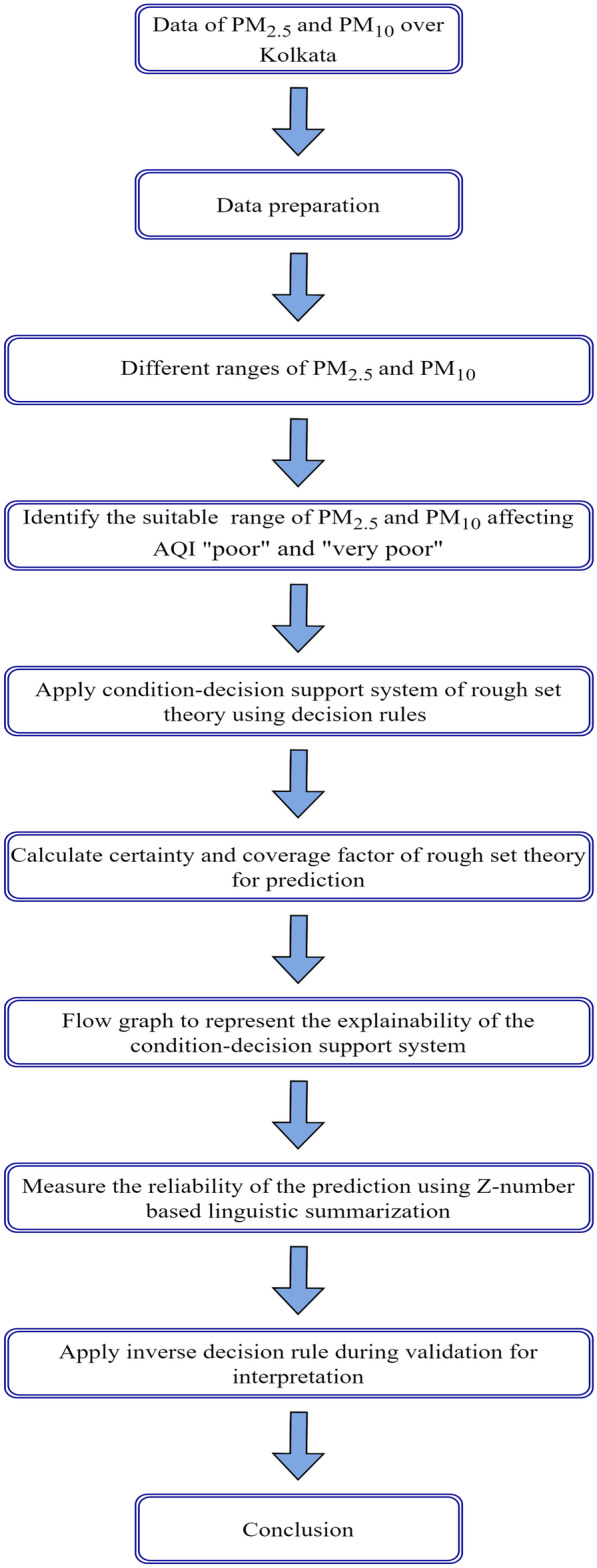
Block diagram showing proposed research framework
Results and discussion
Variation in PM2.5 and PM10 during Diwali
On a normal, pre-Diwali, Diwali, or post-Diwali day, the diurnal variation (6–6 a.m.) of PM10 and PM2.5 is illustrated in Fig. 3 based on the Diwali data during 2019, as an example. It is observed that the daytime PM10 and PM2.5 concentrations on normal and pre-Diwali days are clearly similar and lower than those on Diwali and post-Diwali days. However, the concentrations of PM10 and PM2.5 were consistently greater at night than during the day time. During the Diwali, as well as before (pre) and after (post) Diwali, the night-time concentrations of PM10 and PM2.5 peaked between 8 p.m. and 3 a.m., indicating that the majority of the firework activity took place during that time. The influence of firework activity during the night lasted until the next day morning, as we found that the concentrations of these two pollutants increase on the Diwali and post-Diwali days during 6 a.m.–1 p.m. as compared to pre-Diwali and normal days. The pollution levels remained high from several days to about a month instead of subsiding after the Diwali. PM, generated during firecracker burning, has an important part in the environment since various ions and particles adsorbed by them. Both PM10 and PM2.5 can penetrate the respiratory system; however, atmospheric particulate matter PM2.5 which is about 3% the diameter of a human hair is more harmful because it can travel deep into the lungs and cause a wide range of respiratory and cardiovascular diseases, as well as cancer.
Fig. 3.

Diurnal variation of a PM2.5 and b PM10 during Diwali, pre-Diwali, post-Diwali, and normal day
Flow graph and explainability
As stated earlier, a flow graph is associated with a decision table. It is a directed acyclic graph in which a directed branch x connects the input and output nodes (viz., C(x) and D(x), respectively) corresponding to a decision rule . The through flow of a branch is represented by the decision rule’s strength factor (Pawlak, 2004). Figures 4 and 5 show graphical representation of two flow graphs corresponding to PM2.5 and PM10. As mentioned earlier, the concentrations of PM2.5 and PM10 are divided into four ranges, so there are four roots for each of PM2.5 and PM10 satisfying the decisions — “poor” and “very poor” AQI. Every root covers some strength, certainty, and coverage values which are visualized easily with the help of flow graph. This representation enables determining the probable roots for each prediction with priority.
Fig. 4.

Flow graph for the decision algorithm of PM2.5
Fig. 5.

Flow graph for the decision algorithm of PM10
The term “explainable AI” or “interpretable AI” refers to human being able to understand the path that artificial intelligence technology took to make a decision using dynamically generated graphs or textual descriptions. Flow graphs in Figs. 4 and 5 that represent two decision tables provide a clear insight into the decision-making process with strength, certainty, and coverage values; thereby demonstrating the interpretation ability or explanation ability of the proposed condition-decision support system to make air-quality prediction.
Results of condition-decision support system using design set
In this study, we apply rough set theory to identify the threshold ranges of PM2.5 and PM10 that make degradation of air quality in the months of October, November, and December during Diwali over Kolkata. We consider the certainty and coverage values of a rough set theoretic rule for a specific decision with different conditions. These values were obtained using Eqs. (7) and (9), respectively. Higher values of certainty and coverage mean better prediction. Every decision rule has two parts — condition (i.e., different ranges of pollutants) and decision (i.e., AQI categories). Figure 6 displays “poor” and “very poor” AQI which are caused by different threshold ranges of PM2.5. With the range (91–135) µg/m3, i.e., 91 ≤ PM2.5 ≤ 135 (Fact 1), the higher values of certainty (0.70) and coverage (1.00) are obtained when AQI is “poor” (Fig. 6a). Here, the certainty factor of 0.70 for the said rule means, 70% of the days fulfil the condition and the decision of the same rule, and 30% are missed predictions. Furthermore, the certainty factor of 1.00 for the aforementioned rule indicates that 100% of the days which fulfil the decision also fulfil the condition of the rule. These two values together led to overall superior prediction by that rule. The results further imply that the certainty of occurrence of the “very poor” AQI is maximum (1.00) when PM2.5 remains within 136 ≤ PM2.5 ≤ 180, 181 ≤ PM2.5 ≤ 225, and 226 ≤ PM2.5 ≤ 270 (Facts 2, 3, and 4). However, coverage values in those cases are found to be 0.57, 0.18, and 0.01, respectively, thereby giving an overall moderate prediction. For the other range 91 ≤ PM2.5 ≤ 135, the certainty and coverage values for “very poor” air quality are seen to be 0.30 and 0.24, respectively, thereby indicating poor prediction (Fig. 6b).
Fig. 6.

The variations of the certainty and coverage factors with the facts corresponding to the different ranges of PM2.5 as condition and occurrences of a poor and b very poor AQI as decision
Figure 7 depicts the values of the certainty and coverage factors for different threshold ranges of PM10 for the prevalence of “poor” and “very poor” air quality during the post-monsoon season. Here, the certainty for the occurrence of “poor” air quality is 0.90 and its coverage is 0.54 when PM10 remains within the range of 143 ≤ PM10 ≤ 190 (Fig. 7a). This leads to an overall good prediction. For the same air quality, the certainty and coverage values are 0.35 and 0.46 respectively for the range 191 ≤ PM10 ≤ 238. The optimum value of certainty factor, i.e., 1.00, is found for the air quality being “very poor” in the range of (239- ≤ PM10 ≤ 286) and (287 ≤ PM10 ≤ 334), as shown in Fig. 7b (Facts 7 and 8). However, coverage values here are obtained as 0.34 and 0.15, respectively, implying that 66% and 85% of predictions are missed, indicating moderate prediction. Furthermore, certainty and coverage factors are 0.65 and 0.48 respectively for the AQI being “very poor” in the range of 191 ≤ PM10 ≤ 238. This leads to overall moderately good prediction. Again, these two factors are seen to be 0.10 and 0.03 respectively for the range 143 ≤ PM10 ≤ 190, indicating bad prediction with huge number of false alarms.
Fig. 7.

The variations of the certainty and coverage factors with the facts corresponding to the different ranges of PM10 as condition and occurrences of a poor and b very poor AQI as decision
Z-number-based information
Since unreliability is an indissoluble aspect of real-world data, precise decision-making necessitates accurate information. The idea of Z-number deals with this unreliability and vagueness by incorporating them into mathematical calculations. The use of Z-numbers to obtain a linguistic description of an AQI has various implications. Certainty and coverage values and corresponding linguistic descriptions using Z-number for different rules are presented in Table 2. Table 3 depicts Z-number describing AQI criteria, i.e., “poor” and “very poor,” for different threshold ranges of PM2.5 and PM10 with decision rules. For example, when PM2.5 is within the range of 91 ≤ PM2.5 ≤ 135, Z-based information of AQI can be computed as Z = < poor, Certainly > and Z = < very poor, Less Likely > . That means, with the aforesaid range of PM2.5, the reliability of “poor” AQI is “Certainly” having certainty and coverage values 0.70 and 1.00, respectively, and the reliability of “very poor” AQI is “Less Likely” with certainty and coverage values 0.30 and 0.24, respectively. Similarly, in the range of 143 ≤ PM10 ≤ 190, the measurement of Z-based AQI can be written as Z = < poor, Most Likely > and Z = < very poor, Unlikely > . One may note that, when both certainty and coverage values are equal to or below 0.20, their Z-numbers would contain reliability value as “Unlikely.” Likewise, for all the threshold ranges of PM10 and PM2.5, linguistic summarization of AQI has been carried out (Table 3). From this, one can infer that the reliability of our prediction of different criteria of air quality (AQI), viz., “poor” and “very poor,” can be represented efficiently with the help of Z-numbers.
Table 3.
Linguistic description of AQI using Z-number-based information obtained from decision rules for design set
| Decision rules | Z-number-based information of air quality |
|---|---|
| Fact 1: If (91 ≤ PM2.5 ≤ 135), then (AQI is poor or very poor) |
Z = < poor, Certainly > Z = < very poor, Less Likely > |
| Fact 2: If (136 ≤ PM2.5 ≤ 180), then (AQI is poor or very poor) |
Z = < poor, Unlikely > Z = < very poor, Most Likely > |
| Fact 3: If (181 ≤ PM2.5 ≤ 225), then (AQI is poor or very poor) |
Z = < poor, Unlikely > Z = < very poor, May be > |
| Fact 4: If (226 ≤ PM2.5 ≤ 270), then (AQI is poor or very poor) |
Z = < poor, Unlikely > Z = < very poor, May be > |
| Fact 5: If (143 ≤ PM10 ≤ 190), then (AQI is poor or very poor) |
Z = < poor, Most Likely > Z = < very poor, Unlikely > |
| Fact 6: If (191 ≤ PM10 ≤ 238), then (AQI is poor or very poor) |
Z = < poor, Less Likely > Z = < very poor, May be > |
| Fact 7: If (239- ≤ PM10 ≤ 286), then (AQI is poor or very poor) |
Z = < poor, Unlikely > Z = < very poor, May be > |
| Fact 8: If (287 ≤ PM10 ≤ 334), then (AQI is poor or very poor) |
Z = < poor, Unlikely > Z = < very poor, May be > |
Validation based on inverse-decision rules
Inverse-decision rules are described earlier. These are used for validating the decisions of the decision rules of design set with explanations for air-quality prediction. Every inverse-decision rule has two parts — condition (i.e., AQI categories) and decision (i.e., ranges of pollutants). That means, for a given prediction, say AQI is “poor,” we just traverse back to the inverse direction, i.e., from output towards the input side, and compute the certainty and coverage values of that inverse-decision rule using Eqs. (7) and (9). The rule having higher certainty and coverage values gives a better prediction.
Figure 8 depicts the certainty and coverage values of the AQI categories, viz., “poor” and “very poor,” for the prediction of the appropriate range of PM2.5 and PM10 using inverse-decision rules. Given that AQI is “poor,” the maximum value of the certainty factor here is 1.00, and the coverage factor is 0.71 for the prediction of PM2.5 concentrations when PM2.5 lies within the range of 91 ≤ PM2.5 ≤ 135. This indicates that for this range of PM2.5, one gets excellent prediction of air quality being “poor” (Fig. 8a). The certainty and coverage values for all other threshold ranges are seen to be 0.00 when AQI is “poor.” Thus, it is clear that during the post-monsoon months of October, November, and December, the range of PM2.5, i.e., 91 ≤ PM2.5 ≤ 135, is alone contributing to air quality being “poor.” These results also validate the decisions obtained from the design set (Fig. 6a). Similarly, in the case of PM10, when AQI is “poor,” the optimum value of the certainty is 0.56 and that of the coverage factor is 0.81 corresponding to the range 143 ≤ PM10 ≤ 190, thereby inferring that a good prediction comes because of this range (Fig. 8b). On the other hand, for the same air quality “poor,” the certainty factor for PM10, lying within the range of 191 ≤ PM10 ≤ 238, is 0.41 and the coverage factor for the same range is 0.46. This means, the range 191 ≤ PM10 ≤ 238 of PM10 is responsible for moderate prediction of “poor” air quality. With the range 239- ≤ PM10 ≤ 286, these two factors are 0.03 and 0.09 respectively causing a bad prediction. Thus, the range 143 ≤ PM10 ≤ 190 contributes mostly to air quality being “poor” which validates the result obtained in the case of design set.
Fig. 8.

The variations of the certainty and coverage factors of inverse-decision rules for a PM2.5 and b PM10 during validation
Figure 8a depicts that when AQI is “very poor,” the maximum values of certainty (= 0.53) and coverage (= 1.00) are found for PM2.5, lying in the range of 136 ≤ PM2.5 ≤ 180. That means, PM2.5 is responsible at most for good prediction of “very poor” air quality, and this too is possible for the range 136 ≤ PM2.5 ≤ 180. For PM10, with the same AQI category, the certainty and coverage factors for the range 143 ≤ PM10 ≤ 190 are 0.13 and 0.19, and for the range of 239- ≤ PM10 ≤ 286 are 0.26 and 0.91, respectively. For the other two ranges, viz., 287 ≤ PM10 ≤ 334 and 191 ≤ PM10 ≤ 238, these two factors are found to be 0.11 and 1.00, and 0.50 and 0.54, respectively (Fig. 8b). From these, it can be inferred that PM10 is responsible at most for moderate prediction of “very poor” air quality and that would happen for its range 191 ≤ PM10 ≤ 238.
Validation of Z-number-based information
Table 4 depicts Z-numbers describing AQI criteria of different inverse-decision rules. Inverse-decision rules are just reverse to that of decision rules and provide interpretability of the same. Validation is done to validate the decision rules of the design set. So, a comparative study of Z-based information is made with respect to the design set during validation. For example, when PM2.5 is “poor,” the Z-measure for the range 91 ≤ PM2.5 ≤ 135 is Z = < poor, Certainly > and Z = < very poor, Less Likely > (Inverse Fact 1), which are exactly the same as Z-measures obtained from the Fact 1. Thus, it can be said that when the value of PM2.5 lies within the range of 91 ≤ PM2.5 ≤ 135, the air quality is < poor, Certainly > and there is a chance of breathing discomfort to people on prolonged exposure (Table 1). In this way, this study correlates air pollution measurement with possible health impacts. Except a few deviations, the Z-measures obtained from the inverse-decision rules are exactly similar to those of the decision rules and also validate the same. Below are examples of some deviations though negligible. Z-measure for Fact 4 is < very poor, May be > , while Inverse Fact 4 for the same is Z = < very poor, Unlikely > . Z-measure for decision rule 6 (Fact 6) is < very poor, May be > , while the same for the inverse-decision rule 6 (Inverse Fact 6) is < very poor, Likely > . The confusion in reliability lies mostly between two adjacent metrics (linguistic hedges). In this context, one may note that the metric “May be” corresponds to an unusual case where the certainty for the prediction lies within the range of 0.60 ≤ Certainty ≤ 1 while the coverage lies within the range of 0.01 ≤ Coverage < 50, or vice versa, and this makes the conclusion on a prediction very difficult.
Table 4.
Linguistic description of AQI using Z-number-based information obtained from inverse-decision rules for validation set
| Inverse-decision rules | Z-number-based information of air quality |
|---|---|
| Inverse Fact 1: If AQI is (poor or very poor), then (91 ≤ PM2.5 ≤ 135) |
Z = < poor, Certainly > Z = < very poor, Less Likely > |
| Inverse Fact 2: If AQI is (poor or very poor), then (136 ≤ PM2.5 ≤ 180) |
Z = < poor, Unlikely > Z = < very poor, Most Likely > |
| Inverse Fact 3: If AQI is (poor or very poor), then (181 ≤ PM2.5 ≤ 225) |
Z = < poor, Unlikely > Z = < very poor, May be > |
| Inverse Fact 4: If AQI is (poor or very poor), then (226 ≤ PM2.5 ≤ 270) |
Z = < poor, Unlikely > Z = < very poor, Unlikely > |
| Inverse Fact 5: If AQI is (poor or very poor), then (143 ≤ PM10 ≤ 190) |
Z = < poor, Most Likely > Z = < very poor, Unlikely > |
| Inverse Fact 6: If AQI is (poor or very poor), then (191 ≤ PM10 ≤ 238) |
Z = < poor, Less Likely > Z = < very poor, Likely > |
| Inverse Fact 7: If AQI is (poor or very poor), then (239 ≤ PM10 ≤ 286) |
Z = < poor, Unlikely > Z = < very poor, May be > |
| Inverse Fact 8: If AQI is (poor or very poor), then (287 ≤ PM10 ≤ 334) |
Z = < poor, Unlikely > Z = < very poor, May be > |
Further, it may be mentioned that the certainty and coverage factors of the rules (and hence their linguistic matrices) depend to some extent on the size of the dataset. In the aforesaid results, the sizes of the design set and validation set are different. In a part of the investigation, to corroborate this, we have divided the design set into two equal parts and obtained the decision rules separately. Interestingly, the rules 4 and 6 obtained from both the parts are seen to match the corresponding inverse-decision rules in terms of Z-based information.
The AQI values and corresponding ambient concentrations (health breakpoints) are presented in Table 5 as indicated by the CPCB. The assessment results of our present study reveal that the value of PM2.5 when lies within the range of 91 ≤ PM2.5 ≤ 135, the maximum probability of AQI is to be “poor” (Z-based information of AQI is < poor, Certainly >) during the Diwali periods over Kolkata (Table 3). From Table 5, AQI is “poor” when the value of PM2.5 lies within the range of (91–120), which matches our observations. Similarly, from Table 5, when AQI is “poor,” the breakpoint concentrations of PM10 lie within the range of (251–350) which contradicts the results obtained in our study. For example, for both the ranges of (239- ≤ PM10 ≤ 286) and (287 ≤ PM10 ≤ 334), the Z-measure of the AQI is < poor, Unlikely > . Meanwhile, when PM10 lies within the range of 143 ≤ PM10 ≤ 190, Z-based information of AQI is < poor, Most Likely > . Likewise, during Diwali over Kolkata, when PM2.5 lies within the range of 136 ≤ PM2.5 ≤ 180, then the maximum probability of occurrences of “very poor” AQI is maximum (Z-based information of AQI is < very poor, Most Likely >) which falls within the range of (121–250) as mentioned in Table 5, i.e., when AQI is “very poor,” the breakpoint concentrations of PM2.5 lie within the range of (121–250). Also, from our study, when PM2.5 lies within the range of 181 ≤ PM2.5 ≤ 225, Z-based measure of AQI is < very poor, May be > . Similarly, from Table 5, when AQI is “very poor,” the breakpoint concentrations of PM10 lie within the range of (351–430) µg/m3. But maximum concentration of PM10 obtained during the Diwali period of Kolkata is 334 µg/m3 which is lower than the aforesaid range of (351–430) µg/m3. Thus, there is a wide gap between the assessment result of determining particulate matter concentrations (i.e., PM10) and the index value in the case of both “poor” and “very poor” AQI (Table 5). Thus, concentrations of pollutants can differ from the index value as indicated by the CPCB regarding location and situation.
Conclusions
Despite not being as filthy as Delhi, Kolkata is becoming as India’s second most polluted metropolis (WHO, 2018). Like other metro cities, Kolkata has recognized several issues that contribute to air pollution. The air quality of the highly polluted mega city Kolkata has deteriorated as a result of the rampant cracker bursting on Diwali, despite the restrictions. Furthermore, the temperature inversion causes a blanket of smog to grow over the research area. As a result, air quality as measured by the AQI has deteriorated significantly.
In the present study, rough set theoretic approach is used for analyzing air quality data to obtain prediction during the post-monsoon months of October, November, and December. The findings of the present study led to the conclusion that the certainty and coverage values, as obtained for different rough set theoretic decision rules under various conditions, play the most crucial role in prediction. Combining the impact of certainty and coverage factors of a decision rule provides an information measure (AQI) of the prediction.
The method of using Z-numbers to provide a linguistic description of such prediction of two different categories in terms of AQI is unique. With the use of such linguistic summarization, Z-numbers describe the predictability of the results as obtained from the rough set-based condition-decision support system. This measure is also treated as a quantitative index for determining the threshold ranges of PM2.5 and PM10 that cause the degradation of air quality in the aforementioned months during Diwali leading to AQI “poor” and “very poor.” Thus, the public can track the status of their local, regional, and national air quality without knowing the details of the monitoring data on which they are based. Moreover, a more sophisticated technique has been developed to convey the health risk associated with the ambient concentrations.
The interpretation of the decision is done using the concept of explainable artificial intelligence (XAI). We have applied flow graph as an explanation method to represent the rough set-based condition-decision support system for the prediction of air quality. This determines all possible PM2.5 and PM10 ranges with different strength, certainty, and coverage values for a given prediction by indicating the corresponding multiple probable pathways.
Traditional computational approaches do not appear to be flexible or capable enough to address complicated real-world environmental challenges successfully. On the other hand, uncertainty management, temporal reasoning, spatial reasoning, and evaluation are among the major concerns behind designing IEDSS. The primary purpose of the study is to demonstrate how to combine the notion of rough set-based condition-decision support system with decision rules, inverse-decision rules with flow graph for decision-making, and Z-numbers for quantification of semantic information towards the measurement, prediction, and explanation. Combination of these techniques can therefore be viewed as a hybrid system in soft computing paradigm leading to an advanced IEDSS for air pollution monitoring and prediction. The work is significant not only in the area of air pollution but also in the domain of soft computing and machine intelligence.
Our study has certain concerns because of some assumptions made, and these may lead to several scopes for future research in the areas we have highlighted. (1) We have split the ranges of PM2.5 and PM10 that make the air quality in Kolkata “very poor” and “poor” in four intervals. One may consider splitting these ranges at different intervals. Then the results may vary, though the way of representation will be the same. (2) When splitting the dataset, it is assumed that there is no initial overlapping.
Our study demonstrates that for assessing “poor” and “very poor” AQI during the Diwali period in Kolkata, satisfactory results are obtained for different ranges of PM2.5. However, a significant discrepancy is found between the observed concentration range of PM10 and the breakpoint concentrations for predicting AQI “poor” and “very poor.” Moreover, the observed concentration ranges of PM10 during the Diwali period, signifying “poor” and “very poor” AQI, are lower than the breakpoint concentrations. Thus, concentrations of pollutants may vary depending on the location and situation. It may be mentioned that the AQI is utilized by national and local environmental organizations to provide real-time air quality information for a particular location. WHO (2006) recommends that when formulating policy targets, such as AQI, governments should consider their own local circumstances carefully before implementing the guidelines directly as legally based standards. Focusing on the aforementioned, it is suggested that the regulatory and enforcement agencies should review the present air quality monitoring requirements. Furthermore, it is essential to develop a more comprehensive monitoring system, regulations, and appropriate implementation to obtain the most effective and efficient method of improving air quality. Additionally, there are several secondary pollutants that are formed in the lower atmosphere as a result of chemical reactions of primary pollutants. While paying more attention to the combined effects of several pollutants, low level exposure, and quick public reporting, there is still a lot of progress to be made. This study suggests the formulation of an improved AQI.
Finally, we propose that the future work on this topic be expanded to include other pollutants, e.g., nitrogen dioxide (NO2) and ozone (O3), to measure their impact on the deterioration of air quality. The novel concept of Z-number-based AQI, as developed here, can be implemented to characterize other tasks in pollution analytics.
Author contribution
DD formulated the research problem, wrote the programs, and made the first draft. SKP is the mentor and principal investigator who gave the guidance in machine learning aspects of the paper and provided corrections of the overall manuscript for better organization and understanding.
Funding
The work was done when Prof. S.K. Pal held a National Science Chair, SERB-DST, Govt. of India.
Data availability
The corresponding author will provide the data on request.
Declarations
Ethics approval and consent to participate
Not applicable.
Consent for publication
Yes.
Competing interests
The authors declare no competing interests.
Footnotes
Publisher's Note
Springer Nature remains neutral with regard to jurisdictional claims in published maps and institutional affiliations.
Contributor Information
Debashree Dutta, Email: debashree.120@gmail.com.
Sankar K. Pal, Email: sankarpal@yahoo.com
References
- Abdul-Wahab SA, Charabi Y, Osman S, Yetilmezsoy K, Osman II. Prediction of optimum sampling rates of air quality monitoring stations using hierarchical fuzzy logic control system. Atmospheric Pollution Research. 2019;10(6):1931–1943. doi: 10.1016/j.apr.2019.08.006. [DOI] [Google Scholar]
- Ahmed SA, Tewfik SR, Talaat HA. Development and verification of a decision support system for the selection of optimum water reuse schemes. Desalination. 2003;152(1–3):339–352. doi: 10.1016/s0011-9164(02)01082-2. [DOI] [Google Scholar]
- Aliev R, Memmedova K. Application OFZ-number based modeling in psychological research. Computational Intelligence and Neuroscience. 2015;2015:1–7. doi: 10.1155/2015/760403. [DOI] [PMC free article] [PubMed] [Google Scholar]
- Alizadeh AV, Serdaroglu R. Application of Z-restriction-based multi-criteria choice to a marketing mix problem. Procedia Computer Science. 2016;102:239–243. doi: 10.1016/j.procs.2016.09.396. [DOI] [Google Scholar]
- Banerjee, R., & Pal, S. K. (2013). The Z-number enigma: A study through an experiment. Soft Computing: State of the Art Theory and Novel Applications, 71–88. 10.1007/978-3-642-34922-5_6
- Banerjee, R., & Pal, S. K. (2015). On Z-numbers and the machine-mind for natural language comprehension. In D. Tamir, N. Rishe, & A. Kandel (Eds.), Fifty years of fuzzy logic and its applications. Studies in Fuzziness and Soft Computing (vol. 326). Springer, Cham. 10.1007/978-3-319-19683-1_22
- Banerjee, R., Pal, S. K., & Pal, J. K. (2022). A decade of the Z-numbers. IEEE Transactions on Fuzzy Systems, 30(8), 2800–2812. 10.1109/tfuzz.2021.3094657
- Barman, S. C., Singh, R., Negi, M. P., & Bhargava, S. K. (2008). Fine particles (PM2.5) in residential areas of Lucknow City and factors influencing the concentration. CLEAN – Soil, Air, Water, 36(1), 111–117. 10.1002/clen.200700047
- Barman SC, Singh R, Negi MP, Bhargava SK. Fine particles (PM2.5) in ambient air of Lucknow City due to fireworks on Diwali festival. Journal of Environmental Biology. 2009;30:625–632. [PubMed] [Google Scholar]
- Beig, G., Ghude, S. D., & Deshpande, A. (2010). Scientific evaluation of air quality standards and defining air quality index for India. Indian Institute of Tropical Meteorology. Available at: https://www.tropmet.res.in/~lip/Publication/RR-pdf/RR-127.pdf. Accessed 10 September 2021.
- Bera B, Bhattacharjee S, Shit PK, Sengupta N, Saha S. Significant impacts of COVID-19 lockdown on urban air pollution in Kolkata (India) and amelioration of environmental health. Environment, Development and Sustainability. 2020;23(5):6913–6940. doi: 10.1007/s10668-020-00898-5. [DOI] [PMC free article] [PubMed] [Google Scholar]
- Cesur, A., Zeren Cetin, I., Abo Aisha, A. E. S., Alrabiti, O. B. M., Aljama, A. M. O., Jawed, A. A., … Ozel, H. B. (2021). The usability of Cupressus arizonica annual rings in monitoring the changes in heavy metal concentration in air. Environmental Science and Pollution Research International, 28(27), 35642–35648. 10.1007/s11356-021-13166-4 [DOI] [PubMed]
- Cetin, M. (2013). Landscape engineering, protecting soil, and runoff storm water. In Advances in landscape architecture. InTech.
- Cetin M. A change in the amount of CO2 at the center of the examination halls: Case study of Turkey. Studies on Ethno-Medicine. 2016;10(2):146–155. doi: 10.1080/09735070.2016.11905483. [DOI] [Google Scholar]
- Cetin M, Sevik H. Change of air quality in Kastamonu City in terms of particulate matter and CO2amount. Oxidation Communications. 2016;39(4):3394–3401. [Google Scholar]
- Cetin, M., & Sevik, H. (2016b). Measuring the impact of selected plants on indoor CO2 concentrations. Polish Journal of Environmental Studies, 25(3), 973–979. 10.15244/pjoes/61744
- Cetin M, Onac AK, Sevik H, Sen B. Temporal and regional change of some air pollution parameters in Bursa. Air Quality, Atmosphere, & Health. 2019;12(3):311–316. doi: 10.1007/s11869-018-00657-6. [DOI] [Google Scholar]
- Cetin M, Sevik H, Cobanoglu O. Ca, Cu, and Li in washed and unwashed specimens of needles, bark, and branches of the blue spruce (Picea pungens) in the city of Ankara. Environmental Science and Pollution Research International. 2020;27(17):21816–21825. doi: 10.1007/s11356-020-08687-3. [DOI] [PubMed] [Google Scholar]
- Cetin M, Jawed AA. Variation of BA concentrations in some plants grown in Pakistan depending on traffic density. Biomass Conversion and Biorefinery. 2022 doi: 10.1007/s13399-022-02334-2. [DOI] [Google Scholar]
- Chatterjee A, Sarkar C, Adak A, Mukherjee U, Ghosh SK, Raha S. Ambient air quality during Diwali festival over Kolkata — A Mega-City in India. Aerosol and Air Quality Research. 2013;13(3):1133–1144. doi: 10.4209/aaqr.2012.03.0062. [DOI] [Google Scholar]
- Chakraborty DB, Pal SK. Rough video conceptualization for real-time event precognition with motion entropy. Information Sciences. 2021;543:488–503. doi: 10.1016/j.ins.2020.09.021. [DOI] [Google Scholar]
- Chaudhuri S, Dutta D. Generalized potential temperature in a diagnostic study of high impact weather over an urban station of India. Pure and Applied Geophysics. 2013;171(8):2013–2021. doi: 10.1007/s00024-013-0692-8. [DOI] [Google Scholar]
- Corominas L, Garrido-Baserba M, Villez K, Olsson G, Cortés U, Poch M. Transforming data into knowledge for improved wastewater treatment operation: A critical review of techniques. Environmental Modelling & Software. 2018;106:89–103. doi: 10.1016/j.envsoft.2017.11.023. [DOI] [Google Scholar]
- CPCB. (2014). National air quality index. http://cpcb.nic.in/AQI-FINAL-BOOK.pdf. Accessed 01 Dec 2021.
- Das S, Garg A, Pal SK, Maiti J. A weighted similarity measure between Z-numbers and bow-tie quantification. IEEE Transactions on Fuzzy Systems. 2020;28(9):2131–2142. doi: 10.1109/tfuzz.2019.2930935. [DOI] [Google Scholar]
- Dutta D, Chaudhuri S. Nowcasting visibility during wintertime fog over the airport of a Metropolis of India: Decision tree algorithm and artificial neural network approach. Natural Hazards. 2014;75(2):1349–1368. doi: 10.1007/s11069-014-1388-9. [DOI] [Google Scholar]
- Elsunousi AAM, Sevik H, Cetin M, Ozel HB, Ozel HU. Periodical and regional change of particulate matter and CO2 concentration in Misurata. Environmental Monitoring and Assessment. 2021;193(11):707. doi: 10.1007/s10661-021-09478-0. [DOI] [PubMed] [Google Scholar]
- Fang, C., Chen, F., Wei, Q., Wang, S., & Wang, J. (2010). Application of rough sets theory to sources analysis of atmospheric particulates. 2010 4th International Conference on Bioinformatics and Biomedical Engineering. 10.1109/icbbe.2010.5516678
- Ghose MK, Paul R, Banerjee SK. Assessment of the impacts of vehicular emissions on urban air quality and its management in Indian context: The case of Kolkata (Calcutta) Environmental Science & Policy. 2004;7(4):345–351. doi: 10.1016/j.envsci.2004.05.004. [DOI] [Google Scholar]
- Hendiani S, Bagherpour M. Development of sustainability index using Z-numbers: A new possibilistic hierarchical model in the context of Z-information. Environment, Development and Sustainability. 2019;22(7):6077–6109. doi: 10.1007/s10668-019-00464-8. [DOI] [Google Scholar]
- Huang, Y. F., Ang, S. Y., Lee, K. M., & Lee, T. S. (2015). Quality of water resources in Malaysia. In T. S. Lee (Ed.), Research and practices in water quality. Intech.
- Jo J, Jo B, Kim J, Kim S, Han W. Development of an IoT-based indoor air quality monitoring platform. Journal of Sensors. 2020;2020:1–14. doi: 10.1155/2020/8749764. [DOI] [Google Scholar]
- Kar, N. B., Ghosh, A., Das, S., & Banerjee, D. (2021). Estimation of raw silk quality using rough set theory. The Journal of the Textile Institute, 1–6. 10.1080/00405000.2021.1983963
- Kaya E, Agca M, Adiguzel F, Cetin M. Spatial data analysis with R programming for environment. Human and Ecological Risk Assessment: An International Journal. 2019;25(6):1521–1530. doi: 10.1080/10807039.2018.1470896. [DOI] [Google Scholar]
- Kazemitash, N., Fazlollahtabar, H., & Abbaspour, M. (2021). Rough best-worst method for supplier selection in biofuel companies based on green criteria. Operational Research in Engineering Sciences: Theory and Applications, 4(2), 1–12. 10.31181/oresta20402001k
- Kovács DP, McCorkindale W, Lee AA. Quantitative interpretation explains machine learning models for chemical reaction prediction and uncovers bias. Nature Communications. 2021;12(1):1695. doi: 10.1038/s41467-021-21895-w. [DOI] [PMC free article] [PubMed] [Google Scholar]
- Kumar G, Bhardwaj M. Induced genetic variations in Cuminum cyminum through supplemental UV-B radiation. Journal of Environmental Biology. 2019;40(3):342–348. doi: 10.22438/jeb/40/3/MRN-938. [DOI] [Google Scholar]
- Kundu S, Pal SK. Double bounded rough set, tension measure, and social link prediction. IEEE Transactions on Computational Social Systems. 2018;5(3):841–853. doi: 10.1109/tcss.2018.2861215. [DOI] [Google Scholar]
- Kuri-Monge, G. J., Aceves-Fernandez, M. A., Ramirez-Montanez, J. A., & Pedraza-Ortega, J. C. (2021). Capability of a recurrent deep neural network optimized by swarm intelligence techniques to predict exceedances of airborne pollution (PMx) in largely populated areas. 2021 International Conference on Information Technology (ICIT). 10.1109/icit52682.2021.9491649
- Lin C-S, Tzeng G-H, Chin Y-C. Combined rough set theory and flow network graph to predict customer churn in credit card accounts. Expert Systems with Applications. 2011;38(1):8–15. doi: 10.1016/j.eswa.2010.05.039. [DOI] [Google Scholar]
- Liou JJH, Chuang Y-C, Hsu C-C. Improving airline service quality based on rough set theory and flow graphs. Journal of Industrial and Production Engineering. 2016;33(2):123–133. doi: 10.1080/21681015.2015.1113571. [DOI] [Google Scholar]
- Liu, Z., & Qiao, C.-L. (2009). Research on drought forecast based on rough set theory. 2009 Second International Symposium on Information Science and Engineering. IEEE.
- Liu, D. R., Lee, S. J., Huang, Y., & Chiu, C. J. (2019). Air pollution forecasting based on attention based LSTM neural network and ensemble learning. Expert Systems, 37(3). 10.1111/exsy.12511
- Mandal J, Chanda A, Samanta S. Air pollution in three megacities of India during the Diwali festival amidst COVID-19 pandemic. Sustainable Cities and Society. 2022;76:103504. doi: 10.1016/j.scs.2021.103504. [DOI] [Google Scholar]
- Matarazzo A. Rough set applied to air pollution: A new approach to manage pollutions in high risk rate industrial areas. Emerging Pollutants - Some Strategies for the Quality Preservation of Our Environment. 2018 doi: 10.5772/intechopen.75630. [DOI] [Google Scholar]
- Naouali S, Salem SB, Chtourou Z. Uncertainty mode selection in categorical clustering using the rough set theory. Expert Systems with Applications. 2020;158:113555. doi: 10.1016/j.eswa.2020.113555. [DOI] [Google Scholar]
- Ong, B. T., Sugiura, K., & Zettsu, K. (2015). Dynamically pre-trained deep recurrent neural networks using environmental monitoring data for predicting PM2.5. Neural Computing and Applications, 27(6), 1553–1566. 10.1007/s00521-015-1955-3 [DOI] [PMC free article] [PubMed]
- Ozel, H. B., Abo Aisha, A. E., Cetin, M., Sevik, H., & Zeren Cetin, I. (2021). The effects of increased exposure time to UV-B radiation on germination and seedling development of Anatolian black pine seeds. Environmental Monitoring and Assessment, 193(7). 10.1007/s10661-021-09178-9 [DOI] [PubMed]
- Pal JK, Ray SS, Cho S-B, Pal SK. Fuzzy-rough entropy measure and histogram based patient selection for miRNA ranking in cancer. IEEE/ACM Transactions on Computational Biology and Bioinformatics. 2018;15(2):659–672. doi: 10.1109/TCBB.2016.2623605. [DOI] [PubMed] [Google Scholar]
- Pal SK, Chakraborty DB. Granular flow graph, adaptive rule generation and tracking. IEEE Transactions on Cybernetics. 2017;47(12):4096–4107. doi: 10.1109/tcyb.2016.2600271. [DOI] [PubMed] [Google Scholar]
- Pal SK, Bhoumik D, Bhunia Chakraborty D. Granulated deep learning and Z-numbers in motion detection and object recognition. Neural Computing and Applications. 2019;32(21):16533–16548. doi: 10.1007/s00521-019-04200-1. [DOI] [Google Scholar]
- Pawlak Z. Rough sets — Theoretical aspects of reasoning about data. Kluwer Academic Publishers; 1991. [Google Scholar]
- Pawlak, Z. (2004). Elementary rough set granules: Toward a rough set processor. In S. K. Pal, J. F. Peters, L. Polkowski, & A. Skowron (Eds.), Rough-neural computing. Cognitive Technologies. Springer, Berlin, Heidelberg. 10.1007/978-3-642-18859-6_1
- Pawlak, Z. (2005). Flow graphs and data mining. In J. Peters, & A. Skowron (Eds.), Transactions on rough sets III vol. 3400 of Lecture Notes in Computer Science (pp. 1–36). Springer-Verlag, Berlin Heidelberg. 10.1007/11427834_1
- Peng, H.-G., Shen, K.-W., He, S.-S., Zhang, H.-Y., & Wang, J.-Q. (2019a). Investment risk evaluation for new energy resources: An integrated decision support model based on regret theory and ELECTRE III. Energy Conversion and Management,183, 332–348. 10.1016/j.enconman.2019.01.015
- Peng, H.-G., Wang, X.-K., Wang, T.-L., & Wang, J.-Q. (2019b). Multi-criteria game model based on the pairwise comparisons of strategies with Z-numbers. Applied Soft Computing,74, 451–465. 10.1016/j.asoc.2018.10.026
- Qu J, Bai X, Gu J, Taghizadeh-Hesary F, Lin J. Assessment of rough set theory in relation to risks regarding hydraulic engineering investment decisions. Mathematics. 2020;8(8):1308. doi: 10.3390/math8081308. [DOI] [Google Scholar]
- Qi Z, Wang T, Song G, Hu W, Li X, Zhang Z. Deep air learning: Interpolation, prediction, and feature analysis of fine-grained air quality. IEEE Transactions on Knowledge and Data Engineering. 2018;30(12):2285–2297. doi: 10.1109/tkde.2018.2823740. [DOI] [Google Scholar]
- Ramanna S, Chitcharoen D. Flow graphs: Analysis with near sets. Mathematics in Computer Science. 2013;7(1):11–29. doi: 10.1007/s11786-013-0144-y. [DOI] [Google Scholar]
- Ravindra K, Mor S, Kaushik CP. Short-term variation in air quality associated with firework events: A case study. Journal of Environmental Monitoring. 2003;5(2):260–264. doi: 10.1039/b211943a. [DOI] [PubMed] [Google Scholar]
- Riga, M., Tzima, F. A., Karatzas, K., & Mitkas, P. A. (2009). Development and evaluation of data mining models for air quality prediction in Athens Greece. Information Technologies in Environmental Engineering, 331–344. 10.1007/978-3-540-88351-7_25
- Saha, S., Murthy, C. A., & Pal, S. K. (2010). Application of rough ensemble classifier to web services categorization and focused crawling. Web Intelligence and Agent Systems, 8(2), 181 202. 10.3233/wia-2010-0186
- Sevik H, Cetin M, Ucun Ozel H, Ozel HB, Mossi MMM, Zeren Cetin I. Determination of Pb and Mg accumulation in some of the landscape plants in shrub forms. Environmental Science and Pollution Research International. 2020;27(2):2423–2431. doi: 10.1007/s11356-019-06895-0. [DOI] [PubMed] [Google Scholar]
- Sevik H, Cetin M, Ozel HB, Ozel S, Zeren Cetin I. Changes in heavy metal accumulation in some edible landscape plants depending on traffic density. Environmental Monitoring and Assessment. 2020;192(2):78. doi: 10.1007/s10661-019-8041-8. [DOI] [PubMed] [Google Scholar]
- Sevik H, Cetin M, Ozel HB, Erbek A, Zeren Cetin I. The effect of climate on leaf micromorphological characteristics in some broad-leaved species. Environment Development and Sustainability. 2021;23(4):6395–6407. doi: 10.1007/s10668-020-00877-w. [DOI] [Google Scholar]
- Shan, S. (2001). Classification of weather data: A rough set approach. M. Sc. Thesis. Supervisor: Peters, J.F., Department of Electrical and Computer Engineering. University of Manitoba.
- Singh, N., Singh, S., & Mall, R. K. (2020). Urban ecology and human health: Implications of urban heat island, air pollution and climate change nexus. Urban Ecology, 317–334. 10.1016/b978-0-12-820730-7.00017-3
- Stević, Ž., Pamučar, D., Kazimieras Zavadskas, E., Ćirović, G., & Prentkovskis, O. (2017). The selection of wagons for the internal transport of a logistics company: A novel approach based on rough BWM and rough SAW methods. Symmetry, 9(11), 264.10.3390/sym9110264
- Sudha, M. (2017). Intelligent decision support system based on rough set and fuzzy logic approach for efficacious precipitation forecast. Decision Science Letters, 95–106. 10.5267/j.dsl.2016.6.002
- Suresh, G. V., Venkateswara Reddy, E., & Srinivasa Reddy, E. (2012). Uncertain data classification using rough set theory. In Advances in Intelligent and Soft Computing (pp. 869–877). Berlin, Heidelberg: Springer Berlin Heidelberg.
- Tang J, Wang J, Wu C, Ou G. On uncertainty measure issues in rough set theory. IEEE Access: Practical Innovations, Open Solutions. 2020;8:91089–91102. doi: 10.1109/access.2020.2992582. [DOI] [Google Scholar]
- Varol, T., Cetin, M., Ozel, H. B., Sevik, H., & Zeren Cetin, I. (2022). The effects of climate change scenarios on Carpinus betulus and Carpinus orientalis in Europe. Water, Air, & Soil Pollution, 233(2). 10.1007/s11270-022-05516-w
- Waaijers, S. L., Kong, D., Hendriks, H. S., de Wit, C. A., Cousins, I. T., Westerink, R. H., Leonards, P. E., Kraak, M. H., Admiraal, W., de Voogt, P., & Parsons, J. R. (2012). Persistence, bioaccumulation, and toxicity of halogen-free flame retardants. Reviews of Environmental Contamination and Toxicology, 1–71. 10.1007/978-1-4614-4717-7_1 [DOI] [PubMed]
- Wang Y, Zhang N. Uncertainty analysis of knowledge reductions in rough sets. The Scientific World Journal. 2014;2014:576409. doi: 10.1155/2014/576409. [DOI] [PMC free article] [PubMed] [Google Scholar]
- Wibowo, M., Sulaiman, S., & Shamsuddin, S. M. (2018). Comparison of prediction methods for air pollution data in Malaysia and Singapore. International Journal of Innovative Computing, 8(3). 10.11113/ijic.v8n3.202
- World Health Organization (WHO). (2006). Preventing disease through healthy environments-towards an estimate of the environmental burden of disease. Prüss-Üstün A, & Corvalán C. ISBN, 92, 159382–159382.
- World Health Organization (WHO). (2018). WHO global ambient air quality database (update 2018). Ambient Air Quality Database (update 2018).
- Wu D, Liu X, Xue F, Zheng H, Shou Y, Jiang W. A new medical diagnosis method based on Z-numbers. Applied Intelligence. 2017;48(4):854–867. doi: 10.1007/s10489-017-1002-4. [DOI] [Google Scholar]
- Ye J, Zhan J, Xu Z. A novel multi-attribute decision-making method based on fuzzy rough sets. Computers & Industrial Engineering. 2021;155(107136):107136. doi: 10.1016/j.cie.2021.107136. [DOI] [Google Scholar]
- Zadeh LA. Fuzzy sets. Information and Control. 1965;8(3):338–353. doi: 10.1016/s0019-9958(65)90241-x. [DOI] [Google Scholar]
- Zadeh LA. Fuzzy logic = computing with words. IEEE Transactions on Fuzzy Systems. 1996;4(2):103–111. doi: 10.1109/91.493904. [DOI] [Google Scholar]
- Zadeh LA. A note on Z-numbers. Information Sciences. 2011;181(14):2923–2932. doi: 10.1016/j.ins.2011.02.022. [DOI] [Google Scholar]
- Zhao J, Deng F, Cai Y, Chen J. Long short-term memory — Fully connected (LSTM-FC) neural network for PM2.5 concentration prediction. Chemosphere. 2019;220:486–492. doi: 10.1016/j.chemosphere.2018.12.128. [DOI] [PubMed] [Google Scholar]
Associated Data
This section collects any data citations, data availability statements, or supplementary materials included in this article.
Data Availability Statement
The corresponding author will provide the data on request.