Demand change detection in airline revenue management

Abstract

Demand shocks—unobservable, sudden changes in customer behavior—are a common source of forecast error in airline revenue management systems. The COVID-19 pandemic has been one example of a highly impactful macro-level shock that significantly affected demand patterns and required manual intervention from airline analysts. Smaller, micro-level shocks also frequently occur due to special events or changes in competition. Despite their importance, shock detection methods employed by airlines today are often quite rudimentary in practice. In this paper, we develop a science-based shock detection framework based on statistical hypothesis testing which enables fast detection of demand shocks. Under simplifying assumptions, we show how the properties of the shock detector can be expressed in analytical closed form and demonstrate that this expression is remarkably accurate even in more complex environments. Simulations are used to show how the shock detector can successfully be used to identify positive and negative shocks in both demand volume and willingness-to-pay. Finally, we discuss how the shock detector could be integrated into an airline revenue management system to allow for practical use by airline analysts.

Introduction

Motivation for shock detection in airline revenue management

Airline revenue management (RM) analysts often spend a significant portion of their time searching for and correcting forecast errors in the airline’s revenue management system (RMS). These forecast errors can be costly to airlines—one study found that as little as a 10% error in an RMS demand forecast can be associated with a 1% decrease in airline revenue (Fiig et al. 2019).

Forecast errors fundamentally occur due to a mismatch between the demand model parameters assumed by the RMS forecaster and the customer behavior in the marketplace. Usually, shifts in customer behavior are automatically captured by the RMS during forecast parameter re-estimation, which typically uses a historical database consisting of departed flights. However, when customer behavior suddenly changes, the RMS can struggle to adapt quickly, since it takes time for the new behavior to enter the historical database and be detected by the parameter re-estimation.

We refer to these sudden, abrupt changes in customer behavior as demand shocks. Demand shocks vary in intensity and can occur at the macro- or micro-level. The COVID-19 pandemic is one example of a highly impactful macro-level demand shock that affected demand across a wide range of flights and origin–destination (O&D) markets, while micro-level demand shocks affecting a handful of flights or markets frequently occur due to entry or exit of a competitor, special events such as conferences, concerts, or sporting competitions, changes in airline schedules, etc., that were not already anticipated and corrected by the airline analyst.

Airline analysts typically identify and address demand shocks via relatively simplistic alerting mechanisms. For example, Weatherford (2019) describes how an analyst might set an alert to trigger if certain criteria for a flight departure date, such as current load factor (LF), falls above or behind a predefined threshold (e.g., greater than $\pm 5$ p.p. compared to the previous year) at a given time prior to departure. If an individual flight is alerted, the analyst would then apply a demand intervention to adjust the forecast for that flight. Vinod (2021) also describes a similar workflow where analysts define alerts by comparing key performance indicators (KPIs) from the RMS to predefined thresholds, conduct a root-cause analysis, and then apply interventions to forecasting or availability in response to a triggered alert.

These methods for detecting demand shocks face several limitations. First, they are often quite rudimentary and rely on imprecise heuristics or rules of thumb. Since analysts are not provided with guidance on how to set the alert thresholds, they may either miss impactful shocks (false negatives, Type II error) or be overwhelmed with alerts that, after investigation, turn out to be normal behavior (false positives, Type I error).

Additionally, these threshold-based approaches often evaluate flights one at a time, ignoring wider-scale demand shocks that affect multiple departure dates or markets at the same time. They also do not directly consider the effect of offered prices on demand behavior. For example, they may alert an analyst to a flight with a very high current load factor without considering whether the prices offered for that flight were higher or lower than the previous year. In contrast, our method considers the offered prices for each flight when determining whether or not a demand shock has occurred.

Finally, traditional approaches to shock detection often consider KPIs taken at a single snapshot when the alerts were generated. Our method utilizes all accessible information—bookings and demand forecast given the control policy—across the entire booking horizon of each flight. Our approach also aggregates data across multiple active flights, allowing for faster and more accurate detection of shocks. Since analysts are often responsible for hundreds or thousands of flight departure dates at a time, this approach allows for greater efficiency and less time spent identifying demand shocks.

Contributions

In this paper, we introduce a science-based framework for demand shock detection that aims to improve airline analysts’ ability to identify sudden changes in demand. Our detector is based on well-known approaches for statistical hypothesis testing which we have adapted for the shock detection problem in airline revenue management. Given an observed set of booking activity for one or more active (non-departed) flights, we compute the log likelihood that those observations occurred given the offered prices and the RMS’s demand forecast. If the log likelihood—assuming no shock—deviates from a calculated acceptance range, this indicates a poor model description by the forecast parameters and leads to the conclusion that a demand shock has occurred.

We show how the statistical properties of the shock detector, such as Type I error, Type II error, time since shock, etc., can be described in analytical closed form under simplifying assumptions about the demand environment and RMS policy. We find that the properties that we derive also generalize well to more complex environments with capacity constraining or time-dependent willingness-to-pay. We then show that the properties of the shock detector based on simulations can be accurately predicted from the analytical closed form expression, even in these complex environments.

Finally, we demonstrate how the shock detector outputs could be used in practice via an alert center application to allow for efficient prioritization of shocks for investigation.

Literature review

Academic research relating to detecting change in stochastic processes—so-called Change Point Detection (CPD)—has been conducted for nearly one hundred years. As described in a literature review by Lai (1995), the first CPD mechanisms date back to the 1930s and have been frequently used in manufacturing and quality control applications to detect systematic shifts in time series data. Table 1 summarizes some of the relevant literature in the field.

Table 1.

Selected literature on change point detection

Paper	Subject	Capacity constraint?	Time horizon	# of shocks	Post-shock params known?	Demand model
Besbes and Zeevi (2011)	“Learning while earning”	No	Infinite	One	Yes	Parametric
Garivier and Moulines (2011)	“Learning while earning”	No	Infinite	Multiple	No	Parametric
Broder and Rusmevichientong (2012)	“Learning while earning”	No	Infinite	One	Yes	Non-parametric
Besbes and Sauré (2014)	“Learning while earning”	Yes	Finite	One	Yes	Parametric
den Boer (2015)	“Learning while earning”	No	Infinite	Multiple	No	Parametric
Keskin and Zeevi (2017)	“Learning while earning”	Yes	Infinite	Multiple	No	Parametric
den Boer and Keskin (2020)	“Learning while earning”	Yes	Finite	Multiple	No	Parametric
Keller and Rady (1999)	MDP demand	No	Infinite	One	Yes	Parametric
Aviv and Pazgal (2005)	MDP demand	No	Finite	Multiple	Yes (in exp.)	Parametric
Hadoux et al. (2014)	Change−point detection	N/A	Both	One	Yes	Non-parametric
This paper	Shock detection	Yes	Finite	One	No	Parametric

We distinguish between CPD in an online and offline setting. In online testing, the dataset is not available upfront but is gradually collected over time. For every new observation, a test is performed. If no change is detected, we continue to the next time step, while if a change is detected, we stop and raise an alarm. The online form is not of main interest in this paper because for our purpose, the full dataset of booking activity on active flights is given up front.

Basseville and Nikiforov (1993) provide a theoretical framework of many CPD mechanisms, including the well-known Cumulative Sum (CuSum) method, which is available in both online and offline forms. CuSum works by accumulating deviations between observations and their expectations and identifying a change if the accumulated deviations become too extreme with respect to a predefined threshold. CuSum is frequently used when analyzing time series data to identify moments when the underlying demand generating process appears to have changed.

As Besbes and Zeevi (2011) point out, many CPD mechanisms assume that the post-shock behavior is known, reducing the problem to identifying the shock as quickly as possible. We will discuss shock detection with and without known post-shock demand behavior. Classical CPD mechanisms also assume that all samples are drawn from the same underlying distribution, while in the airline RM problem, the sample distribution is dependent on the states in state space which have been visited. Our methodology addresses this problem by calculating the probability of observing a particular trajectory of state-action pairs in state-action space.

Also related to our setting is a series of papers in the operations research literature that consider online “learning while earning” under conditions of demand uncertainty. In these papers, a retailer sets prices for a product that exhibits unknown demand behavior, and periodically estimates the parameters of the demand model from sales data. The retailer’s goal is to learn the demand behavior as quickly as possible to maximize long-term revenue by charging the optimal price. Common among many “learning while earning” papers is that the selling period is indefinite, and that the retailer continues to collect information about the environment in perpetuity. The retailer must then decide which historical data to use in their estimation of customer behavior, since old data may have been collected under a different demand model.

Besbes and Zeevi (2011) and Broder and Rusmevichientong (2012) consider scenarios where the demand behavior undergoes a single demand shock. The retailer knows both the pre-shock and post-shock demand behavior but does not know when the shock occurs. They describe how price experimentation strategies can help the retailer identify the time of the shock and maximize the long-term revenue.

“Learning while earning” can also be applied in environments with multiple demand shocks. Garivier and Moulines (2011) describe how a multi-armed bandit approach can be used to perform price experimentation in order to minimize revenue regret in such a setting. Den Boer (2015) considers a dynamic pricing problem with a more complex demand model with parameters that change continuously over time. Keskin and Zeevi (2017) describe several methods for estimating demand behavior in an environment with multiple demand shocks while assuming a given limit of how much the demand parameters can change from one period to the next.

Few “learning while earning” papers consider a setting similar to airline RM where capacity is constrained and the selling horizon is finite. An exception is Besbes and Sauré (2014), who study a situation in which a demand forecast model experiences a single demand shock. The retailer does not know the time of the demand shock nor the post-shock behavior, but the post-shock behavior is revealed to the retailer at the time of the shock. The goal is to set a pricing policy to maximize revenue given an unknown shock that will be revealed at some point in future. den Boer and Keskin (2020) also review a dynamic pricing problem with a finite selling horizon. Their demand function allows for multiple discontinuity points and unknown pre- and post-shock demand behavior. Their focus is not on shock detection, but rather on theoretically constructing a pricing policy that incorporates the possibility of demand discontinuities.

Our work is also related to a series of papers that describe the demand change process as a Markov process. Keller and Rady (1999) study a setting where demand shifts between two known linear demand functions. The retailer knows the demand functions but does not know which demand function is active. Aviv and Pazgal (2005) describe an environment with Poisson demand where the demand function fluctuates between multiple “core states” with different demand behavior via a Markov process. They use this framework to describe static environments, those with decreasing demand, and those with increasing demand. The retailer bases their prices on a partial observation of the Markov Decision Process (MDP), by assuming a prior belief of the current core state.

Perhaps most similar to our work is the paper by Hadoux et al. (2014). They describe how the CuSum method can be adapted in an online setting to detect changes in state transitions in an MDP. Their method is not directly applicable in the airline RMS setting, since they do not consider how a change intersects multiple flight departures at different times during an episode. In contrast, our shock detection method can detect a shock that simultaneously affects all flights across a given market. Further, their paper assumes known post-shock parameters, whereas we also consider the most relevant case for RMS of unknown post-shock parameters.

Problem formulation

We consider the optimization problem for a single flight leg without overbooking and cancelations. The flight has capacity $C$. The booking horizon is divided into time steps $t=0,\dots ,T$, where $T$ is departure (e.g., if the time steps represent days to departure for one year ahead, then $T=365$). The time step denotes the left end point of the time interval $[t,t+1[,t=0,\dots ,T-1$. We assume the fare structure to be fenceless (that is, all classes in the fare structure have identical restrictions and all customers will buy-down to the lowest available class) with $m$ equidistant fare levels (price points) $f_0<\cdots <f_{m-1}$ in increasing order. This assumption on the fare structure is introduced purely for simplicity in the analysis; the methodology can be extended to other restricted, semi-restricted, or fare family fare structures without loss of generality.

Suppose that demand arrives following a negative exponential demand model $d_{\theta }\left(f\right)=\mathrm{\lambda }{e}^{-\mathrm{\gamma }\left(f,/,f_0,-,1\right)}$, where $\theta =\left(\lambda ,,,\gamma \right)$, $\lambda >0,\gamma >0$ are the demand parameters that represent the demand volume per time step and the willingness-to-pay, respectively. In practice, RMS is unaware of the true demand parameters $\theta =\left(\lambda ,,,\gamma \right)$ and instead estimates the parameters $\widehat{\theta }=(\widehat{\lambda },\widehat{\gamma })$ using historical booking data. This negative exponential demand model has been extensively studied in the literature (e.g., Gallego and van Ryzin 1994; Fiig et al. 2010), but the demand model could in practice take any functional form.

The single flight optimization problem can be represented as a finite time Markov Decision Process (MDP) (Talluri and van Ryzin 2005). Formally, an MDP is defined as a tuple $\left(\mathcal{S},,,\mathcal{A},,,r,,,p\right)$ where $\mathcal{S}$ is the state space, $\mathcal{A}$ is the action space, $r:\mathcal{S}\times \mathcal{A}\times \mathcal{S}\to \mathbb{R}$ is the reward function which in our problem takes a finite number of values corresponding to multiples of the price points in the fare structure, and $p:\mathcal{S}\times \mathcal{A}\times \mathcal{S}\to \left[0,1\right]$ is the state transition probability function. In this setting, we can define the state space as the set of pairs $s_t=\left(c,,,t\right)$ of remaining capacity $c=0,\dots ,C$ and time steps $t=0,\dots ,T$, the action space $\mathcal{A}=\left\{f_0,,,\dots ,,,f_{m-1}\right\}$ as the set of possible price points, the state transition probability function as the probability of receiving a specific number of bookings (zero or more) in a time step, and the reward function as the revenue collected after transitioning to a new state.

The state transition process can be represented as follows: at time $t$, the system is in state $s_t=\left(c,,,t\right)$, the agent (RMS) selects an action (fare) $a_t\in \mathcal{A}$ according to a deterministic policy $\pi :\mathcal{S}\to \mathcal{A}$. The system enters into a subsequent state $s_{t+1}$ with probability $p_t=p_{\theta }\left(s_t,,,a_t,,,s_{t+1}\right)$, where we use the index $\theta$ to indicate that the transition probability depends on the demand parameters. The environment then returns an immediate reward $r_t=r\left(s_t,,,a_t,,,s_{t+1}\right)$. The process is repeated until termination at $t=T$, as shown in Fig. 1. In the following, we will use an asterisk to denote optimality.

Fig. 1.

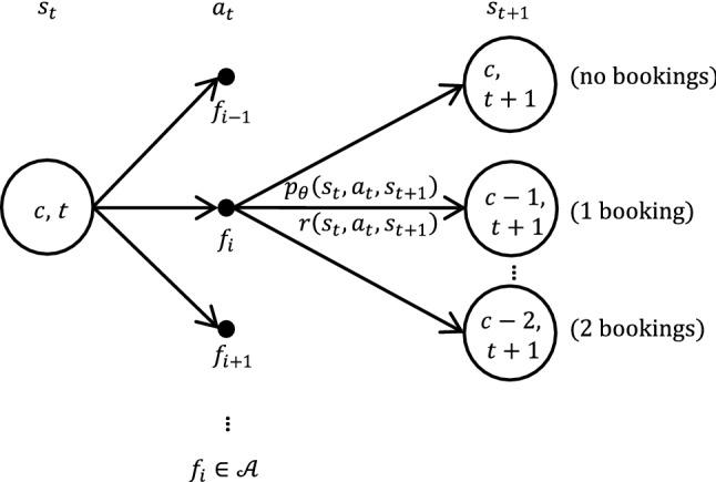
Single resource MDP back-up diagram. The system is initially in state $s_t$. The agent chooses an action $a_t$ that causes the system to transition with probability $p_{\theta }\left(s_t,,,a_t,,,s_{t+1}\right)$ into a reachable subsequent state $s_{t+1}$, yielding a reward $r\left(s_t,,,a_t,,,s_{t+1}\right).$

The objective of the agent is to select the optimal policy ${\pi }^{\ast }(s_t)$ that maximizes the expectation of the sum of future rewards until departure, $v^{\ast }\left(s_t\right)={\mathbb{E}}_{{\pi }^{\ast }}\left[{\sum }_{k=t}^{T-1},r_k\right]$. The optimal policy can be extracted from the state-action value function $q^{\ast }\left(s_t,,,a_t\right)$ which is the revenue to go from state $s_t$, given the agent takes an action $a_t$ and then acts following the optimal policy until termination. The Dynamic Program for the state-action value function and its relation to the value function $v^{\ast }\left(s_t\right)$ is given below.

$$q^{\ast }\left(s_t,,,a_t\right)=\sum _{s_{t+1}\in \mathcal{S}}{p}_{\theta }\left(s_t,,,a_t,,,s_{t+1}\right)\times \left[r,\left(s_t,,,a_t,,,s_{t+1}\right),+,\underset{a_{t+1}}{\max },,q^{\ast },\left(s_{t+1},,,a_{t+1}\right)\right],$$

where $s_t\in \mathcal{S},a_t\in \mathcal{A},$ and $t=0,\dots ,T-1.$ The optimal state value function $v^{\ast }\left(s_t\right)={\max }_{a_t}{q}^{\ast }\left(s_t,,,a_t\right)$ is given employing the revenue maximizing action ${\pi }^{\ast }\left(s_t\right)={\mathrm{argmax}}_{a_t}{q}^{\ast }\left(s_t,,,a_t\right)$.

Anatomy of a demand shock

We define a trajectory as the path a flight takes through state-action space. Hence, a trajectory is a sequence of state-action pairs which records the offered prices and the subsequent bookings received in each time step $t$. Once a trajectory reaches its terminal state $s_T$, the flight departs. Note that we omit the rewards in our definition of the trajectory, since in our setting there is a deterministic reward of moving from one state $s_t$ to the successor state $s_{t+1}$: namely, $r_t=(c_t-c_{t+1})a_t$, where $c_t-c_{t+1}$ is the change in remaining capacity.

While a trajectory represents the path of a single flight through state-action space, it is also of interest to consider a collection of multiple trajectories—for example, multiple departure dates of a flight that departs once per day. We define the departure horizon $1,\dots ,T_{\text{dep}}$ as the set of departure dates (indexed by days to departure) for active flights, where $T_{\text{dep}}$ is the furthest active departure date from today’s date (e.g., $T_{\text{dep}}=365$ if flights are available for sale one year out).

In the remainder of the paper, and without loss of generality, we assume for ease of exposition that the booking horizon and departure horizon have the same cardinality ($T=T_{\text{dep}}$), and that the time step is one day.

We define a trajectory set $\mathcal{J}$ as a set of one or more trajectories , $i=1,\dots ,N$ where $N$ is the cardinality of the trajectory set. The departure date of trajectory is denoted $t_{\text{dep}}\left(i\right),$ where $t_{\text{dep}}:\{1,\dots ,N\}\to \{1,\dots ,T_{\text{dep}}\}$. This notation allows us to represent any flight schedule or aggregation of multiple flights per departure day in the trajectory set$.$

The triangle in Fig. 2 illustrates a trajectory set containing a total of $T_{\text{dep}}$ future departure dates (e.g., one year). The horizontal axis indexes the departure horizon (departure dates) and the vertical axis indexes the booking horizon (time steps). Each trajectory (active flight) in the trajectory set can be represented as a vertical line in the triangle; one such trajectory , representing a flight that departs in 65 days from now, is illustrated in the figure.

Fig. 2.

Two-dimensional time aspects of RMS historic database for a given flight. The triangle contains live sales data. Prior to the shock, the data are generated according to the pre-shock parameters, while after the shock (represented by the diagonal line) the data are generated according to the post-shock parameters

We consider a demand shock that simultaneously affects the entire trajectory set as follows: prior to the demand shock, the state transition probabilities for all trajectories are governed by a vector of pre-shock demand parameters ${\theta }_0=\left({\lambda }_0,,,{\gamma }_0\right)$, which are assumed to be known to the RMS. This region is shown in the dark blue area on the left side of the triangle marked “pre-shock.” After the demand shock, the state transition probabilities for all trajectories are governed by a vector of post-shock demand parameters ${\theta }_1=\left({\lambda }_1,,,{\gamma }_1\right),$ which are unknown to the RMS. This region as shown in the light blue area on the right side of the triangle marked “post-shock.” The demand shock occurs at the separation between the pre-shock and post-shock regions, which is shown as the red diagonal line.

Let ${\tau }_{\text{shock}}$ refer to the number of time steps that have elapsed since the demand shock occurred, which is also unknown to the RMS. Note that ${\tau }_{\text{shock}}$ is not a fixed quantity—it increases with time. At the onset of a shock, ${\tau }_{\text{shock}}=0$. All active flights are not yet impacted by the shock (Fig. 2, the dark blue area covers fully the triangle). As system time progresses, ${\tau }_{\text{shock}}$ increases and more and more of the active flights’ history are impacted by the shock until eventually at ${\tau }_{\text{shock}}=T_{\text{dep}}$ all of the active flight data are generated under the post-shock parameters (Fig. 2, the light blue area covers fully the triangle).

For trajectory , let $t_{\text{shock}}\left(i\right)=T-t_{\text{dep}}(i)-{\tau }_{\text{shock}}$ be the time step at which the demand shock occurred for that trajectory. The state transition probabilities for trajectory are as follows:

$$p_{\theta }\left(s_t,,,a_t,,,s_{t+1}\right)=\left\{\begin{array}{cc}{p}_{{\theta }_0}\left(s_t,,,a_t,,,s_{t+1}\right)& \text{for}t<t_{\text{shock}}\left(i\right)\\ p_{{\theta }_1}\left(s_t,,,a_t,,,s_{t+1}\right)& \text{for}t\ge t_{\text{shock}}\left(i\right)\end{array}\right)$$

As a concrete example, consider the situation where we have one flight per departure day, $T=T_{\text{dep}}=365$, and ${\tau }_{\text{shock}}=100$. For trajectory , $t_{\text{dep}}\left(65\right)=65$ and $t_{\text{shock}}\left(65\right)=200$. Hence, we see that for $t<200$ we follow the pre-shock parameters, while for $t\ge 200$ we follow the post-shock parameters.

Methods for demand change detection

In this section, we provide a framework for detecting demand shocks. This framework provides a science-based approach to detecting anomalous flights in practice, as we will discuss in the section “Practical implementation of the shock detector.”

In this section, we will first assume for the purpose of deriving the statistical properties of the shock detector that the post-shock demand parameters ${\theta }_1=\left({\lambda }_1,,,{\gamma }_1\right)$ are known. Subsequently, we discuss the case of unknown post-shock parameters.

Let ${\mathcal{J}}^{\text{obs}}$ represent an observed trajectory set—the set of active flights for which we wish to detect whether a demand shock has occurred. We construct a hypothesis test for the occurrence of a shock as follows:

$$\begin{array}{ccc}{H}_0:& \theta ={\theta }_0& \forall i,t\end{array}$$

$$\begin{array}{cc}{H}_{{\tau }_{\text{shock}}}:& \left\{\begin{array}{cc}\theta ={\theta }_0& \mathrm{for}t<t_{\text{shock}}\left(i\right)\forall i\\ \theta ={\theta }_1& \mathrm{for}t\ge t_{\text{shock}}\left(i\right)\forall i\end{array}\right)\end{array}$$

Note that the alternative hypothesis is indexed by ${\tau }_{\text{shock}}$, since the time step $t_{\text{shock}}\left(i\right)=T-t_{\text{dep}}(i)-$ ${\tau }_{\text{shock}}$ at which the shock occurs for each trajectory in ${\mathcal{J}}^{\text{obs}}$ is dependent on ${\tau }_{\text{shock}}$.

To test $H_{{\tau }_{\mathit{shock}}}$ against $H_0$, we compute the log likelihood of obtaining the observed trajectory set under each hypothesis. First, we compute the likelihood of observing a single trajectory assuming no shock has occurred while following a deterministic policy $a_t\sim {\pi }^{\ast }\left(s_t\right)$:

Analogously, we compute , the likelihood of a trajectory given a shock that occurred ${\tau }_{\text{shock}}$ time steps ago. Recall that if there is a shock, the state transition probabilities will be governed by demand parameters ${\theta }_0$ until time $t_{\text{shock}}\left(i\right)-1=T-t_{\text{dep}}(i)-{\tau }_{\text{shock}}-1$ and demand parameters ${\theta }_1$ thereafter.

We extend the likelihood computations from single trajectories to the observed trajectory set ${\mathcal{J}}^{\text{obs}}$ by taking the product of likelihood functions over the trajectories in the set:

where we have suppressed the departure day index for readability.

We then compute the likelihood ratio test statistic $D$ (deviance) by comparing the log likelihood of the observed trajectory set under the null hypothesis and under the alternative hypothesis.

$$\frac{D}{2}=\log \frac{{\mathcal{L}}_{\text{shock}}\left({\mathcal{J}}^{\text{obs}}\right)}{{\mathcal{L}}_0\left({\mathcal{J}}^{\text{obs}}\right)}={\ell }_{{\tau }_{\text{shock}}}\left({\mathcal{J}}^{\text{obs}}\right)-{\ell }_0\left({\mathcal{J}}^{\text{obs}}\right),$$

where $\ell \left({\mathcal{J}}^{\text{obs}}\right)=\log \mathcal{L}\left({\mathcal{J}}^{\text{obs}}\right)$ denotes the corresponding log-likelihood function. Large values of the deviance indicate a poor model description and thus lead to a rejection of $H_0.$ To determine the critical region for the deviance, we need to determine its sampling distribution. This can be done in closed form for a simple MDP, as we show below.

Closed form expressions for the log-likelihood functions

Consider again the negative exponential model $d_{\theta }\left(f\right)$, with pre-shock and post-shock parameters ${\theta }_0=\left({\lambda }_0,,,{\gamma }_0\right)$ and ${\theta }_1=\left({\lambda }_1,,,{\gamma }_1\right)$, respectively. Assume no capacity constraining and that the timesteps are sufficiently close that we can ignore multiple bookings in a time step. These assumptions simplify the mathematical derivation, and we will discuss in the section “Shock detection in the general case—parametric bootstrapping” how the framework can be extended in the general case.

Given the simplifying assumptions, we can compute closed form expressions for the log-likelihood functions.

The optimal pre-shock policy in all states is ${\pi }_{{\theta }_0}^{\ast }=f_0/{\gamma }_0$. Let $p_0=d_{{\theta }_0}\left({\pi }_{{\theta }_0}^{\ast }\right)$ and $p_1=d_{{\theta }_1}\left({\pi }_{{\theta }_0}^{\ast }\right)$. The transition probabilities under the pre- and post-shock environments are thus: pre-shock: $p_{{\theta }_0}=p_0$ (booking) and $p_{{\theta }_0}={1-p}_0$ (no booking); post-shock: $p_{{\theta }_1}=p_1$ (booking) and $p_{{\theta }_1}={1-p}_1$ (no booking). Let $n_0$, $n_1$ denote the number of state transitions in the pre-shock and post-shock regions of ${\mathcal{J}}^{\text{obs}}$, respectively, and let $x_0,x_1$ denote the bookings in the pre-shock and post-shock region of ${\mathcal{J}}^{\text{obs}}$, respectively.

The likelihood function ${\mathcal{L}}_{\text{shock}}\left({\mathcal{J}}^{\text{obs}}\right)$ and the corresponding log-likelihood function and its sample distribution can be computed:

$${\mathcal{L}}_{\text{shock}}\left({\mathcal{J}}^{\text{obs}}\right)=p_0^{x_0}{\left(1,-,p_0\right)}^{n_0-x_0}{p}_1^{x_1}{\left(1,-,p_1\right)}^{n_1-x_1}$$

$${\ell }_{\text{shock}}\left({\mathcal{J}}^{\text{obs}}\right)=\sum _{i=0}^1{x}_i\log \left(\frac{p_i}{1-p_i}\right)+n_i\log (1-p_i)$$

Note that this expression for the log-likelihood includes the no-shock log-likelihood as a special case. Indeed, the no-shock case is obtained by setting the post-shock and pre-shock booking probability equal $p_1=p_0.$

Until now we have considered the likelihood of observing a specific set of trajectories. Now we change point of view and focus on the sample distribution of the log-likelihood function. Thus, we consider the log-likelihood function depending on the random variables $X_0$ and $X_1$.

$${\ell }_{\text{shock}}\left({\mathcal{J}}^{\text{obs}}\right)=\sum _{i=0}^1{X}_i\log \left(\frac{p_i}{1-p_i}\right)+n_i\log (1-p_i)$$

Using $X_i\sim \mathrm{Bin}(n_i,p_i)$, $i=0,1$ we can approximate these distributions with Normal distributions. Observe now that the expression for the log-likelihood function is linear of the form $a{X}_0+b{X}_1+c$, where $X_0$ and $X_1$ are normally distributed and $a,b,c$ are constants. Hence, the log-likelihood function also becomes normally distributed ${\ell }_{\text{shock}}\left({\mathcal{J}}^{\text{obs}}\right)\sim N\left({\mu }_{\text{shock}},,,{\sigma }_{\text{shock}}^2\right)$ where

$${\mu }_{\text{shock}}=\sum _{i=0}^1{n}_i{p}_i\log \left(\frac{p_i}{1-p_i}\right)+n_i\log (1-p_i)$$

$${\sigma }_{\text{shock}}^2=\sum _{i=0}^1{n}_i{p}_i\left(1,-,p_i\right){\left(\log ,\left(\frac{p_i}{1-p_i}\right)\right)}^2$$

Similarly, we obtain ${\ell }_0\left({\mathcal{J}}^{\text{obs}}\right)\sim N\left({\mu }_0,,,{\sigma }_0^2\right),$ with

$${\mu }_0=(n_0+n_1)\left[p_0,\log ,\left(\frac{p_0}{1-p_0}\right),+,\log ,(1-p_0)\right]$$

$${\sigma }_0^2=(n_0+n_1)p_0\left(1,-,p_0\right){\left(\log ,\left(\frac{p_0}{1-p_0}\right)\right)}^2$$

Let $m$ be the number of flights per departure day in ${\mathcal{J}}^{\text{obs}}$ (which can also be fractional, e.g., every second day). The sample size becomes $N=m$T, and the total number of state transitions $n_0+n_1=NT/2$, which is the area of the triangle of active flights. Analogously, the number of state transitions in the pre-shock area becomes $n_0=\frac{m{\left(T,-,{\tau }_{\text{shock}}\right)}^2}{2}\approx \frac{\mathit{NT}}{2}-N{\tau }_{\text{shock}}$, and $n_1\approx N{\tau }_{\text{shock}}$ for ${\tau }_{\text{shock}}\ll T$. Note that $n_0,n_1$ and $N$ are integers, thus the relations above are approximations.

$${\mu }_{\text{shock}}-{\mu }_0\approx N{\tau }_{\text{shock}}\times \left[\log ,\left(\frac{1-p_1}{1-p_0}\right),+,p_1,\log ,\left(\frac{p_1}{1-p_1}\right),-,p_0,\log ,\left(\frac{p_0}{1-p_0}\right)\right]$$

Thus, the separation between the two Normal distributions grows proportionally to sample size and time since shock.

$${\sigma }_{\text{shock}}^2\approx {\sigma }_0^2=\frac{\mathit{NT}}{2}{p}_0\left(1,-,p_0\right){\left[\log ,\left(\frac{p_0}{1-p_0}\right)\right]}^2$$

That the variance ${\sigma }_{\text{shock}}^2\approx {\sigma }_0^2$ follows from $n_1\ll n_0$ (assuming ${\tau }_{\text{shock}}\ll T$, which holds for shocks that are detectable within a reasonable time frame of at most a few months). Further, it follows from the above expression that the variance grows proportionally with sample size.

Closed form expressions for the statistical power

In this section, we continue with the simplified analytical model and compute the statistical power of the shock detector. Let $\varphi (x)$ and $\mathrm{\Phi }(x)$ denote the pdf and cdf of the standard Normal distribution. Assume ${\mu }_{\text{shock}}>{\mu }_0$ (similar expressions can be obtained for ${\mu }_{\text{shock}}<{\mu }_0$). We choose a significance level $\alpha$ (one-sided). Let $z_{1-\alpha }={\mathrm{\Phi }}^{-1}\left(1,-,\alpha \right)$ denote the quantile. The acceptance region of the one-sided hypothesis test is shown as the $\left(1,-,\alpha \right)100\%$ confidence interval and the rejection region is correspondingly shown as the complement, as illustrated in Fig. 3.

Fig. 3.

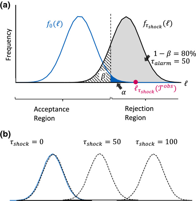
Log-likelihood distributions generated for the null hypothesis $f_0(\ell )$ and the alternative hypothesis $f_{\text{shock}}\left(\ell \right)$ at ${\tau }_{\text{shock}}=50$. Parameters: ${\theta }_0=(\frac{70}{365},0.447)$ and ${\theta }_1=(\frac{70}{365},0.555)$

The power $\mathrm{Pow}$ of the statistical test is the probability of rejection of $H_0$. Hence, the power is computed as the shaded area, c.f. Figure 3 panel (a).

$$\mathrm{Pow}=\mathrm{Pr}({\ell }_{\text{shock}}\left({\mathcal{J}}^{\text{obs}}\right)>{\mu }_0+z_{1-\alpha }{\sigma }_0)={\int }_{{\mu }_0+z_{1-\alpha }{\sigma }_0}^{\infty }\frac{1}{{\sigma }_{\text{shock}}}\varphi \left(\frac{x-{\mu }_{\text{shock}}}{{\sigma }_{\text{shock}}}\right)dx=1-\mathrm{\Phi }\left(\frac{{\mu }_0-{\mu }_{\text{shock}}+z_{1-\alpha }{\sigma }_0}{{\sigma }_{\text{shock}}}\right)$$

Finally, define the alarm time ${\tau }_{\text{alarm}}$ as the expected number of days after a shock at which the statistical power of the detector reaches a given threshold $1-\beta .$

$${\tau }_{\text{alarm}}={\mathrm{argmin}}_{{\mathrm{\tau }}_{\text{shock}}}\left[\mathrm{Pow},\ge ,1,-,\beta \right]$$

To understand how the shock evolves to affect the data over time, see Fig. 3 panel (b), which illustrates how the shock distribution (black dashed curve) propagates from left to right with increasing ${\tau }_{\text{shock}}$. Also shown is the no-shock distribution (blue curve), which remains static.

At the onset of a shock, ${\tau }_{\text{shock}}=0$, ${\mu }_{\text{shock}}={\mu }_0$ and ${\sigma }_{\text{shock}}={\sigma }_0$, and the statistical power $\mathrm{Pow}=\alpha .$ Detection at this point will be entirely random. At the other extreme, ${\tau }_{\text{shock}}=T_{\text{dep}}$, the shock distribution is shifted to the right and the statistical power $\mathrm{Pow}\approx 1,$ which means all shocks will eventually be identified successfully.

In between these two extremes (for example, at ${\tau }_{\text{shock}}=50$), the shock distribution has been shifted such that the statistical power reaches the predefined threshold: $\mathrm{Pow}=1-\beta$. This defines the alarm time.

We can obtain an analytical expression for the alarm time by inverting the power equation employing the relationship $1-\mathrm{\Phi }\left(x\right)=\mathrm{\Phi }\left(-,x\right)$ and inserting the analytical expressions for ${\mu }_{\text{shock}}-{\mu }_0,{\sigma }_{\text{shock}},{\sigma }_0$:

$${\tau }_{\text{alarm}}\approx g(p_0,p_1)\frac{z_{1-\alpha }+{\mathrm{\Phi }}^{-1}\left(1,-,\beta \right)}{\sqrt{N/T}}$$

$$g\left(p_0,,,p_1\right)=\frac{\sqrt{p_0\left(1,-,p_0\right){\left[\log ,\left(\frac{p_0}{1-p_0}\right)\right]}^2/2}}{\left|\log ,\left(\frac{1-p_1}{1-p_0}\right),+,p_1,\log ,\left(\frac{p_1}{1-p_1}\right),-,p_0,\log ,\left(\frac{p_0}{1-p_0}\right)\right|}\approx \frac{\sqrt{p_0\left(1,-,p_0\right)/2}}{|p_1-p_0|}+O{\left(p_1,-,p_0\right)}^0$$

where $g\left(p_0,,,p_1\right)\mathrm{is}\mathrm{a}$ shock scenario-specific factor which depends on the pre-shock booking probability $p_0$ and the post-shock booking probability $p_1$.1 The approximate expression is obtained by a series expansion around $p_0$ to first order.

Thus, we have computed a closed form relationship between alarm time $({\tau }_{\text{alarm}}$), shock scenario-specific factor ($g),$ significance level ($\alpha )$, statistical power ($1-\beta )$, and sample size $(N)$. Below we will discuss their interdependence:

• Shock scenario-specific factor (g

  From the analytical expression, observe that $g\left(p_0,,,p_1\right)$ is a hyperbola where the alarm time is inversely proportional to shock size expressed as $\left|p_1,-,p_0\right|$. This makes intuitive sense. Small shocks will have a high $g\left(p_0,,,p_1\right)$ factor and be hard to detect, while large shocks will have a low $g\left(p_0,,,p_1\right)$ factor and be easy to detect.

• Significance level $$(\alpha)$$(α)

  The significance level $\alpha$ expresses the probability of incorrectly flagging a shock when in fact no shock has occurred (false positive, so-called Type I error). For example, if we choose $\alpha =0.05$, then 5% of flagged shocks will be false alerts. Decreasing the value of $\alpha$ will result in less shocks being flagged, while at the same time also leading to less false positives.

• Statistical power$$\mathbf(1{{-\beta)}}$$(1-β)

  The statistical power expresses the probability of correctly identifying a shock that has occurred. If we choose e.g., $(1-\beta$) = 80%, it implies that given that there has been a shock, we correctly identify 80% of the trajectory sets as having experienced a shock, while we incorrectly classify the remaining 20% as no shock (so-called Type II error). All else equal, increasing the power results in an increase in alarm time.

• Sample size$$\bf(N)$$(N)

  The alarm time scales with the inverse square root of the sample size, which can be used to set the appropriate level of aggregation. Increasing the sample size leads to faster detection but at the same time loses granularity. Therefore, it could be an option to configure multiple shock detectors (possibly overlapping) at various sample sizes and significance levels to detect shocks of different sizes and granularities. For example, the detectors could focus on lower-impact shocks that affect a wide range of markets, or larger-impact shocks affecting a single flight or a single market.

• Alarm time$$\bf({\tau}_{alarm})$$(τalarm)

  The alarm time is the expected time delay before a shock is detected at a specified statistical power. The alarm time depends on the factors discussed and can, for a given shock scenario, be controlled by setting appropriate values for significance level, statistical power, and sample size.

End-to-end shock detection example

In this example, we describe how each of the properties above can be calculated for a specific demand shock. We consider a market AAA-BBB where we have 1 flight per day for one year out, and a one-year booking horizon. Demand arrives following a negative exponential demand model $d_{\theta }\left(f\right)=\mathrm{\lambda }{e}^{-\mathrm{\gamma }\left(f,/,f_0,-,1\right)}$, with pre-shock parameters ${\theta }_0=\left({\lambda }_0,,,{\gamma }_0\right)=$($\frac{70}{365},0.447)$. We will consider the case where a shock has occurred ${\tau }_{\text{shock}}=50$ days ago with post-shock parameters ${\theta }_1=\left({\lambda }_1,,,{\gamma }_1\right)=$($\frac{56}{365},0.447)$, corresponding to a negative shock in the arrival rate of 20%. Using the notation from above, we can summarize:

Known to RMS:

• Sample size: $N=365$

• Pre-shock: ${\theta }_0=(70/365,0.447)\Rightarrow p_0=0.1121$

• Pax expected (no-shock): ${\mathit{NTp}}_0/2=7467$

Unknown to RMS:

• Time since shock: ${\tau }_{\text{shock}}=50$

• Post-shock: ${\theta }_1=(56/365,0.447)\Rightarrow p_1=0.0897$

• Number of state transitions in post-shock region: $n_1=N{\tau }_{\text{shock}}=20440$

• Number of state transitions in pre-shock region: $n_0=\frac{\mathit{NT}}{2}-n_1\approx 46172$

Generation of the trajectory set ${\mathcal{J}}^{\mathit{obs}}$:

Let $Z_i(t)$ be the number of bookings for trajectory at time $t.$ Then $Z_i\left(t\right)$ is Bernoulli distributed with $Z_i\left(t\right)$~$B(p_0)$ for $0\le t<t_{\text{shock}}\left(i\right)$ and $Z_i\left(t\right)$~$B({\widehat{p}}_1)$ for $t_{\text{shock}}\left(i\right)\le t<T-i,$ where $t_{\text{shock}}\left(i\right)=T-t_{\text{dep}}(i)-$ ${\tau }_{\text{shock}}$ as before denotes the separation in time between the pre-shock and post-shock region. Given estimates of post-shock parameters and time since shock ${\widehat{\tau }}_{\text{shock}}$, we compute the number of state transitions $n_1=N{\widehat{\tau }}_{\text{shock}}$, $n_0=\frac{\mathit{NT}}{2}-N{\widehat{\tau }}_{\text{shock}}$ and aggregate the number of bookings in the two regions (which depend on the estimates):

$$\begin{array}{cc}{x}_0={\sum }_{i=1}^T{\sum }_{t=0}^{T-i-{\widehat{\tau }}_{\text{shock}}-1}{z}_i(t),& x_1={\sum }_{i=1}^T{\sum }_{t=T-i-{\widehat{\tau }}_{\text{shock}}}^{T-i-1}{z}_i(t)\end{array}$$

Maximum likelihood estimation:

Inserting these values into ${\ell }_{\text{shock}}\left({\mathcal{J}}^{\text{obs}}\right)$ provides the maximum likelihood estimates (MLE):

$${{{\widehat{\tau }}^{\mathit{MLE}}}_{\text{shock}},{\widehat{\theta }}_1^{\mathit{MLE}}=\mathrm{argmax}}_{{\widehat{\tau }}_{\text{shock}},{\theta }_1}\left({\ell }_{\text{shock}},\left({\mathcal{J}}^{\text{obs}}\right)\right)$$

We assume that the shock has only affected the demand volume (i.e., ${\gamma }_1={\gamma }_0$), the reason being that we are unable to estimate the price elasticity parameter because we generated all data with constant price, corresponding to the optimal price without capacity constraining, and for simplicity, we drop the “MLE” superscript.

Observations and estimations:

• Observed total bookings: $x_0+x_1=7146$

• Current impact: $2(x_0+x_1)/(p_{0}NT)-1=-4.3\%$

• MLE post-shock: ${\widehat{\theta }}_1=(57.05/365,0.447)\Rightarrow {\widehat{p}}_1=0.0914$

• MLE volume impact: $(57.05-70)/70=-18.5\%$

• MLE time since shock: ${\widehat{\tau }}_{\text{shock}}=56$

Shock detection computations:

• Shock specific factor: $g\left(p_0,,,{\widehat{p}}_1\right)\approx 10.76$

• p-value $<{10}^{-4}$ (probability of no shock—Type I error)

• Power: $\left(1,-,\beta \right)=\mathrm{\Phi }\left({\widehat{\tau }}_{\text{shock}},\sqrt{N/T},/,g,\left(p_0,,,{\widehat{p}}_1\right),-,z_{1-\alpha }\right)=99.9\%$ for $\alpha =0.01$

• Alarm time: ${\tau }_{\text{alarm}}=34$ days (for $\alpha =0.01$, $1-\beta =0.8$)

To summarize, applying the shock detection framework, we have estimated that a demand shock occurred ${\widehat{\tau }}_{\text{shock}}=56$ days ago, causing a volume impact of $-18.5\%$ compared to the pre-shock parameters. Since the shock has not fully propagated across all days to departure, we observe only a $-4.3\%$ reduction in bookings compared to expectations. This information allows the airline analyst to proactively adjust the demand forecast in line with the customer behavior after the demand shock.

Finally, to compare with methods currently used in the industry, we compute the time to shock detection if we were to alert flights individually. Using the same pre-shock and post-shock parameters and inserting $N=1,$ it would take one year (${\tau }_{\text{alarm}}=365$ days) to reach a power of $1-\beta \approx 0.8$ at $\alpha =0.1$. If we instead use the entire trajectory set of $N=365$ flights, as done in the example above, we can detect the shock in ${\tau }_{\text{alarm}}=34$ days with the same statistical power at a much stronger significance level ($\alpha =0.01$), providing both significantly faster time to detection and improved accuracy.

Shock detection in the general case—parametric bootstrapping

The analytical results in the previous sections made two important assumptions: that the state transition probabilities are state independent and that at most one booking occurred at each time step. When the transition probabilities are state dependent (that is, the offered price depends on the state) and multiple arrivals can occur in a time step, we can no longer express the sample distribution in closed form. In this case, we use parametric bootstrapping (Efron and Tibshirani 1986) to construct the log-likelihood sample distribution used in the shock detector.

To perform the bootstrapping, we create an ensemble of independent “virtual copies” $\{{\mathcal{J}}^1,\dots ,{\mathcal{J}}^K\}$ of the observed trajectory set ${\mathcal{J}}^{\text{obs}}$. Each virtual copy matches the dimensions (departure dates, booking horizon, cardinality) of ${\mathcal{J}}^{\text{obs}}$, and is initialized empty. For each virtual copy ${\mathcal{J}}^k,$ trajectories are then generated by following a random walk through state-action space assuming the a priori (pre-shock) demand parameters and the RMS policy ${\pi }_{{\theta }_0}^{\ast }$, which is constructed from solving the Dynamic Program as described previously.

We then compute observations ${{\ell }_k=\ell }_0\left({\mathcal{J}}^k\right)$ of the log-likelihood function for each trajectory set ${\mathcal{J}}^k\in \{{\mathcal{J}}^1,\dots ,{\mathcal{J}}^K\}$ using the state transition probabilities corresponding to the no-shock case. Let $f_0(\ell )$ denote the “empirical” probability distribution functions (epdf) obtained from the ensemble (not to be confused with fare levels, that are also denoted by $f$). Analogously, we compute the epdf for the post-shock demand parameters, which we denote $f_{\text{shock}}(\ell )$. We will return to these distributions below, and in Fig. 4.

Fig. 4.

Log-likelihood sample distributions for the analytical model and parametric bootstrapping shock detectors for ${\tau }_{\text{shock}}=0$ and ${\tau }_{\text{shock}}=50$. Parameters: ${\theta }_0=(\frac{70}{365},0.447)$ and ${\theta }_1=(\frac{70}{365},0.555)$

Further let $F_0(\ell )$ denote the corresponding empirical cumulative distribution function (ecdf). In this way, the ensemble produces a sample distribution of the log-likelihood function. As before, we determine the acceptance region of the one-sided hypothesis test as the $\left(1,-,\alpha \right)100\%$ confidence interval $]-\infty ,F_0^{-1}(1-\alpha )]$ from the sample distribution $F_0(\ell )$.

To perform the hypothesis test, we evaluate the log likelihood, ${\ell }_0\left({\mathcal{J}}^{\text{obs}}\right)$ of the observed trajectory set ${\mathcal{J}}^{\text{obs}}$ for the active flights. If ${\ell }_0\left({\mathcal{J}}^{\text{obs}}\right)$ falls outside of the acceptance region, we reject the null hypothesis and flag that a demand shock has occurred.

In the section “Closed form expressions for the log-likelihood functions,” we determined closed form expressions for the log-likelihood sample distribution ${\ell }_0\sim N\left({\mu }_0,,,{\sigma }_0^2\right),$ and ${\ell }_{\text{shock}}\sim N\left({\mu }_{\text{shock}},,,{\sigma }_{\text{shock}}^2\right),$ for the pre- and post-shock distributions, respectively. These normally distributed pdfs can be compared to the corresponding epdfs $f_0(\ell )$ and $f_{\text{shock}}(\ell )$ obtained using parametric bootstrapping, as explained above.

Figure 4 shows one such example of comparing the pdfs (analytical model) and epdfs (parametric bootstrapping), under identical demand parameters at ${\tau }_{\text{shock}}=0$ and ${\tau }_{\text{shock}}=50$. Note that the distributions from the analytical model are shifted with respect to the empirical distributions due to the differences in demand assumptions. This offset implies that we cannot rely solely on the analytical model to determine the critical regions.

Importantly, however, the offset between the pdf and the epdf appears to be constant independent of demand parameters in the considered scenario and with the assumptions made so far. This also means that the deviance metric that measures the difference between the log-likelihood functions under the pre-shock and post-shock demand parameters (i.e., the difference between the two epdfs) can accurately be approximated using the analytical model (i.e., the difference between the two pdfs). This implies that even though we cannot use the analytical model to construct explicit values for the critical regions, we can trust the analytical closed form expression for the power (because it relies only on the difference between the no-shock and shock distributions), without having to resort to an entirely simulation-based approach.

Simulation studies

In this section, we validate the theoretical properties of the shock detector. We construct a simulation environment in which bookings arrive according to a specified pre-shock demand model until a demand shock occurs at a predetermined time. Both the shock impact and the time since shock are unknown to the detector. We then measure the number of days necessary for the detector to identify the shock. For each scenario, the shock detection performance computed using the analytical model is included for reference.

In our simulation environment, we retain the fenceless fare structure, capacity, and negative exponential demand model from previous sections while representing the willingness-to-pay parameter $\gamma$ in terms of the more widely used business term $frat5=1+\log \left(2\right)/\gamma$. The $frat5$ represents the ratio of the lowest fare at which half of the demand will buy up (Belobaba and Hopperstad 2004). The underlying pre-shock demand parameters are ${\theta }_0=\left({\lambda }_0,,,f,r,a,t,5_0\right)=\left(\frac{70}{365},,,2.55\right)$, which under the optimal policy ${\pi }_0^{\ast }$ produces an expected load factor of 82%.

We evaluate the performance of the detector under various positive and negative shocks in demand volume and willingness-to-pay, which are shown in Table 2. We use a trajectory set ${\mathcal{J}}^{\text{obs}}$ consisting of $N=365$ flights. We set the confidence level to 96% ($\alpha =0.04$). Then, we measure the statistical power of the shock detector across 2000 independent simulations. The results are shown in Fig. 5, where the alarm time ${\tau }_{\text{alarm}}$ at which the statistical power reaches 80% is marked for each scenario.

Table 2.

Demand shock scenarios evaluated in the simulation studies

Scenario	Demand shock parameters
	Shock type	${\lambda }_1$	$frat{5}_1$
(a)	Negative	0.192	1.8
(b)	Positive	0.192	3.3
(c)	Negative	0.123	2.55
(d)	Positive	0.260	2.55
(e)	Negative	0.192	1.8
(f)	Both	0.123 to 0.260 (10 steps)	2.55
(g)	Both	0.192	1.8 to 3.3 (10 steps)

Fig. 5.

Statistical power as a function of days since shock ${\tau }_{\text{shock}}$ for the bootstrapped shock detector and analytical model for scenarios (a)–(d) from Table 2

Overall, we see that the statistical power exhibits an S-shape evolution from a power level of $\mathrm{Pow}\left({\tau }_{\text{shock}},=,0\right)=\alpha$ to $\mathrm{Pow}\left({\tau }_{\text{shock}},=,100\right)\approx 1$. This behavior can intuitively be observed by looking at the overlap between the underlying no-shock and shock distributions at various ${\tau }_{\text{shock}}$ shown for scenario (c).

As predicted in the section “Shock detection in the general case—parametric bootstrapping” the analytical closed form expression for the statistical power provides a very accurate approximation of the power of the detector, even though the demand assumptions differ between the two models. We also observe that negative shocks in demand volume and willingness-to-pay can be detected more quickly than positive shocks. For example, in scenario (a), a negative shock in willingness-to-pay can be detected in about two weeks with 80% power, while an equivalent positive shock in scenario (b) takes one month to detect. This is because a negative shock in willingness-to-pay will result in a sudden loss of bookings received at higher price points, which is easier for the detector to identify compared to the slight increase of bookings associated with a positive shock in willingness-to-pay.

Next, in Fig. 6, we investigate the sensitivity of the shock detector with respect to the number of flights in the trajectory set$.$ For simplicity, we assume that fight schedules are equally spaced across the year (for example, a departure once a week, twice a week, etc.).

Fig. 6.

Average days to detection, ${\tau }_{\text{alarm}}$ estimated from when the statistical power of the test reaches 80%: $1-\beta ({\tau }_{\text{alarm}})=0.8$ as a function of number of flights in the trajectory set for scenario (e)

Adding more flights dramatically improves performance of the detector, and the scaling law ${\tau }_{\text{alarm}}\propto 1/\sqrt{N}$ proven by the analytical model can clearly be seen in Fig. 6. Note again that the analytical model provides an accurate description of the power of the detector as a function of sample size, although the analytical model predicts a slightly faster shock detection than is realized by the detector.

For our last experiment, we study how ${\tau }_{\text{alarm}}$ varies with the intensity of the shock. We evaluate five positive and five negative shocks with different intensities for both volume and willingness-to-pay. Figure 7 presents the findings.

Fig. 7.

Average days to detection, ${\tau }_{\text{alarm}}$ estimated from when the statistical power of the test reaches 80%: $1-\beta ({\tau }_{\text{alarm}})=0.8$ as a function of shock intensity for scenarios (f) and (g)

The pre-shock settings are shown at the center of each chart's horizontal axis. The region to the right of the center line shows positive shocks of increasing intensity, and the region to the left shows negative shocks of increasing intensity. The alarm time ${\tau }_{\text{alarm}}$ is shown in the left axis of each panel. Again, the analytical model closely approximates the performance of the detector in all shock scenarios. Furthermore, as shocks get more extreme, the less time it takes to detect them.

Practical implementation of the shock detector

In this section, we discuss how the theoretical shock detector mechanism described in previous sections could be used in practice via an alert center application in an RMS. Figure 8 shows how the shock detector can be integrated into a typical RMS process flow of demand forecasting, optimization and availability control.

Fig. 8.

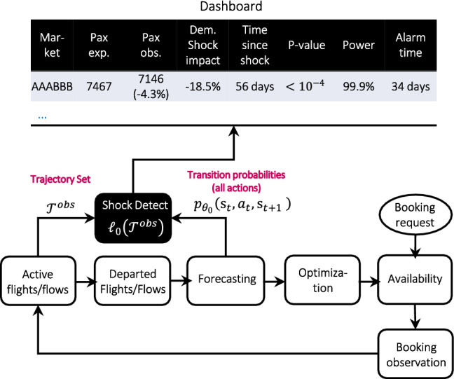
Implementation of shock detection in practice

Following the flow in Fig. 8, incoming bookings and RMS controls (i.e., offered prices for active flights) are stored in the active flight/flow database. Note that RMS controls are stored even if no bookings are observed. Once a flight departs, it moves from the live flight/flow database to the departed flight/flow database. These data are used by the forecasting module, which estimates the forecast parameters and computes the demand forecasts for all possible control policies (Fiig et al. 2014). Finally, the optimization module calculates bid prices used in the availability calculation to determine the RMS controls.

The input data for the shock detection algorithm—the trajectory set ${\mathcal{J}}^{\text{obs}}$—can be compiled from the active flight database and the forecasting module. This corresponds to the transition probabilities $p_{\theta }\left({\mathrm{s}}_t,,,a_t,,,{\mathrm{s}}_{t+1}\right)$ that are used to compute the observed value of the log-likelihood function assuming no shock ${\ell }_0\left({\mathcal{J}}^{\text{obs}}\right)$. As discussed in the section “Shock detection in the general case—parametric bootstrapping,” we can then employ parametric bootstrapping to construct the empirical distribution function $F_0(\ell )$, which is used to construct acceptance and rejection regions used to detect a shock affecting ${\mathcal{J}}^{\text{obs}}$.

The data produced from the demand shock detection mechanism could be used as part of an alert center dashboard to draw the analyst’s attention to aggregations of flights that have experienced a demand shock. The alert center would operate as an offline process that daily or weekly scans the airline’s entire network to provide lists of O&D markets, regions, or other aggregations of flights that experienced a shock. The shock detector can be configured through a variety of criteria—for example, the shock impact or Type I and Type II error levels—to alert users to shocks with significant business relevance while limiting the number of false alerts.

The shock detector can also generate additional KPIs to display along with the list of markets or other aggregations that have experienced a shock. In Fig. 8, we have illustrated some of this information, such as the demand shock impact, time since shock, expected bookings, observed bookings, p-value, and statistical power, following the End-to-end shock detection example presented previously.

Such information would allow airline analysts to sort and rank shocks in order of recency or revenue impact, allowing analysts to prioritize their shock investigation and decide on corrective actions. In this example where the shock detector has identified an 18% reduction in demand volume, the analyst may choose to apply an intervention to lower the demand forecast for future flights in the market, to ensure that the RMS does not overprotect capacity.

Extensions and future work

In this paper, we have made several simplifying assumptions for ease of exposition. For example, we have formulated the detection methodology for a single flights or multiple flights, but not across O&D markets. However, the concepts and methodologies generalize easily to the O&D market level. The transition probabilities at the traffic flow level are one of the byproducts of a conditional demand forecast (Fiig et al. 2014) which the airline would already have computed in order to perform the network optimization. The offered prices (actions) for each traffic flow are also available from the historical booking data for the trajectory. The shock detector would then simply use the relevant transition probabilities and offered prices associated with each traffic flow when computing the log likelihood of a trajectory, and when generating the trajectories used in parameter bootstrapping.

Additionally, there are several avenues of future work that could be explored to improve the performance of the shock detector. First, the speed of shock detection could be further improved from the method presented here. One possibility would be to apply a weight decay to the state transition probabilities $p_{\theta }(s_t,a_t,s_{t+1})$ such that more recent observations are weighted more in the calculation of the log-likelihood function. Alternatively, the shock detection mechanisms could focus on transitions from only the most recent sales dates, as opposed to the set of all transitions in the trajectory set. Such an idea has recently been successfully applied to adapt the RMS forecast to widespread demand changes caused by the COVID-19 pandemic (Fiig et al. 2020).

Finally, we have shown that the analytical model well represents the performance of the bootstrapped shock detector in a case with a simple demand model. It is also worth investigating whether these properties continue to hold in more complex cases, including across multiple fare families and time-dependent demand volumes or willingness-to-pay.

Conclusions

Sudden, unobservable changes in customer behavior can create significant demand forecast error, which can be costly to airlines. Identifying these demand shocks can be a time-consuming process for airline analysts, who often set arbitrary performance thresholds to flag flights or markets with abnormal booking behavior. Analysts often struggle to determine appropriate thresholds to accurately identify meaningful demand shocks while limiting the amount of false positive alerts.

In this paper, we introduced a science-based framework for demand shock detection. Our shock detector computes the log likelihood that a set of active flights followed the observed trajectories in state-action space, assuming that demand was governed by the pre-shock forecast parameters. If the log likelihood of the trajectory set falls outside an acceptance region, this indicates a poor model description by the forecast parameters and thus leads to the conclusion that a shock has occurred.

We demonstrated how with simple state-independent transition probabilities, we could analytically compute a closed form relationship between alarm time $({\tau }_{\text{alarm}}$), shock scenario-specific factor ($g$), significance level ($\alpha )$, statistical power ($1-\beta )$, and sample size $(N)$. For more complex environments with state-dependent transition probabilities, we demonstrated how a parametric bootstrapping approach could be used to construct the acceptance region for the shock detector. We found through simulations that the shock detector exhibited the expected statistical properties and was well described by the analytical model.

We described how our framework could be integrated into an RMS and used to display an estimate of shock impact and time since shock to airline analysts in an alert center application, allowing the airline analyst to easily and quickly identify shocks and prioritize them. This limits the burden on airline analysts and allows them to focus their energy on responding to changes in demand, rather than on merely identifying such changes.

Biographies

Giovanni Gatti Pinheiro

is a Ph.D. student in Reinforcement Learning applied to Revenue Management in the University of Nice Sophia-Antipolis.

Thomas Fiig

is a Director, Chief Scientist at Amadeus, where he is responsible for revenue management strategy and scientific methodologies. He holds a Ph.D. in Theoretical Physics and Mathematics and a BA in Finance from the University of Copenhagen, Denmark. He has published several articles, recently focused on methodologies for origin-and-destination forecasting and optimization of simplified fare structures and dynamic pricing.

Michael D. Wittman

is an Expert, Revenue Management Science & Research at Amadeus, where he works on developing new models for forecasting and optimization in revenue management and dynamic pricing. He holds a Ph.D. in Air Transportation Systems from MIT and is the author of a dozen articles published in peer-reviewed academic journals. His work has won awards and recognition from AGIFORS and INFORMS.

Michael Defoin-Platel

is a Head of Machine Learning Services at Amadeus. He received a Ph.D. in Artificial Intelligence from the University of Nice. He has been conducting academic research in fundamental and applied AI during 10 years before moving to the industry. He is now responsible for the development of AI in Amadeus products.

Riccardo D. Jadanza

is a Head of Artificial Intelligence Research, leader and coordinator of the data scientist “Brain” team at Enerbrain, where he works mainly on studying, developing, and implementing Machine Learning techniques for energy management optimization in HVAC systems in all kinds of buildings. He holds a Ph.D. in Mathematics from the Polytechnic University of Torino and has previously worked in the field of Complex Systems and in the Revenue Management division at Amadeus.

References

- Aviv Y, Pazgal A. A partially observed markov decision process for dynamic pricing. Management Science. 2005;51(9):1400–1416. doi: 10.1287/mnsc.1050.0393. [DOI] [Google Scholar]
- Basseville, M. and I.V. Nikoforov. 1993. Detection of Abrupt Changes. Prentice Hall.
- Belobaba, P.P. and C. Hopperstad. 2004. Algorithms for revenue management in unrestricted fare markets. In Proceedings of the INFORMS section on revenue management, Cambridge, MA.
- Besbes O, Sauré D. Dynamic pricing strategies in the presence of demand shifts. Manufacturing & Operations Service Management. 2014;16(4):513–528. doi: 10.1287/msom.2014.0489. [DOI] [Google Scholar]
- Besbes O, Zeevi A. On the minimax complexity of pricing in a changing environment. Operations Research. 2011;59(1):66–79. doi: 10.1287/opre.1100.0867. [DOI] [Google Scholar]
- Broder J, Rusmevichientong P. Dynamic pricing under a general parametric choice model. Operations Research. 2012;60(4):965–980. doi: 10.1287/opre.1120.1057. [DOI] [Google Scholar]
- den Boer AV. Tracking the market: Dynamic pricing and learning in a changing environment. European Journal of Operational Research. 2015;247:914–927. doi: 10.1016/j.ejor.2015.06.059. [DOI] [Google Scholar]
- den Boer AV, Keskin NB. Discontinuous demand functions: Estimation and pricing. Management Science. 2020;66(10):4516–4534. doi: 10.1287/mnsc.2019.3446. [DOI] [Google Scholar]
- Efron B, Tibshirani R. Bootstrap method for standard errors, confidence intervals, and other measures of statistical accuracy. Statistical Science. 1986;1(1):54–77. [Google Scholar]
- Fiig T, Isler K, Hopperstad C, Belobaba P. Optimization of mixed fare structures: Theory and applications. Journal of Revenue and Pricing Management. 2010;9(1):152–170. doi: 10.1057/rpm.2009.18. [DOI] [Google Scholar]
- Fiig T, Härdling R, Pölt S, Hopperstad C. Demand forecasting and measuring forecast accuracy in general fare structures. Journal of Revenue and Pricing Management. 2014;13(6):413–439. doi: 10.1057/rpm.2014.29. [DOI] [Google Scholar]
- Fiig T, Weatherford LR, Wittman MD. Can demand forecast accuracy be linked to airline revenue? Journal of Revenue and Pricing Management. 2019;18(4):291–305. doi: 10.1057/s41272-018-00174-2. [DOI] [Google Scholar]
- Fiig, T., M.D. Wittman, L. Andersen, C. Föcker, R. Härdling, T. Tofteby, C. Trescases, and L. Zannier. 2020. Revenue management forecasting in times of change: Addressing the need for speed. Presented at the 2020 AGIFORS annual symposium.
- Gallego G, van Ryzin G. Optimal dynamic pricing of inventories with stochastic demand over finite horizons. Management Science. 1994;40(8):999–1020. doi: 10.1287/mnsc.40.8.999. [DOI] [Google Scholar]
- Garivier, A., and E. Moulines. 2011. On upper-confidence bound policies for switching Bandit problems. In ALT 2011: Algorithmic Learning Theory, 174–188.
- Hadoux, E., A. Beynier, and P. Weng. 2014. Sequential decision-making under non-stationary environments via sequential change-point detection. In Proceedings of the 2014 learning over multiple contexts (LMCE), Nancy, France, 1–13.
- Keller G, Rady A. Optimal experimentation in a changing environment. The Review of Economic Studies. 1999;66(3):475–507. doi: 10.1111/1467-937X.00095. [DOI] [Google Scholar]
- Keskin NB, Zeevi A. Chasing demand: Learning and earning in a changing environment. Mathematics of Operations Research. 2017;42(2):277–307. doi: 10.1287/moor.2016.0807. [DOI] [Google Scholar]
- Lai TL. Sequential changepoint detection in quality control and dynamical systems. Journal of the Royal Statistical Society B. 1995;57(4):613–644. [Google Scholar]
- Talluri KT, van Ryzin GJ. The theory and practice of revenue management. New York: Springer; 2005. [Google Scholar]
- Vinod B. An approach to adaptive robust revenue management with continuous demand management in a COVID-19 era. Journal of Revenue and Pricing Management. 2021;20(1):10–14. doi: 10.1057/s41272-020-00269-9. [DOI] [Google Scholar]
- Weatherford L. Performance of dynamic user influence strategies in PODS under seasonality and system volatility. Journal of Revenue and Pricing Management. 2019;18:2–26. doi: 10.1057/s41272-017-0135-8. [DOI] [Google Scholar]