A Fractional-Order Epidemic Model with Quarantine Class and Nonmonotonic Incidence: Modeling and Simulations

Abstract

In any outbreak of infectious disease, the timely quarantine of infected individuals along with preventive measures strategy are the crucial methods to control new infections in the population. Therefore, this study aims to provide a novel fractional Caputo derivative-based susceptible-infected-quarantined-recovered-susceptible epidemic mathematical model along with a nonmonotonic incidence rate of infection. A new quarantined individual compartment is incorporated into the susceptible-infected-recovered-susceptible compartmental model by dividing the total population into four subpopulations. The nonmonotonic incidence rate of infection is considered as Monod–Haldane functional type to understand the psychological effects in the population. Qualitative analysis of the study shows that the model solutions are well-posed i.e., they are nonnegative and bounded in an attractive region. It is revealed that the model has two equilibria, namely, disease-free (DFE) and endemic (EE). The stability analysis of equilibria is investigated for local as well as global behaviors. Mathematical analysis of the model reveals that DFE is locally asymptotically stable when the basic reproduction number $(R_0)$ is lower than one. The basic reproduction number $R_0$ is computed using the next-generation matrix method. The existence of EE is shown and it is investigated that EE is locally asymptotically stable when $R_0>1$ under some appropriate conditions. Moreover, the global stability behaviors of DFE and EE are analyzed under some conditions using $R_0$. Finally, some numerical simulations are performed to interpret the theoretical findings.

Introduction

Mathematical models are playing a crucial role in understanding and controlling the spread of infectious diseases since a very long time. Epidemiological researchers have developed numerous models to understand the dynamics of infectious diseases, such as $\mathrm{SIR},\mathrm{SEIR},\mathrm{SIRS},\mathrm{SAIR},\mathrm{SVEIRS},$ and many others (where $S$ stands for susceptible, $A$ for alert, $E$ for Exposed, $V$ for vaccinated, $I$ for Infected, and $R$ for recovered individuals) (Gumel et al. 2006; Goel et al. 2020a, 2020b; Kumar and Nilam 2019; Kumar et al. 2019; Haung et al. 2010; Goel and Nilam 2019; Alexander et al. 2004; Xu and Ma 2009; Wang 2002; Michael et al. 1999; Zhou and Wang 2022). In mathematical epidemiological literature, many studies are based on classical and integer-order derivatives, which are taken as a vital tool for model formulation; for example, see Gumel et al. (2006), Goel et al. (2020a), Kumar and Nilam (2019), Kumar et al. (2019), Alexander et al. (2004) and Wang (2002). In the last few years, researchers are focusing on developing more realistic models using Fractional-order derivatives instead of integer order derivatives which provide more rich dynamics of epidemic models; for example, see Matignon (1996), Rostamy and Mottaghi (2016), Ahmed et al. (2006), Ye and Xu (2019), Khan et al. (2020), Swati (2022), Cui et al. (2022), Chatterjee et al. (2022) and Zhou and Wang (2022).

Fractional calculus is a special branch of mathematics that deals with derivatives of fractional order, unlike the ordinary derivative which is a local operator in nature. The fractional-order derivative has a vital property called the memory effect. As we all know that every biological phenomenon has long-range temporal memory, therefore, the use of the fractional-order derivative in epidemic models instead of the integer-order derivative provides the systems with long-term memory, which has been proven more realistic. There are several definitions of fractional order derivatives (Camargo and Oliveira 2015; Saad et al. 2018). The majorly used definition of fractional order derivative is proposed by Caputo in 1967. Caputo fractional-order derivative-based differential equations system is one of the most used in the field of mathematical modeling. In Caputo derivative-based equation systems, the initial conditions can be expressed in the same manner as in the integer-order based differential equations system. Also, the Caputo fractional derivative has the same property as an integer-order derivative, i.e., the derivative of a constant is zero. This makes the Caputo fractional derivative more popular and useful over other fractional derivatives such as Riemann-Liouville, Grunwald-Letnikov fractional derivatives, etc. Below is the definition and expression of the Caputo fractional order derivative (Lu and Zhu 2018; Ye and Xu 2019):

“The Caputo fractional derivative of order $\alpha$ of a function $f(x)\in C^n\left(\left[x_0,,,+,\infty \right],,,\mathbb{R}\right)$ is defined as

$$D_x^{\alpha }f\left(x\right)=\frac{1}{\mathrm{\Gamma }(n-\alpha )}{\int }_{x_0}^x\frac{f^{\left(n\right)}(\mathrm{\Omega })}{{\left(x,-,\mathrm{\Omega }\right)}^{\alpha +1-n}}d\mathrm{\Omega },$$ 1

where $x_0\ge x,\mathrm{\Gamma }.$ is the Gamma function and $n$ is the positive integer such that $n-1<\alpha \le n$. When $n=1$, $0<\alpha \le 1$, we have.

$$D_x^{\alpha }f\left(x\right)=\frac{1}{\mathrm{\Gamma }(1-\alpha )}{\int }_{x_0}^x\frac{f{}^{\prime }(\mathrm{\Omega })}{{\left(x,-,\mathrm{\Omega }\right)}^{\alpha }}d\mathrm{\Omega }.$$

The spread of any infectious disease mainly depends on the incidence rate. In epidemiology, the number of individuals who become infected per unit of time is known as the incidence rate (Kermack and Mckendrik 1927; Kumar and Nilam 2021; Goel and Nilam 2019). Kermack and McKendrick (1927) introduced the first infectious disease model using a bilinear incidence rate of the form $\beta SI$. This bilinear incidence rate is based on the law of mass action, which is inconsiderable for a large population. Therefore, in lateral years, many researchers have modified this bilinear incidence rate to the nonlinear incidence rates such as the Holling type II, Crowley–Martin functional type, Beddington–DeAngelish functional type, etc., to study the dynamics of infectious diseases for a large population (Kumar et al. 2019; Goel and Nilam 2019; Dubey et al. 2016; Shi et al. 2011; Liu et al. 1987). In 1986 Liu et al. (Liu et al. 1986) suggested a general incidence rate of the form:

$$f\left(S,,,Y\right)=g\left(Y\right)S=\frac{k{Y}^{p}S}{1+\alpha Y^q}$$ 2

In the above expression, $g\left(Y\right)=\frac{k{Y}^p}{1+\alpha Y^q}$ is denoting the nonmonotonic force of infection at the rate $k$, that is, $g\left(Y\right)$ is increasing when $Y$ is small but it is decreasing when $Y$ is large. The incidence rate $f(S,Y)$ can be used to interpret “psychological effects” by susceptibles, i.e., the infection force may get reduced as the number of infected increases for a large number of infected population because in such a situation the number of contacts may tend to reduce for the case $p<q$. The psychological effects can be observed on the general public during the epidemic outbreak of SARS; aggressive measures and policies, such as border screening, mask-wearing, maintaining hygiene, etc., have been proven very effective (Xiao and Ruan 2007) in reducing the infective rate at the later stage of SARS outbreak, even when the number of infective individuals was getting increasing. In Eq. (2) when we consider $p=1\mathrm{and}q=2$ then Eq. (2) reduces to the following form:

$$f\left(S,,,Y\right)=g\left(Y\right)S=\frac{\mathit{kYS}}{1+\alpha Y^2},\mathrm{where}k,\alpha >0.$$ 3

where $\mathit{kY}$ measures the infection force of the disease and $\frac{1}{1+\alpha Y^2}$ describes the psychological effect from the behavioral change of susceptibles when the number of infectives is very high. The parameter $\alpha$ measures the psychological effect of disease on the population when the infective individuals become sufficiently larger in society. The expression of Eq. (3) is a nonmonotonic functional which is also known as the simplified Monod–Haldane incidence rate (Kumar and Nilam 2021).

Whenever an epidemic outbreak emerges, the quarantine of infected people is an effective tool to reduce the spread of the epidemic. Hence, the role of quarantine people cannot be ignored in the spread control of the disease. In this study, to understand the impact of quarantine people, a quarantine class of individuals is introduced into the standard epidemic model for disease transmission dynamics. The word quarantine is simply meant to the situation of forced isolation or some restrictions on the movement of infected individuals to control the disease from spreading further. To reduce the new infection cases among susceptibles, one can quarantine those infectives who have tested positive. In the case of covid-19, quarantined people are those positively tested infected individuals who are staying in a separate room in the household or a repurposed hotel, depending on the severity of infection and risk factors for developing the severity of the disease as per the WHO report (World Health Organization 2021). For the present study, in case of an outbreak of infectious disease, infected individuals who are in hospitals as per the severity of symptoms are also considered as quarantined individuals. In 2002, Hethcote et al. studied the effect of quarantine class with a bilinear incidence rate for infectious disease in six epidemic models. Later, in 2017 Erdem et al., proposed the disease dynamics with the imperfect quarantine of individuals for altering the influenza infection in the population. In our study, it is supposed that quarantined individuals do not mix up with other individuals so they do not infect them, hence, they will not cause further infection in the population, and do help in reducing the incidence rate for new infection cases.

Motivated by the work of Kumar (2020); Michael et al. 1999; Erdem et al. 2017), the proposed work aims to study the effect of nonmonotonic incidence and quarantine class in disease transmission dynamics to achieve adequate understanding in implementing measures to prevent and control infectious diseases among people. For this purpose, a susceptible-infected-recovered-susceptible epidemic compartmental model is extended and proposed by introducing a quarantine class into it. In the model, it is assumed that recovered individuals are having temporary immunity, and with time they will lose the temporal immunity and will become susceptible again. Some infected individuals who are asymptomatic or do not seek medical attention or have not tested positive remain in the infected class for their entire infectious period. Further, it is assumed that some infected individuals move to the recovered class due to the auto-recovery or by adopting alternate therapies other than medical intervention while other infected individuals who have tested positive and seeking sufficient medical attention move into the quarantined class and will remain there until they are no longer infectious and move to recovered class. This paper also aims to provide a new Caputo derivative-based fractional-order susceptible-infected-quarantined-recovered-susceptible epidemic model along with a nonmonotonic incidence rate and its mathematically rich dynamics.

The rest of the paper is structured as follows: in Sect. 2, the fractional-order mathematical epidemic model is proposed, and some of its basic properties are presented. In Sect. 3, the model equilibria and their local stability behaviors are analyzed with the help of threshold value $R_0$. The Global stability behaviors of the model equilibria are investigated using $R_0$ and fractional order Lyapunov function method (Boukhouima et al. 2020) in Sect. 4. In Sect. 5, numerical simulations are performed using Matlab 2012b to validate the analytical studies. Finally, Sect. 6 is dedicated to the discussion, and conclusion of the present study.

Fractional-Order Epidemic Model and Its Properties

This section is devoted to the formulation of a non-integer Caputo derivative-based mathematical epidemic model. For the development of the model, it is assumed that the total population size is $N(t)$. Further, the total population is divided into four subpopulations or classes, namely; susceptible S $(t)$, infected $Y(t)$, quarantine $Q(t),$ and recovered $Z(t)$, respectively. The susceptible class $S(t)$ consists of those individuals who can catch the infection by coming in close contact with infected people. The infected class $Y(t)$ consists of those individuals who have been caught by the infection and can transfer the infection to susceptibles under appropriate conditions. Quarantine class $Q(t)$ consists of those infected people who are tested positive and staying at their homes or hospitalized according to the level of severity of infection. More explanation about quarantine class has mentioned in Sect. 1. Recovered class $Z(t)$ consists of those individuals who have moved from $Y\left(t\right)$ and $Q(t)$ compartments due to auto-recovery and proper medical treatment, respectively. It is assumed that recovered individuals cannot have immunity for a long period, therefore, they can recatch the infection, and hence, they will become susceptible after a certain period. Let $A$ denote the constant recruitment rate of susceptible. Let $\beta$ be the transmission rate of disease among the susceptible population, $\sigma$ be the psychological effect, $\gamma$ be the rate at which recovered individuals move in $S$ compartment. Let $\mu$ be the natural death rate, and parameters $d_1,d_2$ denote the disease-induced mortality rates in $Y$ and $Q$ classes, respectively. The parameters $\omega$, $\theta ,$ and $\delta$ denote the quarantine rate, the auto-recovery rate of infectives, and the recovery rate of quarantined people after medical attention, respectively. Under the above assumptions, the following fractional-order epidemic model is proposed:

$$\left\{\begin{array}{c}\frac{d^{\alpha }S\left(t\right)}{\text{d}{t}^{\alpha }}=A-\mu S-\frac{\beta SY}{1+\sigma Y^2}+\gamma Z,\hfill \\ \frac{d^{\alpha }Y\left(t\right)}{\text{d}{t}^{\alpha }}=\frac{\beta SY}{1+\sigma Y^2}-\left(\mu +d_1+\omega +\theta \right),\hfill \\ \frac{d^{\alpha }Q\left(t\right)}{d{t}^{\alpha }}=\omega Y-\left(\mu +d_2+\delta \right)Q,\hfill \\ \frac{d^{\alpha }Z\left(t\right)}{\text{d}{t}^{\alpha }}=\theta Y+\delta Q-\left(\mu +\gamma \right)Z.\hfill \end{array}\right)$$ 4

Subject to the conditions:

$$S\left(0\right)=S_0>0,Y\left(0\right)=Y_0\ge 0,Q\left(0\right)=Q_0\ge 0,Z\left(0\right)=Z_0\ge 0$$ 5

Here, $\frac{d^{\alpha }}{{\mathit{dt}}^{\alpha }}=D_t^{\alpha }$ is taken in the form of the Caputo derivative of order $\alpha$ such that $0<\alpha \le 1$.

In the proposed model (4), the term $\frac{\beta SY}{1+\sigma Y^2}$ denotes the non-monotonic force of infection at the rate $\beta$.

For biological reasons, all model parameters are supposed to be positive. The list of all variables and parameters of the model (4) is given below in Table 1.

Now, the following lemmas are being provided of the fractional calculus to derive the basic properties of the model (4).

Lemma 1

(Odibat and Shawagfeh 2007), Consider that $\alpha \in (0,1]$ and the functions $f(t)\in C[a,b]$ and its fractional derivative $D_t^{\alpha }f(t)\in C[a,b]$. Then, we get that for all $t\in [a,b]$,

$f\left(t\right)=f\left(a\right)+\frac{1}{\alpha }\frac{d^{\alpha }}{d{t}^{\alpha }}f\left(\xi \right){\left(t,-,a\right)}^{\alpha }$, where $\xi \in [a,t]$.

It is observed that for $\alpha =1$ above Lemma 1reduces to the classical mean value theorem.

Lemma 2

(Podlubny 1999), Consider ${\alpha }_1>0,{\alpha }_2>0$ and $c\in C$. Define $y\left(t\right)=t^{{\alpha }_2-1}{E}_{{\alpha }_1}{,}_{{\alpha }_2}(\pm c{t}^{{\alpha }_1})$, where $E_{{\alpha }_1}{,}_{{\alpha }_2}(z)$ denotes the two-parameter Mittag–Leffler function along with parameters ${\alpha }_1$ and ${\alpha }_2$.Then the Laplace transformation of $y$ is given by

$$\mathcal{L}\left[y,\left(t\right)\right]=\frac{s^{{\alpha }_1-{\alpha }_2}}{s^{{\alpha }_1}\mp c}.$$

Lemma 3

(Podlubny 1999), Assume that ${\alpha }_2$ is an arbitrary real number. If ${\alpha }_1<2$, then there exists a constant $C_E$ such that, for all $z$ in the complex plane,

$$|E_{{\alpha }_1}{,}_{{\alpha }_2}\left(z\right)|\le \frac{{\mathrm{C}}_{\mathrm{E}}}{1+|z|}$$

Now, we state and prove the following theorems for the basic properties of the model (4) below:

Theorem 1

All the solutions of the proposed mathematical epidemic model (4) with initial conditions given by Eq. (5) are non-negative.

Proof

Consider that $S\left(0\right)>0$ at $t=0$. Firstly, we have to prove that $S\left(t\right)\ge 0\forall t\ge 0$. On contrary, assume that $S(t)\ge 0$ is not true. Then, there exists a ${\tau }_1>0$ such that

$$S\left(t\right)=\left\{\begin{array}{cc}>0& if0\le t<{\tau }_1\\ =0& ift={\tau }_1\\ <0& if{\tau }_1<t<{\tau }_1+{ϵ}_1\end{array}\right)$$ 6

where ${ϵ}_1>0$ is assumed sufficiently small. From the first equation of the model (4), we get, ${\left(\frac{d^{\alpha }S\left(t\right)}{d{t}^{\alpha }}\right|}_{t={\tau }_1}=A+\gamma Z>0$. From Lemma 1, for any $0<{ϵ}_1\ll 1$, we have.

$$S\left({\tau }_1,+,{ϵ}_1\right)=S\left({\tau }_1\right)+\frac{1}{\alpha }\frac{d^{\alpha }}{d{t}^{\alpha }}S\left(\xi \right){ϵ}_1^{\alpha }\mathrm{where}{\tau }_1\le \xi \le {\tau }_1+{ϵ}_1$$

consequently, we get $S\left({\tau }_1,+,{ϵ}_1\right)\ge 0$, which is a contradiction of Eq. (6) that $S\left(t\right)<0$ for ${\tau }_1<t<{\tau }_1+{ϵ}_1$. Therefore, we get that $S\left(t\right)\ge 0\forall t\ge 0$.

Next, we have to show that $Q\left(t\right)\ge 0\forall t\ge 0$. Again, we shall complete this by the method of contradiction. Suppose that $Q(t)\ge 0$ is not true. Then, there exists a ${\tau }_2>0$ such that

$$Q\left(t\right)=\left\{\begin{array}{cc}>0& \text{if}0\le t<{\tau }_2\\ =0& \text{if}t={\tau }_2\\ <0& \text{if}{\tau }_2<t<{\tau }_2+{ϵ}_2\end{array}\right)$$ 7

where ${ϵ}_2>0$ is assumed sufficiently small. From the third equation of the proposed model (4), we get, ${\left(\frac{d^{\alpha }Q(t)}{d{t}^{\alpha }}\right|}_{t={\tau }_2}=\omega Y$ > 0. From Lemma 1, for $0<{ϵ}_2\ll 1$, we have.

$$Q\left({\tau }_2,+,{ϵ}_2\right)=Q\left({\tau }_2\right)+\frac{1}{\alpha }\frac{d^{\alpha }}{d{t}^{\alpha }}Q\left(\xi \right){ϵ}_2^{\alpha }\mathrm{where}{\tau }_2\le \xi \le {\tau }_2+{ϵ}_2$$

As a result, we obtain $Q\left({\tau }_2,+,{ϵ}_2\right)\ge 0$, which is a contradiction of Eq. (7) that is $Q\left(t\right)<0$ for ${\tau }_2<t<{\tau }_2+{ϵ}_2$. Therefore, we get that $Q\left(t\right)\ge 0\forall t\ge 0$.

Similarly, we can show that $Y\left(t\right)\ge 0$ and $Z\left(t\right)\ge 0$ for all $t\ge 0$. Therefore, as a consequence, all the solutions $(S\left(t\right),Y\left(t\right),Q\left(t\right),Z\left(t\right))$ of the model (4) with initial conditions (5) are non-negative.

Theorem 2

The region $R=\left\{\left(S,,,Y,,,Q,,,Z\right),\in ,{\mathbb{R}}_{+}^4,:,0,<,S,+,Y,+,Q,+,Z,\le ,\overline{P},,,\overline{P},\ge ,C_E,\frac{A}{\mu }\right\}$ is an attractive region of the model (4), where $C_E$ is a constant described in Lemma 3.

Proof

Adding all the equations of the model (4), we get the following fractional order differential equation:

$$D_t^{\alpha }N=A-\mu N-d_{1}Y-d_{2}Q$$ 8

where $N=S+Y+Q+Z$. Now, as $Y,Q\ge 0$, we get

$$D_t^{\alpha }N\le A-\mu N$$ 9

Now, take the initial value problem

$$D_t^{\alpha }\overline{N}=A-\mu \overline{N},\overline{N}\left(0\right)={\overline{N}}_0$$ 10

From the comparison principle (Lu and Zhu 2018), the solution of Eqs. (9) and (10) satisfy the following inequality:

$$N\left(t\right)\le \overline{N}\left(t\right),\mathrm{for}\mathrm{all}t\ge 0$$ 11

Take the Laplace Transform of Eq. (10), we get

$$\begin{array}{cc}& s^{\alpha }\mathcal{L}[\overline{N}\left(t\right)]-s^{\alpha -1}\overline{N_0}=\frac{A^{\alpha }}{s}-\mu \mathcal{L}[\overline{N}\left(t\right)]\hfill \\ \hfill & \Rightarrow \mathcal{L}\left[\overline{N},\left(t\right)\right]=\frac{s^{\alpha -1}\overline{N_0}}{s^{\alpha }+\mu }+\frac{A^{\alpha }{s}^{-1}}{s^{\alpha }+\mu }\hfill \end{array}$$

Also, from Lemma 2, we get

$$\mathcal{L}\left[E_{\alpha ,1},\left(-,\mu ,t^{\alpha }\right)\right]=\frac{s^{\alpha -1}}{s^{\alpha }+\mu },\mathcal{L}\left[t^{\alpha },E_{\alpha ,\alpha +1},\left(-,\mu ,t^{\alpha }\right)\right]=\frac{s^{-1}}{s^{\alpha }+\mu }.$$

Taking the inverse Laplace transform of the above, we get

$$\overline{N}\left(t\right)=\overline{N_0}{E}_{\alpha ,1}\left(-,\mu ,t^{\alpha }\right)+A{t}^{\alpha }{E}_{\alpha ,\alpha +1}\left(-,\mu ,t^{\alpha }\right)$$

Using Eq. (9), we have

$$N(t)\le N_0{E}_{\alpha ,1}\left(-,\mu ,t^{\alpha }\right)+A{t}^{\alpha }{E}_{\alpha ,\alpha +1}\left(-,\mu ,t^{\alpha }\right)$$

Using Lemma 3, we obtain

$$|N\left(t\right)|\le \frac{N_0{C}_E}{1+\mu t^{\alpha }}+\frac{A{t}^{\alpha }{C}_E}{1+\mu t^{\alpha }}$$

where, $C_E$ is a constant, described in Lemma 3. So, as t $\to \infty$, we obtain $N\left(t\right)\le \stackrel{-}{P,}$ where $\overline{P}\ge C_E\frac{A}{\mu }$.

Therefore, region $R$ is attracting all the solutions $(S(t),Y(t),Q(t),Z(t))$ of the model (4).

Equilibria and Their Stability Analysis

This section is devoted to the existence of the model equilibria and their stability analysis. The model equilibria are obtained by setting all the equations of the model (4) to zero, which are as given below:

• i.Disease-free equilibrium (DFE),$E_1(S_0,Y_0,Q_0,Z_0)=\left(\frac{A}{\mu },,,0,0,,,0\right)$.
• ii.Endemic equilibrium (EE), $E_2=(S^{\ast },Y^{\ast },Q^{\ast },Z^{\ast })$.

A detailed discussion on the existence of endemic equilibrium is given in section 3.3.

To investigate the stability behavior of both equilibria, we need to compute the basic reproduction number $R_0$ (Driessche and Watmough 2002). The basic reproduction number is obtained in Sect. 3.1 using the next-generation matrix method (Driessche and Watmough 2002; Ye and Xu 2019).

Computation of the Basic Reproduction Number ${\mathit{R}}_0$:

For the computation of the basic reproduction number $R_0$, first, we consider that

$$D_t^{\alpha }x=U\left(x\right)-V\left(x\right),$$

where $x$ $={\left(Z,,,Q,,,Y,,,S\right)}^T$, $U(x)$ is the matrix of new infection term and $V(x)$ is the matrix of transfer term into the compartments and out of the compartments. Jacobian matrices of $U(x)$ and $V(x)$ at $E_1$ are given by:

$$U=\left(\begin{array}{cccc}0& 0& 0& 0\\ 0& 0& 0& 0\\ 0& 0& \frac{A\beta }{\mu }& 0\\ 0& 0& 0& 0\end{array}\right),V=\left(\begin{array}{cccc}\gamma +\mu & -\delta & -\theta & 0\\ 0& d_2+\delta +\mu & -\omega & 0\\ 0& 0& d_1+\theta +\mu +\omega & 0\\ -\gamma & 0& \frac{A\beta }{\mu }& \mu \end{array}\right).$$

For the next-generation matrix, we need to calculate the inverse of matrix $V$. The inverse of the matrix $(V^{-1})$ is given in "Appendix A".

Now, the next-generation matrix is:

$$U{V}^{-1}=\left(\begin{array}{cccc}0& 0& 0& 0\\ 0& 0& 0& 0\\ 0& 0& \frac{A\beta (-d_2\gamma \mu -\gamma \delta \mu -d_2{\mu }^2-\gamma {\mu }^2-\delta {\mu }^2-{\mu }^3)}{{\mu }^2(d_2\gamma +\gamma \delta +d_2\mu +\gamma \mu +\delta \mu +{\mu }^2)(-d_1-\theta -\mu -\omega )}& 0\\ 0& 0& 0& 0\end{array}\right)$$

On simplification, we get

$$U{V}^{-1}=\left(\begin{array}{cccc}0& 0& 0& 0\\ 0& 0& 0& 0\\ 0& 0& \frac{A\beta }{\mu (d_1+\theta +\mu +\omega )}& 0\\ 0& 0& 0& 0\end{array}\right)$$

From Ye and Xu (2019), the basic reproduction number is the spectral radius of the next generation matrix $(U{V}^{-1})$ that is denoted by $\rho (U{V}^{-1})$. Hence, the basic reproduction number of the model (4) is:

$$R_0=\rho \left(U,V^{-1}\right)=\frac{A\beta }{\mu (d_1+\theta +\mu +\omega )}=\frac{\beta S_0}{(d_1+\theta +\mu +\omega )}$$ 12

In the above Eq. (12), the term $\frac{1}{d_1+\theta +\mu +\omega }$ denotes the average life expectancy of infectious individuals. The right-hand side term of $R_0$ provides the number of secondary infections of susceptible individuals that one infected individual can produce in a disease-free population.

Further, the local stability behaviors of the equilibrium point $E_1$ of the model (4) are discussed with the help of the basic reproduction number $R_0$.

Local Stability Analysis of Disease-Free Equilibrium (${\mathit{E}}_1$)

The local stability behavior of the disease-free equilibrium of the model (4) can be analyzed by the linearization of the model (4) at the disease-free equilibrium ($E_1)$. Therefore, a linearized matrix of the model (4) is obtained as given below:

$$J=\left(\begin{array}{cccc}-\mu -\frac{Y\beta }{1+Y^2\sigma }& \frac{2S{Y}^2\beta \sigma }{{(1+Y^2\sigma )}^2}-\frac{S\beta }{1+Y^2\sigma }& 0& \gamma \\ \frac{Y\beta }{1+Y^2\sigma }& -d_1-\theta -\mu -\frac{2S{Y}^2\beta \sigma }{{(1+Y^2\sigma )}^2}+\frac{S\beta }{1+Y^2\sigma }-\omega & 0& 0\\ 0& \omega & -d_2-\delta -\mu & 0\\ 0& \theta & \delta & -\gamma -\mu \end{array}\right)$$

From the above, the linearized matrix of the system (4) at DFE ($E_1$)is given as:

$$J_{E_1}=\left(\begin{array}{cccc}-\mu & -\frac{A\beta }{\mu }& 0& \gamma \\ 0& -d_1-\theta +\frac{A\beta }{\mu }-\mu -\omega & 0& 0\\ 0& \omega & -d_2-\delta -\mu & 0\\ 0& \theta & \delta & -\gamma -\mu \end{array}\right)$$

The characteristic equation of the matrix $J_{E_1}$ is as follows:

$$(\lambda +\mu )(\gamma +\lambda +\mu )(d_2+\delta +\lambda +\mu )(-A\beta +\mu (d_1+\theta +\lambda +\mu +\omega ))=0.$$ 13

All characteristic roots of Eq. (13) are given by ${\lambda }_1=-\mu$,${\lambda }_2=-(\mu +\gamma )$, ${\lambda }_3=-(d_2+\delta +\mu )$, ${\lambda }_4=(R_0-1)(d_1+\theta +\mu +\omega )$.

We see that the eigenvalues ${\lambda }_1,{\lambda }_2$ and ${\lambda }_3$ of the matrix $J_{E_1}$ are of with negative sign and the eigenvalue ${\lambda }_4$ will be negative when $R_0<1$. Hence, $|\arg {\lambda }_j|=\pi >\frac{\alpha \pi }{2}$ for all $j=1,2,3,4$.

Now, when$R_0>1$, the eigenvalue${\lambda }_4>0$, and in this situation $|\arg {\lambda }_4|=0<\frac{\alpha \pi }{2}.$ Therefore, the disease-free equilibrium ($E_1)$ is unstable when$R_0>1$. Hence, by Kumar (2020) and Matignon 1996) and the above discussion, we present the following theorem for the local stability behavior of the disease-free equilibrium${(E}_1)$:

Theorem 3

The disease-free equilibrium $E_1=\left(\frac{A}{\mu },,,0,0,,,0\right)$ of the proposed model (4) is:

• i.locally asymptotically stable when the basic reproduction number $R_0<1$.
• ii.unstable when $R_0>1$.

Figure 2 is the graphical representation of Theorem 3 using data as given in Table 2. It confirms that disease will die out when $R_0<1$ and disease will continue its propagation among the population when $R_0>1$.

Fig. 1.

Transfer diagram of the model (4)

Fig. 2.

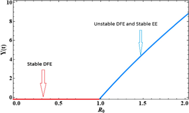
Basic reproduction number $R_0$ versus Infected population $Y(t).$

Table 2.

Parameters and their numerical value

Parameters	$A$	$\mu$	$\beta$	$\sigma$	$\gamma$	$d_1$	$\omega$	$\theta$	$d_2$	$\delta$
Value	9	0.03	0.003	0.002	0.0002	0.04	0.08	0.005	0.04	0.007

Existence of the Endemic Equilibrium (${\mathit{E}}_2)$ and Its Local Stability Analysis

In this section, we present the existence of a unique endemic equilibrium and discuss its local stability behavior. The endemic equilibrium $E_2(S^{\ast },Y^{\ast },Q^{\ast },Z^{\ast })$ of the model is obtained by taking all equations of the model (4) to zero as given below:

$$A-\mu S^{\ast }-\frac{\beta S^{\ast }{Y}^{\ast }}{1+\sigma {Y^{\ast }}^2}+\gamma Z^{\ast }=0,$$

$$\frac{\beta S^{\ast }{Y}^{\ast }}{1+\sigma {Y^{\ast }}^2}-\left(\mu ,+,d_1,+,\omega ,+,\theta \right)Y^{\ast }=0,$$ 14

$$\omega Y^{\ast }-\left(\mu ,+,d_2,+,\delta \right)Q^{\ast }=0,$$

$$\theta Y^{\ast }+\delta Q^{\ast }-\left(\mu ,+,\gamma \right)Z^{\ast }=0.$$

On solving Eq. (14), we get

$$S^{\ast }=\frac{(1+{Y^{\ast }}^2\sigma )(d_1+\theta +\mu +\omega )}{\beta },Q^{\ast }=\frac{Y^{\ast }\omega }{d_2+\delta +\mu },Z^{\ast }=\frac{d_2{Y}^{\ast }\theta +Y^{\ast }\delta \theta +Y^{\ast }\theta \mu +Y^{\ast }\delta \omega }{(\gamma +\mu )(d_2+\delta +\mu )}$$

and $Y^{\ast }$ is the solution of the following quadratic equation:

$$A_2{Y^{\ast }}^2+A_1{Y}^{\ast }+A_0=0$$ 15

where the coefficients $A_0,A_1$ and $A_2$ of Eq. (15) are as given below:

$$\begin{array}{cc}\hfill A_0& =-\left(\gamma ,+,\mu \right)\left(d_2,+,\delta ,+,\mu \right)\left(-,A,\beta ,+,\mu ,\left(d_1,+,\theta ,+,\mu ,+,\omega \right)\right)\hfill \\ \hfill & =(\gamma +\mu )(d_2+\delta +\mu )\mu (d_1+\theta +\mu +\omega )(R_0-1),\hfill \end{array}$$

$$A_1=-\beta \left(d_1,\left(\gamma ,+,\mu \right),\left(d_2,+,\delta ,+,\mu \right),+,d_2,\left(\gamma ,\left(\mu ,+,\omega \right),+,\mu ,\left(\theta ,+,\mu ,+,\omega \right)\right),+,\mu ,\left(\gamma ,\left(\delta ,+,\mu ,+,\omega \right),+,\left(\delta ,+,\mu \right),\left(\theta ,+,\mu ,+,\omega \right)\right)\right),$$

$$A_2=-\mu \left(\gamma ,+,\mu \right)\left(d_2,+,\delta ,+,\mu \right)\sigma \left(d_1,+,\theta ,+,\mu ,+,\omega \right).$$

Now, we state the result in form of the theorem for the existence of a unique positive equilibrium.

Theorem 4

There is at most one positive equilibrium of the model (4) if $R_0>1$.

Proof

Suppose that

$$f\left(Y^{\ast }\right)=A_2{Y^{\ast }}^2+A_1{Y}^{\ast }+A_0=0.$$ 16

The coefficients $A_2$ and $A_1$ of $f(Y^{\ast })$ are negative, and coefficient $A_0$ is positive when $R_0>1$ as all parameters are assumed to be positive. From Eq. (16), it can be seen that $f\left(Y^{\ast }\right)$ is a continuous function in $Y^{\ast }$. Therefore, by Descartes’ Rule of the signs (Wang 2004), there exists at most one real positive root of Eq. (16). Thus, after obtaining the unique positive value of $Y^{\ast }$, we can calculate the value of $S^{\ast },Q^{\ast }$ and $Z^{\ast }$, respectively. Hence, there exists a unique positive endemic equilibrium $E_2=(S^{\ast },Y^{\ast },Q^{\ast },Z^{\ast })$ of the model (4).

Now, the local stability behavior of the endemic equilibrium $E_2=(S^{\ast },Y^{\ast },Q^{\ast },Z^{\ast })$ is investigated.

To investigate the locally asymptotical stability of the endemic equilibrium $E_2$, we need the following lemma:

Lemma 4

(Ahmed et al. 2006; Naik et al. 2020) Define the following characteristic equation:

$$P\left(\zeta \right)={\zeta }^n+a_1{\zeta }^{n-1}+a_2{\zeta }^{n-2}+\cdots +a_n=0$$ 17

The following conditions make all the roots of the characteristics Eq. (17) satisfy the equation given below:

$$|\arg (Eig(J^{\ast }))|=|\arg {\lambda }_j|>\frac{\alpha \pi }{2}\mathrm{for}\mathrm{all}j=1,2,3,4.$$ 18

• i.For $n=1$, the condition for Eq. (17) is $a_1>0$.
• ii.For $n=2$, the conditions for Eq. (17) are either Routh-Hurwitz conditions or $a_1<0,4a_2>a_1^2$, $\left|{\tan }^{-1},(,\sqrt{4a_2-{\left(a_1\right)}^2}\right)/a_1|>\alpha \pi /2$
• iii.
  For $n=3$, if the discriminant of $P\left(\zeta \right)$, namely $D(P)$ is positive, the following conditions are the necessary and sufficient conditions to satisfy Eq. (18):

  $$a_1>0,a_3>0,a_1{a}_2>a_3,\mathrm{if}D\left(P\right)>0$$
• iv.If $D\left(P\right)<0,a_1>0,a_2>0,a_1{a}_2=a_3$ then condition Eq. (18) is satisfied for all $\alpha \in [0,1)$.
• v.For general $n,a_n>0$ is necessary for Eq. (18).

Now, to analyze the local stability behavior of $E_2$, we linearize the model (4) at $E_2$, and obtained the following Jacobian matrix$(J^{\ast })$:

$J^{\ast }=\left(\begin{array}{cccc}-\mu -\frac{Y^{\ast }\beta }{1+{Y^{\ast }}^2\sigma }& \frac{2S{Y^{\ast }}^2\beta \sigma }{{(1+{Y^{\ast }}^2\sigma )}^2}-\frac{S\beta }{1+{Y^{\ast }}^2\sigma }& 0& \gamma \\ \frac{Y^{\ast }\beta }{1+{Y^{\ast }}^2\sigma }& -d_1-\theta -\mu -\frac{2S{Y^{\ast }}^2\beta \sigma }{{(1+{Y^{\ast }}^2\sigma )}^2}+\frac{S\beta }{1+{Y^{\ast }}^2\sigma }-\omega & 0& 0\\ 0& \omega & -d_2-\delta -\mu & 0\\ 0& \theta & \delta & -\gamma -\mu \end{array}\right)$

The characteristic equation of the matrix $J^{\ast }$ is:

$${P\left(\lambda \right)=\lambda }^4+C_3{\lambda }^3+C_2{\lambda }^2+C_1\lambda +C_0=0,$$ 19

where the coefficients $C_0,C_1,C_3$ and $C_4$ are given by:

$$C_0=\frac{1}{1+{Y^{\ast }}^2\sigma }\left(Y^{\ast },(d_1\left(\gamma ,+,\mu \right)\left(d_2,+,\delta ,+,\mu \right)\left(\beta ,+,2,Y^{\ast },\mu ,\sigma \right)+d_2\left(2,Y^{\ast },\mu ,\left(\gamma ,+,\mu \right),\sigma ,\left(\theta ,+,\mu ,+,\omega \right),+,\beta ,\left(\gamma ,\left(\mu ,+,\omega \right),+,\mu ,\left(\theta ,+,\mu ,+,\omega \right)\right)\right)+\mu (2Y^{\ast }(\gamma +\mu )(\delta +\mu )\sigma (\theta +\mu +\omega )+\beta (\gamma (\delta +\mu +\omega )+(\delta +\mu )(\theta +\mu +\omega ))))\right),$$

$$C_1=\frac{1}{1+{Y^{\ast }}^2\sigma }(Y^{\ast }\beta \gamma \delta +Y^{\ast }\beta \delta \theta +2Y^{\ast }\beta \gamma \mu +2Y^{\ast }\beta \delta \mu +\gamma \delta \mu +2Y^{\ast }\beta \theta \mu +3Y^{\ast }\beta {\mu }^2+\gamma {\mu }^2+\delta {\mu }^2+{\mu }^3+2{Y^{\ast }}^2\gamma \delta \theta \sigma +3{Y^{\ast }}^2\gamma \delta \mu \sigma +4{Y^{\ast }}^2\gamma \theta \mu \sigma +4{Y^{\ast }}^2\delta \theta \mu \sigma +5{Y^{\ast }}^2\gamma {\mu }^2\sigma +5{Y^{\ast }}^2\delta {\mu }^2\sigma +6{Y^{\ast }}^2\theta {\mu }^2\sigma +7{Y^{\ast }}^2{\mu }^3\sigma +d_1{Y}^{\ast }(\beta (\gamma +\delta +2\mu )+2Y^{\ast }(\gamma \delta +2\gamma \mu +2\delta \mu +3{\mu }^2)\sigma +d_2(\beta +2Y^{\ast }(\gamma +2\mu )\sigma ))+Y^{\ast }\beta \gamma \omega +Y^{\ast }\beta \delta \omega +2Y^{\ast }\beta \mu \omega +2{Y^{\ast }}^2\gamma \delta \sigma \omega +4{Y^{\ast }}^2\gamma \mu \sigma \omega +4{Y^{\ast }}^2\delta \mu \sigma \omega +6{Y^{\ast }}^2{\mu }^2\sigma \omega +d_2(\mu (\gamma +\mu )+Y^{\ast }\beta (\gamma +\theta +2\mu +\omega )+{Y^{\ast }}^2\sigma (\gamma (2\theta +3\mu +2\omega )+\mu (4\theta +5\mu +4\omega )))),$$

$$C_2=\frac{1}{1+{Y^{\ast }}^2\sigma }\left(Y^{\ast },\beta ,\gamma ,+,Y^{\ast },\beta ,\delta ,+,\gamma ,\delta ,+,Y^{\ast },\beta ,\theta ,+,3,Y^{\ast },\beta ,\mu ,+,2,\gamma ,\mu ,+,2,\delta ,\mu ,+,3,{\mu }^2,+,{Y^{\ast }}^2,\gamma ,\delta ,\sigma ,+,2,{Y^{\ast }}^2,\gamma ,\theta ,\sigma ,+,2,{Y^{\ast }}^2,\delta ,\theta ,\sigma ,+,4,{Y^{\ast }}^2,\gamma ,\mu ,\sigma ,+,4,{Y^{\ast }}^2,\delta ,\mu ,\sigma ,+,6,{Y^{\ast }}^2,\theta ,\mu ,\sigma ,+,9,{Y^{\ast }}^2,{\mu }^2,\sigma ,+,d_1,Y^{\ast },\left(\beta ,+,2,Y^{\ast },\left(d_2,+,\gamma ,+,\delta ,+,3,\mu \right),\sigma \right),+,Y^{\ast },\beta ,\omega ,+,2,{Y^{\ast }}^2,\gamma ,\sigma ,\omega ,+,2,{Y^{\ast }}^2,\delta ,\sigma ,\omega ,+,6,{Y^{\ast }}^2,\mu ,\sigma ,\omega ,+,d_2,\left(Y^{\ast },\beta ,+,\gamma ,+,2,\mu ,+,{Y^{\ast }}^2,\sigma ,\left(\gamma ,+,2,\left(\theta ,+,2,\mu ,+,\omega \right)\right)\right)\right),$$

$$C_3=\frac{1}{1+{Y^{\ast }}^2\sigma }\left(d_2,+,Y^{\ast },\beta ,+,\gamma ,+,\delta ,+,3,\mu ,+,d_2,{Y^{\ast }}^2,\sigma ,+,{Y^{\ast }}^2,\sigma ,(2d_1+\gamma +\delta +2\theta +5\mu +2\omega )\right).$$

All the coefficients $C_0$, $C_1$, $C_2$, $C_3$ of the characteristic Eq. (19) are of positive sign. Thus, from condition (v) of Lemma 4, the unique positive endemic equilibrium $E_2$ is locally asymptotically stable (Ahmed et al. 2006; Naik et al. 2020). Hence, this result is stated in form of the theorem below:

Theorem 5

The endemic equilibrium $E_2=(S^{\ast },Y^{\ast },Q^{\ast },Z^{\ast })$ of the fractional-order epidemic model (4) is locally asymptotically stable when $R_0>1$ and unstable otherwise.

Global Stability Analysis

In this section, we discuss the global stability behavior of the disease-free $\left(E_1\right)$ and endemic equilibria $(E_2)$.

For global stability analysis, we assume that

$$G\left(Y\right)=\frac{Y}{1+\sigma Y^2}.$$ 20

Now, we establish the following theorems corresponding to the global stability behavior of $E_1$ and $E_2$.

Theorem 6

The disease-free equilibrium $E_1=\left(\frac{A}{\mu },,,0,0,,,0\right)$ of the model (4) is globally asymptotically stable when the basic reproduction number is less than or equal to unity, that is, $R_0\le 1$.

Proof

From the system of Eq. (4), we derive the following conditions at $E_1=\left(\frac{A}{\mu },,,0,0,,,0\right)$

$$A=\mu S_0$$

Now, consider the Lyapunov function as:

$$L\left(t\right)=\left(S,-,S_0,-,S_0,l,n,\frac{S}{S_0}\right)+Y+Q+Z,\mathrm{where}{S}_0=\frac{A}{\mu }$$ 21

The differentiation of Eq. (21) along the solution of the model (4) is

$$\begin{array}{cc}\hfill D_t^{\alpha }L\left(t\right)& =\left(1,-,\frac{S_0}{S}\right)D_t^{\alpha }S+D_t^{\alpha }Y+D_t^{\alpha }Q+D_t^{\alpha }Z\hfill \\ \hfill & =\left(1,-,\frac{S_0}{S}\right)\left(A,-,\mu ,S,-,\beta ,S,G,(,Y,),+,\gamma ,Z\right)+\beta SG(Y)-\left(\mu ,+,d_1,+,\omega ,+,\theta \right)Y+\omega Y-\left(\mu ,+,d_2,+,\delta \right)Q+\theta Y+\delta Q-\left(\mu ,+,\gamma \right)Z\hfill \\ \hfill & =\left(1,-,\frac{S_0}{S}\right)(\mu S_0-\mu S-\beta SG\left(Y\right)+\gamma Z+\beta SG(Y)-\left(\mu ,+,d_1,+,\omega ,+,\theta \right)Y+\omega Y-\left(\mu ,+,d_2,+,\delta \right)Q+\theta Y+\delta Q-\left(\mu ,+,\gamma \right)Z\hfill \\ \hfill & =-\mu S{\left(1,-,\frac{S_0}{S}\right)}^2+\beta S_{0}G\left(Y\right)-\left(\frac{\gamma S_0}{S},+,\mu \right)Z-\left(\mu ,+,d_2\right)Q-\left(\mu ,+,d_1,+,\omega ,+,\theta \right)Y+\omega Y+\theta Y\hfill \\ \hfill & \le -\mu S{\left(1,-,\frac{S_0}{S}\right)}^2+\left(\beta ,S_0,-,\left(\mu ,+,d_1,+,\omega ,+,\theta \right)\right)Y-\left(\frac{\gamma S_0}{S},+,\mu \right)Z-\left(\mu ,+,d_2\right)Q+(\omega +\theta )Y(\mathrm{Since}G(Y)\le Y)\hfill \\ \hfill & \le -\frac{\mu {\left(S,-,\frac{A}{\mu }\right)}^2}{S}-\left(\mu ,+,d_1,+,\omega ,+,\theta \right)Y\left(1,-,R_0\right)-\left(\left(\frac{\gamma S_0}{S},+,\mu \right),Z,+,\left(\mu ,+,d_2\right),Q,-,(\omega +\theta ),Y\right).\hfill \end{array}$$

Now from above, it can be observed that if $(\omega$+$\theta )Y\le \left(\frac{\gamma S_0}{S},+,\mu \right)Z+\left(\mu ,+,d_2\right)Q$ and $R_0\le 1$ then $D_t^{\alpha }L(t)\le 0$. In addition, the maximum invariant set in $\{\left(S,,,Y,,,Q,,,Z\right):D_t^{\alpha }L\left(t\right)=0\}$ is the singleton set ${\{E}_1\}$. Therefore, according to Lassalle’s invariance principle (Kumar 2020; Salle 1976), the disease-free equilibria $E_1$ of the model (4) is globally asymptotically stable when $R_0\le 1$.

Theorem 7

When the basic reproduction number is strictly greater than one, that is, $R_0>1$ then the endemic equilibrium $E_2=\left(S^{\ast },,,Y^{\ast },,,Q^{\ast },,,Z^{\ast }\right)$ of the model (4) is globally asymptotically stable.

Proof

It is derived the following conditions from the system of Eqs. (4) at $E_2\left(S^{\ast },,,Y^{\ast },,,Q^{\ast },,,Z^{\ast }\right)$

$$A=\mu S^{\ast }+\beta S^{\ast }G\left(Y^{\ast }\right)-\gamma Z^{\ast };\left(\mu ,+,d_1,+,\omega ,+,\theta \right)=\frac{\beta S^{\ast }G\left(Y^{\ast }\right)}{Y^{\ast }};\omega =\frac{\left(\mu ,+,d_2,+,\delta \right)Q^{\ast }}{Y^{\ast }};$$

$$\theta =\frac{\left(\mu ,+,\gamma \right)Z^{\ast }}{Y^{\ast }}-\frac{\delta Q^{\ast }}{Y^{\ast }}$$

Now, to prove the global stability of $E_2$, we define the following Lyapunov function:

$$L_{\ast }\left(t\right)=(S-S^{\ast }-S^{\ast }\ln \frac{S}{S^{\ast }})+\left(Y,-,Y^{\ast },-,Y^{\ast },\ln ,\frac{Y}{Y^{\ast }}\right)+\left(Q,-,Q^{\ast },-,Q^{\ast },\ln ,\frac{Q}{Q^{\ast }}\right)+\left(Z,-,Z^{\ast },-,Z^{\ast },\ln ,\frac{Z}{Z^{\ast }}\right).$$ 22

The differentiation of $L_{\ast }\left(t\right)$ along the solution of system (4) is:

$$\begin{array}{cc}\hfill D_t^{\alpha }{L}_{\ast }\left(t\right)& =\left(1,-,\frac{S^{\ast }}{S}\right)D_t^{\alpha }S\left(t\right)+\left(1,-,\frac{Y^{\ast }}{Y}\right)D_t^{\alpha }Y\left(t\right)+\left(1,-,\frac{Q^{\ast }}{Q}\right)D_t^{\alpha }Q\left(t\right)+\left(1,-,\frac{Z^{\ast }}{Z}\right)D_t^{\alpha }Z\left(t\right)\hfill \\ \hfill & =\left(1,-,\frac{S^{\ast }}{S}\right)\left(A,-,\mu ,S,-,\beta ,S,G,\left(Y\right),+,\gamma ,Z\right)+\left(1,-,\frac{Y^{\ast }}{Y}\right)(\beta SG(Y)-\left(\mu ,+,d_1,+,\omega ,+,\theta \right)1Y)+\left(1,-,\frac{Q^{\ast }}{Q}\right)(\omega Y-\left(\mu ,+,d_2,+,\delta \right)Q)+\left(1,-,\frac{Z^{\ast }}{Z}\right)(\theta Y+\delta Q-\left(\mu ,+,\gamma \right)Z)\hfill \\ \hfill & =\left(1,-,\frac{S^{\ast }}{S}\right)\left(\mu ,S^{\ast },+,\beta ,S^{\ast },G,\left(Y^{\ast }\right),-,\gamma ,Z^{\ast },-,\mu ,S,-,\beta ,S,G,\left(Y\right),+,\gamma ,Z\right)+\left(1,-,\frac{Y^{\ast }}{Y}\right)(\beta SG(Y)-\frac{\beta S^{\ast }G\left(Y^{\ast }\right)}{Y^{\ast }}Y+\left(1,-,\frac{Q^{\ast }}{Q}\right)\left(\frac{\left(\mu ,+,d_2,+,\delta \right)Q^{\ast }}{Y^{\ast }},Y,-,\left(\mu ,+,d_2,+,\delta \right),Q\right)+\left(1,-,\frac{Z^{\ast }}{Z}\right)\left(\frac{\left(\mu ,+,\gamma \right)Z^{\ast }}{Y^{\ast }},Y,-,\frac{\delta Q^{\ast }}{Y^{\ast }},Y,+,\delta ,Q,-,\left(\mu ,+,\gamma \right),Z\right)\hfill \\ \hfill & =\mu S^{\ast }\left(2,-,\frac{S}{S^{\ast }},-,\frac{S^{\ast }}{S}\right)+\beta S^{\ast }G\left(Y^{\ast }\right)\left(1,-,\frac{SG\left(Y\right)}{S^{\ast }G\left(Y^{\ast }\right)},-,\frac{S^{\ast }}{S},+,\frac{G\left(Y\right)}{G\left(Y^{\ast }\right)}\right)+\gamma Z^{\ast }\left(-,1,+,\frac{S^{\ast }}{S},+,\frac{Z}{Z^{\ast }},-,\frac{S^{\ast }}{S},\frac{Z}{Z^{\ast }}\right)+\beta S^{\ast }G\left(Y^{\ast }\right)(\left(1,+,\frac{SG\left(Y\right)}{S^{\ast }G\left(Y^{\ast }\right)},-,\frac{Y}{Y^{\ast }},+,\frac{Y^{\ast }SG\left(Y\right)}{Y{S}^{\ast }G\left(Y^{\ast }\right)}\right)+\left(\mu ,+,d_2,+,\delta \right)Q^{\ast }\left(\frac{Y}{Y^{\ast }},-,\frac{Q^{\ast }Y}{Q{Y}^{\ast }},-,\frac{Q}{Q^{\ast }},+,1\right)+\left(\mu ,+,\gamma \right)Z^{\ast }\left(\frac{Y}{Y^{\ast }},-,\frac{Z^{\ast }Y}{Z{Y}^{\ast }},-,\frac{Z}{Z^{\ast }},+,1\right)+\delta Q^{\ast }\left(-,\frac{Y}{Y^{\ast }},+,\frac{Z^{\ast }Y}{Z{Y}^{\ast }},+,\frac{Q}{Q^{\ast }},-,\frac{Z^{\ast }Q}{Z{Q}^{\ast }}\right)\hfill \\ \hfill & =\mu S^{\ast }\left(2,-,\frac{S}{S^{\ast }},-,\frac{S^{\ast }}{S}\right)+\beta S^{\ast }G\left(Y^{\ast }\right)\left(2,-,\frac{S^{\ast }}{S},-,\frac{Y}{Y^{\ast }},+,\frac{G\left(Y\right)}{G\left(Y^{\ast }\right)},\left(1,-,\frac{Y^{\ast }S}{Y{S}^{\ast }}\right)\right)+\gamma Z^{\ast }\left(-,1,+,\frac{S^{\ast }}{S},+,\frac{Z}{Z^{\ast }},-,\frac{S^{\ast }}{S},\frac{Z}{Z^{\ast }}\right)+\left(\mu ,+,d_2,+,\delta \right)Q^{\ast }\left(\frac{Y}{Y^{\ast }},-,\frac{Q^{\ast }Y}{Q{Y}^{\ast }},-,\frac{Q}{Q^{\ast }},+,1\right)+\left(\mu ,+,\gamma \right)Z^{\ast }\left(\frac{Y}{Y^{\ast }},-,\frac{Z^{\ast }Y}{Z{Y}^{\ast }},-,\frac{Z}{Z^{\ast }},+,1\right)+\delta Q^{\ast }\left(-,\frac{Y}{Y^{\ast }},+,\frac{Z^{\ast }Y}{Z{Y}^{\ast }},+,\frac{Q}{Q^{\ast }},-,\frac{Z^{\ast }Q}{Z{Q}^{\ast }}\right)\hfill \end{array}$$

Using the property of arithmetic mean, we get:

$$\left(2,-,\frac{S}{S^{\ast }},-,\frac{S^{\ast }}{S}\right)\le 0,$$ 23

and if

$$\left(2,-,\frac{S^{\ast }}{S},-,\frac{Y}{Y^{\ast }},+,\frac{G\left(Y\right)}{G\left(Y^{\ast }\right)},\left(1,-,\frac{Y^{\ast }S}{Y{S}^{\ast }}\right)\right)\le 0,$$ 24

$$\left(-,1,+,\frac{S^{\ast }}{S},+,\frac{Z}{Z^{\ast }},-,\frac{S^{\ast }}{S},\frac{Z}{Z^{\ast }}\right)\le 0,$$ 25

$$\left(\frac{Y}{Y^{\ast }},-,\frac{Q^{\ast }Y}{Q{Y}^{\ast }},-,\frac{Q}{Q^{\ast }},+,1\right)\le 0,$$ 26

$$\left(\frac{Y}{Y^{\ast }},-,\frac{Z^{\ast }Y}{Z{Y}^{\ast }},-,\frac{Z}{Z^{\ast }},+,1\right)\le 0,$$ 27

$$\left(-,\frac{Y}{Y^{\ast }},+,\frac{Z^{\ast }Y}{Z{Y}^{\ast }},+,\frac{Q}{Q^{\ast }},-,\frac{Z^{\ast }Q}{Z{Q}^{\ast }}\right)\le 0.$$ 28

Hence, when the inequalities (23)-(28) are satisfied simultaneously then $D_t^{\alpha }{L}_{\ast }(t)\le 0$. Besides, the maximum invariant set in $\{\left(S,,,Y,,,Q,,,Z\right):D_t^{\alpha }{L}_{\ast }(t)=0\}$ is the singleton set ${\{E}_2\}$. Therefore, according to Lassalle’s invariance principle (Kumar 2020; Salle 1976), the endemic equilibria $E_2$ of the model (4) is globally asymptotically stable when $R_0>1$.

Numerical Results

In this section, we present the numerical simulation of the model (4) in support of our analytical findings. The numerical simulations are performed using the predictor-corrector method (Diethelm et al. 2002; MathsWorks 2012). For the simulation, we use the experimental data as given in Table 2.

From the data as given in Table 2, the value of the coefficients of Eq. (16) is $A_2=-2.1626219999999994\times {10}^{-8},A_1=-1.080744\times {10}^{-6},A_0=0.00005197269.$ These coefficients value satisfy Theorem 4 for the existence of a unique positive equilibrium. So, the unique positive endemic equilibrium is calculated as $E_2\left(S^{\ast },,,Y^{\ast },,,Q^{\ast },,,Z^{\ast }\right)=(144.893,30.0364725,31.2067,12.2063)$ for which the basic reproduction number is calculated as $R_0=5.8065.$ The numerical values of the coefficients of Eq. (19) are evaluated using the data given in Table 2 and are given as $C_3=0.36879,C_2=0.041332,C_1=0.00178363,C_0=0.00002549$. The numerical value of $C_0$,$C_1$, $C_2$ and $C_3$ satisfy the condition (v) of Lemma 4. Thus, the unique positive endemic equilibrium is asymptotically stable whenever the basic reproduction number $R_0>1$. This confirms Theorem 5 numerically.

Table 1.

Notations and descriptions of the model’s variables and parameters

Notations	Description
$S\left(t\right)$	Susceptible population
$Y\left(t\right)$	Infected population
$Q(t)$	Quarantine population
$Z(t)$	Recovered population
$A$	Recruitment rate
$\mu$	Natural death rate
$\beta$	Transmission rate of infection
$\sigma$	Rate of psychological effects
$\gamma$	Rate at which recovered move to $S$ class
$d_1$	Death due to disease in $Y$ class
$\omega$	Quarantine rate
$\theta$	Auto recovery rate
$d_2$	Death due to disease in $Q$ class
$\delta$	Recovery rate due to treatment

The initial values of the subpopulations for numerical simulations are considered as given below:

$$S\left(0\right)=270,Y\left(0\right)=10,Q\left(0\right)=15,Z\left(0\right)=5$$

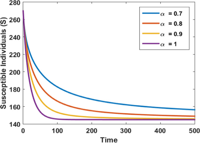
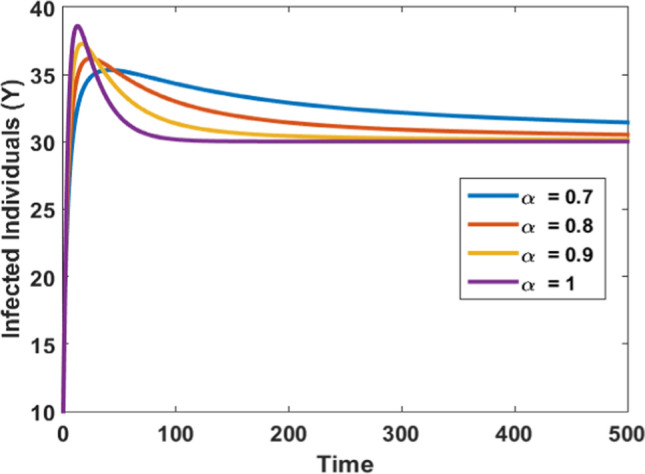
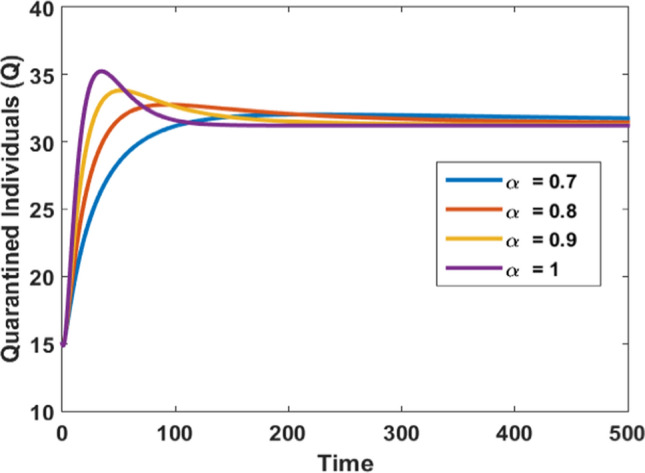
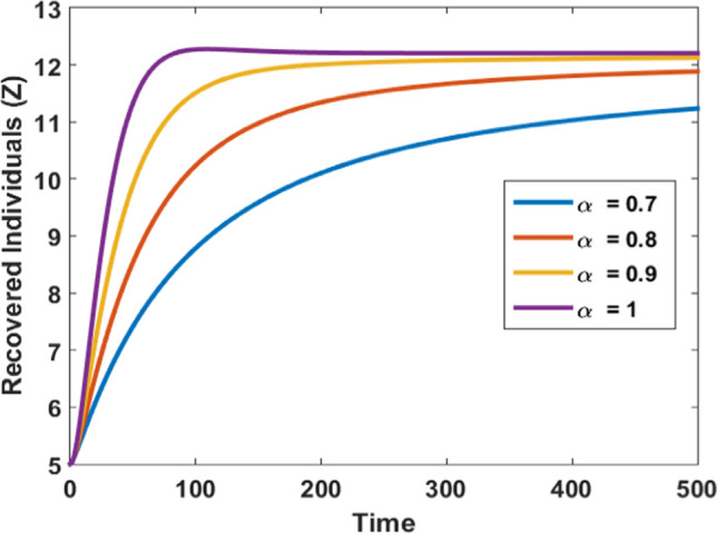
Figures 3, 4, 5, and 6 depict the impact of the fractional derivative of order $\alpha (\alpha =0.7,0.8,0.9,1)$ on the susceptible, infected, quarantined, and recovered subpopulations, respectively. On the ground of Theorem 5, the endemic equilibrium $E_2$ is stable for every value of fractional order $\alpha$ which is shown by these figures. Figures 3, 4, 5 and 6 also confirm that the disease is endemic as all the solution curves tend to the endemic equilibrium $E_2$. Further, from Figures 3, 4, 5 and 6, we observed that for $\alpha =1$, the system approaches the stationary state in a short duration. The stationary time is increased when we decrease the value of $\alpha$.

Fig. 3.

Impact of fraction order $\alpha$ on susceptible population

Fig. 4.

Impact of fraction order $\alpha$ on infected population

Fig. 5.

Impact of fraction order $\alpha$ on quarantine population

Fig. 6.

Impact of fraction order $\alpha$ on recovered population

Figure 3 depicts that for different values of $(\alpha (\alpha =0.7,0.8,0.9,1))$ as time passes, the number of susceptible individuals decreases, and finally the population reaches endemic equilibrium $E_2$ with time. It is noticed that as $\alpha$ approaches one, the system reaches the steady-state in a very short period.

Figure 4 shows the effect of fractional order derivative $\alpha$ on the infected individuals and it is observed that for the lower value of $\alpha$ steady time is increasing. As $\alpha$ approaches one the steady-state is achieved in a very short duration for infected populations which means infected populations will need more time to vanish when $\alpha$ decreases due to the presence of the memory effect.

Figure 5 depicts the effect of fractional order derivative $\alpha$ on the quarantined individuals and it is noticed that as the quarantine takes into account, for the lower value of $\alpha$ steady time is increased. As $\alpha$ approaches to the value one the steady-state is achieved in a very short time for the quarantined populations. It can be concluded from this figure that timely and effective quarantine can be proved a vital factor in the recovery of infectives and hence control the spread of infections.

Figure 6 shows that, if we decrease the fractional-order, the total number of recovered cases is decreased and it takes more time to approach to a steady-state. It is observed that as $\alpha$ increases then the number of recovered individuals also increases and as $\alpha$ reaches one steady state is achieved in a very short time.

Figure 7 depicts the infected individuals at various initial values of infected individuals ($Y\left(0\right)=5,10,15)$. It shows that when the number of infectives is low initially, infection occurs at a low level in comparison to high initial values of infected populations. Moreover, with any values of $Y(0)$, the infected population approaches the same steady-state as time passes.

Fig. 7.

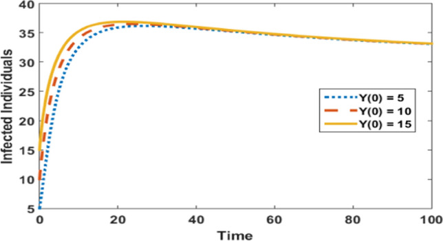
Impact of different initial values $Y(0)$ on the infected populations at $\alpha =0.8$

Figure 8 shows the impact of timely quarantine of individuals on the infected population. It is depicted that as the quarantine of individuals takes into account in the system then the infected population increases initially but later due to the timely quarantine of individuals, the infection reaches its peaks and then significantly decreases. Hence, timely quarantine of individuals is crucial to control the peak of infection during the epidemic outbreak.

Fig. 8.

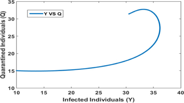
Quarantine population versus infected population at $\alpha =0.8$

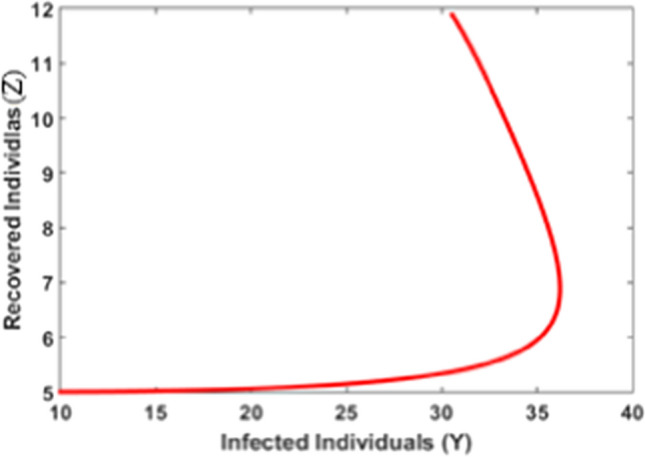
Figure 9 shows the impact of timely quarantine of individuals on the recovered population. It is obvious that as the quarantine takes place timely the recovery increases and reaches its steady state. In Fig. 10, it is observed that, initially, as the number of infected individuals increases recovered population is at a low level, and as time passes recovery increases with the increase of infected individuals and reaches its steady state.

Fig. 9.

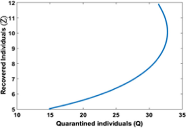
Quarantine population versus recovered population $\alpha =0.8$

Fig. 10.

Infected population versus recovered population $\alpha =0.8$

Figures 11 and 12 are portrayed to observe the impact of psychological effects on both susceptible and infected populations. As the value of the rate of psychological effects $\sigma$ increases, the number of susceptibles increases, and the peak of infected individuals start decreasing as shown in Fig. 11 and Fig. 12, respectively. Hence, the psychological effects can be used as an effective method for reducing the peak of infection in society during an outbreak.

Fig. 11.

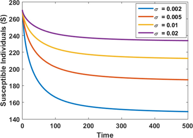
Impact of psychological effects $(\sigma )$ on the susceptible population at $\alpha =0.8$

Fig. 12.

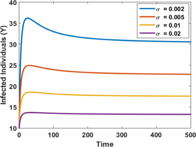
Impact of psychological effects $(\sigma )$ on infected individuals at $\alpha =0.8$

Discussion and Conclusion

This article aimed to propose and mathematically analyze a fractional-order epidemic model to understand the role of quarantine individuals along with a deep understanding of psychological effects on susceptible individuals in disease transmission dynamics during an outbreak. Therefore, a class of quarantined individuals is incorporated into the standard susceptible-infected- recovered-susceptible compartmental epidemic model with Monod-Haldane type incidence rate of infection. Monod-Haldane type incidence rate is a nonmonotonic incidence rate that considers the psychological effects on susceptibles during an epidemic. The Caputo derivative is considered for the population rate of each subpopulation. The Caputo derivative is a fractional-order derivative that considers the memory effects which can be seen for any emerging disease. Whenever a disease emerges in society, at the beginning of the disease, we always use the knowledge which we have collected from previously emerged diseases. This collected information is always helpful for controlling the transmission of newly emerging diseases and this is the memory effect in the fractional-order epidemic model that we cannot measure by the integer-order derivative-based epidemic model. The model analysis has shown that the proposed model is well-posed i.e. the solutions of the model are non-negative and bounded in a compact region; and the model has two equilibria, namely disease-free and endemic. Further, we computed the basic reproduction number $R_0$ by the Next-generation matrix method and investigated that the disease-free equilibrium is locally asymptotically stable when the basic reproduction number is less than the unity and unstable when it is greater than unity as stated in Theorem 3. The existence of a unique positive equilibrium is established and the local stability behavior of endemic equilibrium is analyzed. We investigated that EE is locally asymptotically stable when $R_0$ is greater than unity and follows any one condition of Lemma 4 as stated in Theorem 5. Furthermore, the global stability behaviors of both equilibria DFE and EE have been analyzed by the Lyapunov function method and it is shown that EE is globally asymptotically stable when $R_0>1$ and DFE is globally asymptotically stable when $R_0\le 1$ as stated in Theorems 6 and 7, respectively.

Numerical results are proposed in support of analytical results. Figure 2 is plotted in support of Theorem 3 which has shown that when $R_0<1$ then the disease-free equilibrium is locally asymptotically stable and when $R_0$ slightly increases from one then endemic equilibrium arrises. Figures 3, 4, 5, and 6 are plotted to show the impact of fractional order $\alpha$ on susceptible, infected, quarantine, and recovers subpopulations, respectively. These figures depict that as the value of fractional order $\alpha$ increases to one, each subpopulation takes less time to reach its steady state. We noticed that various values of $\alpha$ have no effect on the stability nature of the equilibrium points but affect only the time to reach the equilibrium state. These graphs support Theorem 5 which states that the EE is locally asymptotically stable when $R_0$ greater than one. It is also observed from the simulation that any initial population of infectives does not affect the steady-state of the infected population as shown in Fig. 7. Further, numerical simulations show that the timely quarantine of infected individuals helps us in reducing the new infection cases significantly, and also helps us in increment of recovered population. From graphs, it is observed that if we timely monitor the psychological effects and take the appropriate action to increase the value of the rate of psychological effects that helps to reduce the new infection significantly in society.

In conclusion, this study suggests that if health policymakers and professionals consider the memory effect, do the timely quarantine of infected individuals, and focus on the appropriate actions to increase the psychological effects on susceptibles then we can predict the disease more correctly, may reduce the impact of the epidemic, and this can also be helpful to reduce the period of the outbreak as well.

Appendix A

The matrix $V$ is $\left(\begin{array}{cccc}\gamma +\mu & -\delta & -\theta & 0\\ 0& d_2+\delta +\mu & -\omega & 0\\ 0& 0& d_1+\theta +\mu +\omega & 0\\ -\gamma & 0& \frac{A\beta }{\mu }& \mu \end{array}\right).$

Hence, the inverse of the matrix $V$ is given as:

$$V^{-1}=\left(\begin{array}{cccc}\frac{1}{\gamma +\mu }& \frac{\delta }{(\gamma +\mu )(d_2+\delta +\mu )}& \frac{\begin{array}{c}{d}_2\theta \mu +\delta \theta \mu \hfill \\ +\theta {\mu }^2+\delta \mu \omega \hfill \end{array}}{\mu (\gamma +\mu )(d_2+\delta +\mu )(d_1+\theta +\mu +\omega )}& 0\\ 0& \frac{1}{d_2+\delta +\mu }& \frac{\gamma \mu \omega +{\mu }^2\omega }{\mu (\gamma +\mu )(d_2+\delta +\mu )(d_1+\theta +\mu +\omega )}& 0\\ 0& 0& \frac{1}{d_1+\theta +\mu +\omega }& 0\\ \frac{d_2\gamma +\gamma \delta +\gamma \mu }{\mu (\gamma +\mu )(d_2+\delta +\mu )}& \frac{\gamma \delta }{\mu (\gamma +\mu )(d_2+\delta +\mu )}& \frac{\begin{array}{c}-\frac{A\beta \left(\gamma ,+,\mu \right)\left(d_2,+,\delta ,+,\mu \right)}{\mu }+\hfill \\ \gamma (d_2\theta +\delta \theta +\theta \mu +\delta \omega )\hfill \end{array}}{\mu (\gamma +\mu )(d_2+\delta +\mu )(d_1+\theta +\mu +\omega )}& \frac{1}{\mu }\end{array}\right)$$

Author contributions:

Both authors equally contributed to conceptualization, formal analysis, writing original draft, reviewing and editing.

Funding

The authors received no specific funding for this work.

Data availability

All relevant data are within the paper.

Code availability

Not Applicable.

Declarations

Conflict of interest

The authors declare that they have no conflicts of interest to disclose.

References

- Gumel AB, Mccluskey CC, Watmough J. An SVEIR model for assessing the potential impact of an imperfect anti-SARS vaccine. Math Biosci Eng. 2006;3:485–494. doi: 10.3934/mbe.2006.3.485. [DOI] [PubMed] [Google Scholar]
- Goel K, Kumar A, Nilam, A deterministic time-delayed SVIRS epidemic model with incidences and saturated treatment. J Eng Math. 2020;121:19–38. doi: 10.1007/s10665-020-10037-8. [DOI] [Google Scholar]
- Kumar A, Nilam, Stability of a delayed SIR epidemic model by introducing two explicit treatment classes along with nonlinear incidence rate and Holling type treatment. Comp Appl Math. 2019;38:130. doi: 10.1007/s40314-019-0866-9. [DOI] [Google Scholar]
- Kumar A, Nilam KR. A short study of an SIR model with Inclusion of an alert class two explicit nonlinear incidence rate and saturated treatment rate. SeMA J. 2019;76(3):505–519. doi: 10.1007/s40324-019-00189-8. [DOI] [Google Scholar]
- Kumar A. Stability of a fractional-order epidemic model with nonlinear incidences and treatments rates. Iran J Sci Technol Trans Sci. 2020;44:1505–1517. doi: 10.1007/s40995-020-00960-x. [DOI] [Google Scholar]
- Kermack, WO, Mckendrik, AGA (1927): A contribution to the mathematical theory of epidemics. Proc. R. Soc. A Math. Phys. Eng. Sci.; 115(772):700–721.
- Matignon D. Stability results for fractional differential equations with applications to control processing. IEEE-SMC Comput Eng Syst Appl. 1996;2:2963–2968. [Google Scholar]
- Kumar A, Nilam, Effects of nonmonotonic functional responses on a disease transmission model: modeling and simulation. Commun Math. Stat. 2021 doi: 10.1007/s40304-020-00217-4. [DOI] [PMC free article] [PubMed] [Google Scholar]
- Lu Z, Zhu Y. Comparison principles for fractional differential equations with the caputo derivatives. Adv Differ Equ. 2018;2018:237. doi: 10.1186/s13662-018-1691-y. [DOI] [Google Scholar]
- Haung G, Takeuchi Y, Ma W, Wei D. Global Stability for delay SIR and SEIR epidemic models with nonlinear incidence rate. Bull Math Biol. 2010;72:1192–1207. doi: 10.1007/s11538-009-9487-6. [DOI] [PubMed] [Google Scholar]
- Rostamy D, Mottaghi E. Stability analysis of a fractional order epidemics model with multiple equilibriums. Adv Differ Equ. 2016;2016:170. doi: 10.1186/s13662-016-0905-4. [DOI] [Google Scholar]
- Ahmed E, El-Sayed AMA, El-Saka HAA. On some Routh-Hurwitz conditions for fractional-order differential equations and their applications in Lorenz Rossler, Chua, Chen Systems. Phys Lett A. 2006;358(1):1–4. doi: 10.1016/j.physleta.2006.04.087. [DOI] [Google Scholar]
- Driessche PVD, Watmough J. Reproduction numbers and sub-threshold endemic equilibria for compartment models of disease transmission. Math Biosci. 2002;180:29–48. doi: 10.1016/S0025-5564(02)00108-6. [DOI] [PubMed] [Google Scholar]
- Goel K, Nilam, Stability behavior of a nonlinear mathematical epidemic transmission model with time delay. Nonlinear Dyn. 2019;98:1501–1518. doi: 10.1007/s11071-019-05276-z. [DOI] [Google Scholar]
- Wang X. A simple proof of Descartes’s rule of signs. Am Math Mon. 2004;111(6):525–526. doi: 10.1080/00029890.2004.11920108. [DOI] [Google Scholar]
- Alexander ME, Browman C, Moghadas SM, Summers R, Gumel AB, Sahai BM. A vaccination model for transmission dynamics of influenza. SIAM J Appl Dyn Syst. 2004;3(4):503–524. doi: 10.1137/030600370. [DOI] [Google Scholar]
- Podlubny I. Fractional differential equations. New York: Academic Press; 1999. [Google Scholar]
- Xu R, Ma Z. Stability of a delayed SIRS epidemic model with a nonlinear incidence rate. Chaos, Solutions and Fractals. 2009;41:2319–2325. doi: 10.1016/j.chaos.2008.09.007. [DOI] [Google Scholar]
- Ye X, Xu C. A fractional order epidemic model and simulation for avian influenza dynamics. Math Methods Appl Sci. 2019;42(14):4765–4779. doi: 10.1002/mma.5690. [DOI] [Google Scholar]
- Wang WD. Global behavior of an SEIRS epidemic model with time delays. Applied Mathematics Letter. 2002;15:423–428. doi: 10.1016/S0893-9659(01)00153-7. [DOI] [Google Scholar]
- Odibat ZM, Shawagfeh NT. Generalized Taylor’s formula. Appl Math Comput. 2007;186(1):286–293. [Google Scholar]
- Michael YL, Graef JR, Wang L, Karsai J. Global dynamics of a SEIR model with varying total population size. Math Biosci. 1999;160:191–213. doi: 10.1016/S0025-5564(99)00030-9. [DOI] [PubMed] [Google Scholar]
- La Salle JP. The stability of dynamical systems. Soc Ind Appl Math. 1976 doi: 10.1137/1.9781611970432. [DOI] [Google Scholar]
- Naik PA, Yavuz M, Qureshi S, Zu J, Townley S. Modeling and analysis of covid-19 epidemics with treatment in fractional derivatives using real data from Pakistan. Eur Phys J plus. 2020;135:795. doi: 10.1140/epjp/s13360-020-00819-5. [DOI] [PMC free article] [PubMed] [Google Scholar]
- Khan MA, Ullah S, Ullah S, Farhan M. Fractional order SEIR model with generalized incidence rate. AIMS Math. 2020;5(4):2843–2857. doi: 10.3934/math.2020182. [DOI] [Google Scholar]
- Goel K, Kumar A, Nilam, Nonlinear dynamics of a time- delayed epidemic model with two explicit aware classes, saturated incidences, and treatment. Nonlinear Dyn. 2020;101:1693–1715. doi: 10.1007/s11071-020-05762-9. [DOI] [PMC free article] [PubMed] [Google Scholar]
- Diethelm K, Ford NJ, Freed AD. A predictor-corrector approach for the numerical simulation of fractional differential equations. Nonlinear Dyn. 2002;29:3–22. doi: 10.1023/A:1016592219341. [DOI] [Google Scholar]
- MathsWorks (2012): Predictor–corrector PECE method for fractional differential equations, http:/www.mathworks.com/matlabcentral/fileexchange/32918.
- Camargo RF, Oliveira EC (2015): Cálculo fracionário. Livraria da Física, São Paulo.
- Saad KM, Baleanu D, Atangana A. New fractional derivatives applied to the Korteweg-de Vries and Korteweg-de Vries-Burger’s equations. Comput Appl Math. 2018;37(4):5203–5216. doi: 10.1007/s40314-018-0627-1. [DOI] [Google Scholar]
- Dubey P, Dubey B, Dubey US. An SIR model with nonlinear incidence rate and Holling type III treatment rate. Appl. Anal. Biol. Phys. Sci. Springer Proc. Math. Stat. 2016;186:63–81. doi: 10.1007/978-81-322-3640-5_4. [DOI] [Google Scholar]
- Liu WM, Levin SA, Iwasa Y. Influence of nonlinear incidence rates upon the behavior of SIRS epidemiological models. J Math Biol. 1986;23(2):187–204. doi: 10.1007/BF00276956. [DOI] [PubMed] [Google Scholar]
- Shi X, Zhou X, Song X. Analysis of a stage-structured predator-prey model with Crowley–Martin function. J Appl Math Comput. 2011;36(1–2):459–472. doi: 10.1007/s12190-010-0413-8. [DOI] [Google Scholar]
- Liu WM, Hethcote HW, Levin SA. Dynamical behavior of epidemiological models with nonlinear incidence rates. J Math Biol. 1987;25(4):359–380. doi: 10.1007/BF00277162. [DOI] [PubMed] [Google Scholar]
- Xiao D, Ruan S. Global analysis of an epidemic model with nonmonotone incidence rate. Math Biosci. 2007;208(2):419–429. doi: 10.1016/j.mbs.2006.09.025. [DOI] [PMC free article] [PubMed] [Google Scholar]
- Boukhouima A, Hattaf K, Lotfi EM, Mahrouf M, Torres DFM, Yousfi N. Lyapunov functions for fractional-order systems in biology: methods and applications. Chaos Solitons Fractals. 2020;140:110224. doi: 10.1016/j.chaos.2020.110224. [DOI] [Google Scholar]
- Erdem M, Safan M, Castillo-Chavez C. Mathematical analysis of an SIQR influenza model with imperfect quarantine. Bull Math Biol. 2017;79:1612–1636. doi: 10.1007/s11538-017-0301-6. [DOI] [PubMed] [Google Scholar]
- Hethcote H, Zhien M, Shengbing L. Effects of quarantine in six endemic models for infectious diseases. Math Bios. 2002;180(1–2):141–160. doi: 10.1016/S0025-5564(02)00111-6. [DOI] [PubMed] [Google Scholar]
- World Health Organization (2021): Considerations for quarantine of contacts of COVID-19 cases. https://www.who.int/publications/i/item/WHO-2019-nCoV-IHR-Quarantine-2021.1.
- Swati N. Fractional order SIR epidemic model with Beddington–De Angelis incidence and Holling type II treatment rate for Covid-19. J Appl Math Comput. 2022 doi: 10.1007/s12190-021-01658-y. [DOI] [PMC free article] [PubMed] [Google Scholar]
- Cui X, Xue D, Pan F. Dynamic analysis and optimal control for a fractional-order delayed SIR epidemic model with saturated treatment. Eur Phys J plus. 2022;137:586. doi: 10.1140/epjp/s13360-022-02810-8. [DOI] [PMC free article] [PubMed] [Google Scholar]
- Chatterjee AN, Basir FA, Ahmad B, Alsaedi A. A fractional-order compartmental model of vaccination for COVID-19 with the fear factor. Mathematics. 2022;10(9):1451. doi: 10.3390/math10091451. [DOI] [Google Scholar]
- Zhou X, Wang M. Dynamic analysis of a fractional-order SIRS model with time delay. Nonlinear Anal Model Control. 2022;27(2):368–384. [Google Scholar]
Associated Data
This section collects any data citations, data availability statements, or supplementary materials included in this article.
Data Availability Statement