Centered Partition Processes: Informative Priors for Clustering (with Discussion)

Abstract

There is a very rich literature proposing Bayesian approaches for clustering starting with a prior probability distribution on partitions. Most approaches assume exchangeability, leading to simple representations in terms of Exchangeable Partition Probability Functions (EPPF). Gibbs-type priors encompass a broad class of such cases, including Dirichlet and Pitman-Yor processes. Even though there have been some proposals to relax the exchangeability assumption, allowing covariate-dependence and partial exchangeability, limited consideration has been given on how to include concrete prior knowledge on the partition. For example, we are motivated by an epidemiological application, in which we wish to cluster birth defects into groups and we have prior knowledge of an initial clustering provided by experts. As a general approach for including such prior knowledge, we propose a Centered Partition (CP) process that modifies the EPPF to favor partitions close to an initial one. Some properties of the CP prior are described, a general algorithm for posterior computation is developed, and we illustrate the methodology through simulation examples and an application to the motivating epidemiology study of birth defects.

1. Introduction

Clustering is one of the canonical data analysis goals in statistics. There are two main strategies that have been used for clustering; namely, distance and model-based clustering. Distance-based methods leverage upon a distance metric between data points, and do not in general require a generative probability model of the data. Model-based methods rely on discrete mixture models, which model the data in different clusters as arising from kernels having different parameter values. The majority of the model-based literature uses maximum likelihood estimation, commonly relying on the EM algorithm. Bayesian approaches that aim to approximate a full posterior distribution on the clusters have advantages in terms of uncertainty quantification, while also having the ability to incorporate prior information.

Although this article is motivated by providing a broad new class of methods for improving clustering performance in practice, we were initially motivated by a particular application involving birth defects epidemiology. In this context, there are N = 26 different birth defects, which we can index using $i\in \left\{1,\dots ,N\right\}$, and for each defect i there is an highly variable number of observations. We are interested in clustering these birth defects into mechanistic groups, which may be useful, for example, in that birth defects in the same group may have similar coefficients in logistic regression analysis relating different exposures to risk of developing the defect. Investigators have provided us with an initial partition c₀ of the defects {1,…,N } into groups. It is appealing to combine this prior knowledge with information in the data from a grouped logistic regression to produce a posterior distribution on clusters, which characterizes uncertainty. The motivating question of this article is how to do this, with the resulting method ideally having broader impact to other types of centering of priors for clustering; for example, we may want to center the prior based on information on the number of clusters or cluster sizes.

With these goals in mind, we start by reviewing the relevant literature on clustering priors. Most of these methods assume exchangeability, which means that the prior probability of a partition c of {1,…,N } into clusters depends only on the number of clusters and the cluster sizes; the indices on the clusters play no role. Under the exchangeability assumption, one can define what is referred to in the literature as an Exchangeable Partition Probability Function (EPPF) (Pitman, 1995). This EPPF provides a prior distribution on the random partition c. One direction to obtain a specific form for the EPPF is to start with a nonparametric Bayesian discrete mixture model with a prior for the mixing measure P, and then marginalize over this prior to obtain an induced prior on partitions. Standard choices for P, such as the Dirichlet (Ferguson, 1973) and Pitman-Yor process (Pitman and Yor, 1997), lead to relatively simple analytic forms for the EPPF. There has been some recent literature studying extensions to broad classes of Gibbs-type processes (Gnedin and Pitman, 2006; De Blasi et al., 2015), mostly focused on improving flexibility while maintaining the ability to predict the number of new clusters in a future sample of data.

There is also a rich literature on relaxing exchangeability in various ways. Most of the emphasis has been on the case in which a vector of features x_i is available for index i, motivating feature-dependent random partitions models. Building on the stick-breaking representation of the DP (Sethuraman, 1994), MacEachern (1999, 2000) proposed a class of fixed weight dependent DP (DDP) priors. Applications of this DDP framework have been employed in ANOVA modeling (De Iorio et al., 2004), spatial data analysis (Gelfand et al., 2005), time series (Caron et al., 2006) and functional data analysis applications (Petrone et al., 2009; Scarpa and Dunson, 2009) among many others, with some theoretical properties highlighted in Barrientos et al. (2012).

However such fixed weight DDPs lack flexibility in feature-dependent clustering, as noted in MacEachern (2000). This has motivated alternative formulations which allow the mixing weights to change with the features, with some examples including the order-based dependent Dirichlet process (Griffin and Steel, 2006), kernel- (Dunson and Park, 2008), and probit- (Rodriguez and Dunson, 2011) stick breaking processes.

Alternative approaches build on random partition models (RPMs), working directly with the probability distribution p(c) on the partition c of indices {1,…,N} into clusters. Particular attention has been given to the class of product partition models (PPMs) (Barry and Hartigan, 1992; Hartigan, 1990) where p(c) can be factorized into a product of cluster-dependent functions, known as cohesion functions. A common strategy modifies the cohesion function to allow feature-dependence; refer, for examples, to Park and Dunson (2010), Müller et al. (2011), Blei and Frazier (2011), Dahl et al. (2017) and Smith and Allenby (2019).

Our focus is fundamentally different. In particular, we do not have features x_i on indices i but have access to an informed prior guess c₀ for the partition c; other than this information it is plausible to rely on exchangeable priors. To address this problem, we propose a general strategy to modify a baseline EPPF to include centering on c₀. In particular, our proposed Centered Partition (CP) process defines the partition prior as proportional to an EPPF multiplied by an exponential factor that depends on a distance function d(c, c₀), measuring how far c is from c₀. The proposed framework should be broadly useful in including extra information into EPPFs, which tend to face issues in lacking incorporation of real prior information from applications.

The paper is organized as follows. Section 2 introduces concepts and notation related to Bayesian nonparametric clustering. In Section 3 we illustrate the general CP process formulation and describe an approach to posterior computation relying on Markov chain Monte Carlo (MCMC). Section 4 proposes a general strategy for prior calibration building on a targeted Monte Carlo procedure. Simulation studies and application to the motivating birth defects epidemiology study are provided in Section 5, with technical details included in Paganin et al. (2020).

2. Clustering and Bayesian Models

This section introduces some concepts related to the representation of the clustering space from a combinatorial perspective, which will be useful to define the Centered Partition process, along with an introduction to Bayesian nonparametric clustering models.

2.1. Set Partitions

Let c be a generic clustering of indices [N ] = {1,…,N }. It can be either represented as a vector of indices {c₁,…, c_N}, with $c_i\in \left\{1,\dots ,K\right\}$ for i = 1,…,N and c_i = c_j when i and j belong to the same cluster, or as a collection of disjoint subsets (blocks) {B₁, B₂,…, B_K} where B_k contains all the indices of data points in the k-th cluster and K is the number of clusters in the sample of size N. From a mathematical perspective c = {B₁,…, B_K} is a combinatorial object known as set partition of [N ]. The collection of all possible set partitions of [N ], denoted with ${\text{Π}}_N$, is known as the partition lattice. We refer to Stanley (1997) and Davey and Priestley (2002) for an introduction to lattice theory, and to Meilă (2007) and Wade and Ghahramani (2018) for a review of the concepts from a more statistical perspective.

According to Knuth in Wilson and Watkins (2013), set partitions seem to have been studied first in Japan around A.D. 1500, due to a popular game in the upper class society known as genji-ko; five unknown incense sticks were burned and players were asked to identify which of the scents were the same, and which were different. Soon diagrams were developed to model all the 52 outcomes, which corresponds to all the possible set partitions of N = 5 elements. First results focused on enumerating the elements of the space. For example, for a fixed number of blocks K, the number of ways to assign N elements to K groups is described by the Stirling number of the second kind

$${𝒮}_{N,K}=\frac{1}{K!}\sum _{j=0}^K{\left(-1\right)}^j\left(\begin{array}{c}K\\ j\end{array}\right){\left(K-j\right)}^N,$$

while the Bell number ${ℬ}_N={\sum }_{K=1}^N{𝒮}_{N,K}$ describes the number of all possible set partitions of N elements.

Interest progressively shifted towards characterizing the structure of the space of partitions using the notion of partial order. Consider ${\text{Π}}_N$ endowed with the set containment relation ≤, meaning that for c = {B₁…, B_K}, ${\mathit{\text{c}}}^{\prime }=\left\{B_1^{\prime },\dots ,{B^{\prime }}_{K^{\prime }}\right\}$ belonging to ${\text{Π}}_N$, c ≤ c′ if for all $i=1,\dots ,K$, $B_i\subseteq B_j^{\prime }$ for some $j\in \left\{1,\dots ,K\prime \right\}$. Then the space $\left({\text{Π}}_N,\le \right)$ is a partially ordered set (poset), which satisfies the following properties:

1. Reflexivity: for every $\mathit{\text{c}}\in {\text{Π}}_N$, c ≤ c,

2. Antisymmetry: if c ≤ c′ and c′ ≤ c then c = c′,

3. Transitivity: if c ≤ c′ and c′ ≤ c′′, then c ≤ c′′.

Moreover, for any c, $\mathit{\text{c}}\prime \in {\text{Π}}_N$, it is said that c is covered (or refined) by c′ if c ≤ c′ and there is no c′′ such that c < c′′ < c′. Such a relation is indicated by $\mathit{\text{c}}\prec \mathit{\text{c}}\prime$. This covering relation allows one to represent the space of partitions using a Hasse diagram, in which the elements of ${\text{Π}}_N$ correspond to nodes in a graph and a line is drawn from c to c′ when $\mathit{\text{c}}\prec \mathit{\text{c}}\prime$; there is a connection from a partition c to another one when the second can be obtained by splitting or merging one of the blocks in c. See Figure 1 for an example of the Hasse diagram of Π₄. Conventionally, the partition with just one cluster is represented at the top of the diagram and denoted as 1, while the partition having every observation in its own cluster is at the bottom and indicated with 0.

Figure 1:

Hasse diagram for the lattice of set partitions of 4 elements. A line is drawn when two partitions have a covering relation. For example {1} {2, 3, 4} is connected with 3 partitions obtained by splitting the block {2, 3, 4} in every possible way, and with partition 1, obtained by merging the two clusters.

This representation of the set partitions space Π_N as a partially ordered set provides a useful framework to characterize its elements. As already mentioned, two partitions connected in the Hasse diagram can be obtained from one another by means of a single operation of split or merge; a sequence of connections is a path, linking the two extreme partitions 0 and 1. A path starting from 0 connects partitions with an increasing rank, which is related to the number of blocks through r(c) = N – |c |. Set partitions with the same rank may differ in terms of their configuration Λ(c), the sequence of block cardinalities {| B₁ |,…,|B_K|}, which corresponds to another combinatorial object known as an integer partition of N. In combinatorics, an integer partition is defined as the multiset of positive integers {λ₁ … λ_K}, listed in decreasing order by convention, such that ${\sum }_{i=1}^K{\lambda }_i=N$. Also the associated space of all possible integer partitions I_N is a partially ordered set, making the definition of configuration a poset mapping $\text{Λ}\left(\cdot \right):\mathit{\text{c}}\in {\text{Π}}_N\to \text{λ}\in I_N$.

Finally, the space Π_N is a lattice, based on the fact that every pair of elements has a greatest lower bound (g.l.b.) and a least upper bound (l.u.b.) indicated with the “meet” ∧ and the “join” ∨ operators, i.e. c ∧ c′ = g.l.b.(c, c′) and c ∨ c′ = l.u.b.(c, c′) and equality holds under a permutation of the cluster labels. An element $\mathit{\text{c}}\in {\text{Π}}_N$ is an upper bound for a subset $\mathit{\text{S}}\subseteq {\text{Π}}_N$ if s ≤ c for all $\text{s}\in \mathit{\text{S}}$, and it is the least upper bound for a subset $\mathit{\text{S}}\subseteq {\text{Π}}_N$ if c is an upper bound for S and c ≤ c′ for all upper bounds c′ of S. The lower bound and the greatest lower bound are defined similarly, and the definition applies also to the elements of the space I_N. Consider, as an example, c = {1}{2, 3, 4} and c′ = {3}{1, 2, 4}; their greatest lower bound is c ∧ c′ = {1}{3}{2, 4} while the lowest upper bound is c ∨ c′ = {1, 2, 3, 4}. Considering the Hasse diagram in Figure 1 the g.l.b. and l.u.b. are the two partitions which reach both c and c^′ through the shortest path, respectively from below and from above.

2.2. Bayesian Mixture Models

From a statistical perspective, set partitions are key elements in a Bayesian mixture model framework. The main underlying assumption is that observations y₁,…, y_N are independent conditional on the partition c, and their joint probability density can be expressed as

$$p\left(\text{y}\left|\mathit{\text{c}},\mathit{\text{θ}}\right.\right)=\underset{k=1}{\overset{K}{\mathbf{\text{Π}}}}\underset{i\in B_k}{\mathbf{\text{Π}}}p\left(y_i\left|{\theta }_k\right.\right)=\underset{k=1}{\overset{K}{\mathbf{\text{Π}}}}p\left({\text{y}}_k\left|{\theta }_k\right.\right),$$ (2.1)

with θ = (θ₁,…, θ_K) a vector of unknown parameters indexing the distribution of observations ${\text{y}}_k={\left\{y_i\right\}}_{i\in B_k}$ for each cluster k = 1,…,K. In a Bayesian formulation, a prior distribution is assigned to each possible partition c, leading to a posterior of the form

$$p\left(\mathit{\text{c}}\left|\text{y,}\mathit{\text{θ}}\right.\right)\propto p\left(\mathit{\text{c}}\right)\underset{k=1}{\overset{K}{\mathbf{\text{Π}}}}p\left({\text{y}}_k\left|{\theta }_k\right.\right).$$ (2.2)

Hence the set partition c is conceived as a random object and elicitation of its prior distribution is a critical issue in Bayesian modeling.

The first distribution one may use, in the absence of prior information, is the uniform distribution, which gives the same probability to every partition with $p\left(\mathit{\text{c}}\right)=1/{ℬ}_N$; however, even for small values of N the Bell number ${ℬ}_N$ is very large, making computation of the posterior intractable even for simple choices of the likelihood. This motivated the definition of alternative prior distributions based on different concepts of uniformity, with the Jensen and Liu (2008) prior favoring uniform placement of new observations in one of the existing clusters, and Casella et al. (2014) proposing a hierarchical uniform prior, which gives equal probability to set partitions having the same configuration.

Usual Bayesian nonparametric procedures build instead on discrete nonparametric priors, i.e. priors that have discrete realization almost surely. Dirichlet and Pitman-Yor processes are well known to have this property, as does the broader class of Gibbs-type priors. Any discrete random probability measure $\tilde{p}$ can induce an exchangeable random partition. Due to the discreteness of the process, $\tilde{p}$ induces a partition of the observations y₁,…, y_N which can be characterized via an Exchangeable Probability Partition Function. For both Dirichlet and Pitman-Yor processes, the EPPF is available in closed form as reported in Table 1 along with the case of the finite mixture model with κ components and a symmetric Dirichlet prior with parameters (γ/κ,…, γ/κ). Notice that λ_j = |B_j| is the cardinality of the clusters composing the partition, while notation (x)_r is for the rising factorial x(x + 1) ··· (x + r − 1).

Table 1:

Exchangeable Partition Probability Function for Dirichlet, Pitman-Yor processes and Symmetric Dirichlet distribution; λ_j = |B_j| is the cardinality of the clusters composing the partition, while ${\left(x\right)}_r=x\left(x+1\right)\cdots \left(x+r-1\right)$ denotes the rising factorial.

Random probability measure	Parameters	p(c) =
Dirichlet process	(α)	$\frac{{\alpha }^K}{{\left(\alpha \right)}_N}{\prod }_{j=1}^K\left({\lambda }_j-1\right)!$
Pitman-Yor process	(α, σ)	$\frac{{\prod }_{j=1}^{K-1}\left(\alpha +j\sigma \right)}{{\left(\alpha +1\right)}_{\left(N-1\right)}}{\prod }_{j=1}^K{\left(1-\sigma \right)}_{\left({\lambda }_j-1\right)}$
Symmetric Dirichlet	(κ, γ)	$\frac{\kappa !}{\left(\kappa -K\right)!}{\prod }_{j=1}^K\frac{\text{Γ}\left(\text{γ}/\kappa +{\lambda }_j\right)}{\text{Γ}\left(\text{γ}/\kappa \right)}$

There is a strong connection with the exchangeable random partitions induced by Gibbs-type priors and product partition models. A product partition model assumes that the prior probability for the partition c has the following form

$$p\left(\mathit{\text{c}}=\left\{B_1,\dots ,B_K\right\}\right)\propto \underset{j=1}{\overset{K}{\mathbf{\text{Π}}}}\rho \left(B_j\right),$$ (2.3)

with ρ(·) known as the cohesion function. The underlying assumption is that the prior distribution for the set partition c can be factorized as the product of functions that depend only on the blocks composing it. Such a definition, in conjunction with formulation (2.1) for the data likelihood, guarantees the property that the posterior distribution for c is still in the class of product partition models.

Distributions in Table 1 are all characterized by a cohesion function that depends on the blocks through their cardinality. Although the parameters can control the expected number of clusters, this assumption is too strict in many applied contexts in which prior information is available about the grouping. In particular, the same probability is given to partitions with the same configuration but having a totally different composition.

3. Centered Partition Processes

Our focus is on incorporating structured knowledge about clustering of the finite set of indices [N ] = {1,…,N } in the prior distribution within a Bayesian mixture model framework. We consider as a first source of information a given potential clustering, but our approach can also accommodate prior information on summary statistics such as the number of clusters and cluster sizes.

3.1. General Formulation

Assume that a potential clustering c₀ is given and we wish to include this information in the prior distribution. To address this problem, we propose a general strategy to modify a baseline EPPF to shrink towards c₀. In particular, our proposed CP process defines the prior on set partitions as proportional to a baseline EPPF multiplied by a penalization term of the type

$$p\left(\mathit{\text{c}}\left|{\mathit{\text{c}}}_0,\psi \right.\right)\propto p_0\left(\mathit{\text{c}}\right)e^{-\psi d\left(c,c_0\right)},$$ (3.1)

with ψ > 0 a penalization parameter, d(c, c₀) a suitable distance measuring how far c is from c₀ and p₀(c) indicates a baseline EPPF, that may depend on some parameters that are not of interest at the moment. For ψ → 0, $p\left(\mathit{\text{c}}\left|{\mathit{\text{c}}}_0,\psi \right.\right)$ corresponds to the baseline EPPF p₀(c), while for $\psi \to \infty$, $p\left(\mathit{\text{c}}={\mathit{\text{c}}}_0\left|{\mathit{\text{c}}}_0\right.,\psi \right)\to 1$.

Note that d(c, c₀) takes a finite number of discrete values Δ = {δ₀,…, δ_L}, with L depending on c₀ and on the distance d( ·, ·). We can define sets of partitions having the same fixed distance from c₀ as

$$s_l\left({\mathit{\text{c}}}_0\right)=\left\{\mathit{\text{c}}\in {\text{Π}}_N:d\left(\mathit{\text{c}},{\mathit{\text{c}}}_0\right)={\delta }_l\right\},l=0,1,\dots ,L.$$ (3.2)

Hence, for δ₀ = 0, s₀(c₀) denotes the set of partitions equal to the base one, meaning that they differ from c₀ only by a permutation of the cluster labels. Then s₁(c₀) denotes the set of partitions with minimum distance δ₁ from c₀, s₂(c₀) the set of partitions with the second minimum distance δ₂ from c₀ and so on. The introduced exponential term penalizes equally partitions in the same set s_l(c₀) for a given δ_l, but the resulting probabilities may differ depending on the chosen baseline EPPF.

3.2. Choices of Distance Function

The proposed CP process modifies a baseline EPPF to include a distance-based penalization term, which aims to shrink the prior distribution towards a prior partition guess. The choice of distance plays a key role in determining the behavior of the prior distribution. A variety of different distances and indices have been employed in clustering procedures and comparisons. We consider in this paper the Variation of Information (VI), obtained axiomatically in Meilă (2007) using information theory, and shown to nicely characterize neighborhoods of a given partition by Wade and Ghahramani (2018). The Variation of Information is based on the Shannon entropy H(·), and can be computed as

$$\begin{array}{l}\text{VI}\left(\mathit{\text{c}},\mathit{\text{c}}\prime \right)=-H\left(\mathit{\text{c}}\right)-H\left({\mathit{\text{c}}}_0\right)+2H\left(\mathit{\text{c}}\wedge {\mathit{\text{c}}}_0\right)\\ =\sum _{j=1}^K\frac{{\lambda }_j}{N}\log \left(\frac{{\lambda }_j}{N}\right)+\sum _{l=1}^{K\prime }\frac{\lambda \begin{array}{c}\prime \\ l\end{array}}{N}\log \left(\frac{\lambda \begin{array}{c}\prime \\ l\end{array}}{N}\right)-2\sum _{j=1}^K\sum _{l=1}^{K\prime }\frac{\lambda \begin{array}{c}\wedge \\ jl\end{array}}{N}\log \left(\frac{\lambda \begin{array}{c}\wedge \\ jl\end{array}}{N}\right),\end{array}$$

where log denotes log base 2, and $\lambda \begin{array}{c}\wedge \\ jl\end{array}$ the size of blocks of the intersection c ˄ c′ and hence the number of indices in block j under partition c and block l under c′. Notice that VI ranges from 0 to log₂(N ). Although normalized versions have been proposed (Vinh et al., 2010), some desirable properties are lost under normalization. We refer to Meilă (2007) and Wade and Ghahramani (2018) for additional properties and empirical evaluations.

An alternative definition of the VI can be derived from lattice theory, exploiting the concepts provided in Section 2.1. We refer to Monjardet (1981) for general theory about metrics on lattices and ordered sets, and Rossi (2015) for a more recent review focused on set partitions. In general, a distance between two different partitions $\mathit{\text{c}},\mathit{\text{c}}\prime \in {\text{Π}}_N$ can be defined by means of the Hasse diagram via the minimum weighted path, which corresponds to the shortest path length when edges are equally weighted. Instead, when edges depend on the entropy function through $w\left(\mathit{\text{c}},\mathit{\text{c}}\prime \right)=\left|H\left(\mathit{\text{c}}\right)-H\left(\mathit{\text{c}}\prime \right)\right|$, the minimum weighted path between two partitions is the Variation of Information. Notice that two partitions are connected when in a covering relation, then c ˄ c′ is either equal to c or c′ and V I(c, c′) = w(c, c′). The minimum weight w(c, c′) corresponds to 2/N which is attained when two singleton clusters are merged, or conversely, a cluster consisting of two points is split (see Meilă, 2007).

3.3. Effect of the Prior Penalization

We first consider the important special case in which the baseline EPPF is $p_0\left(\mathit{\text{c}}\right)=1/{ℬ}_N$ and the CP process reduces to $p\left(\mathit{\text{c}}\left|{\mathit{\text{c}}}_0,\psi \right.\right)\propto \exp \left\{-\psi d\left(\mathit{\text{c}},{\mathit{\text{c}}}_0\right)\right\}$ with equation (3.1) simplifying to

$$p\left(\mathit{\text{c}}\left|{\mathit{\text{c}}}_0,\psi \right.\right)=\frac{e^{-\psi {\delta }_l}}{{\sum }_{u=0}^L\left|s_u\left({\mathit{\text{c}}}_0\right)\right|e^{-\psi {\delta }_u}},\text{\hspace{0.17em}\hspace{0.17em}\hspace{0.17em}\hspace{0.17em}\hspace{0.17em}for\hspace{0.17em}\hspace{0.17em}\hspace{0.17em}}\mathit{\text{c}}\in s_l\left({\mathit{\text{c}}}_0\right),l=0,1,\dots ,L,$$ (3.3)

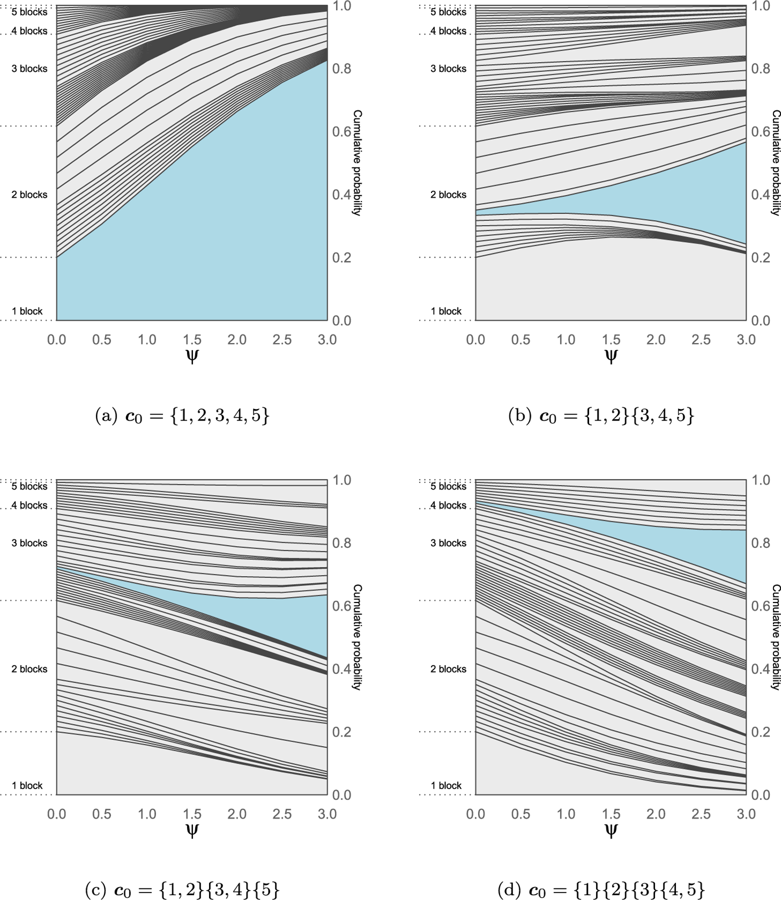
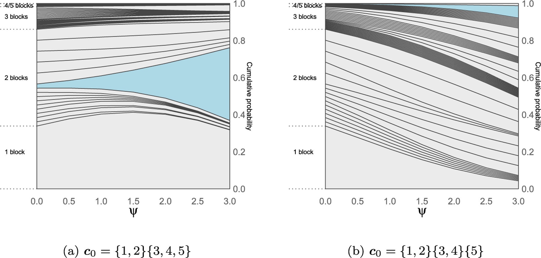
where | · | indicates the cardinality and s_l(c₀) is defined in (3.2). Considering N = 5, there are 52 possible set partitions; Figure 2 shows the prior probabilities assigned to partitions under the CP process for different values of $\psi \in \left(0,3\right)$ with ψ = 0 corresponding to the uniform prior. Notice that base partitions with the same configuration (e.g. for c₀ = {1, 2}{3, 4, 5} all the partitions with blocks sizes {3, 2}), will behave in the same way, with the same probabilities assigned to partitions different in composition. Non-zero values of ψ increase the prior probability of partitions c that are relatively close to the chosen c₀. However, the effect is not uniform but depends on the structure of both c and c₀.

Figure 2:

Prior probabilities of the 52 set partitions of N = 5 elements for the CP process with uniform base EPPF. In each graph the CP process is centered on a different partition c₀ highlighted in blue. The cumulative probabilities across different values of the penalization parameter ψ are joined to form the curves, while the probability of a given partition corresponds to the area between the curves.

For example, consider the inflation that occurs in the blue region as ψ increases from 0 to 3. When c₀ has 2 blocks (Figure 2a) versus 4 (Figure 2d) there is a bigger increase. This is because the space of set partitions Π_N is not “uniform”, since given a fixed configuration there is a heterogeneous number of partitions. Expressing λ = {λ₁,…, λ_K }as $\left(1^{f_1},2^{f_2},\dots ,N^{f_N}\right)$, with the notation indicating that there are f_i elements of λ equal to i, the number of set partitions with configuration λ is

$$\frac{N!}{{\text{Π}}_{j=1}^K{\lambda }_j!{\text{Π}}_{i=1}^N{f}_i!}.$$

For example, for {221} = 1¹2²3⁰4⁰5⁰, the number of corresponding set partitions is 15, while there are 10 set partitions of type {311} = 1²2⁰3¹4⁰5⁰.

While the uniform distribution gives the same probability to each partition in the space, the EPPF induced by Gibbs-type priors distinguishes between different configurations, but not among partitions with the same configuration. We focus on the Dirichlet process case, being the most popular process employed in applications. Under the DP, the induced EPPF $p_0\left(\mathit{\text{c}}\right)\propto {\alpha }^K{\text{Π}}_{j=1}^K\Gamma \left({\lambda }_j\right)$ is a function of the configuration Λ(c), which is one of {λ₁,…, λ_M } since the possible configurations are finite and correspond to the number of integer partitions. Letting $g\left(\text{Λ}\left(\mathit{\text{c}}\right)\right)={\alpha }^K{\text{Π}}_{j=1}^K\Gamma \left({\lambda }_j\right)$, the formulation in (3.1) can be written as

$$p\left(\mathit{\text{c}}\left|{\mathit{\text{c}}}_0,\psi \right.\right)=\frac{g\left({\text{λ}}_m\right)e^{-\psi {\delta }_l}}{{\sum }_{u=0}^L{\sum }_{\upsilon =1}^M{n}_{u\upsilon }g\left({\text{λ}}_{\upsilon }\right)e^{-\psi {\delta }_u}},\text{\hspace{0.17em}\hspace{0.17em}\hspace{0.17em}\hspace{0.17em}\hspace{0.17em}\hspace{0.17em}\hspace{0.17em}\hspace{0.17em}for\hspace{0.17em}\hspace{0.17em}\hspace{0.17em}}\mathit{\text{c}}\in s_{lm}\left({\mathit{\text{c}}}_0\right),$$ (3.4)

where $S_{lm}\left({\mathit{\text{c}}}_0\right)=\left\{\text{c}\in {\mathbf{\Pi }}_N:d\left(\mathit{\text{c}},{\mathit{\text{c}}}_0\right)={\delta }_l,\mathbf{\Lambda }\left(\mathit{\text{c}}\right)={\mathbf{\lambda }}_m\right\}$, the set of partitions with distance δ_l from c₀ and configuration λ_m for l = 0, 1,…,L and m = 1,…,M, with $n_{lm}$ indicating the cardinality. The factorization (3.4) applies for the family of Gibbs-type priors in general, with different expressions of g(Λ(c)).

In Figure 3 we consider the prior distribution induced by the CP process when the baseline EPPF p₀(c) comes from a Dirichlet process with concentration parameter α = 1, considering the same base partitions and values for ψ as in Figure 2. For the same values of the parameter ψ, the behavior of the CP process changes significantly due to the effect of the base prior. In particular, in the top left panel the CP process is centered on c₀ = {1, 2, 3, 4, 5}, the partition with only one cluster, which is a priori the most likely one for ψ = 0. In general, for small values of ψ the clustering process will most closely resemble that for a DP. As ψ increases, the DP prior probabilities decrease for partitions far from c₀ while increase for partitions close to c₀.

Figure 3:

Prior probabilities of the 52 set partitions of N = 5 elements for the CP process with Dirichlet process of α = 1 base EPPF. In each graph the CP process is centered on a different partition c₀ highlighted in blue. The cumulative probabilities across different values of the penalization parameter ψ are joined to form the curves, while the probability of a given partition corresponds to the area between the curves.

Finally we investigate in Figures 4–5 what happens to the prior partition probabilities of the CP process, when the baseline EPPF comes from a Pitman-Yor process. To allow comparison with the DP case, we choose the strength parameter α such that the a priori expected number of clusters matches the one under the DP case, log(5) ≈ 1.6. Choosing values of σ = (0.25, 0.75) leads to values of the strength parameter α equal to ( –0.004, –0.691) respectively. It can be noticed that for the smaller value of the discount parameter σ = 0.25 (Figure 4) the graphs resemble more the ones related to the DP process, while for σ = 0.75 the prior probability mass concentrates more on partitions with number of clusters close to the expected one.

Figure 4:

Prior probabilities of the 52 set partitions of N = 5 elements for the CP process with Pitman-Yor process base EPPF with σ = 0.25 and α ≈ −0.004, such that the expected number of clusters equal to log(5) ≈ 1.6. In each graph the CP process is centered on a different partition c₀ highlighted in blue. The cumulative probabilities across different values of the penalization parameter ψ are joined to form the curves, while the probability of a given partition corresponds to the area between the curves.

Figure 5:

Prior probabilities of the 52 set partitions of N = 5 elements for the CP process with Pitman-Yor process base EPPF with σ = 0.75 and α ≈ −0.691, such that the expected number of clusters equal to log(5) ≈ 1.6. In each graph the CP process is centered on a different partition c₀ highlighted in blue. The cumulative probabilities across different values of the penalization parameter ψ are joined to form the curves, while the probability of a given partition corresponds to the area between the curves.

3.4. Posterior Computation Under Gibbs-Type Priors

Certain MCMC algorithms for Bayesian nonparametric mixture models can be easily modified for posterior computation in CP process models. In particular, we adapt the so-called “marginal algorithms” developed for Dirichlet and Pitman-Yor processes. These methods are called marginal since the mixing measure P is integrated out of the model and the predictive distribution is used within a MCMC sampler. In the following, we recall Algorithm 2 in Neal (2000) and illustrate how it can be adapted to sample from the CP process posterior. We refer to Neal (2000) and references therein for an overview and discussion of methods for both conjugate and nonconjugate cases, and to Fall and Barat (2014) for adaptation to Pitman-Yor processes.

Let c be represented as an N -dimensional vector of indices {c₁,…, c_N } encoding cluster allocation and let θ_k be the set of parameters currently associated to cluster k. The prior predictive distribution for a single c_i conditionally on c⁻ⁱ = {c₁,…, c_i−1, c_i+1,…, c_N } is exploited to perform the Gibbs sampling step allocating observations to either a new cluster or one of the existing ones. Algorithm 2 in Neal (2000) updates each c_i sequentially for i = 1,…,N via a reseating procedure, according to the conditional posterior distribution

$$p\left(c_i=k|{\mathit{\text{c}}}^{-i},\mathit{\text{θ}},y_i\right)\propto \left\{\begin{array}{l}p\left(c_i=k|{\mathit{\text{c}}}^{-i}\right)p\left(y_i|{\theta }_k\right)k=1,\dots ,K^{-}\\ p\left(c_i=k|{\mathit{\text{c}}}^{-i}\right)\int p\left(y_i|\theta \right)d{G}_0\left(\theta \right)k=K^{-}+1,\end{array}\right.$$ (3.5)

with K⁻ the number of clusters after removing observation i. The conditional distribution p(c_i = k|c⁻ⁱ) is reported in Table 2 for different choices of the prior EPPF. Notice that, for the case of finite Dirichlet prior, the update consists only in the first line of equation (3.5), since the number of classes is fixed. For Dirichlet and Pitman-Yor processes, when observation i is associated to a new cluster, a new value for θ is sampled from its posterior distribution based on the base measure G₀ and the observation y_i. This approach is straightforward when we can compute the integral $\int p\left(y_i|\theta \right)d{G}_0\left(\theta \right)$, as will generally be the case when G₀ is a conjugate prior.

Table 2:

Conditional prior distribution for c_i given c⁻ⁱ under different choices of the EPPF. With K⁻ we denote the total number of clusters after removing the ith observation while ${\lambda }_k^{-i}$ is the corresponding size of cluster k.

Random probability measure	Parameters	$p\left(c_i=k|c^{-i}\right)\propto$
Dirichlet process	(α)	$\left\{\begin{array}{l}\frac{{\lambda }_k^{-i}}{\alpha +N-1}k=1,\dots ,K^{-}\\ \frac{\alpha }{\alpha +N-1}k=K^{-}+1\end{array}\right.$
Pitman-Yor process	(α, σ)	$\left\{\begin{array}{l}\frac{{\lambda }_k^{-i}-\sigma }{\alpha +N-1}k=1,\dots ,K^{-}\\ \frac{\alpha +\sigma K^{-}}{\alpha +N-1}k=K^{-}+1\end{array}\right.$
Symmetric Dirichlet	(κ, γ)	$\frac{{\lambda }_k^{-i}+\text{γ}/\kappa }{\alpha +N-1}k=1,\dots ,\kappa$

Considering the proposed CP process, the conditional distribution for c_i given c⁻ⁱ can still be computed, but it depends both on the base prior and the penalization term accounting for the distance between the base partition c₀ and the one obtained by assigning the observation i to either one of the existing classes $k\in \left\{1,\dots ,K^{-}\right\}$ or a new one. Hence, the step in equation (3.5) can be easily adapted by substituting the conditional distribution for p(c_i = k|c⁻ⁱ) with

$$p\left(c_i=k|{\mathit{\text{c}}}^{-i},{\mathit{\text{c}}}_0,\psi \right)\propto p_0\left(c_i=k|{\mathit{\text{c}}}^{-i}\right)\exp \left\{-\psi d\left(\mathit{\text{c}},{\mathit{\text{c}}}_0\right)\right\}k=1,\dots K^{-},K^{-}+1,$$

with $\mathit{\text{c}}=\left\{{\mathit{\text{c}}}^{-i}\cup \left\{c_i=k\right\}\right\}$ the current state of the clustering and p₀(c_i = k|c⁻ⁱ) one of the conditional distributions in Table 2. Additional steps on the implementation using the variation of information as a distance are given in the Supplementary Material (Algorithm 2).

Extension to the non-conjugate context can be similarly handled exploiting Algorithm 8 in Neal (2000) based on auxiliary parameters, which avoids the computation of the integral $\int p\left(y_i|\theta \right)d{G}_0\left(\theta \right)$. The only difference is that, when c_i is updated, m temporary auxiliary variables are introduced to represent possible values of components parameters that are not associated with any other observations. Such variables are simply sampled from the base measure G₀, with the probabilities of a new cluster in Table 2 changing into (α/m)/(α + N − 1) for the Dirichlet process and to [(α + σK⁻)/m]/(α + N− 1) for the Pitman-Yor process, for k = K⁻ + 1,…,K⁻ + m.

4. Prior Calibration

As the number of observations N increases, the number of partitions explodes, and higher values of ψ are needed to place non-negligible prior probability in small to moderate neighborhoods around c₀. The prior concentration around c₀ depends on three main factors: i) N through ℬ_N, i.e. the cardinality of the space of set partitions, ii) the baseline EPPF p₀(c) and iii) where c₀ is located in the space. We hence propose a general method to evaluate the prior behavior under different settings, while suggesting how to choose the parameter ψ.

One may evaluate the prior distribution for different values of ψ and check its behavior using graphs such as those in Section 3.3, but they become difficult to interpret as the space of partitions grows. We propose to evaluate the probability distribution of the distances δ = d(c, c₀) from the known partition c₀. The probability assigned to different distances by the prior is

$$p\left(\delta ={\delta }_l\right)=\sum _{\mathit{\text{c}}\in {\text{Π}}_N}p\left(\mathit{\text{c}}\right)ℐ\left\{\left.d\left(\mathit{\text{c}},{\mathit{\text{c}}}_0\right)={\delta }_l\right)\right\}=\sum _{\mathit{\text{c}}\in s_l\left({\mathit{\text{c}}}_0\right)}p\left(\mathit{\text{c}}\right)l=0,\dots ,L,$$

with $ℐ\left(\cdot \right)$ the indicator function and s_l(c₀) denoting the set of partitions distance δ_l from c₀, as defined in (3.2). Considering the uniform distribution on set partitions, then p(δ = δ_l) = |s_l(c₀) |/ℬ_N, the proportion of partitions distance δ_l from c₀. Under the general definition of the CP process, the resulting distribution becomes

$$p\left(\delta ={\delta }_l\right)=\sum _{\mathit{\text{c}}\in s_l\left({\mathit{\text{c}}}_0\right)}\frac{p_0\left(\mathit{\text{c}}\right)e^{-\psi {\delta }_l}}{{\sum }_{u=0}^L{\sum }_{{\mathit{\text{c}}}^{\ast }\in s_u\left({\mathit{\text{c}}}_0\right)}{p}_0\left({\mathit{\text{c}}}^{\ast }\right)e^{-\psi {\delta }_u}}l=0,\dots ,L,$$ (4.1)

with the case of Gibbs-type EPPF corresponding to

$$p\left(\delta ={\delta }_l\right)=\frac{{\sum }_{m=1}^M{n}_{lm}g\left({\mathbf{\lambda }}_m\right)e^{-\psi {\delta }_l}}{{\sum }_{u=0}^L{\sum }_{v=1}^M{n}_{uv}g\left({\mathbf{\lambda }}_v\right)e^{-\psi {\delta }_u}},l=0,\dots ,L.$$ (4.2)

Notice that the uniform EPPF case is recovered when g(λ_m) = 1 for m = 1,…,M, so that ${\sum }_{m=1}^M{n}_{lm}=n_l$. Hence the probability in (4.1) simplifies to

$$p\left(\delta ={\delta }_l\right)=\frac{n_l{e}^{-\psi {\delta }_l}}{{\sum }_{u=0}^L{n}_u{e}^{-\psi {\delta }_u}}l=0,\dots ,L.$$ (4.3)

In general, since distances are naturally ordered, the corresponding cumulative distribution function can be simply defined as $F\left(\delta \right)={\sum }_{{\delta }_l\le \delta }p\left({\delta }_l\right)$ for $\delta \in \left\{{\delta }_0,\dots ,{\delta }_L\right\}$ and used to assess how much mass is placed in different size neighborhoods around c₀ under different values of ψ. Hence we can choose ψ to place a specified probability q (e.g. q = 0.9) on partitions within a specified distance δ^∗ from c₀. This would correspond to calibrating ψ so that F (δ^∗) ≈ q, with F (δ^∗) ≥ q. In other words, partitions generated from the prior would have at least probability q of being within distance δ^∗ from c₀.

The main problem is in computing the probabilities in equations (4.2)–(4.3), which depend on all the set partitions in the space. In fact, one needs to count all the partitions having distance δ_l for l = 0,…,L when the base EPPF is uniform, while taking account of configurations in the case of the Gibbs-type priors. Even if there are quite efficient algorithms to list all the possible set partitions of N (see Knuth, 2005; Nijenhuis and Wilf, 2014), it becomes computationally infeasible due to the extremely rapid growth of the space; for example from N = 12 to 13, the number of set partitions grows from ℬ₁₂ = 4, 213, 597 to ℬ₁₃ = 27, 644, 437.

Given that our motivating application involves a relatively small number of birth defects, we propose to directly approximate the prior probabilities assigned to different distances from c₀. We focus on obtaining estimates of distance values and related counts, which are the sufficient quantities to compute (4.2)–(4.3) under different values of ψ. We propose a strategy based on a targeted Monte Carlo procedure which augments uniform sampling on the space of set partitions with a deterministic local search using the Hasse diagram to compute counts for small values of the distance. Although the procedure is generalizable to higher dimensions, the computational burden grows significantly with larger numbers of objects to cluster. Alternative computational directions are considered further in the Discussion.

4.1. Deterministic Local Search

Poset theory provides a nice representation of the space of set partitions by means of the Hasse diagram illustrated in Section 2.1, along with suitable definition of metrics. A known partition c₀ can be characterized in terms of number of blocks K₀ and configuration Λ(c₀). These elements allow one to locate c₀ in the Hasse diagram, and hence explore connected partitions by means of split and merge operations on the clusters in c₀.

As an illustrative example, consider the Hasse diagram of Π₄ in Figure 6 and c₀ = {1}{2, 3, 4}, having 2 clusters and configuration Λ(c₀) = {31}. Let ${𝒩}_1\left({\mathit{\text{c}}}_0\right)$ denote the sets of partitions directly connected with c₀, i.e. partitions covering c₀ and those covered by c₀. In general, a partition c₀ with K₀ clusters is covered by $\left(\begin{array}{c}{K}_0\\ 2\end{array}\right)$ partitions and covers ${\sum }_{j=1}^{K_0}{2}^{{\lambda }_j-1}-1$. In the example, ${𝒩}_1\left({\mathit{\text{c}}}_0\right)$ contains {1, 2, 3, 4} obtained from c₀ with a merge operation on the two clusters, and all the partitions obtained by splitting the cluster {2, 3, 4} in any possible way. The idea underlying the proposed local search, consists in exploiting the Hasse diagram representation to find all the partitions in increasing distance neighborhoods of c₀. One can list partitions at T connections from c₀ starting from ${𝒩}_1\left({\mathit{\text{c}}}_0\right)$ by recursively applying split and merge operations on the set of partitions explored at each step. Potentially, with enough operations one can reach all the set partitions, since the space is finite with lower and upper bounds.

Figure 6:

Illustration of results from the local search algorithm based on the Hasse diagram of Π₄ starting from c₀ = {1}{2,3,4}. Partitions are colored according the exploration order following a dark-light gradient. Notice that after 3 iterations the space is entirely explored.

In practice, the space is too huge to be explored entirely, and a truncation is needed. From the example in Figure 6, ${𝒩}_1\left({\mathit{\text{c}}}_0\right)$ contains 3 partitions with distance 0.69 from c₀ and one with distance 1.19. Although ${𝒩}_2\left({\mathit{\text{c}}}_0\right)$ may contain partitions closer to c₀ than this last, the definition of distance in Section 3.2 guarantees that there are no other partitions with distance from c₀ less than 0.69. Since the VI is the minimum weighted path between two partitions, all the partitions reached at the second exploration step add a nonzero weight to distance computation. This consideration extends to an arbitrary number of explorations T, with ${\delta }_{L\ast }=\min {\left\{d\left({\mathit{\text{c}}}^{\ast },{\mathit{\text{c}}}_0\right)\right\}}_{{\mathit{\text{c}}}^{\ast }\in {𝒩}_T\left({\mathit{\text{c}}}_0\right)}$ being the upper bound on the distance value. By discarding all partitions with distance greater that δ_L∗, one can compute exactly the counts in equations (4.2)–(4.3) related to distances δ₀,…, δ_L∗. Notice that 2/N is the minimum distance between two different partitions, and 2T /N is a general lower bound on the distances from c₀ that can be reached in T iterations.

4.2. Monte Carlo Approximation

We pair the local exploration with a Monte Carlo procedure to estimate the counts and distances greater that δ_L∗, in order to obtain a more refined representation of the prior distance probabilities. Sampling uniformly from the space of partitions is not in general a trivial problem, but a nice strategy has been proposed in Stam (1983), in which the probability of a partition with K clusters is used to sample partitions via an urn model. Derivation of the algorithm starts from the Dobiński formula (Dobiński, 1877) for the Bell numbers

$${ℬ}_N=e^{-1}\sum _{k=1}^{\infty }\frac{k^N}{k!},$$ (4.4)

which from a probabilistic perspective corresponds to the N -th moment of the Poisson distribution with expected value equal to 1. Then a probability distribution for the number of clusters $K\in \left\{1,2,3,\dots \right\}$ of a set partition can be defined as

$$P\left(K=k\right)=e^{-1}\frac{k^N}{{ℬ}_{N}k!},$$ (4.5)

which is a well defined law thanks to (4.4). To simulate a uniform law over Π_N, Stam (1983)’s algorithm first generates the number of clusters K according to (4.5) and, conditionally on the sampled value, it allocates observations to the clusters according a discrete uniform distribution over {1,…,K}. We refer to Stam (1983) and Pitman (1997) (Proposition 2, Corollary 3) for derivations and proof of the validity of the algorithm.

We adapt the uniform sampling to account for the values already computed by rejecting all the partitions with distance less that δ_L∗, restricting the space to $\left\{{\text{Π}}_N\backslash {\left\{{𝒩}_t\left({\mathit{\text{c}}}_0\right)\right\}}_{t=0}^T\right\}$. In practice, few samples are discarded since the probability to sample one such partition corresponds to $\left|{\left\{{𝒩}_t\left({\mathit{\text{c}}}_0\right)\right\}}_{t=0}^T\right|/{ℬ}_N$, which is negligible for small values of exploration steps T that are generally used in the local search. A sample of partitions c⁽¹⁾,…, c^(R), can be used to provide an estimate of the counts. Let R^∗ de-note the number of accepted partitions and ${ℬ}^{\ast }={ℬ}_N-\left|{\left\{{𝒩}_t\left({\mathit{\text{c}}}_0\right)\right\}}_{t=0}^T\right|$ be the number of partitions in the restricted space. Conditionally on the observed values of distances in the sample, ${\widehat{\delta }}_{\left(L*+1\right)},\dots ,{\widehat{\delta }}_{L^{\prime }}$, an estimate of the number of partitions with distance ${\widehat{\delta }}_l$ to use in the uniform EPPF case is

$${\widehat{n}}_l={ℬ}^{*}\frac{1}{R^{*}}\sum _{r=1}^{R^{*}}ℐ\left\{d\left({\mathit{\text{c}}}^{\left(r\right)},{\mathit{\text{c}}}_0\right)={\widehat{\delta }}_l\right\},$$ (4.6)

obtained by multiplying the proportions of partitions in the sample by the total known number of partitions. For the Gibbs-type EPPF case one needs also to account for the configurations λ₁,…, λ_M in a given orbital of the distance; hence, the estimates are

$${\widehat{n}}_{lm}={ℬ}^{*}\frac{1}{R^{*}}\sum _{r=1}^{R^{*}}ℐ\left\{d\left({\mathit{\text{c}}}^{\left(r\right)},{\mathit{\text{c}}}_0\right)={\widehat{\delta }}_l\right\}ℐ\left\{\mathbf{\Lambda }\left({\mathit{\text{c}}}^{\left(r\right)}\right)={\mathbf{\lambda }}_m\right\}.$$ (4.7)

Pairing these estimates with the counts obtained via the local search, one can evaluate the distributions in equations (4.2)–(4.3) for different values of ψ. The entire procedure is summarized in Algorithm 1 of the Supplementary Material. Although it requires a considerable number of steps, the procedure can be performed one single time providing information for different choices of ψ and EPPFs. Moreover the local search can be implemented in parallel to reduce computational costs.

We consider an example for N = 12 and c₀ with configuration {3, 3, 3, 3}. Figure 7 shows the resulting cumulative probability estimates of the CP process under uniform and DP(α = 1) base distributions, estimated with T = 4 iterations of the local search and 20,000 samples. Dots represent values of the cumulative probabilities, with different colors in correspondence to different values of the parameter ψ. Using these estimates one can assess how much probability is placed in different distance neighborhoods of c₀; tables in Figure 7 show the distance values defining neighborhoods around c₀ with 90% prior probability. If one wishes to place such probability mass on partitions within distance 1 from c₀, a value of ψ around 10 and 15 is needed, respectively, under uniform and DP base EPPF prior.

Figure 7:

Estimate of the cumulative prior probabilities assigned to different distances from c₀ for N = 12 and c₀ with configuration {3, 3, 3, 3}, under the CP process with uniform prior on the left and Dirichlet Process on the right. Black dots correspond to the base prior with no penalization, while dots from bottom-to-top correspond to increasing values of $\psi \in \left\{5,10,15,20\right\}$. Tables report the minimum distance values such that F (δ) ≥ 0.9.

5. The National Birth Defects Prevention Study

The National Birth Defects Prevention Study (NBDPS) is a multi-state population-based, case-control study of birth defects in the United States (Yoon et al., 2001). Infants were identified using birth defects surveillance systems in recruitment areas within ten US states (Arkansas, California, Georgia, Iowa, Massachusetts, New Jersey, New York, North Carolina, Texas, and Utah), which cover roughly 10% of US births. Diagnostic case information was obtained from medical records and verified by a standardized clinician review specific to the study (Rasmussen et al., 2003). Participants in the study included mothers with expected dates of delivery from 1997–2009. Controls were identified from birth certificates or hospital records and were live-born infants without any known birth defects. Each state site attempted to recruit 300 cases and 100 (unmatched) controls annually. A telephone interview was conducted with case and control mothers to solicit a wide range of demographic, lifestyle, medical, nutrition, occupational and environmental exposure history information.

Because birth defects are highly heterogeneous, a relatively large number of defects of unknown etiology are included in the NBDPS. We are particularly interested in congenital heart defects (CHD), the most common type of birth defect and the leading cause of infant death due to birth defects. Because some of these defects are relatively rare, in many cases we lack precision for investigating associations between potential risk factors and individual birth defects. For this reason, researchers typically lump embryologically distinct and potentially etiologically heterogeneous defects in order to increase power (e.g., grouping all heart defects together), even knowing the underlying mechanisms may differ substantially. In fact, how best to group defects is subject to uncertainty, despite a variety of proposed groupings available in the literature (Lin et al., 1999).

In this particular application, we consider 26 individual heart defects, which have been previously grouped into 6 categories by investigators (Botto et al., 2007). The prior grouping is shown in Table 3, along with basic summary statistics of the distribution of defects in the analyzed data. We are interested in evaluating the association between heart defects and about 90 potential risk factors related to mothers’ health status, pregnancy experience, lifestyle and family history. We considered a subset of data from NBDPS, excluding observations with missing covariates, obtaining a dataset with 8,125 controls, while all heart defects together comprise 4,947 cases.

Table 3:

Summary statistics of the distribution of congenital heart defects among cases. Defects are divided according the grouping provided from investigators.

Congenital Heart Defect	Abbreviation	Frequency	Percentage of cases
Septal
Atrial septal defect	ASD	765	0.15
Perimembranous ventricular septal defect	VSDPM	552	0.11
Atrial septal defect, type not specified	ASDNOS	225	0.04
Muscular ventricular septal defect	VSDMUSC	68	0.02
Ventricular septal defect, otherwise specified	VSDOS	12	0.00
Ventricular septal defect, type not specified	VSDNOS	8	0.00
Atrial septal defect, otherwise specified	ASDOS	4	0.00
Conotruncal
Tetralogy of Fallot	FALLOT	639	0.12
D-transposition of the great arteries	DTGA	406	0.08
Truncus arteriosus	COMMONTRUNCUS	61	0.01
Double outlet right ventricle	DORVTGA	35	0.01
Ventricular septal defect reported as conoventricular	VSDCONOV	32	0.01
D-transposition of the great arteries, other type	DORVOTHER	22	0.00
Interrupted aortic arch type B	IAATYPEB	13	0.00
Interrupted aortic arch, not otherwise specified	IAANOS	5	0.00
Left ventricular outflow
Hypoplastic left heart syndrome	HLHS	389	0.08
Coarctation of the aorta	COARCT	358	0.07
Aortic stenosis	AORTICSTENOSIS	224	0.04
Interrupted aortic arch type A	IAATYPEA	12	0.00
Right ventricular outflow
Pulmonary valve stenosis	PVS	678	0.13
Pulmonary atresia	PULMATRESIA	100	0.02
Ebstein anomaly	EBSTEIN	66	0.01
Tricuspid atresia	TRIATRESIA	46	0.01
Anomalous pulmonary venous return
Total anomalous pulmonary venous return	TAPVR	163	0.03
Partial anomalous pulmonary venous return	PAPVR	21	0.01
Atrioventricular septal defect
Atrioventricular septal defect	AVSD	112	0.02

5.1. Modeling Birth Defects

Standard approaches assessing the impact of exposure factors on the risk to develop a birth defect often rely on logistic regression analysis. Let i = 1,…,N index birth defects, while j = 1,…, n_i indicates observations related to birth defect i, with y_ij = 1 if observation j has birth defect i and y_ij = 0 if observation j is a control, i.e. does not have any birth defect. Let X_i denote the data matrix associated to defect i, with each row ${\mathbf{x}}_{ij}^T=\left(x_{ij1},\dots x_{ijp}\right)$ being the vector of the observed values of p categorical variables for the jth observation. At first one may consider N separate logistic regressions of the type

$$\log \left(\frac{\text{pr}\left(y_{ij}=1|{\mathbf{x}}_{ij}\right)}{\text{pr}\left(y_{ij}=0|{\mathbf{x}}_{ij}\right)}\right)=\log \text{it}\left({\text{π}}_{ij}\right)={\alpha }_i+{\mathbf{x}}_{ij}^T{\text{β}}_i,$$ (5.1)

with α_i denoting the defect-specific intercept, and βi the p × 1 vector of regression coefficients. However, Table 3 highlights the heterogeneity of heart defect prevalences, with some of them being so few as to preclude separate analyses.

A first step in introducing uncertainty about clustering of the defects may rely on a standard Bayesian nonparametric approach, placing a Dirichlet process prior on the distribution of regression coefficient vector βi in order to borrow information across multiple defects while letting the data inform on the number and composition of the clusters. A similar approach has been previously proposed in MacLehose and Dunson (2010), with the aim being to shrink the coefficient estimates towards multiple unknown means. In our setting, an informed guess on the group structure is available through c₀, reported in Table 3.

We consider a simple approach building on the Bayesian version of the model in (5.1), and allowing the exposure coefficients βi for i = 1,…,N to be shared across regressions, while accounting for c₀. The model written in a hierarchical form is

$$\begin{array}{cc}{y}_{ij}\sim Ber\left({\pi }_{ij}\right)& \log \text{it}\left({\pi }_{ij}\right)={\alpha }_i+{\mathbf{x}}_{ij}^T{\text{β}}_{ci},j=1,\dots n_i,\\ {\alpha }_i~𝒩\left(a_0,{\tau }_0^{-1}\right)& {\text{β}}_{c_i}|\text{c~}{𝒩}_p\left(\mathbf{b},\mathbf{Q}\right)i=1,\dots N,\\ p\left(\mathit{\text{c}}\right)~CP\left({\mathit{\text{c}}}_0,\psi ,p_0\left(\mathit{\text{c}}\right)\right)& p_0\left(\mathit{\text{c}}\right){\propto }^K\prod _{k=1}^K\left({\lambda }_k-1\right)!\end{array}$$ (5.2)

where CP (c₀, ψ, p₀(c)) indicates the Centered Partition process, with base partition c₀, tuning parameter ψ and baseline EPPF p₀(c). We specify the baseline EPPF so that when ψ = 0 the prior distribution reduces to a Dirichlet Process with concentration parameter α. Instead, for ψ →∞ the model corresponds to K separate logistic regressions, one for each group composing c₀. The model estimation can be performed by leveraging a Pòlya-Gamma data-augmentation strategy for Bayesian logistic regression (Polson et al., 2013), combined with the procedure illustrated in Section 3.4 for the clustering update step. The Gibbs sampler is detailed in the Supplementary Material (Algorithm 3), while code is available at https://github.com/salleuska/CPLogit.

5.2. Simulation Study

We conduct a simulation study to evaluate the performance of our approach in accurately estimating the impact of the covariates across regressions with common effects, under different prior guesses. In this section we choose a scenario mimicking the structure of our application. An additional simulation study under a continuous setting can be found in the Supplementary Material.

In simulating data we take a number of defects N = 12 equally partitioned in 4 groups and consider p = 10 dichotomous explanatory variables, under the assumption that defects in the same group have the same covariates effects. We take a different number of observations across defects, with {n₁, n₂, n₃} = {100, 600, 200}, {n₄, n₅, n₆} = {300, 100, 100}, {n₇, n₈, n₉} = {500, 100, 200}, {n₁₀, n₁₁, n₁₂} = {200, 200, 200}. For each defect i with i = 1,…, 12 we generate a data matrix X_i by sampling each of the variables from a Bernoulli distribution with probability of success equal to 0.5. We set most of coefficients β_i1,…, β_i10 to 0, while defining a challenging scenario with small to moderate changes across different groups. In particular we fix {β₁, β₂, β₃, β₄} = {0.7, −1.2, 0.5, 0.5} for group 1, {β₄, β₅, β₆} = {0.7, −0.7, 0.7} for group 2, {β₉, β₁₀} = {0.7, −1.2} for group 3 and {β₁, β₂, β₉, β₁₀} = {0.7, −0.7, 0.7, −0.7} for group 4. Finally, response variables y_i for i = 1,…, 12 are drawn from a Bernoulli distribution with probability of success $p_i=\log \text{it}\left({\mathbf{X}}_i^T{\beta }_i\right)$.

We compare coefficients and partition estimates from a grouped logistic regression using a DP prior with α = 1 and using a CP prior with DP base EPPF with α = 1. In evaluating the CP prior performances, we consider both the true known partition and a wrong guess. Posterior estimates are obtained using the Gibbs sampler described in the Supplementary Material. We consider a multivariate normal distribution with zero mean vector and covariance matrix Q = diag_p(2) as base measure for the DP, while we assume the defect-specific intercepts α_i ∼ N (0, 2) for i = 1,…, 12. We run the algorithm for 5,000 iterations discarding the first 1,000 as burn-in, with inspection of trace-plots suggesting convergence of the parameters.

In evaluating the resulting estimates under different settings, we take as baseline values for coefficients the maximum likelihood estimates obtained under the true grouping. Figure 8 shows the posterior similarity matrices obtained under the Dirichlet and Centered Partition processes, along with boxplots of the distribution of differences between the coefficients posterior mean estimates and their baseline values, for each of the 12 simulated defects. We first centered the CP prior on the true known grouping and, according to the considerations made in Section 4.2, we fixed the value of ψ to 15 for the CP process prior, founding the maximum a posteriori estimate of the partition almost recovering the true underlying grouping expect for merging together the third and fourth group. We also considered other values for ψ close to 15, and report the case for ψ = 17 in Figure 8, for which the true grouping is recovered, with resulting mean posterior estimates of the coefficients almost identical to the baseline. The Dirichlet process, although borrowing information across the defects, does not distinguish between all the groups but individuate only the first one, while the CP process recovers the true grouping, with better performances in estimating the coefficients.

Figure 8:

Results from grouped logistic regressions with DP(α = 1) prior and CP process prior with DP(α = 1) base EPPF for ψ = 15, 17, centered on the true partition. Heatmaps on the left side show the posterior similarity matrix. On the right side, boxplots show the distribution of deviations from the maximum likelihood baseline coefficients and posterior mean estimates for each defect i = 1,…, 12.

Finally, we evaluate the CP prior performances when centered on a wrong guess c′₀ of the base partition (Figure 9). In particular, we set ${\mathit{\text{c}}}_0^{\prime }=\left\{1,5,9\right\}\left\{2,6,10\right\}\left\{3,7,11\right\}\left\{4,8,12\right\}$. Despite having the same configuration of c₀, it has distance from c₀ of approximately 3.16, where the maximum possible distance is log₂(12) = 4.70. Under such setting we estimate the partition $\widehat{\mathit{\text{c}}}=\left\{1,2,3,5\right\}\left\{4,6,7,8,9,10,11,12\right\}$ via maximum at posteriori, obtaining two clusters. Although we center the prior in ${\mathit{\text{c}}}_0^{\prime }$, the estimated partition results to be closer to the one induced by the DP (0.65) than ${\mathit{\text{c}}}_0^{\prime }\left(2.45\right)$ (2.45), with also similar performances in the coefficient estimation, which may be interpreted as a suggestion that the chosen base partition is not supported by the data.

Figure 9:

Results from grouped logistic regression using CP process prior with DP(α = 1) base EPPF for ψ = 15 centered on partition ${\mathit{\text{c}}}_0^{\prime }=\left\{1,5,9\right\}\left\{2,6,10\right\}\left\{3,7,11\right\}\left\{4,8,12\right\}$ which has distance 3.16 from the true one. Heatmaps on the left side show the posterior similarity matrix. On the right side, boxplots show the distribution of deviations from the maximum likelihood baseline coefficients and posterior mean estimates for each defect i = 1,…, 12.

5.3. Application to NBDPS Data

We estimated the model in (5.2) on the NBDPS data, considering the controls as shared with the aim of grouping cases into informed groups on the basis of the available c₀. In order to choose a value for the penalization parameter, we consider the prior calibration illustrated in Section 4, finding a value of ψ = 40 assigning a 90% probability to partitions within a distance around 0.8, where the maximum possible distance is equal to 4.70. In terms of moves on the Hasse diagram we are assigning 90% prior probability to partitions at most at 11 split/merge operations from c₀, given that the minimum distance from c₀ is 2/N ≈ 0.07. The R code is computationally intensive, running 2 days on a Linux cluster with 512 GB of RAM using a single core of a Intel Xeon (R) 2.10 GHz processor. Efficiency gains are expected by adapting our code through including precompiled C++ code or and/or adopting parallelization on a computing network. However, our current prior calibration algorithm is intrinsically very computational intensive in settings involving large numbers of objects to cluster. To assess sensitivity of the results, we performed the analysis under different values of ψ ∈ {0, 40, 80, 120, ∞}. In particular, for ψ = 0 the clustering behavior is governed by a Dirichlet process prior, while ψ →∞ corresponds to fixing the groups to c₀.

In analyzing the data, we run the Gibbs sampler for 10,000 iterations and use a burn-in of 4,000, under the same prior settings as in Section 5.2. Figure 10 summarizes the posterior estimates of the allocation matrices under different values of ψ, with colored dots emphasizing differences with the base partition c₀. Under the DP process (ψ = 0) the estimated partition differs substantially from the given prior clustering. Due to the immense space of the possible clusterings, this is likely reflective of limited information in the data, combined with the tendency of the DP to strongly favor certain types of partitions, typically characterized from few large clusters along many small ones. When increasing the value of the tuning parameter ψ the estimated clustering is closer to c₀, with a tendency in favoring a total number of three clusters. In particular, for ψ = 120 one of the groups in c₀ is recovered (left ventricular outflow), while the others are merged in two different groups. It is worth noticing that AVSD, which is placed in its own group under c₀, is always grouped with other defects with a preference for ones in the septal group (blue color). Also two defects of this last class, ASD and ASDOS, are consistently lumped together across different values of ψ, and are in fact two closely related defects.

Figure 10:

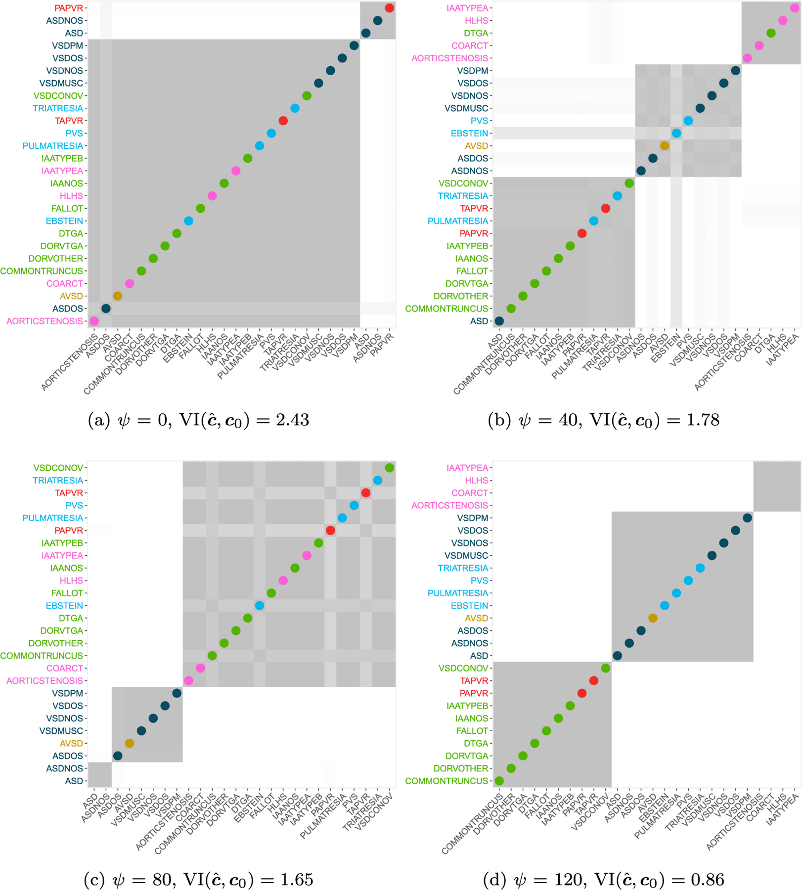
Posterior allocation matrices obtained using the CP process with a DP (α = 1) prior for different values of ψ ∈ {0, 40, 80, 120}. On the y-axis labels are colored according base grouping information c₀, with dots on the diagonal highlighting differences between c₀ and the estimated partition ĉ.

Details on the results for each of the estimated models are given in the Supplementary Material (Figures 3–7) and summarized here. Figure 11 shows a heatmap of the mean posterior log odds-ratios for increasing values of the penalization parameter ψ, with dots indicating significant values according to a 95% credibility interval. In general, the sign of the effects does not change for most of the exposure factors across the different clusterings. Figure 11 focuses on pharmaceutical use in the period from 1 month before the pregnancy and 3 months during, along with some exposures related to maternal behavior and health status.

Figure 11:

Comparison of significant odds ratio under ψ ∈ {0, 40, 80, 120, ∞} for some exposure factors and 4 selected heart defects in 4 different groups under c₀. Dots are in correspondence of significant mean posterior log-odds ratios (log-OR) at 95% with red encoding risk factors (log-OR > 0) and green protective factors (log-OR < 0).

We found consistent results for known risk factors for CHD in general, including diabetes (Correa et al., 2008) and obesity (Waller et al., 2007). The positive association between nausea and positive outcomes is likely due to the fact that nausea is indicative of a healthy pregnancy, and is consistent with prior literature (Koren et al., 2014). The association between the use of SSRIs and pulmonary atresia was also reported in Reefhuis et al. (2015). It is worth noticing that estimates obtained under the DP prior are less consistent with prior work. In particular, there are apparent artifacts such as the protective effect of alcohol consumption related to defects in the bigger cluster, which is mitigated from an informed borrowing across the defects. On the other side, estimates under separate models for AVSD or PAPVR, which corresponds to 0.02% and 0.01% of cases respectively, show how a separate analysis of cases with low prevalence misses even widely assessed risk factors, as for example diabetes.

Discussion

There is a very rich literature on priors for clustering, with almost all of the emphasis on exchangeable approaches, and a smaller literature focused on including dependence on known features (e.g. covariates, temporal or spatial structure). The main contribution of this article is to propose what is seemingly a first attempt at including prior information on an informed guess at the clustering structure. We were particularly motivated by a concrete application to a birth defects study in proposing our method, based on shrinking an initial clustering prior towards the prior guess.

Our approach is conceptually quite general and represents a first attempt to include this sort of prior information in clustering. However, we recognize that the proposed prior calibration does not allow a straightforward scaling when the number of objects is much larger than the N = 26 considered in the motivating birth defects application. This is due to a combinatorial explosion as N increases which leads to an inevitable deterioration of our prior calibration algorithm. For larger N, one can consider results from the prior calibration approach as providing a reasonable lower bound for ψ, with several higher values also considered in data analyses. An immediate direction of future research considers improving our prior calibration algorithm, by relying on more efficient sampling methods on discrete combinatorial spaces, with promising directions given in the recent works of Arratia and DeSalvo (2016) and DeSalvo (2017).

Although our proposed CP process may in principle accommodate hyperprior distributions for the Dirichlet and Pitman-Yor process parameters, a limitation is in that the prior calibration directly depends on such parameters, making the implementation difficult when hyperpriors are used. For example, if a prior is put on the hyperparameters of the baseline EPPF, then the calibration for ψ has to be performed at each MCMC step, conditionally on the value of the EPPF’s hyperparameters, unless one integrates over the hyperparameters’ distribution. We are considering the alternative of a prior distribution on ψ, although the corresponding posterior leads to an intractable normalizing constant. Possible options to address this issue may be to consider a direct approximation for the constant as in Vitelli et al. (2018), or to explore specialized MCMC algorithms for doubly intractable problems in which the likelihood involves an intractable normalizing constant (Murray et al., 2006; Møller et al., 2006; Rao et al., 2016).

There are many immediate interesting directions for future research. One thread pertains to developing better theoretical insight and analytical tractability into the new class of priors. For existing approaches, such as product partition models and Gibbs-type partitions, there is a substantial literature providing simple forms of prediction rules and other properties. It is an open question whether such properties can be modified to our new class. This may yield additional insight into the relative roles of the base prior, centering value and hyperparameters in controlling the behavior of the prior and its impact on the posterior. Another important thread relates to applications of the proposed framework beyond the setting in which we have an exact guess at the complete clustering structure. In many cases, we may have an informed guess or initial clustering in a subset of the objects under study, with the remaining objects (including future ones) completely unknown. Conceptually the proposed approach can be used directly in such cases, and also when one has different types of prior information on the clustering structure than simply which objects are clustered together.

References

- Arratia R and DeSalvo S (2016). “Probabilistic divide-and-conquer: a new exact simulation method, with integer partitions as an example.” Combinatorics, Probability and Computing, 25(3): 324–351. MR3482658. doi: 10.1017/S0963548315000358. 327 [DOI] [Google Scholar]
- Barrientos AF, Jara A, Quintana FA, et al. (2012). “On the support of MacEachern’s dependent Dirichlet processes and extensions.” Bayesian Analysis, 7(2): 277–310. MR2934952. doi: 10.1214/12-BA709. 302 [DOI] [Google Scholar]
- Barry D and Hartigan JA (1992). “Product partition models for change point problems.” The Annals of Statistics, 260–279. MR1150343. doi: 10.1214/aos/1176348521. 303 [DOI]
- Blei DM and Frazier PI (2011). “Distance dependent Chinese restaurant processes.” Journal of Machine Learning Research, 12(Aug): 2461–2488. MR2834504. 303 [Google Scholar]
- Botto LD, Lin AE, Riehle-Colarusso T, Malik S, Correa A, and Study NBDP (2007). “Seeking causes: classifying and evaluating congenital hearth defects in etiologic studies.” Birth Defects Research Part A: Clinical and Molecular Teratology, 79(10): 714–727. 319 [DOI] [PubMed] [Google Scholar]
- Caron F, Davy M, Doucet A, Duflos E, and Vanheeghe P (2006). “Bayesian inference for dynamic models with Dirichlet process mixtures” In International Conference on Information Fusion. Florence, Italy. MR2439814. doi: 10.1109/TSP.2007.900167. 302 [DOI] [Google Scholar]
- Casella G, Moreno E, Girón FJ, et al. (2014). “Cluster analysis, model selection, and prior distributions on models.” Bayesian Analysis, 9(3): 613–658. MR3256058. doi: 10.1214/14-BA869. 306 [DOI] [Google Scholar]
- Correa A, Gilboa SM, Besser LM, Botto LD, Moore CA, Hobbs CA, Cleves MA, Riehle-Colarusso TJ, Waller DK, Reece EA, et al. (2008). “Diabetes mellitus and birth defects.” American Journal of Obstetrics and Gynecology, 199(3): 237.e1–237.e9. 324 [DOI] [PMC free article] [PubMed] [Google Scholar]
- Dahl DB, Day R, and Tsai JW (2017). “Random partition distribution indexed by pairwise information.” Journal of the American Statistical Association, 112(518): 721–732. MR3671765. doi: 10.1080/01621459.2016.1165103. 303 [DOI] [PMC free article] [PubMed] [Google Scholar]
- Davey BA and Priestley HA (2002). Introduction to Lattices and Order Cambridge University Press. MR1902334. doi: 10.1017/CBO9780511809088. 303 [DOI] [Google Scholar]
- De Blasi P, Favaro S, Lijoi A, Mena RH, Prünster I, and Ruggiero M (2015). “Are Gibbs-type priors the most natural generalization of the Dirichlet process?” IEEE Transactions on Pattern Analysis and Machine Intelligence, 37(2): 212–229. 302 [DOI] [PubMed] [Google Scholar]
- De Iorio M, Müller P, Rosner GL, and MacEachern SN (2004). “An ANOVA model for dependent random measures.” Journal of the American Statistical Association, 99(465): 205–215. MR2054299. doi: 10.1198/016214504000000205. 302 [DOI] [Google Scholar]
- DeSalvo S (2017). “Improvements to exact Boltzmann sampling using probabilistic divide-and-conquer and the recursive method.” Pure Mathematics and Applications, 26(1): 22–45. MR3674129. doi: 10.1515/puma-2015-0020. 327 [DOI] [Google Scholar]
- Dobiński G (1877). “Summirung der Reihe für m = 1,2,3,4,…” Archiv der Mathematik und Physik, 61: 333–336. 317 [Google Scholar]
- Dunson DB and Park J-H (2008). “Kernel stick-breaking processes.” Biometrika, 95(2): 307–323. MR2521586. doi: 10.1093/biomet/asn012. 302 [DOI] [PMC free article] [PubMed] [Google Scholar]
- Fall MD and Barat É (2014). “Gibbs sampling methods for Pitman-Yor mixture models.” Working paper or preprint URL https://hal.archives-ouvertes.fr/hal-00740770 313
- Ferguson TS (1973). “A Bayesian Analysis of Some Nonparametric Problems.” The Annals of Statistics, 1(2): 209–230. MR0350949. 302 [Google Scholar]
- Gelfand AE, Kottas A, and MacEachern SN (2005). “Bayesian nonparametric spatial modeling with Dirichlet process mixing.” Journal of the American Statistical Association, 100(471): 1021–1035. MR2201028. doi: 10.1198/016214504000002078. 302 [DOI] [Google Scholar]
- Gnedin A and Pitman J (2006). “Exchangeable Gibbs partitions and Stirling triangles.” Journal of Mathematical Sciences, 138(3): 5674–5685. MR2160320. doi: 10.1007/s10958-006-0335-z. 302 [DOI] [Google Scholar]
- Griffin JE and Steel MF (2006). “Order-based dependent Dirichlet processes.” Journal of the American Statistical Association, 101(473): 179–194. MR2268037. doi: 10.1198/016214505000000727. 302 [DOI] [Google Scholar]
- Hartigan J (1990). “Partition models.” Communications in Statistics – Theory and Methods, 19(8): 2745–2756. MR1088047. doi: 10.1080/03610929008830345. 303 [DOI] [Google Scholar]
- Jensen ST and Liu JS (2008). “Bayesian clustering of transcription factor binding motifs.” Journal of the American Statistical Association, 103(481): 188–200. MR2420226. doi: 10.1198/016214507000000365. 306 [DOI] [Google Scholar]
- Knuth DE (2005). The Art of Computer Programming. Generating all combinations and partitions Addison-Wesley. MR0478692. 315 [Google Scholar]
- Koren G, Madjunkova S, and Maltepe C (2014). “The protective effects of nausea and vomiting of pregnancy against adverse fetal outcome. A systematic review.” Reproductive Toxicology, 47: 77–80. 325 [DOI] [PubMed] [Google Scholar]
- Lin AE, Herring AH, Amstutz KS, Westgate M-N, Lacro RV, Al-Jufan M, Ryan L, and Holmes LB (1999). “Cardiovascular malformations: changes in prevalence and birth status, 1972–1990.” American Journal of Medical Genetics, 84(2): 102–110. 319 [PubMed] [Google Scholar]
- MacEachern SN (1999). “Dependent nonparametric processes.” In Proceedings of the Bayesian Section, 50–55. Alexandria, VA: American Statistical Association. 302 [Google Scholar]
- MacEachern SN (2000). “Dependent nonparametric processes.” Technical report, Department of Statistics, The Ohio State University. 302 [Google Scholar]
- MacLehose RF and Dunson DB (2010). “Bayesian semiparametric multiple shrink-age.” Biometrics, 66(2): 455–462. MR2758825. doi: 10.1111/j.1541-0420.2009.01275.x. 319 [DOI] [PMC free article] [PubMed] [Google Scholar]
- Meilă M (2007). “Comparing clusterings – an information based distance.” Journal of Multivariate Analysis, 98(5): 873–895. MR2325412. doi: 10.1016/j.jmva.2006.11.013. 303, 308 [DOI] [Google Scholar]
- Møller J, Pettitt AN, Reeves R, and Berthelsen KK (2006). “An efficient Markov chain Monte Carlo method for distributions with intractable normalising constants.” Biometrika, 93(2): 451–458. MR2278096. doi: 10.1093/biomet/93.2.451. 327 [DOI] [Google Scholar]
- Monjardet B (1981). “Metrics on partially ordered sets – A survey.” Discrete Mathematics, 35(1): 173–184. Special Volume on Ordered Sets. MR0620670. doi: [Google Scholar]
- Müller P, Quintana F, and Rosner GL (2011). “A product partition model with regression on covariates.” Journal of Computational and Graphical Statistics, 20(1): 260–278. MR2816548. doi: 10.1198/jcgs.2011.09066. 303 [DOI] [PMC free article] [PubMed] [Google Scholar]
- Murray I, Ghahramani Z, and MacKay DJC (2006). “MCMC for doubly-intractable distributions” In Proceedings of the 22nd Annual Conference on Uncertainty in Artificial Intelligence (UAI-06), 359–366. AUAI Press. 327 [Google Scholar]
- Neal RM (2000). “Markov chain sampling methods for Dirichlet process mixture models.” Journal of Computational and Graphical Statistics, 9: 249–265. MR1823804. doi: 10.2307/1390653. 313, 314 [DOI] [Google Scholar]
- Nijenhuis A and Wilf HS (2014). Combinatorial Algorithms: for Computers and Calculators Elsevier. MR0510047. 315 [Google Scholar]
- Paganin S, Herring AH, Olshan AF, Dunson DB, and The National Birth Defects Prevention Study (2020). “Centered Partition Processes: Informative Priors for Clustering – Supplementary Material.” Bayesian Analysis doi: 10.1214/20-BA1197SUPP. 303 [DOI] [PMC free article] [PubMed]
- Park J-H and Dunson DB (2010). “Bayesian generalize product partition models.” Statistica Sinica, 20: 1203–1226. MR2730180. 303 [Google Scholar]
- Petrone S, Guindani M, and Gelfand AE (2009). “Hybrid Dirichlet mixture models for functional data.” Journal of the Royal Statistical Society: Series B (Statistical Methodology), 71(4): 755–782. MR2750094. doi: 10.1111/j.1467-9868.2009.00708.x. 302 [DOI] [Google Scholar]
- Pitman J (1995). “Exchangeable and partially exchangeable random partitions.” Probability Theory and Related Fields, 102(2): 145–158. MR1337249. doi: 10.1007/BF01213386. 302 [DOI] [Google Scholar]
- Pitman J (1997). “Some probabilistic aspects of set partitions.” The American Mathematical Monthly, 104(3): 201–209. MR1436042. doi: 10.2307/2974785. 317 [DOI] [Google Scholar]
- Pitman J and Yor M (1997). “The two-Parameter Poisson-Dirichlet distribution derived from a stable subordinator.” The Annals of Probability, 25(2): 855–900. MR1434129. doi: 10.1214/aop/1024404422. 302 [DOI] [Google Scholar]
- Polson NG, Scott JG, and Windle J (2013). “Bayesian inference for logistic models using Pólya-Gamma latent variables.” Journal of the American Statistical Association, 108(504): 1339–1349. MR3174712. doi: 10.1080/01621459.2013.829001. 321 [DOI] [Google Scholar]
- Rao V, Lin L, and Dunson DB (2016). “Data augmentation for models based on rejection sampling.” Biometrika, 103(2): 319–335. MR3509889. doi: 10.1093/biomet/asw005. 327 [DOI] [PMC free article] [PubMed] [Google Scholar]
- Rasmussen SA, Olney RS, Holmes LB, Lin AE, Keppler-Noreuil KM, and Moore CA (2003). “Guidelines for case classification for the National Birth Defects Prevention Study.” Birth Defects Research Part A: Clinical and Molecular Teratology, 67(3): 193–201. 318 [DOI] [PubMed] [Google Scholar]
- Reefhuis J, Devine O, Friedman JM, Louik C, and Honein MA (2015). “Specific SSRIs and birth defects: Bayesian analysis to interpret new data in the context of previous reports.” British Medical Journal, 351. 325 [DOI] [PMC free article] [PubMed]
- Rodriguez A and Dunson DB (2011). “Nonparametric Bayesian models through probit stick-breaking processes.” Bayesian Analysis, 6(1). MR2781811. doi: [DOI] [PMC free article] [PubMed] [Google Scholar]
- Rossi G (2015). “Weighted paths between partitions.” arXiv preprint URL https://arxiv.org/abs/1509.01852 308
- Scarpa B and Dunson DB (2009). “Bayesian Hierarchical Functional Data Analysis Via Contaminated Informative Priors.” Biometrics, 65(3): 772–780. MR2649850. doi: 10.1111/j.1541-0420.2008.01163.x. 302 [DOI] [PubMed] [Google Scholar]
- Sethuraman J (1994). “A constructive definition of Dirichlet priors.” Statistica Sinica, 4(2): 639–650. MR1309433. 302 [Google Scholar]
- Smith AN and Allenby GM (2019). “Demand Models With Random Partitions.” Journal of the American Statistical Association doi: 10.1080/01621459.2019.1604360. 303 [DOI]
- Stam A (1983). “Generation of a random partition of a finite set by an urn model.” Journal of Combinatorial Theory, Series A, 35(2): 231–240. MR0712107. doi: 10.1016/0097-3165(83)90009-2. 316, 317 [DOI] [Google Scholar]
- Stanley RP (1997). Enumerative combinatorics Vol. 1. Cambridge University Press. MR1442260. doi: 10.1017/CBO9780511805967. 303 [DOI] [Google Scholar]
- Vinh NX, Epps J, and Bailey J (2010). “Information theoretic measures for clusterings comparison: variants, properties, normalization and correction for chance.” Journal of Machine Learning Research, 11(Oct): 2837–2854. MR2738784. 308 [Google Scholar]
- Vitelli V, Øystein Sørensen, Crispino M, Frigessi A, and Arjas E (2018). “Probabilistic preference learning with the Mallows rank model.” Journal of Machine Learning Research, 18(158): 1–49. MR3813807. 327 [Google Scholar]
- Wade S and Ghahramani Z (2018). “Bayesian cluster analysis: point estimation and credible balls (with Discussion).” Bayesian Analysis, 13(2): 559–626. MR3807860. doi: 10.1214/17-BA1073. 303, 308 [DOI] [Google Scholar]
- Waller DK, Shaw GM, Rasmussen SA, Hobbs CA, Canfield MA, Siega-Riz A-M, Gallaway MS, and Correa A (2007). “Prepregnancy obesity as a risk factor for structural birth defects.” Archives of Pediatrics & Adolescent Medicine, 161(8): 745–750. 324 [DOI] [PubMed] [Google Scholar]
- Wilson R and Watkins JJ (2013). Combinatorics: Ancient & Modern OUP Oxford. MR3204727. doi: 10.1093/acprof:oso/9780199656592.001.0001. 304 [DOI] [Google Scholar]
- Yoon PW, Rasmussen SA, Lynberg MC, Moore CA, Anderka M, Carmichael SL, Costa P, Druschel C, Hobbs CA, Romitti PA, Langlois PH, and Edmonds LD (2001). “The National Birth Defects Prevention Study.” Public Health Reports, 116: 32–40. 318 [DOI] [PMC free article] [PubMed] [Google Scholar]