Assessment of Non-Occupational 1,4-Dioxane Exposure Pathways from Drinking Water and Product Use

Abstract

1,4-Dioxane is a persistent and mobile organic chemical that has been found by the United States Environmental Protection Agency (USEPA) to be an unreasonable risk to human health in some occupational contexts. 1,4-Dioxane is released into the environment as industrial waste and occurs in some personal-care products as an unintended byproduct. However, limited exposure assessments have been conducted outside of an occupational context. In this study, the USEPA simulation modeling tool, Stochastic Human Exposure and Dose Simulator-High Throughput (SHEDS-HT), was adapted to estimate the exposure and chemical mass released down the drain (DTD) from drinking water consumption and product use. 1,4-Dioxane concentrations measured in drinking water and consumer products were used by SHEDS-HT to evaluate and compare the contributions of these sources to exposure and mass released DTD. Modeling results showed that compared to people whose daily per capita exposure came from only products (2.29 × 10⁻⁷ to 2.92 × 10⁻⁷ mg/kg/day), people exposed to both contaminated water and product use had higher per capita median exposures (1.90 × 10⁻⁶ to 4.27 × 10⁻⁶ mg/kg/day), with exposure mass primarily attributable to water consumption (75–91%). Last, we demonstrate through simulation that while a potential regulatory action could broadly reduce DTD release, the proportional reduction in exposure would be most significant for people with no or low water contamination.

Graphical abstract

1. INTRODUCTION

1,4-Dioxane is a chemical of growing concern internationally and at the state and national levels in the United States.¹ Historically used as a chemical stabilizer of chlorinated solvents,² its major industrial uses today include as a processing aid, as a component of functional fluids, and as a laboratory chemical.³ It is also generated as an unintended byproduct during the ethoxylation and subsequent sulfation of ingredients (e.g., surfactants) that are found in several consumer products, such as detergents.² In both cases, unintentionally produced 1,4-dioxane can be released into the environment through wastewater, through either industrial discharge or down-the-drain (DTD) discharge from consumers following the use of its products. 1,4-Dioxane has been proposed as a “persistent, mobile, and toxic” compound per criteria developed for the European Union’s Registration, Evaluation, Authorisation, and Restriction of Chemicals (REACH) legislation.⁴ It is resistant to biodegradation, highly mobile in surface water (SW) and groundwater (GW) and is not effectively removed by typical wastewater and drinking water treatment processes.^4,5 As such, 1,4-dioxane release into the environment can lead to its accumulation in drinking water sources. Effective methodologies for the detection of 1,4-dioxane in different media have been developed,^2,6 and surveys have demonstrated that 1,4-dioxane is widely present in both drinking water and wastewater effluent across all 50 US states⁷ and some European countries.⁸

Acute and chronic toxicity points of departure have been noted for 1,4-dioxane in several organ systems in laboratory animals, and exposure to humans has been demonstrated from multiple pathways.^2,3 It has been shown to cause cancer in laboratory animals and was found by the United States Environmental Protection Agency (USEPA) to pose an unreasonable risk to workers in some occupational contexts.³

Despite these concerns, important knowledge gaps exist in 1,4-dioxane exposure. While investigations into occupational exposures have been documented since the 1970s,^9,10 non-occupational exposures have been mostly inferred from 1,4-dioxane concentrations in water sources and wastewater effluent.^2,3,5,6 Non-occupational exposure (simply “exposure” hereafter) occurs through two primary pathways: consumption of contaminated drinking water and through inhalation and dermal absorption during the use of personal care or cleaning products containing 1,4-dioxane.¹⁰ Through end-of-life disposal by consumers, product use can add to wastewater concentrations. This can then contribute back to drinking water contamination through the discharge of effluent into SW,^6,11 leaching into ground water, or the reuse of treated wastewater as drinking water supplies (Figure 1).^12,13 Although industrial wastewater releases are likely a major source of 1,4-dioxane contamination,¹¹ product use may be a significant source of wastewater contamination in places where industrial releases of 1,4-dioxane would not be expected.

Figure 1.

Exposure scenario for 1,4-dioxane. People (A) are exposed to 1,4-dioxane through two pathways, including contaminated drinking water (B) and ethoxylated ingredients in products (C). These two sources can then indirectly contaminate wastewater (D) via down-the-drain activity. Meanwhile, SW and GW (E) can be contaminated through industrial effluent and inadvertent spill releases (F) and wastewater effluent streams. Finally, both contaminated SW/ground water and treated wastewater reused as drinking water can eventually result in contaminated drinking water.

This study hypothesized that the consumer use of products containing ethoxylated ingredients may be an important source of non-occupational 1,4-dioxane exposure and wastewater contamination relative to 1,4-dioxane contaminated drinking water. To investigate this hypothesis, we developed a novel computational workflow that incorporated the USEPA’s Stochastic Human Exposure and Dose Simulator–High Throughput (SHEDS-HT)¹⁴ exposure simulation tool. Using this workflow, we used publicly available data to estimate exposure, mass released DTD, and proportional contributions from different sources of 1,4-dioxane. We also evaluated model predictions against measured data and investigated the effects of a mitigation strategy on exposure and mass released DTD. Together, this work bridges important knowledge gaps in our understanding of non-occupational exposure pathways to 1,4-dioxane.

2. METHODS

2.1. Scientific Workflow.

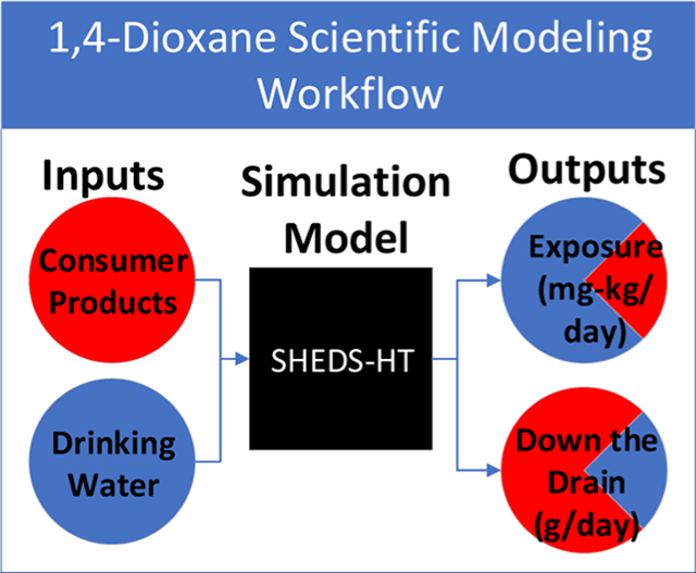
The general workflow for this study (Figure 2) included (1) the assembly and preparation of data for use in exposure modeling, (2) executing exposure simulation algorithms and processing outputs for analyses, and (3) conducting analyses. The data assembly step was conducted manually, but the latter steps were conducted using a series of interconnected computer scripts in the R programming language.¹⁵ At the core of this workflow is the SHEDS-HT platform,¹⁴ which uses information about product composition and use to provide probabilistic estimates of chemical exposure at the population level. It does this by aggregating single-day, simulated exposures for a large synthetic sample population generated from US Census information, including age and gender.¹⁴ As the underlying exposure algorithms (see Section S1.1) are generally similar to those used in a recent USEPA risk evaluation of 1,4-dioxane,³ SHEDS-HT was expected to reasonably estimate exposure here. For this study, we customized SHEDS-HT (see Section 2.3 for details) to simulate non-occupational, 1,4-dioxane exposures through two pathways: the use of contaminated drinking water and contaminated consumer products. Primary outputs included aggregate human exposure (in an absorbed dose in mg/kg/day) and the mass of chemicals released DTD per day (in g/day).

Figure 2.

Computational workflow diagram. The workflow contains three main steps (headed by black boxes), including (1) assembling model inputs [water (light blue boxes) and consumer products (red boxes)], (2) running model inputs through modular exposure scenario algorithms (red or blue, as appropriate) and collecting and processing exposure modeling outputs (purple boxes), and (3) analysis of model outputs (dark blue boxes). The simulations run by SHEDS-HT and the analyses of their outputs were dictated by the study design. Black arrows demonstrate the flow of information from one step to the next.

2.2. Model Inputs.

To estimate human exposure and mass released DTD, SHEDS-HT requires knowledge about chemical concentration, chemical prevalence, product use, food and water consumption, and a variety of exposure factors and use parameters. Unless otherwise described below, default values provided within SHEDS-HT were used. Parameter values for all model simulations are included in Section S3.

2.2.1. Drinking Water.

For this analysis, we consider only drinking water provided through a public drinking water source, that is, tap water. Estimating tap water ingestion required three parameters: the prevalence of 1,4-dioxane contamination in tap water (prevalence_water), the concentration of 1,4-dioxane in contaminated tap water (conc_water), and the amount of tap water ingested. The first two were derived from monitoring data collected as part of the implementation of the Third Unregulated Contaminant Monitoring Rule (UCMR3).¹⁶ The UCRM3 was a program of the USEPA in which a set of contaminants that are of concern but unregulated were monitored in drinking water from 2013 to 2015. As part of this program, 1,4-dioxane was monitored twice a year at 4913 public water systems across all 50 US states. The amount of tap water ingested was derived from the National Health and Nutrition Examination Survey (NHANES) What-We-Eat-in-America¹⁷ survey.

The parameters for estimates of 1,4-dioxane mass released DTD in tap water were made using gross per capita water usage data.¹⁸ Included implicitly were quantities for major contributing activities such as bathing, handwashing, washing dishes, and doing laundry. Per capita quantities of ingested tap water based on NHANES data were a very small percentage of average daily water usage in the United States (<1%) and were not subtracted from the gross total considered for mass released DTD. See Section S1.2.1 for a detailed description of the development of tap water parameters.

2.2.2. Consumer Products.

To estimate human exposure to 1,4-dioxane from product use, we considered concentrations in six product classes (shampoo, body wash, hand soap, laundry detergent, manual dish detergent, and bubble bath) identified in three studies.^19–21 Several parameters were needed to estimate the exposure and mass released DTD from consumer product use. One of these parameters was the concentration of 1,4-dioxane in different consumer products (conc_products). This was derived from literature-based values measured using gas chromatography with mass spectrometry.^19–21 Another parameter was the prevalence of 1,4-dioxane in different product classes (prevalence_products), for which we explicitly considered a range of values as part of our factorial analyses (see Section 2.4.1 for more details). For the remaining parameters (e.g., product use frequency, product use duration, product use mass, etc.), we used either SHEDS-HT default values or values from the Exposure Factors Handbook. See Sections S1.2.2 for a detailed description of the processing of consumer product data and S2.2 for the assembled consumer product data.

2.3. Model Algorithms.

To model human exposure from contaminated tap water, we used the Food Residue scenario of SHEDS-HT to capture only the dietary pathway. This is because the significantly lower values of 1,4-dioxane concentrations in water relative to the concentrations in products (≈3–4 orders of magnitude lower, see Section S3) made the potential for significant inhalation and dermal exposure from water relatively small. Exposure to 1,4-dioxane from consumer products was modeled using the dermal and inhalation modules of the Direct Product Exposure scenario. Incidental ingestion exposure through hand-to-mouth contact was also included with the dermal pathway module. We used the DTD module to model mass released DTD from both previously contaminated tap water and consumer product use. See Section S2.3 for descriptions of the underlying exposure equations used in each module described.

Three main adjustments were made to the SHEDS-HT base coding to better reflect the assumptions of the exposure scenarios. In brief, these modifications included (1) coupling the tap water concentrations used to estimate exposure and mass released DTD for a given person (decoupled by default); (2) better aligning the frequency of handwashing and bathing (which are by default de-coupled from product use) to a person’s use of soap and bath products, respectively; and (3) preventing the unlikely scenario of a person using multiple kinds of the same product type (e.g., gel and liquid laundry detergent) in the same day. As part of the workflow, a customized code was also developed to enable the implementation of multiple scenarios and to enable the tracking of simulated individuals over multiple runs. See Section S1.3 for additional details on these modifications.

SHEDS-HT uses a Monte Carlo sampling approach to stochastically assign values to the parameters of exposure equations by probabilistically drawing samples from user-specified distributions. See Section S1.4 for details on this process and Section S3 for distributions assigned to each parameter.

2.4. Simulations and Analyses.

2.4.1. Factorial Simulation Study: Comparing the Water Source and Product Use as Drivers of Exposure and Mass Released DTD.

An individual’s exposure to 1,4-dioxane and mass released DTD is expected to vary based on their water source and use of consumer products. To capture some of this variability in our assessment and to compare the relative contributions of the two pathways (i.e., tap water use and product use) to the two outputs, we conducted a factorial analysis. The first of three comparative factors, water source, reflected variations in distributions of 1,4-concentrations in tap water (i.e., conc_water) depending upon whether local water was supplied by GW, SW, or a mixture of GW and SW (MX).

The second factor, geographic scale, reflected regional variations [the United States or the state of California (CA)] of water source data. This factor was included to serve as a comparison of conditions between the United States at large and a subset of water systems. California was selected as a data-rich case for which the available UCMR3 data included a large number of municipal water systems (455) across all three water source types at reasonably similar proportions (GW: 62.4%, SW: 32.1%, MX: 5.3%) as the national level (GW: 50.6%, SW: 47.2%, MX: 2.0%). The state government is also currently considering the implementation of consumer product regulations to reduce the risk from DTD releases of 1,4-dioxane (https://dtsc.ca.gov/scp/1-4-dioxane/; accessed August 23, 2021) and thus would be informed by this research.

The third factor was the prevalence of 1,4-dioxane occurring in products (prevalence_products) and described how likely a product user is to encounter 1,4-dioxane in a purchased product (e.g., brand X) of a given class (e.g., shampoo). There is considerable uncertainty about this parameter for different products, so we considered it here as a factor with two levels: low and high. See Section S1.5 for a description of the derivation of the high and low bounds for prevalence_products. Together, the three factors resulted in 12 factorial combinations.

We performed two sets of statistical analyses. First, analysis of variance (ANOVA) was used to analyze how outputs were affected by source, scale, and prevalence_products. By making the assumption that non-detection of 1,4-dioxane (defined as any concentration below the minimum reporting limit of 0.07 μg/L) in water equated to no exposure from tap water, distinct populations emerged. These included: (1) the entire sample population (“total”), (2) the subset of people exposed only through products (“products only”), and (3) the subset of people exposed through both products and water (“both”). We conducted separate, 3-way, fixed-effects ANOVAs for each population. An interaction term between scale and source was included in statistical models, but interaction terms with prevalence_products were not. This is because the effects of prevalence_products on exposure and mass released DTD would be expected to be additive to scale and source. ANOVA assumptions of homoskedasticity and the normal distribution of residuals were visually assessed and determined to be reasonably met. To help with the interpretation of factorial effects, we calculated the metric η_partial² for treatment factors as

$${{\eta }_{\text{partial}}}^2=\frac{{\text{SS}}_{\text{treatment}}}{{\text{SS}}_{\text{treatment}}+{\text{SS}}_{\text{error}}}$$ (1)

in which SS_treatment = the sum of squares associated with a factor, and SS_error is the error sum of squares of the ANOVA model. η_partial² provides an estimate of the total proportion of variance of the dependent variable (i.e., human exposure or mass released DTD) that is due to an independent variable after accounting for the variance of other variables.²²

Second, we conducted analyses to characterize how the two pathways (i.e., tap water use and consumer product use) proportionally contributed to exposure and mass released DTD. For the “both” population, we first determined the majority contributor (i.e., tap water or consumer products) to exposure and mass released DTD. Then, Beta regression was used to model how the included factors influenced the majority contributor to exposure and mass released DTD.²³ We used Cohen’s D as a measure of effect sizes between factorial levels, calculated with the R package “effectsize”.²⁴ We did not conduct a corresponding statistical analysis for the products only and total populations. For the former, no individuals are exposed to tap water. For the latter, the high proportion of individuals not exposed to tap water in most groups makes the meaningful interpretation of statistical comparison difficult. Therefore, we present summary statistics only for the total population.

2.4.2. Model Evaluation.

1,4-Dioxane is rapidly metabolized in the blood into 2-(2-hydroxyethoxy)acetic acid, which is also excreted relatively rapidly [half-life (t_1/2) = 3.5 h].²⁵ Therefore, there are no available biomonitoring data to evaluate exposure estimates. Instead, the model was evaluated by comparing estimates of mass released DTD to concentrations detected at wastewater treatment plants (WWTPs). To translate mass released DTD predictions from SHEDS-HT to expected wastewater loading, we used the Web-based ISTREEM tool.²⁶ This freely available tool (currently hosted by the American Cleaning Institute) predicts concentrations of chemicals at WWTPs (influent and effluent) by using municipal flow rates, city population information, and per capita mass released DTD in a basic pollutant loading model (i.e., daily wastewater concentration = total mass released DTD/total municipal flow). Using this tool, and assuming no reduction of 1,4-dioxane from treatment (i.e., influent = effluent concentration),⁵ we predicted expected concentrations (μg/L) of 1,4-dioxane in wastewater effluent at 142 WWTPs in CA (reported to serve 14.2 million people) and 13,245 WWTPs in the United States overall (reported to serve 182.62 million people) that are listed in the ISTREEM database. This accounts for WWTPs that serve about 36% and 55% of the populations of CA and the United States, respectively. See Section S1.6 for additional details on the methods used to convert DTD release to wastewater effluent concentrations. At the US geographic scale, measured data included 1,4-dioxane concentrations collected in wastewater effluent at 40 WWTPs across the United States.⁵ There was a method detection limit (MOD) of 0.1 μg/L, with no samples found below this limit. At the CA geographic scale, we used a collection of wastewater effluent concentrations from 17 wastewater treatment and water reclamation facilities in CA, collected from 2013 to 2015.²⁷ The MDL values ranged from 0.04 to 0.59 μg/L. We converted values less than the MDL to half the value of the MDL. We compared our projected wastewater concentrations of each factorial combination against the measured data at the corresponding geographic scale using descriptive statistics.

2.4.3. Simulated Mitigation Strategy.

A potential mitigation strategy to lower exposures from chemicals in products is to reduce the total concentration of a chemical in products (i.e., conc_products) below a set threshold. The state of CA has proposed a 1 mg/L threshold for 1,4-dioxane in consumer products, and the state of New York has stipulated a legal limit of 1 mg/L in personal care and cleaning products by 2023.¹ To simulate the effect of this intervention strategy on human exposure and mass released DTD, we investigated scenarios in which the upper limit of the available distribution of conc_products was truncated to 1 mg/L. In the data set assembled for this study (see Section S2.2), concentrations measured in consumer products ranged from 0.22 to 35 mg/L, with a mean and standard deviation of 3.098 ± 4.42 mg/L. The range used here may actually be conservative, as recent lab analyses by the California Department of Environmental Protection (data not available for this work) showed that 1,4-dioxane concentrations can reach as high as 132 mg/L in personal care and cleaning products intended to be washed DTD after use.²⁸ In the simulated scenarios, we considered 1,4-dioxane concentrations at the CA scale from all source types (GW, SW, and MX) but assumed only a high prevalence_products. We used Student’s t tests to compare how human exposure and mass released DTD varied between the simulated threshold scenario and the non-threshold scenarios described above. A separate t test was used to address each population (total, products only, and both), followed by the calculation of percentage reductions in mean exposure and mass released DTD when a threshold is applied. Because sample populations were arbitrarily large (e.g., we used SHEDS-HT default of 10,000 per population), Bonferroni corrections were not made to p-values.

3. RESULTS

3.1. Factorial Simulation Results.

Due to the large sample size of simulated populations, most statistical tests were found to be statistically significant at the α = 0.050 level. Therefore, we report factorial group medians in the main text for discussion context and primarily limit our statistical discussion to effect sizes. Please see the Supporting Information for tabulated descriptive statistics for simulations of all factorial groups (Sections S2.6 and S2.8) and for full statistical details (Sections S2.7 and S2.9) of the results presented below.

3.1.1. Human Exposure.

Estimates of median absorbed doses ranged across all factorial groups from 2.71 × 10⁻⁷ to 7.47 × 10⁻⁷ mg/kg/day for the total population, 2.29 × 10⁻⁷ to 2.92 × 10⁻⁷ mg/kg/day for the product’s only population, and from 1.90 × 10⁻⁶ to 4.27 × 10⁻⁶ mg/kg/day for the both population. Using η_partial² benchmarks of 0.010, 0.060 and 0.14 for small, medium, and large sizes,²² effect sizes for all factors were minor (<0.0010–0.024), with some differences emerging by factor. Median exposures tended to increase with source from SW (total: 2.98 × 10⁻⁷ mg/kg/day, both: 2.01 × 10⁻⁶ mg/kg/day) to GW (total: 3.57 × 10⁻⁷ mg/kg/day, both: 3.17 × 10⁻⁷ mg/kg/day) to MW (total: 5.00 × 10⁻⁷ mg/kg/day, both: 4.13 × 10⁻⁶ mg/kg/day) across the total and both populations. This represented small-to-moderate effect sizes of source on exposure (total η_partial² = 0.020, both η_partial² = 0.024). In contrast, exposure was only slightly higher at the CA geographic scale than the US geographic scale for the total and both populations (η_partial² = 0.0080–0.0020), and there was no statistically significant difference in exposure between high prevalence_products and low prevalence_products conditions. Thus, although minor, water source had the largest impacts on exposure relative to the population variance introduced through the SHEDS-HT Monte Carlo sampling process.

Interestingly, although the use of MW resulted in the highest median exposure, 1,4-dioxane concentrations (i.e., conc_water) in GW (0.41 μg/L) were higher than in MW (0.29 μg/L) or SW (0.23 μg/L) (see Section S3.4). The reason for this seeming inconsistency is that GW concentration data had higher coefficients of variation (CA: 1.58, US: 1.59), that is, were more variable, than MW concentration data (CA: 0.23, US: 0.33). Because SHEDS-HT assigned the values of water source concentration to individuals by random sampling from the lognormal distribution, the more variable GW data resulted in a larger number of individuals assigned to lower concentrations, pulling the median down. See Section S2.6 for summary statistics for each factorial group and Section S2.7A for complete statistical details.

3.1.2. Pathway Contribution to Human Exposure: Proportion due to Tap Water Contamination.

For the total population, the relatively low prevalence_water for most source types resulted in the median proportion of exposure due to water contamination to be 0.00 for all factorial combinations (Figure 3A). Although the proportions of exposure mass varied within factorial groups (standard deviations ranged from 0.11 to 0.43), the lack of variance around the median obscured interpretable patterns of how the water pathway contributed to overall exposure patterns of the total population. In contrast, the consumption of contaminated tap water was the main pathway for human exposure for all factorial groups of the both population, accounting for a proportion of exposure mass ranging from a mean low of 0.76 (scale: US, source: SW, prevalence_products: high) to a mean high of 0.91 (scale: CA, source: MW, prevalence_products: low) (Figure 3B).

Figure 3.

Proportion of human exposure due to ingestion of contaminated water across each factorial combination for (A) the total sample population (i.e., total) and (B) subset of the total sample population with both contaminated water and products (i.e., both). Geographic scale is shown on the x-axis (with CA on left, US on right), water source is indicated by color [GW = blue, SW = green, and mixed water (MX) = red], and prevalence_products is indicated by color shade (high = dark, low = light). The groups in A (e.g., GW:low) are aligned vertically with the corresponding groups in B. The population size (i.e., N) of each water source group in (A) was 10,000. The N of each water source group in (B) is shown above the figure. For convenience, the source and prevalence_products combination is listed below each group.

A Beta regression model fit to the proportion of exposure due to contaminated tap water found only significant main effects for factors (i.e., no interactions). Calculated Cohen’s D values are effect size metrics that, in this case, indicate how one level of a factor (e.g., GW) influences the proportion of exposure mass due to tap water consumption relative to another level of the same factor (e.g., SW). The largest effect sizes (D = 0.66, D = 0.36) were found through comparisons between MW (average proportion = 0.90) and SW (average proportion = 0.78) and GW (average proportion = 0.88) and SW, respectively. Conversely, only a small effect difference (D = −0.040) was found between low prevalence_products and high prevalence_products. Lastly, the effect of spatial scale was intermediate (D = 0.19), with the proportion of exposure due to contaminated water larger at the CA (0.87) scale than at the US scale (0.84). See Section S2.8 for data reported here and Section S2.9A for full statistical details.

3.1.3. Mass Released DTD.

The estimated median per capita 1,4-dioxane mass released DTD ranged across all factorial groups from 9.32 × 10⁻⁴ to 1.00 × 10⁻³ g/day for the total population, 7.91 × 10⁻⁴ to 9.60 × 10⁻⁴ g/day for the product’s only population, and from 1.28 × 10⁻³ to 1.86 × 10⁻³ g/day for the both population (Section S2.6). Effect sizes for factors across all three populations were very small, with η_partial² ≤ 0.0010 for all factors. In addition, for the both population, only prevalence_products was found to have a statistically significant effect, despite the large sample size. Thus, none of the considered factors had a meaningful effect on mass released DTD relative population variance introduced by SHEDS-HT. See Section S2.6 for summary statistics for each factorial group and Section S2.7B for complete statistical details.

3.1.4. Contribution of Pathway to Mass Released DTD: Proportion Attributable to Consumer Product Use.

The median proportion of 1,4-dioxane mass released DTD attributable to consumer products was 1.00 across all groups for the total population (Figure 4A). This result was due to the relatively low prevalence_water of contaminated water systems in the total population. Like for the human exposure scenario, this pattern obscured interpretable patterns of how consumer products contributed to mass released DTD. When considering the both population, the median proportion of mass released DTD attributable to consumer products ranged from 0.93 to 0.98 (Figure 4B). A Beta regression model fit to the data for both populations found only significant main effects, with effect sizes of factors all relatively minor (Cohen’s D ≤ |0.21|). Overall, the proportion of mass released DTD due to product use increased with the use of tap water with lower 1,4-dioxane water concentrations (e.g., at the US scale; SW) or the assumption of a higher prevalence_products. Interestingly, despite the overwhelming importance of product use to the mass of 1,4-dioxane released DTD, the effect size of prevalence_products on the proportion of mass released DTD due to product use was the smallest of the factors (Cohen’s D = 0.029). It can be concluded that for the purposes of predicting mass released DTD, the two methods of estimating product_prevalence for this study (i.e., high and low) were functionally equivalent. See Sections S2.8 and S2.9 for graphical/tabular data summaries and statistical details, respectively.

Figure 4.

Proportion of mass released DTD attributable to the use of contaminated consumer products for (A) the total aggregate population (i.e., total) and (B) the population with both contaminated water and products (i.e., both). Geographic scale is shown on the x-axis (with CA on left, US on right), water source is indicated by color [GW = blue, SW = green, and mixed water (MX) = red], and prevalence_products is indicated by color shade (high = dark, low = light). The groups in A (e.g., GW:low) are aligned vertically with the corresponding groups in B. The population size (i.e., N) of each water source group in (A) was 10,000. The N of each water source group in (B) is shown above the figure. For clarity, the source and prevalence_products combination is listed below each group.

3.2. Model Evaluation.

1,4-Dioxane concentrations projected in wastewater by ISTREEM were compared to measured concentrations (shown here as median ± standard deviation) from WWTPs at the CA scale (0.65 ± 0.618 μg/L) and from WWTPs across the United States (1.125 ± 0.60 μg/L). The medians and 95th percentile values of projected concentrations were generally higher than the measured concentrations but were within a 10-fold difference. For the CA scale groups, medians of simulated effluent data ranged from 2.42 to 5.69 μg/L, corresponding to values 3.73–8.76 times higher than the median of the CA measured data. For the US scale groups, medians of simulated effluent ranged from 2.10 to 3.74 μg/L, corresponding to values 1.87–3.33 times higher than the median of US measured data.

For the purposes of a screening-level analysis, a less than 10-fold difference between predicted and observed distributions suggests that the model was able to reasonably capture important sources of variance contributing to population-level wastewater treatment plant 1,4-dioxane concentrations. However, there are some important limitations of this evaluation worth noting. First, the list of products included in this analysis was not comprehensive (e.g., surface cleaners and paint were not included), suggesting that model-based projections of wastewater effluent concentrations would be even higher than the measured data if additional products were included. Second, measured 1,4-dioxane concentrations were collected as grab samples at various locations on very few dates (1–4). Therefore, they may not be representative of the entire range of 1,4-concentrations expected at the WWTPs sampled. Last, there is considerable uncertainty in some of the parameters used to calculate mass released DTD. Although a sensitivity analysis of the DTD module has not been conducted, a partial sensitivity analysis of human exposure predictions from SHEDS-HT showed that three corresponding parameters [mass of product applied, frequency of use, and chemical concentration (i.e., conc_products)] were particularly influential on the model output.¹⁴ Thus, better estimates of these exposure factor parameters may also improve the accuracy of both model outputs. See Sections S2.3 for listing of the SHEDS-HT DTD equations, Section S1.2.2 for a discussion of parameter sources, and Section S2.10 for full model evaluation results.

3.3. Simulated Threshold.

Imposing an upper limit of 1 mg/L on conc_products resulted in significant reductions in both human exposure and mass released DTD for all three populations of the CA high prevalence_products population subset (Table 1). For human exposure, percentage reduction from the no action scenario (i.e., threshold not imposed) to the threshold scenario ranged from a low of about a 9% (reduced from 9.23 × 10⁻⁶ to 8.38 × 10⁻⁶ mg/kg/day) for those exposed to both products and contaminated GW (i.e., both population) to a high of about 85% (reduced from 7.54 × 10⁻⁷ to 1.19 × 10⁻⁷ mg/kg/day) for the products-only population. Percentage reductions in mass released DTD ranged from 80% to 85% across all three water sources and populations. The difference in percentage reduction between human exposure and mass released DTD reflects the relative importance of contaminated tap water versus product use in the two outputs. For exposure, results suggest that the extent of the benefits of imposing a threshold would vary depending upon the population considered. Those with uncontaminated water (i.e., products-only) could potentially benefit the most directly, as it would reduce their only or primary sources of exposure. In contrast, mass released DTD may be broadly reduced by such mitigation strategy across all populations. However, as discussed in the next section, such a reduction in mass released DTD may also be important in reducing exposure if 1,4-dioxane released DTD from consumer use is a significant source of tap water contamination.

Table 1.

Simulated Mitigation Strategy Comparison with No Action^a

source	population	no action mean	SD	1 μg/L threshold mean	SD	fractional difference of means	t-statistic	p-value
Human Exposure (mg/kg/day)
GW	total	2.44 × 10−6	1.23 × 10−5	1.76 × 10−6	1.12 × 10−5	0.28	−45.49	<0.001
MX	total	2.84 × 10−6	6.64 × 10−6	2.16 × 10−6	4.45 × 10−6	0.24	−32.08
SW	total	8.71 × 10−7	4.99 × 10−6	1.93 × 10−7	1.03 × 10−6	0.78	−70.85
GW	products only	7.54 × 10−7	4.46 × 10−6	1.19 × 10−7	4.46 × 10−7	0.84	−66.63
MX	products only	7.36 × 10−7	4.96 × 10−6	1.13 × 10−7	4.55 × 10−7	0.85	−57.37
SW	products only	8.05 × 10−7	4.97 × 10−6	1.27 × 10−7	5.82 × 10−7	0.84	−73.82
GW	both	9.23 × 10−6	2.50 × 10−5	8.38 × 10−6	2.40 × 10−5	0.09	−5.66
MX	both	6.15 × 10−6	7.55 × 10−6	5.39 × 10−6	5.80 × 10−6	0.12	−8.31
SW	both	3.94 × 10−6	5.25 × 10−6	3.27 × 10−6	5.02 × 10−6	0.17	−2.98	0.002
DTD mass released (g/day)
GW	total	1.56 × 10−3	1.98 × 10−3	2.51 × 10−4	2.97 × 10−4	0.84	−57.67	<0.001
MX	total	1.57 × 10−3	1.97 × 10−3	2.60 × 10−4	2.43 × 10−4	0.83	−58.85
SW	total	1.53 × 10−3	1.96 × 10−3	2.24 × 10−4	2.29 × 10−4	0.85	−56.22
GW	products only	1.42 × 10−3	1.86 × 10−3	2.08 × 10−4	2.12 × 10−4	0.85	−50.80
MX	products only	1.34 × 10−3	1.81 × 10−3	1.97 × 10−4	2.04 × 10−4	0.85	−43.40
SW	products only	1.51 × 10−3	1.93 × 10−3	2.20 × 10−4	2.25 × 10−4	0.85	−55.49
GW	both	2.09 × 10−3	2.34 × 10−3	4.27 × 10−4	4.73 × 10−4	0.80	−37.07
MX	both	1.92 × 10−3	2.14 × 10−3	3.60 × 10−4	2.64 × 10−4	0.81	−58.68
SW	both	2.56 × 10−3	2.92 × 10−3	4.05 × 10−4	3.34 × 10−4	0.84	−11.93

^aComparison of human exposure and mass released DTD between a scenario in which a 1 mg/L upper limit on product concentrations (conc_products) is imposed versus a no-action scenario.

Shown are means for human exposure (mg/kg/day), mass released DTD (g/day), and the percentage reduction of exposure and mass released DTD between the no-action and 1 mg/L threshold scenarios.

4. DISCUSSION

Study results suggest that when tap water is contaminated by 1,4-dioxane (as demonstrated by the both population), it is a more important source of human exposure than direct exposure from the use of consumer products containing ethoxylated ingredients. In contrast, consumer product use (which was assumed to occur for all populations) is likely to be the more important source of mass released DTD (Figure 4), even when contaminated tap water occurs. The considered factors (water source, geographic scale, and the prevalence of contaminated products, i.e., prevalence_products) had minor influences on exposure and mass released DTD. In particular, little difference resulted from using water data collected at different geographic scales or using different methods to estimate prevalence_products. Of the three factors, water source had the largest effect sizes, driven by differences between water sources with higher (MX, GW) and lower (SW) 1,4-dioxane concentrations. In general, higher concentrations of 1,4-dioxane in GW than SW may reflect historical GW contamination by 1,4-dioxane, potentially from industrial sources.⁵ Meanwhile, lower concentrations of 1,4-dioxane in SW may be due to sequential dilution of wastewater effluent from overland and tributary flows prior to drinking water treatment plant intakes.⁵ An important caveat of these findings, however, is that these are only general patterns at broad scales and do not necessarily reflect patterns of localities that are highly impacted by 1,4-dioxane contamination. For example, 1,4-dioxane concentrations in SW in portions of the Cape Fear River watershed in North Carolina have been measured at extremely high concentrations (e.g., 1700 mg/L)¹¹ and thus may contribute to much higher exposure from drinking water than would tap water with the national median concentration for SW used here (0.26 μg/L). Such cases would likely benefit from bespoke exposure assessments, especially in the context of risk assessment.

A significant limitation of this research is that the pathways of tap water contamination prior to being measured in the UCMR3 data set were not identified, and thus, contributions from pathways such as mass released DTD following use of consumer product, industrial, and historical contamination could not be parsed. However, as some public water systems serving high-density populations are increasingly using or plan to use treated wastewater effluent for tap water sources,²⁹ discerning the importance of mass released DTD relative to other sources of contamination is of growing importance. Thus, an important next step would be an effort to model the contributions of 1,4-dioxane sources to tap water concentrations. While SHEDS-HT can only provide static predictions of mass released DTD based on input information (i.e., compartments A–C of Figure 1), it could be coupled with a mass-balanced modeling framework to capture the remainder of the exposure pathway (e.g., compartments D–F of Figure 1). By building upon modeling platforms such as ISTREEM or the USEPA model E-FAST,³⁰ factors such as the proportion of wastewater re-use for potable water could also be evaluated. The development and application of such a modeling approach to a range of scenarios would significantly contribute to our understanding of 1,4-dioxane water concentration pathway attribution and its potential control.

This study designed and implemented a novel computational workflow to characterize non-occupational 1,4-dioxane exposure pathways from drinking water and product use. The resulting quantitative estimates of human exposure, per capita DTD release of 1,4-dioxane, and relative contributions of different sources may be used to inform decisions on this issue. In addition, because the workflow developed for this work is flexible, portable, and based on an open-source exposure estimation tool (SHEDS-HT), it may be applied beyond 1,4-dioxane. It should be noted that the chemical uptake/absorption models in SHEDS-HT may be unsuitable for some chemical classes (see Section S1.7). However, the mechanistic exposure models of SHEDS-HT could be coupled with more appropriate and/or user-defined uptake models as part of an exposure analysis in these cases. Therefore, with appropriate customization, the workflow developed here could be broadly applied to other chemicals and exposure scenarios of interest.