Obtaining a Fraction of Sugarcane Wax Rich in Policosanol by Using Ethanol as Solvent: Results Interpretation through Hansen’s Solubility Theory

Abstract

Determination of the best condition for fractionation of degreased sugarcane wax for policosanol production using ethanol was investigated in this paper. The optimal conditions related to the dispersion time of wax in the solvent, ethanol degree, and solvent/wax ratio were 30 min, 90.03% v/v, and 14:1 v/w, respectively. The results were evaluated by measuring six response variables: higher fatty alcohol concentration, octacosanol concentration, impurity concentration (measured as α,β unsaturated aldehydes), yield, cost indicator, and the ratio of octacosanol vs other higher fatty alcohols (C30 + C32 + C34). Optimal extraction conditions were determined with the desirability function. The complexity of separation of the higher alcohols fraction from impurities, mainly α,β unsaturated aldehydes, is explained with the aid of Hansen’s solubility parameters theory and its variation with temperature.

Introduction

Ethanol is, perhaps, the green chemical product with the largest volume of production in the world, with almost 103 370 million liters in 2021, due to its potential as fuel in the automotive sector and other uses, in addition to the fact that it can be obtained from a wide variety of extensive agricultural crops. Its use as raw material for the development of a sustainable chemical industry has been intensely debated and explored since the middle of the last century, although the fundamentals that facilitate its use as solvent in the extraction of natural products with high added value are still being studied. Some technologies that use ethanol as solvent for sugarcane wax extraction, such as accelerated solvent extraction (ASE), have been put into operation.¹

Research on sugarcane wax dates back to the XIX century, when Avequin² extracted a powdery product that he called “Cerosin”. However, the first industrial plant to obtain sugarcane wax was installed and put in operation in Durban, South Africa, in 1916. The wax was extracted from the filter mud resulting from the clarification of sugarcane juice, or cachaza, as it is also known in Cuba.³

Although various studies and technologies related to sugarcane wax extraction, such as supercritical extraction with carbon dioxide,⁴ either from the cuticle of the sugarcane⁵ or from the filter mud,⁶ are reported in the literature, extraction with organic solvents continues to be one of the most widely used, given its efficiency and relatively low technological complexity.

For the extraction of wax with solvents, the use of nonpolar and water-immiscible aromatic hydrocarbons (benzene), aliphatic hydrocarbons, such as hexane, heptane, xylene, and octane,^7,8 kerosene,⁹ and toluene¹⁰ is usually reported.

Sugarcane wax, also called raw wax, has a complex composition, where both saturated and unsaturated fatty acids, high-molecular-weight fatty alcohols, aldehydes, sterols, and esters predominate as main components, so the refining process is directly associated with the use to which the extracted fraction will be directed.¹¹ This paper provides a broad review of the characterization of sugarcane wax, according to several authors,¹²⁻¹⁵ and the way in which the main fractions, resulting from the fractionation methods used, are mentioned in the literature. Hence, the fraction composed of saturated and unsaturated fatty acids with a low melting point has been called “oil”, while the one insoluble in most solvents has been named “resins”, which is mainly composed of α,β unsaturated long-chain aldehydes, or polymerized aldehydes.

Usually, either the refining or the fractionation process of sugarcane wax requires the identification of appropriate solvents for the separation of these fractions, so recent studies have been directed toward the determination of the Hansen solubility parameters (HSPs) of sugarcane wax fractions to identify the best solvents related to each of them.¹⁶

The separation of sugarcane wax fractions is directly related to their commercial use. Although sugarcane wax has several uses in both food and cosmetic industries, its consumption as raw material for the extraction of a mixture of higher fatty alcohols, called policosanol, where octacosanol is the principal component, remains the main market interest, given its pharmacologic and nutraceutical value.

Hernández et al.¹⁶ report the use of ethanol as a good solvent for sugarcane oil extraction because it is inside the Hansen solubility sphere,¹⁷ as was determined experimentally for this wax fraction. The results obtained by several authors¹⁸⁻²² considering the feasibility of the use of ethanol for vegetable oil extraction, as well as the miscibility of some of them with ethanol, also ratified its use in the extraction of these compounds.

However, a subsequent study,²³ where the HSPs of the purified sugarcane wax fraction were determined, concluded that ethanol is not a good solvent for it at 30 °C. The use of defatted wax (without oil fraction) in this study yielded a significantly lower value of the hydrogen bonding parameter (δ_H) of HSPs in refined wax, because compounds with high δ_H values, such as some saturated fatty acids, among others, were extracted during the refining process. The Hansen solubility parameters study offers a good tool for solvent selection, including the extraction with green solvent.²⁴

The use of ethanol in the extraction of oils and fats, as well as other natural products, is within the trend of the use of green solvents, also called bio-solvents, obtained from crop byproducts for the substitution of petroleum solvents, such as hexane and heptane.

Some bio-solvents, such as 2-methyltetrahydrofuran,²⁵ and the use of terpenes for extraction of oil from microalgae²⁶ have been tested in the extraction of vegetable oils. Araújo de Oliveira²⁷ got crude sugarcane wax yields during extractions with limonene and pinene of 18.0–64.4%, showing results higher than those hexane (7.2–8.3%).

Holser and Akin²⁸ studied the extraction of lipids from flax; they found that the use of ethanol at 90 °C was effective to separate wax from short-chain compounds compared to 50, 80, and 100 °C. Then, Holser²⁹ researched the ability of ethanol to dissolve wax compounds through recovery from cuticle lipids of biomass. He observed the greatest increase in solubility between 40 and 60 °C for the long-chain waxes that are characteristic of flax cuticle lipids. He measured the solubility of fatty esters with carbon chain lengths from 40 to 54 and found that the solubility of a 52-carbon wax increased by a factor of four in the temperature range studied.

Myung et al.³⁰ studied the interaction of organic solvents, with ethanol between them, with the epicuticular wax of wheat leaves by measuring the octacosanol solubility. In their research, they evaluated different mixtures of ethanol and water and found that in just 3 min of the leaves’ contact with 100% ethanol, up to 55.3 μg of octacosanol per g of fresh leaves was extracted. The use of ethanol and petroleum ether for the extraction of esparto wax was also studied;³¹ the results, as expected, showed that esparto wax composition depended on the solvent used.

Chakhathanbordee et al.³² report a high yield for sugarcane wax extraction from filter mud by the accelerated solvent extraction method (ASE), using ethanol 95% v/v, 100 °C, and the highest flushing volume of solvent tested; these conditions could increase the yield from around 6.49–6.66 to 11.9–13.3% at a temperature of 60 °C. At 100 °C, an increase in solvent flushing volume slightly improved the extraction yield.

Alcohols become better solvents for substances of lower-solubility parameters as the temperature increases.¹⁷ Cuevas et al.³⁴ investigated the solubility of commercial octacosanol in organic solvents and its thermodynamic relationships. They conclude that high temperatures and the use of alcoholic solvents with the longest carbon chain or hydrocarbons are required to maximize the commercial octacosanol solubility. They tested 1-pentanol, 1-hexanol, and toluene, and fitted the UNIQUAC model, which provides the best performance in the correlation of the experimental values.

All these works are a strong indication that, under certain thermodynamic conditions, ethanol may be a good green solvent for both extraction and fractionation of sugarcane wax. The Ivy Fine Chemical Corporation Octacosanol data sheet³⁵ remarks that the main component of policosanol (octacosanol) is soluble in hot ethanol.

The present work deals with the determination of the experimental conditions of sugarcane wax fractionation with the use of ethanol as solvent, so in its composition could remain both higher fatty alcohols and esters as the main components to get a good-quality raw material for policosanol production.

It is evident that the literature usually reports studies for the extraction of wax from sugarcane and other agricultural waste, but there are practically no works directed to wax fractionation; only Holser et al.^28,29 focus on lipid extraction. The vast majority of methods evaluated are based on solvent extraction, such as supercritical CO2 extraction,^4,32 microwave-assisted solvent extraction,¹ or accelerated extraction,³² where the pressure is increased to reach a temperature above the boiling point of the solvent selected. The comparison between the extraction methods used to obtain policosanol is beyond the purpose of this work; our goal is to improve the existing one. However, the proposed fractionation technology does not require high-pressure equipment such as CO₂ extraction and ASE methods, in addition to using a green solvent that is obtained from the sugar industry itself, to advance in the context of a circular economy for the said sector. By allowing fractionation with 90–95% ethanol, it facilitates the reuse of this solvent, even though it degrades slightly during its use.

Materials and Methods

Determination of the Influence of the Extraction Temperature on the Solubility of Wax Compounds in Ethanol

For an evaluation of the factors that affect the solubility of sugarcane wax and its components in ethanol, it is necessary to consider HSPs and the influence of temperature on them. Hansen’s solubility parameters theory is explained in the literature¹⁷ and several authors mentioned above^16,23−25 have detailed its application. Solute–solvent miscibles are those that are close in a tridimensional space of HSPs. The distance between the solvent (a) and solute (b) in the solubility space is usually defined as R_a (1).

1

where δ_D, δ_P, and δ_H are the dispersion, polar, and hydrogen bonding parameters, respectively.

The dependence of HSPs on temperature can be estimated by their relationship with the coefficient of thermal expansion α.³³ Higher temperature leads to a general increase in the rate of solubility/diffusion/permeation, as well as larger solubility parameter spheres, while the parameters δ_D, δ_P, and δ_H decrease with increased temperature; the hydrogen bonding parameter (δ_H) is the one most sensitive to temperature. As the temperature is increased, the hydrogen bonds are progressively weakened or broken, and this parameter will decrease more rapidly than the others will.

The change of the HSPs with temperature, for liquids, can be estimated by (2–4).

2

3

4

where

α is the coefficient of thermal expansion.

Wax Fraction Extraction Experiments

Degreased wax (DW), according to the procedure reported by Hernández et al.,¹⁶ was used. In the original process, DW was mixed in the solvent/wax ratio with ethanol at 95% and heated in reflux mode for 30 min. Then, the solution was allowed to rest for 30 min at 75 °C, until a phase separation was observed. The light phase was extracted and cooled to 18 °C. However, the influence of certain operational variables such as crystallization temperature, ethanol degree, and wax/solvent ratio on the quality of the fractionation process is still uncertain.

A first screening experimental design 23 with three central points (E-1) was planned for this study. Independent variables were the crystallization temperature of the solvent/wax mixture at the end of the extraction stage (X₁), ethanol degree (X₂), and solvent/wax ratio (v/w) X₃. Dependent variables related to the wax fraction extracted characterization were higher alcohol content (Y₁), octacosanol (C28) content (Y₂), ratio of octacosanol to other higher fatty alcohols, C28/(C30 + C32 + C34) (Y₃), impurity content, determined as α,β unsaturated aldehydes (Y₄), solid in light fraction yield (Y₅), and cost indicator (Y₆). Subscripts H and L were used to denote heavy and light phases, respectively.

The range for the dependent variables studied were X₁: 10–30 °C, X₂: 90–100% v/v, and X₃: 15:1 to 25:1 v/w.

According to the results obtained in the first research, a second surface Box-Benhken experimental design with three central points was planned and executed (E-2). Independent variables were dispersion time (X_1B), ethanol degree (X₂), and solvent/wax ratio (v/w) X₃. The range for independent variables in the surface experimental design were X_1B: 30–90 min, X₂: 85–95% v/v, and X₃: 6:1–14:1 v/w. The dependent variables related to the characterization of wax fraction extracted are the same as those of the screening design.

Statgraphics Centurion XVII software³⁶ was used for statistical analyses. The confidence level was selected at 95%.

Higher Fatty Alcohols and Aldehydes Determination

Policosanol, a mixture of eight long-chain primary aliphatic fatty alcohols (C24-C34), and its main component, octacosanol (C28), were determined by capillary gas chromatography, according to the method described by Marrero-Delange et al.³⁷

Previous studies³⁸ have shown that the greatest impurities present in policosanol concentrates are α,β unsaturated aldehydes, so a technique has been applied in this work to have a quick indication of the level of separation achieved between higher fatty alcohols and those impurities (AI). In this procedure, 12.5 mg of sample is weighed with a precision of 0.01 mg and added to a 25 mL volumetric flask; then, 5 mL of chloroform is added and heated to 40 °C until the dissolution of the sample is complete. The volumetric flask is brought to room temperature and the make-up is completed with chloroform.

The method is based on the measurement of the absorbance of α,β unsaturated aldehydes at 243 nm. The percentage of impurities not detectable by chromatography (AI) in the samples will be obtained using (5)

5

where

AI: impurities present as α,β unsaturated aldehydes (%)

A: absorbance

ε: extinction coefficient of α,β unsaturated aldehydes of 56 carbon atoms (3290)

C_i: solution concentration (0.5 mg/mL)

M_i: molar mass of α,β unsaturated aldehydes (798 g/mol)

Determination of the HSPs of Higher Fatty Alcohols and Aldehydes from Sugarcane Wax by the Yamamoto Molecule Breaking (Y-MB) Method

Hansen solubility parameters were estimated by the Y-MB method, available in HSPiP software.³⁹ This is based on the correlations of the HSP solvent data file, using neural networks and multiple regression fit. This method predicts all three HSP parameters.

Results and Discussion

Sugarcane Wax Fractionation

For this study, defatted wax with 13.27% of higher fatty alcohols, where octacosanol reaches a concentration of 57.45% and AI content of 65.1%, was used in the experiments. It was observed that, once the dispersion time of the defatted wax in the solvent had been reached, after 30 min of remaining at 75 °C, there was clearly a separation of phases. The appearance of a dark heavy phase, solid or semisolid in nature is observed, which delimits the presence of a light, brown, and translucent phase, where the soluble components of the wax remain dissolved. Once the light phase is separated by decantation and then cooled, it becomes a homogeneous greenish suspension. The solids from both phases are dried and analyzed following the analytical determinations described above.

The results for the experimental design E-1 are shown in Table 1, where it can be seen that the AI impurities are concentrated in the heavy phase, while the light phase is enriched in higher fatty alcohols and octacosanol with an increase in the Y_L3 ratio.

Table 1. Results Obtained in the Experimental Design E-1.

			solids in heavy phase				solids in light phase
X1 (°C)	X2 (% v/v)	X3 (v/w)	YH1 (%)	YH2 (%)	YH3	YH4 (%)	YL1 (%)	YL2 (%)	YL3	YL4 (%)	YL5 (%)	YL6 (USD/kg)
10	90	15:1	11.2 ± 0.16	53.9 ± 0.86	1.34 ± 0.02	75.4 ± 0.56	21.7 ± 0.12	64.9 ± 0.90	2.22 ± 0.00	35.0 ± 0.63	25.3	106.3
30	90	15:1	7.3 ± 0.11	53.3 ± 0.73	1.33 ± 0.01	74.8 ± 0.35	19.6 ± 0.27	64.9 ± 0.19	2.30 ± 0.01	35.8 ± 0.06	29.1	91.9
10	100	15:1	7.6 ± 0.08	52.6 ± 0.29	1.27 ± 0.00	90.9 ± 0.53	16.5 ± 0.27	60.1 ± 0.50	1.78 ± 0.03	44.2 ± 0.81	66.6	40.5
30	100	15:1	6.9 ± 0.02	52.5 ± 0.42	1.26 ± 0.02	91.2 ± 0.11	16.8 ± 0.23	60.1 ± 0.05	1.76 ± 0.03	52.3 ± 0.65	69.0	38.8
10	90	25:1	10.0 ± 0.02	53.6 ± 0.13	1.31 ± 0.02	77.8 ± 0.93	19.4 ± 0.36	64.2 ± 0.44	2.21 ± 0.04	39.9 ± 0.52	33.7	120.1
30	90	25:1	10.1 ± 0.11	53.9 ± 0.58	1.33 ± 0.02	76.6 ± 0.80	19.9 ± 0.38	64.0 ± 0.44	2.20 ± 0.01	40.4 ± 0.29	23.7	168.6
10	100	25:1	6.0 ± 0.05	52.1 ± 0.25	1.26 ± 0.01	98.3 ± 0.64	16.6 ± 0.32	60.3 ± 0.53	1.70 ± 0.01	50.6 ± 0.04	73.6	54.9
30	100	25:1	6.4 ± 0.12	52.4 ± 0.78	1.25 ± 0.01	99.2 ± 0.14	16.3 ± 0.11	59.8 ± 0.14	1.70 ± 0.03	52.7 ± 0.87	69.6	57.5
20	95	20:1	6.0 ± 0.06	52.6 ± 0.69	1.24 ± 0.00	81.1 ± 0.12	18.1 ± 0.02	64.2 ± 0.17	2.20 ± 0.02	41.2 ± 0.75	47.7	70.3
20	95	20:1	7.9 ± 0.16	53.9 ± 0.83	1.33 ± 0.00	83.2 ± 0.55	21.9 ± 0.30	63.5 ± 0.90	2.09 ± 0.03	40.3 ± 0.75	50.6	66.3
20	95	20:1	8.8 ± 0.17	53.2 ± 0.02	1.30 ± 0.02	83.4 ± 0.31	20.5 ± 0.26	63.6 ± 0.10	2.10 ± 0.02	42.9 ± 0.74	50.7	66.1
S expa			1.39	0.69	0.05	1.30	1.92	0.37	0.06	1.32	1.68	2.34

^aStandard deviation of the central point of the experimental design.

The coefficients for each variable of the models and their corresponding value of R² and standard error of estimates are reported in Table 2. For almost all response variables, only the ethanol degree (X₂) was significant for a confidence level of 95%. For Y_L5, X₂ and the interaction X₁·X₃ were significant.

Table 2. Coefficients for the Models Obtained in the Experimental Design E-1^a.

coefficients	YL1	YL2	YL3	YL4	YL5	YL6
a0	18.83	62.69	2.02	43.21	49.04	80.11
a1	–0.19	–0.08	0.01	1.43	–0.99*	4.37
a2	–1.79b	–2.21b	–0.24b	6.07b	20.86b	–36.90b
a3	–0.30	–0.20	–0.03	2.03b	1.32b	15.47b
a12	0.21	–0.03	–0.01	1.13	0.56	–4.15
a13	0.22	–0.06	–0.01	–0.77	–2.51b	8.41
a23	0.20	0.19	–0.01	–0.32	0.57	–7.17
R2	63.72	88.98	90.08	94.82	99.62	92.80
SEE	19.95	11.14	0.11	22.19	18.62	16.65

^aNote: Regression coefficient for the coded variable.

^bSignificant coefficients for 95% confidence; SSE: standard error of estimates.

The statistical model upon which the analysis of the screening design is based expresses the response variable (Y_i) as (6)

6

For almost all response variables, only the alcohol degree (X₂) was significant. For Y_L4, X₂ and X₃ were significant. For Y_L5, X₂ and the interaction X₁·X₃ were significant.

The fact that a higher ethanol degree favors an increase in yield and a cost reduction is positive for the wax refining process with ethanol, but also produces an increase in the aldehydes concentration and a reduction in the higher fatty alcohols concentration, is not convenient. It leads us to seek a compromise solution by applying a multi-objective optimization with the aid of the desirability function. The premises for the multi-objective optimization are summarized in Table 3.

Table 3. Criteria for Multi-objective Optimization with Desirability Function: Experimental Design E-1.

variable	response	objective
YL1	higher fatty alcohols content (%)	maximum
YL2	octacosanol content (%)	maximum
YL3	ratio C28/(C30 + C32 + C34)	maximum
YL4	impurity content (%)	minimum
YL5	yield (%)	maximum
YL6	cost indicator (USD/kg)	minimum

The optimization results are shown in Table 4. The optimum estimate has a Y_L1 of 19.87%, a Y_L2 of 64.96%, and an AI of 37.67%. As the study starts from a defatted wax with 13.27% of higher fatty alcohols and 65% of AI and, after the solvent treatment process, a fraction with 19.87% of higher fatty alcohols is obtained, and the AI concentration is reduced to 37.67%, it is obvious that a significant improvement was achieved.

Table 4. Optimum Parameters for Independent Variables.

optimize desirability		optimum value = 0.619623
factor	low level	high level	optimum	response	optimum
X1	10.0	30.0	30.0	YL1	19.87
X2	90.0	100.0	91.96	YL2	64.96
X3	15:1	25:1	15:1	YL3	2.17
				YL4	37.67
				YL5	37.22
				YL6	85.91

Figure 1 provides the response surface for the desirability function resulting from the multi-response optimization. It has been graphed for X₁ at 20 °C, since, although the result recommends reducing the temperature to a minimum, this variable is only significant for the yield in its interaction with X₃. In addition, sustaining such low temperatures in the industry is more expensive. Setting the temperature at 20 °C on an industrial scale makes it easy to trade off cost and yield.

Figure 1.

Surface response for the desirability function at a crystallization temperature of 20 °C.

The figure shows the convenience of lower values for X₂ and X₃, so it was decided to explore their reduction in a second experimental design and replace X₁ with a new variable that considers the dispersion time of the defatted wax in the solvent (X_1B).

According to the results obtained for experimental design E-1, experimental design E-2 was planned and executed. The results of the experimental design E-2 for the light phase are reported in Table 5.

Table 5. Results Obtained for the Experimental Design E-2.

			solids in light phase
X1B (min)	X2 (% v/v)	X3 (v/w)	YL1 (%)	YL2 (%)	YL3	YL4 (%)	YL5 (%)	YL6 (USD/kg)
60	85	14:1	18.1 ± 0.01	65.0 ± 0.32	2.44 ± 0.04	49.0 ± 0.78	15.6	185.4
90	85	10:1	14.7 ± 0.18	65.6 ± 0.08	2.58 ± 0.05	50.2 ± 0.05	14.1	160.6
30	90	14:1	19.4 ± 0.04	64.0 ± 0.29	2.25 ± 0.00	42.3 ± 0.13	23.7	122.2
90	95	10:1	15.7 ± 0.03	61.6 ± 0.89	1.97 ± 0.01	48.0 ± 0.63	38.7	58.7
30	95	10:1	17.8 ± 0.33	61.3 ± 0.15	1.96 ± 0.02	40.1 ± 0.18	43.5	52.2
60	90	10:1	19.7 ± 0.39	63.8 ± 0.23	2.20 ± 0.04	43.6 ± 0.73	19.2	118.5
60	95	14:1	17.1 ± 0.28	61.7 ± 0.21	1.95 ± 0.01	43.4 ± 0.64	42.1	68.7
30	85	10:1	16.8 ± 0.08	64.9 ± 0.29	2.42 ± 0.00	46.6 ± 0.49	18.1	125.3
60	85	6:1	14.2 ± 0.20	65.6 ± 0.25	2.56 ± 0.00	61.7 ± 0.02	10.5	156.6
60	90	10:1	16.7 ± 0.32	64.7 ± 0.65	2.34 ± 0.04	41.8 ± 0.34	24.2	93.7
90	90	6:1	19.0 ± 0.16	64.8 ± 0.80	2.34 ± 0.03	49.5 ± 0.74	18.0	91.5
90	90	14:1	14.0 ± 0.18	63.6 ± 0.10	2.13 ± 0.01	44.9 ± 0.09	27.6	104.9
30	90	6:1	14.1 ± 0.24	62.9 ± 0.20	2.16 ± 0.01	69.5 ± 0.03	14.9	110.7
60	90	10:1	16.8 ± 0.10	64.6 ± 0.26	2.26 ± 0.00	45.5 ± 0.18	24.5	92.7
60	95	6:1	14.8 ± 0.26	61.5 ± 0.94	1.93 ± 0.03	44.1 ± 0.57	32.5	50.7
S exp.a			1.71	0.52	0.07	1.85	3.01	14.62

^aStandard deviation of the central point of the experimental design.

The statistical model upon which the analysis of the screening design is based expresses the response variable (Y_i) as

7

The coefficients for each variable of the models and their corresponding value of R² and standard error of estimates are reported in Table 6. More significant variables are included, but X₂ exerts influence over more responses (Y_L2, Y_L3, Y_L5, and Y_L6) in its linear and quadratic expression or in its interaction with X₃. The R² values of significant models for higher alcohol content (Y_L1) and impurity content (Y_L4) were the lowest, which indicates the good fit of the response variables (Table 7).

Table 6. Coefficients for the Models Obtained for the Experimental Design E-2^a.

coeff	YL1	YL2	YL3	YL4	YL5	YL6
a0	17.72	64.36	2.26	43.60	22.63	101.64
a1	–1.24b	0.17	0.01	2.63b	–1.32	–0.78
a2	0.20	–1.86b	–0.27b	–3.99b	12.30b	–49.69b
a3	0.14	–0.18	–0.03	–2.24	3.04b	7.53
a11	0.20	–0.18	–0.01	–1.08	2.02	–3.79
a12	–0.02	–0.11	–0.03	1.08	–0.20	–7.19
a13	–1.24b	–0.28	–0.05b	–1.16	2.39	3.36
a22	–1.68b	–0.84b	–0.02	3.69b	3.96b	1.36
a23	–0.38	0.20	0.03	2.99	1.13	–2.68
a33	0.01	–0.09	–0.01	2.24	–1.40	12.33
R2	57.88	98.01	97.46	88.83	98.06	91.93
SEE	2.10	0.35	0.05	2.93	2.35	19.26

^aRegression coefficient for the coded variable.

^bSignificant coefficients for 95% confidence; SSE: standard error of estimates.

Table 7. Significant Coefficients for Models Obtained for the Experimental Design E-2^a.

final models	R2	SEE
YL1 = 17.85 + 1.24*X1 – 1.24*X1*X3 – 1.69X2*X2	43.87	1.45
YL2 = 64.21 + 1.86*X2 – 0.82*X22	94.25	0.39
YL3 = 2.23 – 0.27*X2 – 0.05*X1*X3	93.05	0.06
YL4 = 44.26+ 2.63X1 – 3.99 X2 + 3.61*X22	60.11	3.74
YL5 = 22.98 – 12.3*X2 + 3.04*X3 + 3.92*X22	93.43	2.92
YL6 = 106.92 – 49.69*X2	85.90	15.79

^aModels for the coded variable.

To determine the best conditions that satisfy the six responses, the desirability function was evaluated with the same criteria as indicated in Table 3.

The optimal conditions were achieved for a desirability of 0.6645 at X₁ = 30 min, X₂ = 90.03%, and X₃ = 14:1 v/w. This result indicates that it is not necessary to increase the dispersion time of the wax in the solvent, the alcoholic degree must not drop below 90%, and a solvent/defatted wax ratio close to 14:1 v/w meets the desired targets. The optimum values are shown in Table 8. These results are similar to those obtained in the experimental design E-1, which confirms that separation between higher fatty alcohols and aldehydes can be achieved through a correct selection of operating conditions.

Table 8. Multi-objective Optimization Results^a.

variable	response	results
YL1	higher fatty alcohols content (%)	19.08
YL2	octacosanol content (%)	64.08
YL3	ratio C28/(C30 + C32 + C34)	2.27
YL4	impurity content (%)	41.38
YL5	yield (%)	26.86
YL6	cost indicator (USD/kg)	103.62

^aExperimental design E-2.

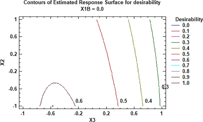
Figure 2 shows the response surface generated by the desirability function for the minimum dispersion time. The existence of an optimum for the variables X₂ and X₃ is evidenced.

Figure 2.

Surface response for the desirability function of experimental design E-2.

Table 1 shows, with greater relevance in some cases, how an important part of the substance of interest remains in the heavy phase and that in the light phase it is difficult to completely remove the aldehydes. Using the multi-objective optimization, it is possible to reach a compromise solution by following the premises of Table 3, through which it is possible to achieve acceptable levels of high-molecular-weight fatty alcohols, without sacrificing economy.

It is evident that the separation of both fractions by extraction with organic solvents is not easy, so if the properties that determine the solubility of higher fatty alcohols and aldehydes of sugarcane wax are analyzed, a better understanding of this phenomenon will be achieved.

Results Interpretation through Hansen’s Solubility Theory

For a better understanding of how Hansen’s solubility theory can contribute to the interpretation of the results obtained, the following steps have been considered:

• Estimation of the HSPs of higher fatty alcohols and aldehydes of sugarcane wax according to the Yamamoto Molecule Breaking (Y-MB) determination method and their comparison.

• Estimation of the HSPs of policosanol by considering, as experimental test, the solubility reports of the literature for policosanol and octasonol (as a majority compound of policosanol).

• Determination of the HSPs of policosanol according to the volumetric composition of its compounds.

• Effect of temperature on the affinity between solutes and the solvent/solute ratio

Table 9 reports the estimates of the Hansen solubility parameters for the various higher fatty alcohols and aldehydes of the sugarcane wax according to the Yamamoto Molecule Breaking (Y-MB) determination method.

Table 9. Hansen Solubility Parameters of Some Aldehydes and Alcohols Present in the Sugarcane Wax.

aldehydes	δD (MPa1/2)	δP (MPa1/2)	δH (MPa1/2)	molecular weight	molar vol. (cm3/mol)	Ra at 25 °C	Ra at 75 °C
tetracosanal	16.0	3.2	2.0	352.6	419.1	18.28	16.87
hexacosanal	16.0	2.8	1.9	380.69	452.0	18.50	17.09
octacosanal	15.9	2.8	1.8	408.74	485.1	18.60	17.16
triacontanal	16.0	2.5	1.7	436.8	518.0	18.79	17.38
dotriacontanal	16.0	2.0	1.5	478.88	567.9	19.15	17.75
tetratriacontanal	16.0	2.2	1.5	492.9	583.9	19.08	17.68
hexatriacontanal	15.9	2.3	1.4	521.0	617.0	19.14	17.71
Fatty Alcohols
tetracosanol	15.9	2.0	5.5	354.66	422.7	15.48	14.13
hexacosanol	15.9	1.9	5.1	382.72	455.2	15.88	14.53
heptacosanol	15.9	2.0	4.8	396.73	471.7	16.11	14.74
octacosanol	15.9	1.7	4.5	410.77	488.6	16.51	15.14
nonacosanol	16.0	1.7	4.3	424.79	504.5	16.69	15.35
triacontanol	15.9	1.7	4.2	438.81	521.2	16.78	15.41
dotriacontanol	15.9	1.5	3.6	466.87	554.6	17.41	16.03
tetratriacontanol	15.9	1.5	3.3	494.90	587.1	17.68	16.29

As can be seen, the HSPs for aldehydes and higher fatty alcohols are almost similar, except for the hydrogen bonding parameters (δ_H), which are slightly higher for alcohols, which generates a solute/solvent distance (R_a) in favor of the higher fatty alcohols. As mentioned, an increase in temperature produces a reduction in HSPs, mainly for δ_H.

Additionally, if various literature reports on the solubility of policosanol and octacosanol in organic solvents are used as the basis of an “experimental” Hansen test, as summarized in Table 10, estimates of the Policosanol HSPs of 16.06, 2.41, and 5.02 are obtained for δ_D, δ_P, and δ_H, respectively, as well as a Hansen sphere radius (R₀) of 9.6. These results were obtained with the genetic algorithm and are similar to those reported in Table 9 for higher fatty alcohols. The resulting Hansen sphere for this test is shown in Figure 3.

Table 10. Experimental Test for HSPs of Policosanol/Octacosanol Determination Based on the Solubility Criteria Reported by Several Authors.

solvent	δD (MPa1/2)	δP (MPa1/2)	δH (MPa1/2)	score	RED	molar volume (cm3/mol)	refs
1-pentanol	15.9	5.9	14	1	0.938	108.6	(34)
1-hexanol	15.9	5.8	13	1	0.811	125.2	(34)
acetone	15.5	10	7	1	0.822	73.8	(40)
dichloromethane	17.0	7.3	7.1	1	0.586	64.4	(41)
ethyl acetate	15.8	5.3	7.2	1	0.376	98.6	(40)
chloroform	17.8	3.1	5.7	1	0.400	80.5	(42)
toluene	18.0	1.4	2	1	0.510	106.6	(34)
benzene	18.4	0	2	1	0.606	89.5	(35)
heptane	15.3	0	0	1	0.525	147.0	(40)
hexane	14.9	0	0	1	0.544	131.4	(43)
water	15.5	16	42	0	3.837	18.0	(35)
ethanol	15.8	8.8	19	0	1.535	58.6	(23)a

^aConsidered not a good solvent at ambient temperature.

Figure 3.

HSP sphere for policosanol resulted from HSPiP software analyses of Table 10 data.

The mass and volumetric compositions of policosanol are illustrated in Table 11, so the estimated policosanol HSPs from the HSP values reported for each higher alcohol in Table 9 would be 15.90, 1.70, and 4.41 for δ_D, δ_P, and δ_H respectively, similar to those determined in the previous “experimental” solubility test.

Table 11. Mass and Volumetric Compositions of Policosanol Used for Policosanol HSP Estimation.

	mass conc. limits (%)
compound	minimum	maximum	mass conc. (%)	volumetric conc. (%)
tetracosanol	0.01	2.00	1.00	1.00
hexacosanol	3.00	10.00	5.03	5.03
heptacosanol	0.10	3.00	1.50	1.50
octacosanol	60.00	70.00	69.27	69.29
nonacosanol	0.10	2.00	1.00	1.00
triacontanol	10.00	15.00	12.15	12.13
dotriacontanol	5.00	10.00	7.05	7.04
tetratriacontanol	0.10	5.00	3.01	3.00

The HSPs of pure ethanol at 25 °C are 15.8, 8.8, and 19.4 for δ_D, δ_P, and δ_H, respectively, while at 75 °C the values of ethanol HSPs are 14.8, 8.6, and 17.8.

The approximation between the higher alcohol and aldehyde groups can be seen in Figure 4, where the Hansen coordinates are also represented for ethanol at 25 and 75 °C, respectively. As can be observed in Table 9, the distance R_a between ethanol and these wax compounds becomes smaller as the temperature increases, although they are not very different between the two groups, which supports the difficulty of achieving an accurate separation between alcohols and aldehydes with the use of this solvent.

Figure 4.

Planar representation of the HSPs of aldehydes, higher fatty alcohols, and ethanol at 25 and 75 °C, and the relationship between them using HSPiP software.

Calculation of ethanol–water mixtures’ HSPs increases the complexity of the analysis because the δ_H parameter of water falls dramatically with increasing temperature; moreover, water is a good plasticizer and also increases the diffusion rates.¹⁷ Fatty alcohols and aldehydes with long chains of carbon atoms behave in a similar way to polymers, and the affinity for water is manifested in the same way. For this reason, ethanol with 5 and 10% v/v of water is capable of extracting aldehydes and alcohols with increasing temperature, although the yield and composition of the extracted fraction change, as seen in Tables 1 and 6.

Furthermore, with increasing temperature, the thermodynamic factors described by Louwerse et al.⁴⁴ are manifested with greater intensity. These authors reviewed the Hansen approach to solubility parameters considering the thermodynamics of dissolution and mixing; several corrections are suggested, such as taking into account the size of the solvent and solute molecules, the destruction of the crystalline structure of the solid, as occurs in the case of the of wax melting, and the specificity of the hydrogen bonding.

If it is considered that the higher fatty alcohols and ethanol at 75 °C could be within the Hansen solubility sphere and the aldehydes are excluded, a Hansen sphere like the one illustrated in Figure 5A is reached, where aldehydes and ethanol at 25 °C are out of the sphere. Nevertheless, the aldehydes are on the limit of the sphere surface with relative energy difference values (RED = R_a/R₀) close to unity, indicating the possibility of being solubilized by hot ethanol, as it really happens.

Figure 5.

(A) Possible Hansen solubility sphere for higher fatty alcohols and ethanol at 75 °C and 25 °C. (B) Hansen solubility sphere considering donor/acceptor properties and the molar volume of solutes and solvents: (a) higher fatty alcohols and aldehydes with high molar volume, (b) ethanol at 75 °C, (c) ethanol at 25 °C.

However, if the donor/acceptor properties and molar volume of solutes and solvents are considered, the solubility sphere will change as illustrated in Figure 5B, where the aldehydes, classified as not soluble in hot ethanol, fall inside the Hansen solubility sphere. Because of that, a fraction of the aldehydes are also solubilized by hot ethanol; moreover, ethanol has a small molar volume, which increases its diffusion in wax fraction to extract the solutes: higher fatty alcohols, but also some aldehydes.

The temperature effect and other thermodynamic considerations explain why ethanol at low temperature is a good solvent for the wax–oil fraction¹⁶ and is considered a bad solvent for the wax fraction evaluated at 25 °C.²³ On increasing the temperature, it becomes a good solvent.

Conclusions

The novelty of the work, in addition to the separation of fatty alcohols and aldehydes with the use of ethanol and the optimization of the sugarcane wax fractionation conditions to adapt it to the quality of the raw material for the production of policosanol, consists in the contribution to the understanding of this result through Hansen’s solubility theory. It explains how a solvent reported as not feasible for the extraction of the wax fraction is suitable for the fractionation of sugarcane wax under certain temperature and operating conditions. However, it is also evident that due to the affinity between alcohols and fatty aldehydes, the precise extraction of one of them is extremely difficult without the presence of certain amounts of the other.

In fact, the study demonstrated the possibility to obtain a sugarcane wax fraction rich in higher fatty alcohols for policosanol production with the use of ethanol as a solvent. It is verified that it is possible to achieve the extraction of higher fatty alcohols with a low concentration of aldehydes or impurities and to keep a compromise between quality and cost with the use of ethanol–water mixtures between 90–95% v/v, and low dispersion times of the wax in the solvent and solvent/wax ratios of 12–14:1 v/w. The analysis of Hansen solubility parameters and their relationships with temperature is a useful tool to understand the complexity involved in the separation between the higher fatty alcohols and aldehydes present in sugarcane wax, as well as the difficulty of their fractionation by means of solvent extraction.

Glossary

Abbreviations

GC

gas chromatography

HSPs

Hansen solubility parameters

Author Contributions

The manuscript was written through the contributions of all authors. M.D.R. and E.H.R. designed the research and conducted the experiments with R.V.M. and K.P.C. V.G.C. and R.V.M. did the V.G.C. analysis. L.Z.C. did the statistical analysis with M.D.R. and E.H.R. All authors have given approval to the final version of the manuscript.

The Cuban Research Institute for Sugarcane Derivatives (ICIDCA) and National Center for Scientific Research (CNIC) supported the research.

The authors declare no competing financial interest.

References

- Mohan S.; Chithra L.; Nageswari R.; Manimozhi Selvi V.; Mathialagan M. Sugarcane Wax - A Par Excellent by-Product of Sugar Industry – A Review. Agric. Rev. 2021, 42, 315–321. 10.18805/ag.R-2055. [DOI] [Google Scholar]
- Avequin M. de wasachtige Matter of Sugarcane. Ann. Chim. Phys. 1840, 75, 218–222. [Google Scholar]
- Ray S. C.Studies of Conversion of Crude Waste Extracted from Sugar Cane Pressmud in Industrial Quality Wax, Ph.D. Thesis, Faculty of Engineering & Technology, Swamiramanand Teerth Marathwada University, 2003. [Google Scholar]
- Lachos-Perez D.; Barrales F. M.; Martinez J.; Maciel Filho R. Supercritical CO2 Extraction of Lipophilic Molecules from Sugarcane Straw. Chem. Eng. Trans. 2020, 80, 313–318. 10.3303/CET2080053. [DOI] [Google Scholar]
- García A.; García M. A.; Ribas M.; Brown A. Recuperación de cera de cutícula de caña de azúcar mediante separación mecánica y extracción con solventes. Grasas Aceites 2003, 54, 169–174. 10.3989/gya.2003.v54.i2.261. [DOI] [Google Scholar]
- Bhosale P. R.; ChondeSonal G.; Raut P. D. Studies on extraction of sugarcane wax from press mud of sugar factories from kolhapur district Maharashtra. J. Environ. Res. Dev. 2012, 6, 715–720. [Google Scholar]
- Swenson O. J.Method of Extracting Wax from Cachaza. U.S. Patent US2508002A, 1947.
- Rhodes F. H.; Swenson O. J. U.S. Patent US24228813A, 1947.
- Lake A. W.Recovery of Sugarcane Wax. U.S. Patent US3931258A, 1973.
- Balch T. R.Hard Waxes and Fatty Products Derived from Crude Sugar Cane Waxes. U.S. Patent US2381420, 1942.
- Díaz M.; Hernández E. Composición de la cera de caña de azúcar y el empleo de solventes para su extracción y fraccionamiento. Enfoque orientado a su aplicación. ICIDCA sobre los derivados de la caña de azúcar 2020, 54, 13–22. [Google Scholar]
- Attard T. M.; McElroy C. R.; Rezende C. A.; Polikarpov I.; Clark J. H.; Hunt A. J. Sugarcane waste as a valuable source of lipophilic molecules. Ind. Crops Prod. 2015, 76, 95–103. 10.1016/j.indcrop.2015.05.077. [DOI] [Google Scholar]
- Inarkar M. B.; Lele S. S. Extraction and Characterization of Sugarcane Peel Wax. ISRN Agron. 2012, 2012, 340158 10.5402/2012/340158. [DOI] [Google Scholar]
- Asikin Y.Waxes, policosanols and aldehydes in sugarcane (saccharum officinarum l.) and okinawan brown sugar (kokuto), Bogor Agricultural University, Master of Science Thesis, Department of Food Science and Technology, 2008. [Google Scholar]
- Martínez R.; Castro I.; Oliveros M. Characterization of Products from Sugar Cane Mud. Rev. Soc. Quím. Méx. 2002, 46, 64–66. [Google Scholar]
- Hernández E.; Díaz M.; Pérez K. Determination of Hansen Solubility Parameters for sugarcane oil. Use of ethanol in sugarcane wax refining. Grasas Aceites 2021, 72, e408 10.3989/gya.0326201. [DOI] [Google Scholar]
- Hansen C. M.Hansen Solubility Parameters: A User’s Handbook, 2nd ed.; CRC: Boca Ratón, 2007; pp 1–26. [Google Scholar]
- Taylor T. I.; Larson L.; Johnson W. Miscibility of Alcohol and Oils. Ind. Eng. Chem. 1936, 28, 616–618. 10.1021/ie50317a030. [DOI] [Google Scholar]
- Freitas S. P.; Lago R. C. A. Equilibrium Data for the Extraction of Coffee and Sunflower Oils with Ethanol. Braz. J. Food Technol. 2007, 10, 220–224. [Google Scholar]
- Da Silva C. A. S.; Sanaiotti G.; Lanza M.; Follegatti-Romero L. A.; Meirelles A. J. A.; Batista E. A. C. Mutual Solubility for Systems Composed of Vegetable Oil + Ethanol + Water at Different Temperatures. J. Chem. Eng. Data 2010, 55, 440–447. 10.1021/je900409p. [DOI] [Google Scholar]
- Da Costa Rodrigues C. E.; Oliveira R. Response surface methodology applied to the analysis of rice bran oil extraction process with ethanol. Int. J. Food Sci. Technol. 2010, 45, 813–820. 10.1111/j.1365-2621.2010.02202.x. [DOI] [Google Scholar]
- Shariati A.; Azaribeni A.; Hajighahramanzadeh P.; Loghmani Z. Liquid Liquid Equilibria of Systems Containing sunflower Oil, Ethanol and Water. APCBEE Proc. 2013, 5, 486–490. 10.1016/j.apcbee.2013.05.082. [DOI] [Google Scholar]
- Hernández E.; Díaz M. Determination of Hansen Solubility Parameters of refined sugarcane wax. Chem. Pap. 2021, 75, 5313–5322. 10.1007/s11696-021-01717-5. [DOI] [Google Scholar]
- del Pillar Sánchez-Camargo A.; Bueno M.; Ballesteros-Vivas D.; Parada-Alfonso F.; Cifuentes A.; Ibáñez E. Hansen Solubility Parameters for Selection of Green Extraction Solvents. TrAC, Trends Anal. Chem. 2019, 118, 227–237. 10.1016/j.trac.2019.05.046. [DOI] [Google Scholar]
- Sicaire A. G.; Vian M.; Fine F.; Joffre F.; Carré P.; Tostain S.; Chemat F. Alternative Bio-Based Solvents for Extraction of Fat and Oils, Solubility Prediction, Global Yield, Extraction Kinetics, Chemical Composition and Cost of Manufacturing. Int. J. Mol. Sci. 2015, 16, 8430–8453. 10.3390/ijms16048430. [DOI] [PMC free article] [PubMed] [Google Scholar]
- Dejoye Tanzi C.; Vain M. A.; Ginies C.; Elmaataoui M.; Chemat F. Terpenes as Green Solvents for Extraction of Oil from Microalgae. Molecules 2012, 17, 8196–8205. 10.3390/molecules17078196. [DOI] [PMC free article] [PubMed] [Google Scholar]
- Araújo de Oliveira R. M.Avaliação de terpenos como solventes no processo de extração da cera de cana-de-açúcar, Dissertação de Mestrado defendida e aprovada dia 30 de julho de, Campinas, Brasil, 2018.
- Holser R. A.; Akin D. E. Extraction of lipids from flax processing waste using hot ethanol. Ind. Crops Prod. 2008, 27, 236–240. 10.1016/j.indcrop.2007.09.002. [DOI] [Google Scholar]
- Holser R. A. Temperature-dependent solubility of wax compounds in ethanol. Eur. J. Lipid Sci. Technol. 2009, 111, 1049–1052. 10.1002/ejlt.200900068. [DOI] [Google Scholar]
- Myung K.; Parobek A. P.; Godbey J. A.; Bowling A. J.; Pence H. E. Interaction of Organic Solvents with the Epicuticular Wax Layer of Wheat Leaves. J. Agric. Food Chem. 2013, 61, 8737–8742. 10.1021/jf402846k. [DOI] [PubMed] [Google Scholar]
- Inès S.; Ben Marzoug I.; Sakli F. Effect of solvent extraction on Tunisian esparto wax composition. Alger. J. Nat. Prod. 2016, 4, 308–315. [Google Scholar]
- Chakhathanbordee R.; Khotavivattana S.; Sriroth K. Development of sugarcane wax extraction methods from sugarcane filter cake for value creation. Res. Dev. J. Sci. Technol. 2016, 11, 95–106. [Google Scholar]
- Lide D. R., Ed.; CRC Handbook of Chemistry and Physics, Internet Version Taylor and Francis: Boca Raton, FL, 2006. http://www.hbcpnetbase.com. [Google Scholar]
- Cuevas M. S.; Crevelin E. J.; de Moraes L. A.; Oliveira A. L.; Rodrigues C. E.; Meirelles A. J. Solubility of commercial octacosanol in organic solvents and their correlation by thermodynamic models at different temperatures. J. Chem. Thermodyn. 2017, 110, 186–192. 10.1016/j.jct.2017.02.025. [DOI] [Google Scholar]
- Ivy Fine Chemical Coporation Octacosanol data sheet, http://www.Ivychem.com.
- Statpoint, Inc. Statgraphics Centurion Software XV, version 15.2.05, 2007.
- Marrero-Delange D.; González-Canavaciolo V. L.; Sierra-Pérez R.; Velásquez-G C. Validación de un nuevo método analítico por CG con columna capilar para la determinación de alcoholes de alto peso molecular en policosanol ingrediente active. Rev. Colomb. Cienc. Quím. Farm. 2008, 37, 62–68. [Google Scholar]
- Lamberton J. A. The long-chain aldehydes of sugar-cane wax. Aust. J. Chem. 1965, 18, 911–913. 10.1071/CH9650911. [DOI] [Google Scholar]
- Abbott S.; Yamamoto H.. HSPiP Software, 5th edition, 2015.
- Srisaipet A.; Luangpitak P.; Potisen P. The Policosanol Extraction and Composition Characterization from Wheat Straw By-Product of Thai Wheat Varieties. Int. J. Food Eng. 2019, 5, 99–103. 10.18178/ijfe.5.2.99-103. [DOI] [Google Scholar]
- Srisaipet A.; Keawprom P. Extraction And Characterization Of Policosanol From Wheat Germ. Int. J. Eng. Technol. 2018, 7, 1478–1482. [Google Scholar]
- Asikin Y.; Chinen T.; Takara K.; et al. Determination of Long-chain Alcohol and Aldehyde Contents in the Non-Centrifuged Cane Sugar Kokuto. Food Sci. Technol. Res. 2008, 14, 583–588. 10.3136/fstr.14.583. [DOI] [Google Scholar]
- Singh A. K.; Chandra A.; Kandpal J. B. Octacosanol extraction, synthesis method and sources: a review. Carpathian J. Food Sci. Technol. 2020, 12, 27–41. 10.34302/crpjfst/2020.12.5.2. [DOI] [Google Scholar]
- Louwerse M. J.; Maldonado A.; Rousseau S.; Moreau-Masselon C.; Roux B.; Rothenberg G. Revisiting Hansen Solubility Parameters by Including Thermodynamics. ChemPhysChem 2017, 18, 2999–3006. 10.1002/cphc.201700408. [DOI] [PMC free article] [PubMed] [Google Scholar]