Visualization and Quantification of Geometric Diversity in Metal–Organic Frameworks

Abstract

With ever-growing numbers of metal–organic framework (MOF) materials being reported, new computational approaches are required for a quantitative understanding of structure–property correlations in MOFs. Here, we show how structural coarse-graining and embedding (“unsupervised learning”) schemes can together give new insights into the geometric diversity of MOF structures. Based on a curated data set of 1262 reported experimental structures, we automatically generate coarse-grained and rescaled representations which we couple to a kernel-based similarity metric and to widely used embedding schemes. This approach allows us to visualize the breadth of geometric diversity within individual topologies and to quantify the distributions of local and global similarities across the structural space of MOFs. The methodology is implemented in an openly available Python package and is expected to be useful in future high-throughput studies.

Introduction

A cornucopia of experimentally determined crystal structures is described in continually expanding databases.^1,2 These databases are now reaching sufficient sizes to provide an opportunity for extracting structure–property relationships based on data mining and machine learning (ML), in principle.³⁻⁵ Establishing these relationships, however, is a nontrivial task because there are multiple ways by which crystal structures can be represented, compared, and analyzed. This challenge is particularly acute for metal–organic frameworks (MOFs) where the diversity of both the metal centers (“nodes”) and the organic linkers gives rise to considerable structural complexity.⁶⁻⁹

One of the ways in which MOFs are commonly described is in terms of their topology; that is, the connectivity between nodes and linkers. Topological analysis routines are well-established and are implemented in automated computer packages, such as ToposPro(10) and Systre,¹¹ and have been found to be useful predictors for a number of material properties. For example, by considering the deformability afforded by a given topology (i.e., the ability of a framework to distort geometrically without disrupting the net connectivity), one may predict the rigidness of a framework,¹² the tendency to interpenetrate,¹³ and elastic properties.^14,15 Ultimately, by exploiting knowledge of how a given choice of the node and linker will give rise to a particular topology, one can hope to design new MOFs.¹⁶⁻¹⁸

However, two MOFs with the same topology may have very different network geometries. By the latter term, we mean the spatial arrangement of local atomic environments in a MOF, including variations in bond lengths, angles, and longer-range ordering—all of which may affect material properties. For example, positive and negative thermal expansion can be switched in MOFs of a given topology simply by varying their geometry.¹⁹ By their very nature, however, each of the established geometric descriptors will cover only individual aspects of the structure; two MOFs with similar metal–linker distances might have different porosities, for example.

Atom-density-based representations offer an alternative means of quantifying the geometric similarity of crystal structures.²⁰⁻²² One class of such metrics originated in the field of ML for physics and chemistry applications, where the development of structural descriptors for the atomistic structure is one of the central research tasks.²³⁻²⁷ In particular, the smooth overlap of atomic positions (SOAP) descriptor was developed initially in the context of fitting machine-learned interatomic potentials.²⁸ Subsequently, it was shown how similarity kernels based on the SOAP formalism may be used to analyze the structural similarity for molecular and bulk periodic structures.²⁹

By coupling to ML techniques such as dimensionality reduction and data clustering, one can begin to navigate complex configuration spaces³⁰⁻³² and search for underlying structure–property relationships.³³⁻³⁸ We have recently demonstrated that a combination of coarse-graining, rescaling, and SOAP analysis enables the geometric comparison between very different classes of materials, exemplified using a database of the AB₂ hybrid and inorganic networks.³⁹ Other studies have emphasized the usefulness of unsupervised³¹ and supervised⁵ ML for MOFs, and very recently, local coordination environments were used as features for predicting oxidation states in these materials.⁴⁰

Here, with a view to facilitate further quantitative studies of the geometric structure and structure–property relationships in MOFs, we describe a generalized coarse-graining approach for such purposes and its implementation in an openly available Python package, which we call CHIC (“Coarse graining of Hybrid and Inorganic Crystals”)—expanding widely on the initial work in ref (39). Using a curated test set of four-connected AB₂ coordination networks, we validate structure outputs of our implementation using the well-established ToposPro topology analysis and then discuss examples of structural and chemical analysis that are enabled by our approach.

Methodology

The computational methodology can be separated into two stages: structure processing and structure analysis (Figure 1). Each stage will be discussed in turn in the following subsections. References to functions contained within the code will be highlighted in typewriter typeface throughout. We summarize the main aspects here; a separate tutorial and a practical demonstration of using the code can be found in an interactive Jupyter notebook (as detailed in the Data and Code Availability section).

Figure 1.

Methodology for processing and analyzing MOF structure data sets using a cg-SOAP-based approach (cf. ref (39)). Left: structures from the experimental literature may first need to be “cleaned-up” for analysis. Here, as in ref (39), ZIF-8 is used as an example: the H-disorder is resolved using average positions of half-occupancy sites, and guest atoms in the pores are removed. The structure is then reduced to its constituent building blocks, viz., 12 Zn²⁺ A sites (purple) and 24 methyl imidazolate B sites; the latter sites are coarse-grained using connectivity graphs (here, identifying the five-membered imidazolate rings as the B-site centers, yellow). Right: the SOAP kernel is used to determine the similarity between all coarse-grained and rescaled structures in the database, and the result is visualized using dimensionality reduction. The resultant 2-D structure map (sketched here in a purely schematic way) may then be interpreted by correlating the locations of data points with structural and physical properties.

Structure Processing

The main structure-processing routines of our implementation are handled by a Python class called Structure. It uses Pymatgen(41) to parse and store information in the crystallographic information file (CIF) format. All subsequent structure-processing tasks are then callable as attributes of the Structure class as follows.

sort_sites()

Initially, the atomic species are classified into two categories: A (metal) sites and “other” sites. In the absence of user-specified categories, elements are sorted according to the IUPAC International Chemical Identifier classification:⁴² metals are assigned to A sites and nonmetals are assigned to “other”. In the present work, we focus on the geometric structure of the underlying nets (as opposed to also considering the energetic stability provided by guest ions and molecules), and therefore, we remove nonframework species. Alkali and alkaline-earth metals (excluding Li and Be) are often nonframework atoms and are therefore removed during the species sorting algorithm (and ultimately from the final coarse-grained structure). B, Si, and P are also sorted on a case-by-case basis because there are many instances in which they behave as either A or “other” sites (e.g., boron is an A site in boron imidazolate frameworks⁴³ but a nonframework-site atom when a part of a BF₄^– anion). Therefore, if the element is bound to O or N—indicative of Lewis-acidic-type behavior—it is assigned as an A site. It should be noted that such modifications to the sorting algorithm are made based on the chemical nature of the data set being studied and serve primarily to minimize the requirement for user input during the coarse-graining procedure. The modifications may therefore be amended or removed in future work, without affecting the conclusions herein.

repair_disorder()

Site disorder occurs frequently in MOFs, and it is commonly modeled crystallographically using split sites with partial occupancies.⁴⁴ To enable structure-processing tasks that require discrete atomic positions, partially occupied (or disordered) sites are simplified using three algorithms, callable with the Structure.repair_disorder() method. First, atoms of the same species found within a given distance range (0–0.7 Å by default) are replaced by an atom of the same type, situated on the average of their positions. The remaining two routines deal with delocalized electron density associated with guest species within framework pores, which is often modeled by clusters of (fictitious) oxygen atoms. These clusters are removed by identifying either oxygen atoms that only have oxygen nearest neighbors or oxygen atoms that have no neighbors at all within a set cutoff radius. Not all disorder needs to be resolved for the general coarse-graining procedure to work; the minimum requirement is that individual molecules (e.g., organic ligands) do not overlap. However, unresolved disorder may affect the placement of the discrete place-holder atoms (e.g., by skewing the centroid of a given molecule).

reduce()

Each unique building block fragment, or ligand, is then identified by a “nearest-neighbor crawl” algorithm by calling the Structure.reduce() method. The default neighboring-site routine used is CrystalNN,⁴⁵ as implemented in Pymatgen.⁴¹ In short, CrystalNN uses Voronoi decomposition to assign weights to an initial list of neighbors within a hard cutoff radius and then normalizes and assigns probabilities to each unique weighting according to a smooth cutoff function. With this definition, a building block fragment list is initialized with a given atom from a given building block type, and if another atom is both a nearest-neighbor and of the same building block type, it is added to the list. These neighbors are then searched for their respective nearest-neighbors, and the process is iterated (thereby “crawling” round the ligand) until the list size converges. Once converged, the atomic species, positions, and connectivity (in the form of a connectivity graph) of the fragment are stored as a buildingUnit class instance and appended to the Structure.units class attribute. The algorithm repeats until all atoms have been classified.

coarse_grain()

To coarse-grain the building blocks, a discrete bonding center must first be defined. There is seldom a unique choice for this. The simplest definition is to take the geometric centroid of all of the atomic positions in the building unit (i.e., not weighted by the atomic masses). This parallels the methodology used in both crystal net determination (often referred to as “equilibrium” or “barycentric” placement)¹¹ and coarse-grained molecular dynamic simulations⁴⁶ and is the definition used in the present work. The buildingUnit class stores the connectivity of a given building unit as a graph object using the NetworkX package,⁴⁷ thereby enabling alternative bonding centers to be defined. These alternative definitions are not used in the present work but are explored in a Jupyter notebook that is provided with the code (see the Data and Code Availability section).

The building-unit connectivity is defined as the number of nearest-neighbor atoms of a different site type which are connected to a given fragment. All fragments with connectivity >1 (thereby distinguishing nonframework species, such as solvents, from the B sites) are coarse-grained by placing a dummy atom at the chosen bonding center and removing all other atoms. Finally, all atoms of a given building-block type are assigned to the same atomic species. The processed structures can then be output in the CIF format.

Structure Analysis

Studying large, complex data sets requires generalized analysis routines. At the core of our analysis class, StructureMap, structures are compared using SOAP²⁸ which we apply to coarse-grained structural models (indicated by “cg-SOAP”).³⁹ Using dimensionality reduction algorithms, configurations can be visualized and the relationships between them then analyzed.

cg-SOAP

The SOAP kernel measures the similarity of pairs of atomic environments.^28,29,32 Formally, for each atom, α, an atomic density, ρ_α(r), is constructed with a sum of Gaussians of broadness σ, centered on each neighbor, β, of α (and on α itself):

1

where f_cut denotes a cutoff function. The SOAP kernel is then defined as the overlap integral of any two neighbor densities, integrated over all three-dimensional rotations R̂,²⁸

2

where the exponent is typically set to n > 1 to retain angular information.²⁹ In practice, it is computationally more efficient to expand the atomic density in a set of orthogonal radial basis functions and spherical harmonics up to a given n_max and l_max. The resulting combination coefficients on their own do not yet ensure rotational invariance (because all spherical harmonics with l > 0 depend on the angular orientation) and are therefore collected into a power spectrum vector. The SOAP kernel may then be calculated by taking the normalized dot product of the two power spectrum vectors associated with each atomic environment, raised to an exponent ζ which serves to accentuate the distinction between the two environments.²⁸

As shown in ref (48) for elemental structures and in ref (39) for a range of inorganic and hybrid materials, geometric similarity may be assessed using SOAP for uniformly rescaled structures, enabling direct comparison irrespective of characteristic A–B distances. We have implemented two scaling approaches: either scaling to a uniform minimumr(A–B) distance or scaling to a uniform averager(A–B) distance.

To extend the similarity measure beyond comparing individual atomic environments, similarities between pairs of atoms in each of the crystal structures are calculated:

3

where α (β) runs over all atomic sites, , in the unit cell of structure i (j), respectively. Variations of this method are also implemented where the atomic sites considered are restricted to a given site type (e.g., A sites), thereby shifting the focus of the similarity analysis toward those particular sites. (In this case, information regarding the other site types is still implicitly encoded through the neighbor densities.)

Dimensionality Reduction and Visualization

To interpret (cg-)SOAP analysis results, the data set is often visualized as a two-dimensional projection.^29,32,39 A large number of algorithms are available to carry out this projection (or “embedding”), and a central aspect of the present work will be to compare different widely used embedding schemes. Our implementation stores the similarity of all structures with one another in the form of a symmetric similarity matrix, K, which we construct using the per-cell averaged similarity (eq 3), viz., . The corresponding geometric distance matrix, D, may also be defined with elements

4

to satisfy the triangle inequality.²⁹ We currently provide interfaces to the following dimensionality reduction algorithms implemented in external code packages: multidimensional scaling (MDS),⁴⁹ t-distributed stochastic neighbor embedding (t-SNE),⁵⁰ and the uniform manifold approximation and projection (UMAP).⁵¹

Bonding and Properties

During the reduction of MOF structures to their coarse-grained representations, a dictionary of bonds between building units is stored, as recently defined in the IUCr topology dictionary (topoCIF). This enables the CIF output to contain the requisite information to readily construct the underlying net,^52,53 that is, the net of building units, and to calculate its topological descriptors (e.g., using ToposPro). It also enables the calculation of local-environment properties, including bond lengths, angles, and order parameters. We use a module, referred to as bonding, to extract this geometric information and calculate Chau–Hardwick tetrahedral order parameters and Steinhardt bond order parameters.⁵⁴⁻⁵⁶ This module might also be extended for other custom analyses.

Two global structure properties are also included in the routine structure analysis. The first is A-site density, an important material descriptor when considering the potential void space present in a framework. The second property is the A-site SOAP heterogeneity introduced in previous work,³⁹ which measures the diversity of the A-site environments in a given structure. A value of zero means that all A-site environments are geometrically equivalent (up to the SOAP cutoff radius); a higher value indicates greater diversity. It is calculated as

5

where P is the set of (unordered) pairs of distinct A-site environments in the structure, is the number of A-site atoms in the structure, and k is the SOAP similarity kernel defined in eq 2.

Database Details

The data set curated for this work expands upon the AB₂ study reported in ref (39), now focusing on analyzing the diversity in the wider set of AB₂ MOFs with two-connected ligands. Restricting the study to a single coordination formula and ligand connectivity enables careful validation of the reported coarse-graining methods and a thorough examination of the results; in particular, being able to relate trends in our configuration space to local geometric properties of individual structures serves as a useful tool for understanding what information is captured in the cg-SOAP approach.

Primary data were selected from the sample that was prepared for ref (13), filtering for all structures in which the coordination formula was AB₂ and the ligand (B) was two-connected. The sample contained 1160 crystal structures, to which 102 structures from the CSD 5.42 update 1 (Feb 2021) were added. A complete list of the 1262 crystal structures and their topological descriptors is provided in Supporting Information (see the file CF_A_B2_1262.xlsx). The “experimental literature” to be processed was exported as CIFs from the CSD using the 1262 entry refcodes and processed unchanged.

Results and Discussion

Visualizing Geometric Diversity

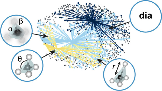
We begin by visualizing the geometric diversity in the AB₂ MOF data set, here embedding cg-SOAP similarities for all (uniformly scaled) structures in two dimensions. Dimensionality reduction is an unsupervised ML task, aiming to extract information from unlabeled data sets, for example, by clustering the data into groups. We start by visualizing the data set using one of the simplest algorithms, MDS (as used in ref (39)), in Figure 2. The structure map carries the intuitive interpretation that structures that are similar appear close together and structures that are dissimilar are further apart. In the context of MOFs, structures are generally reported with their topological identifier which uniquely identifies the underlying net. We highlight the distribution of the three most commonly occurring topologies in the data set—the diamond-like dia net (189 structures), the sodalite-like sod net (136 structures), and the fourfold interpenetrated 4#dia net (116 structures)—to investigate the degree to which topological variation is represented in the cg-SOAP representation. Strikingly, all three topological families have structures dispersed over the map, with the dia topology being most widely distributed among the three (light blue). There are regions of overlapping points, particularly for dia and sod in the lower part of Figure 2, indicating that topologically dissimilar MOFs might in fact show similarities in terms of their geometric structure.

Figure 2.

Geometric diversity within isoreticular groups of AB₂ MOFs. The graph shows a two-dimensional visualization of the cg-SOAP-based structural distances using an MDS embedding: generally, the closer the two points are, the more similar their coarse-grained and rescaled geometric structures are. The distribution of the three most commonly occurring topologies within our data set (dia, sod, and fourfold-interpenetrated dia, denoted as 4#dia) is emphasized by lines that originate from the respective centroid. Data set entries with different topologies than the three aforementioned ones are all represented by gray points.

We quantify the relative distributions of each topology in the map based on how far, on average, the structures of that group are from their respective centroid. These relative distributions are 0.771, 0.386, and 0.441 for dia, sod, and 4#dia, respectively. For ease of comparison, we normalize the relative distributions such that the value for dia is unity (Table 1).

Table 1. Characteristics of the Ten Most Commonly Occurring Topologies in the Data Set.

		geometric densitya	relative distribution
topology	occurrences	(mean ± SD)	MDS	t-SNE	UMAP
dia	189	125 ± 56	1 (reference)
sod	136	80 ± 26	0.50	0.45	0.60
4#dia	116	261 ± 77	0.57	0.47	0.44
5#dia	95	271 ± 87	0.67	0.47	0.50
3#dia	88	206 ± 76	0.71	0.48	0.45
2#dia	79	182 ± 82	0.91	0.76	0.55
cds	41	221 ± 87	0.81	0.54	0.44
qzd	38	156 ± 15	0.12	0.18	0.26
6#dia	36	336 ± 137	0.74	0.55	0.47
3#dmp	33	292 ± 49	0.38	0.23	0.31

^aThe geometric density is here defined as n(A) × 1000/V_scaled, where n(A) is the number of A sites in the unit cell and V_scaled is the volume of the scaled unit cell.

We see that dia networks can be formed with a much larger variety of geometries compared to sod; this is in accordance with the conclusions derived from an analysis of the natural tiles (cages).¹³ This reflects a larger deformability of diamondoid structures and adaptability to building blocks with geometries spanning a wide range of volumes, lengths, and angles. This feature promotes the dominance of the dia topology in coordination networks.¹³ The folding of the dia networks into interpenetrating arrays, however, significantly restricts the diversity of acceptable network geometries.

Cluster analysis can assist the interpretation of complex data sets by grouping data and identifying representative examples, from which patterns can more readily be identified. Affinity propagation is a clustering algorithm that views each data point as a node in a network and recursively minimizes the edge weights between nodes; the magnitude of each edge at a given time reflects the current affinity the point has for selecting the second point as its “examplar”.⁵⁷Figure 3a shows the dia structures (light blue data points in Figure 2) now divided into four clusters, with the exemplar coarse-grained structures visualized. From these clusters, we investigate the distribution of structural properties in different regions of the map in order to appreciate the geometric diversity available within the dia topology. In the context of MOFs, low metal densities are the simplest indication for the presence of void space: an important feature for catalytic applications. We define the geometric density as the (unitless) density of the structures that have been coarse-grained and scaled (to unity minimum r(A–B) bond length). The geometric density is related to the experimental metal density by the characteristic framework bond length. We plot the distribution of the geometric density, average angular component of the Chau–Hardwick order parameter, S_g (a value of zero corresponds to ideal tetrahedral bond angles; a value of unity would correspond to the extreme case where all four bonds are superimposed), and the average A−B−A angle in Figure 3b–d, respectively.

Figure 3.

Geometric diversity within MOFs of dia topology. (a) From the data set characterized in Figure 2, we isolate the dia entries and analyze their distribution using a clustering algorithm, viz., affinity propagation.⁵⁷ For each cluster, the algorithm selects an “examplar” datapoint, and the corresponding coarse-grained structures and their CSD refcodes are shown. Distributions of local properties for each cluster are presented on the right-hand side: (b) the geometric density, (c) the average angular component of the Chau–Hardwick order parameter, S_g, and (d) the average A−B−A angle. Throughout this paper, box plots are drawn such that boxes range from the 25th to the 75th percentile, with the median indicated by a horizontal line; whiskers span ±1.5 times the interquartile range, and points outside this range are plotted with circle markers.

Figure 3b shows the distribution of geometric density for each cluster. There is a relatively clear separation between each group, with cluster 2 (orange) containing notably more dense frameworks. It is interesting to note that clusters 2 and 4, which have higher average geometric density, also seem to have a broader distribution across the MDS map, relative to the narrow distributions of clusters 1 and 3. This could, in part, be explained by the relatively high deviation away from ideal tetrahedral bond angles about the A sites, as evident from the plot of the angular Chau-Hardwick tetrahedral order parameter, S_g (Figure 3c). Figure 3d shows the distribution of the average A−B−A bond angle; again, clusters 2 and 4 demonstrate broad distributions with lower average values.

We extend the analysis of the dia subset of structures using parameters extracted using ToposPro;⁵³ in particular, the tile average distortion¹³ supports the results illustrated in Figure 3. Clusters with higher average geometric density have larger distortions in the tetrahedral coordination of the A sites, corresponding to a collapse of the tiles. Conversely, the most porous structures have A site coordination environments closer to an ideal tetrahedron and the largest proportion of tiles close to the adamantane tile of the ideal dia net. Analogously, structures with A−B−A angles less than 150° also correspond to denser structures due to the collapse of tiles.

Figure 2 emphasizes that a single topological classification may give rise to a geometrically diverse set of structures; that is to say, one cannot necessarily predict the geometric features of a structure from its topological label alone. From Figure 2, we therefore infer that the study of the latent geometric configuration space may provide insights into a different set of material properties (e.g., bulk modulus) compared to those which are accounted for by the topology (e.g., porosity¹³).

Embedding Schemes

The universal aim of dimensionality reduction algorithms is to capture a meaningful structure in high-dimensional data when embedded into low dimensions. However, it is imperative to consider the algorithm methodology when interpreting the structure map. To illustrate this point, we have visualized our data set with three dimensionality reduction algorithms; namely, MDS,⁴⁹ t-SNE,⁵⁰ and UMAP⁵¹ (Figure 4). Our principal aim is to demonstrate that the interpretation of our cg-SOAP representations is invariant to the specific embedding scheme chosen; indeed, there are other algorithms available (e.g., kernel principal component analysis⁵⁸ and variants thereof⁵⁹) that are not considered in this study but could be used in future work for alternative and/or complementary interpretations of the configuration space. In order to understand how each representation differs from one another, we color-code the map by the geometric density (Figure 4a) and by the distributions of dia, sod, and 4#dia topologies (Figure 4b, cf. Figure 2), and compare side-by-side how these properties are represented in the results of different embedding schemes.

Figure 4.

Visualizing geometric diversity in MOFs using different embedding schemes. The plots compare the results of multidimensional scaling (MDS,⁴⁹left), t-distributed stochastic neighbor embedding (t-SNE,⁵⁰center), and uniform manifold approximation and projection (UMAP,⁵¹right). For each embedding scheme, we show two-dimensional structure maps characterizing the coarse-grained and scaled AB₂ MOF data set, colored (a) by geometric density, and (b) with the distribution of the three most commonly occurring topologies in the data set, dia, sod, and 4#dia, highlighting the respective centroids as in Figure 2.

All three embeddings demonstrate a strong correlation of the distribution of points with geometric density and qualitatively similar trends in the relative distributions of topologies within each structure map (Table 1). The detail, however, varies. MDS leads to a distinct region in the center of the map where no structures are found. This perhaps suggests that this algorithm, which seeks to minimize a relatively simple loss function, is reaching its limits of usefulness for the size and complexity of the data set considered here.

The “island-like” features in both the t-SNE and UMAP representations—or more specifically, the absence of islands in the MDS representation—further emphasize this point. The most prominent island (right-hand side of the t-SNE map and upper-right of the UMAP map) is a family of qzd MOFs, with the smallest relative distribution, among the 10 most commonly occurring topologies in the data set, for MDS and t-SNE (Table 1). Manual inspection of the structures reveals a high frequency of similar CCDC reference codes (refcodes). The refcode system is designed to group together structures into families, such as the same compound having been crystallized and characterized under different conditions, or polymorphs of the same compound. There are two families of refcodes within the qzd MOF cluster: LIWDEB (13 occurrences) and UKUVOL (21 occurrences).^60,61 All of these structures are one of two isomers of [{Cu(succinate) (4,4′-bipyridine)}_n], isolated under different experimental conditions, and thus could be considered duplicates. The high geometric similarity between duplicates relative to the similarity between other structures in the data set skews the representation toward creating an isolated cluster.

Islands and Duplicates

The occurrence of “islands” of structures, separated out near the edge of the t-SNE and UMAP representations, requires a more subtle interpretation. For example, one of the islands to the left of the UMAP map corresponds to structures with zni and coi topologies (α and β polymorphs of Zn(Im)₂, respectively), predominantly classified within the IMIDZB refcode family. “Duplicates” cannot necessarily be identified as those with a common refcode; however, cg-SOAP screening can help automate this procedure. To illustrate this point, we isolate the IMIDZB family of structures from the database, create a structure map using t-SNE (because this algorithm generally achieves clearer clustering of data into distinct regions, albeit at the cost of meaningful intercluster distances), and analyze the representation using affinity propagation, as shown in Figure 5.

Figure 5.

Using cg-SOAP analysis to identify relationships between individual CSD entries with a single refcode. The example case here is given by the polymorphs of Zn(Im)₂, with CSD refcodes IMIDZB, suffixed with numbers representing a running index. The geometric diversity within the IMIDZB refcode family is visualized using t-SNE embedding and a cluster analysis by affinity propagation. The structures are labeled according to topology. The zni polymorphs cluster together; it could therefore be beneficial to choose a representative structure from this cluster. The spread of the cag topology into two distinct clusters illustrates the complexity of “duplicate” detection, as discussed in the text.

The IMIDZB refcode family contains different polymorphs of Zn(Im)₂ with different characteristic geometries and topologies, which therefore separate in the cg-SOAP map. By analyzing the geometric diversity in this smaller configuration space, we propose an automated “duplicate” structure identification procedure. The zni topology is the densest, most stable crystalline polymorph of Zn(Im)₂, and all structures of this connectivity are found in the same cluster, labeled 1. One structure (e.g., the cluster examplar selected by the affinity propagation algorithm) could be taken as representative of this particular polymorph. The distribution of cag frameworks across two clusters (2 and 3), however, is an example where frameworks with identical composition, connectivity, and space group display diverse geometries, whereas IMIDZB11 corresponds to the desolvated ZIF-4 framework under ambient conditions (298 K, 1 atm) and IMIDZB12 and IMIDZB15 are the same frameworks after decreasing temperature (80 K) and increasing pressure (0.15 GPa), respectively, exemplifying the “breathing” effect in the frameworks.^62,63 With the change in external stimuli, the frameworks become more dense: the average A−B−A angle decreases and S_g increases, corresponding to a lowered “tetrahedrality” around the Zn (A) sites. On these grounds, it may be desirable to keep one structure from each cluster, that is, IMIDZB10 (cluster 2) and IMIDZB12 or IMIDZB15 (cluster 3), in order to capture the geometric diversity fully.

More generally, one could propose an algorithm that classifies duplicates by considering the refcode, topology, and cg-SOAP similarity as an automated approach that makes it possible to preserve the subtle geometric diversity that arises from varying experimental conditions. The screening of duplicates is expected to be helpful (and indeed required) for moving to very large databases in the future, as demonstrated in a recent analysis of DFT-optimized data sets of MOFs.⁶⁴

Quantifying Geometric Diversity

Our approach also enables quantitative investigation of local structural properties and how they are distributed for different categories of structures (e.g., topology). For example, interpenetration is commonly found in MOFs, and it holds implications for the potential functionality of a given compound because it is closely related to porosity.⁶⁵ Generally, porous materials minimize the energy of the framework through optimal filling of void space, and thus, in cases where void space is of sufficient size, interpenetration may be observed. Controlling the degree of interpenetration has been explored using subtle changes in the synthetic methodology, such as varying reaction conditions, templating agents, and ligand design.^66,67 Given the increasing number of MOF crystal structures reported, the question arises as to whether we can postrationalize the extent to which the local geometry influences the tendency to interpenetrate.

In Figure 6, we show the distributions of local properties for each structure, for different degrees of interpenetration of the diamond-like net (Z = 1 corresponds to dia MOFs, Z = 2 corresponds to 2#dia, and so on). In Figure 6a, we show the distribution of A-site heterogeneity values (eq 5). Figure 6b,c illustrates the distributions of established local property descriptors; namely, S_g and the average A−B−A angle, respectively.

Figure 6.

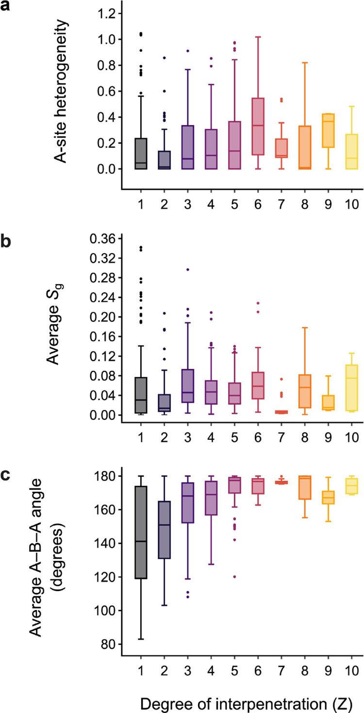
Distributions of geometric property indicators for increasing degrees of interpenetration, Z, of the dia-based MOFs in the data set. The figure shows (a) A-site heterogeneity (eq 5), (b) average angular component, S_g, of the Chau–Hardwick order parameter, and (c) average A−B−A angle.

We note that the majority of dia MOFs have locally homogeneous A sites, and this homogeneity does not appear to substantially depend on the degree of interpenetration (Figure 6a). Similarly, the distribution of the average S_g does not show a clear correlation with the degree of interpenetration (Figure 6b). There is, in contrast, a much stronger correlation with the A−B−A angle: as the degree of interpenetration increases, the average A−B−A angle tends toward 180° (Figure 6c). This makes intuitive sense when one considers that longer, “rod-like” ligands gives rise to greater void space and therefore enable a greater degree of interpenetration, which is consistent with the synthetic approach of employing longer spacer ligands to target higher degrees of interpenetration.⁶⁸⁻⁷⁰ It may be inferred from these distributions that the A sites maintain a similar environment, irrespective of the degree of interpenetration, whereas the linker geometry plays a crucial role in determining this property.

Finally, we extend this quantitative analysis to all topologies that occur at least five times in the data set, plotting the distribution of A-site heterogeneity values in the respective structures in Figure 7.

Figure 7.

Distributions of A-site heterogeneity (eq 5) for all structures in the data set for which the topology occurs ≥5 times. Three example MOFs are highlighted with coarse-grained structural representations, CSD refcodes, and the corresponding topology symbol and are discussed in the text.

The qzd structures have a distinctly narrow distribution of A-site heterogeneity values, which reinforces the hypothesis that the separation from the main body of structures in the t-SNE and UMAP embeddings (Figure 4) is a skewing of the visualization as a result of duplicate structures. It is also interesting to note that the zni topology has a narrow A-site heterogeneity distribution at a relatively high average value, which likely contributes to the separation of the zni structures.

Figure 7 highlights examples of topologies with particularly low (qzd) and particularly high (4T13, pts, and 2#pts) A-site heterogeneity, for which illustrative coarse-grained and scaled crystal structures are visualized. The structures with pts and 2#pts topology (which are related by increasing from a single to twofold interpenetrated net) all contain both tetrahedral and square planar geometries about different A sites, typically by combining Zn (tetrahedral geometric preference) with any of Ni, Cu, Pt, or Pd (square-planar geometric preference). Some frameworks have Cu in both the tetrahedral and square-planar sites of the pts framework. When combined with Au, Cu/Ag occupy the tetrahedral sites in the 2#pts framework. One might consider attempting to target these pts topologies, therefore, by selecting metals with the appropriate geometric preferences demanded by the framework.

The high degree of heterogeneity in the 4T13 frameworks can be ascribed to a tension between the differing lengths of two organic linkers, on the one hand, and the additional flexibility afforded using two linkers, on the other hand (cf. DEBWAK in Figure 7). The 4T13 frameworks have a short linker (e.g., isophthalate in DEBWAK) and a long-chain, flexible organic linker (e.g., N,N′-bis(pyridin-4-yl)-2,2′-bipyridine-5,5′-dicarboxamide in DEBWAK).^71,72 The resultant framework has 1-D helical chains that cross each other to create a 2-D molecular braid with geometrically distinct Zn sites. Automated, quantitative analyses such as those exemplified in Figures 6 and 7 should be a helpful part of the methodology used in future work for understanding the geometric and structural diversity in databases of materials.

Conclusions

We have studied the structures of AB₂ MOFs containing a diverse set of two-connected organic linkers. By coupling a cg-SOAP approach to different embedding schemes, we have visualized and analyzed the geometric diversity in a database of MOF structures. With the aid of cluster analysis, the structure maps of the AB₂ MOF configuration space can be better understood. Here, we have focused on clustering within the low-dimensional embedding and demonstrated how the location of structures in the map was consistent with the grouping of structures with similar structural properties. We described the cg-SOAP and visualization methodology implemented in a Python package and validated the routines by confirming that the underlying net was correct, using ToposPro software. We anticipate that the methodology described in this work will be useful in visualizing, analyzing, and understanding the geometric diversity in larger MOF data sets, to which we will dedicate future work.

Computational Details

Our code imports functionality from Pymatgen (the version used for the present work was 2020.12.31),⁴¹ the atomic simulation environment (ASE) (version 3.19.0),⁷³ and NetworkX (version 2.3)⁴⁷ for structure processing tasks. The SOAP implementation is imported from DScribe (version 0.4.0).⁷⁴ The Scikit-learn (version 0.21.3)⁷⁵ implementation of MDS and t-SNE and the stand-alone UMAP implementation (version 0.4.2) are used for dimensionality reduction. The Scikit-learn implementation of affinity propagation was used for cluster analysis. References for the algorithms themselves are given in the main text.

All structures were uniformly scaled to a minimum r(A−B) bond distance of unity. We computed SOAP vectors using the polynomial basis functions implemented in DScribe, with a radial cutoff of r_cut = 2.5, smoothness of σ = 0.2, and atomic neighbor density expansion of up to n_max = 10, l_max = 9 (as in ref (39)). (Note that here we do not include units for r_cut and σ because we have rescaled all structures.)

In order to assist the comparison of embedding schemes in Figure 4, the MDS coordinates were reflected in the x-axis and the UMAP coordinates were rotated 90° clockwise.

In terms of technical comparisons of the different algorithms, it is worth mentioning the relative times taken for the code to execute. All three algorithms could be performed on a standard MacBook Pro (1.4 GHz Quad-Core Intel Core i5 processor; 8 GB memory). The absolute times for MDS, t-SNE, and UMAP calculations were 98, 348, and 22 s, respectively. Hence, UMAP outperforms the other two embedding schemes for this particular purpose. It should be noted that a particularly low learning rate (5) was chosen for t-SNE because this was found to better capture the structure of the data (based on visual inspection of the relative “tightness” of clustering: smeared-out clusters can often be a sign that the algorithm has ended before reaching convergence). For future work on larger data sets, UMAP might therefore be preferred over t-SNE for its faster execution time.

The absolute positions of data points in the structure maps will depend slightly on the specific parameters chosen (and on numerical issues), particularly for t-SNE and UMAP; however, the global trends and interpretation of the visualizations were found to remain consistent for different choices of embedding parameters.

Data and Code Availability

The CHIC Python package described in this work is openly available online at https://github.com/tcnicholas/chic; the repository includes a tutorial (in the Jupyter notebook format) for the processing and coarse-graining of an example structure. The code is under ongoing development, and therefore, we have also deposited a copy of the specific version used to generate the figures in the present work at https://doi.org/10.5281/zenodo.5271082. The full data set of coarse-grained structures is available from the same Zenodo link.

Supporting Information Available

The Supporting Information is available free of charge at https://pubs.acs.org/doi/10.1021/acs.chemmater.1c02439.

• CSD reference codes; journal references; chemical formulae; chemical names; underlying net topology names; degrees of interpenetration; space groups; geometric densities; average angular components of the Chau-Hardwick order parameter; average A−B−A angles; and label of the cluster to which each structure in Figures 3 and 5 belongs (XLSX)

The authors declare no competing financial interest.

References

- Groom C. R.; Bruno I. J.; Lightfoot M. P.; Ward S. C. The Cambridge Structural Database. Acta Crystallogr., Sect. B: Struct. Sci., Cryst. Eng. Mater. 2016, 72, 171–179. 10.1107/s2052520616003954. [DOI] [PMC free article] [PubMed] [Google Scholar]
- Zagorac D.; Müller H.; Ruehl S.; Zagorac J.; Rehme S. Recent developments in the Inorganic Crystal Structure Database: theoretical crystal structure data and related features. J. Appl. Cryst. 2019, 52, 918–925. 10.1107/s160057671900997x. [DOI] [PMC free article] [PubMed] [Google Scholar]
- Butler K. T.; Davies D. W.; Cartwright H.; Isayev O.; Walsh A. Machine learning for molecular and materials science. Nature 2018, 559, 547–555. 10.1038/s41586-018-0337-2. [DOI] [PubMed] [Google Scholar]
- Jablonka K. M.; Ongari D.; Moosavi S. M.; Smit B. Big-Data Science in Porous Materials: Materials Genomics and Machine Learning. Chem. Rev. 2020, 120, 8066–8129. 10.1021/acs.chemrev.0c00004. [DOI] [PMC free article] [PubMed] [Google Scholar]
- Rosen A. S.; Iyer S. M.; Ray D.; Yao Z.; Aspuru-Guzik A.; Gagliardi L.; Notestein J. M.; Snurr R. Q. Machine learning the quantum-chemical properties of metal-organic frameworks for accelerated materials discovery. Matter 2021, 4, 1578–1597. 10.1016/j.matt.2021.02.015. [DOI] [PMC free article] [PubMed] [Google Scholar]
- Eddaoudi M.; Moler D. B.; Li H.; Chen B.; Reineke T. M.; O’Keeffe M.; Yaghi O. M. Modular Chemistry: Secondary Building Units as a Basis for the Design of Highly Porous and Robust Metal–Organic Carboxylate Frameworks. Acc. Chem. Res. 2001, 34, 319–330. 10.1021/ar000034b. [DOI] [PubMed] [Google Scholar]
- Yaghi O. M.; O’Keeffe M.; Ockwig N. W.; Chae H. K.; Eddaoudi M.; Kim J. Reticular synthesis and the design of new materials. Nature 2003, 423, 705–714. 10.1038/nature01650. [DOI] [PubMed] [Google Scholar]
- Long J. R.; Yaghi O. M. The pervasive chemistry of metal-organic frameworks. Chem. Soc. Rev. 2009, 38, 1213–1214. 10.1039/b903811f. [DOI] [PubMed] [Google Scholar]
- Tranchemontagne D. J.; Mendoza-Cortés J. L.; O’Keeffe M.; Yaghi O. M. Secondary building units, nets and bonding in the chemistry of metal-organic frameworks. Chem. Soc. Rev. 2009, 38, 1257–1283. 10.1039/b817735j. [DOI] [PubMed] [Google Scholar]
- Blatov V. A.; Shevchenko A. P.; Proserpio D. M. Applied Topological Analysis of Crystal Structures with the Program Package ToposPro. Cryst. Growth Des. 2014, 14, 3576–3586. 10.1021/cg500498k. [DOI] [Google Scholar]
- Delgado-Friedrichs O.; O’Keeffe M. Identification of and symmetry computation for crystal nets. Acta Crystallogr., Sect. A: Found. Crystallogr. 2003, 59, 351–360. 10.1107/s0108767303012017. [DOI] [PubMed] [Google Scholar]
- Amombo Noa F. M.; Svensson Grape E.; Brülls S. M.; Cheung O.; Malmberg P.; Inge A. K.; McKenzie C. J.; Mårtensson J.; Öhrström L. Metal-Organic Frameworks with Hexakis(4-carboxyphenyl)benzene: Extensions to Reticular Chemistry and Introducing Foldable Nets. J. Am. Chem. Soc. 2020, 142, 9471–9481. 10.1021/jacs.0c02984. [DOI] [PMC free article] [PubMed] [Google Scholar]
- Shevchenko A. P.; Alexandrov E. V.; Golov A. A.; Blatova O. A.; Duyunova A. S.; Blatov V. A. Topology versus porosity: what can reticular chemistry tell us about free space in metal-organic frameworks?. Chem. Commun. 2020, 56, 9616–9619. 10.1039/d0cc04004e. [DOI] [PubMed] [Google Scholar]
- Ortiz A. U.; Boutin A.; Fuchs A. H.; Coudert F.-X. Anisotropic Elastic Properties of Flexible Metal-Organic Frameworks: How Soft are Soft Porous Crystals?. Phys. Rev. Lett. 2012, 109, 195502. 10.1103/physrevlett.109.195502. [DOI] [PubMed] [Google Scholar]
- Ortiz A. U.; Boutin A.; Fuchs A. H.; Coudert F.-X. Metal-organic frameworks with wine-rack motif: What determines their flexibility and elastic properties?. J. Chem. Phys. 2013, 138, 174703. 10.1063/1.4802770. [DOI] [PubMed] [Google Scholar]
- Eddaoudi M.; Kim J.; Rosi N.; Vodak D.; Wachter J.; O’Keeffe M.; Yaghi O. M. Systematic Design of Pore Size and Functionality in Isoreticular MOFs and Their Application in Methane Storage. Science 2002, 295, 469–472. 10.1126/science.1067208. [DOI] [PubMed] [Google Scholar]
- Alezi D.; Belmabkhout Y.; Suyetin M.; Bhatt P. M.; Weseliński Ł. J.; Solovyeva V.; Adil K.; Spanopoulos I.; Trikalitis P. N.; Emwas A.-H.; Eddaoudi M. MOF Crystal Chemistry Paving the Way to Gas Storage Needs: Aluminum-Based soc-MOF for CH4, O2, and CO2 Storage. J. Am. Chem. Soc. 2015, 137, 13308–13318. 10.1021/jacs.5b07053. [DOI] [PMC free article] [PubMed] [Google Scholar]
- Chen Z.; Weseliński Ł. J.; Adil K.; Belmabkhout Y.; Shkurenko A.; Jiang H.; Bhatt P. M.; Guillerm V.; Dauzon E.; Xue D.-X.; O’Keeffe M.; Eddaoudi M. Applying the Power of Reticular Chemistry to Finding the Missing alb-MOF Platform Based on the (6,12)-Coordinated Edge-Transitive Net. J. Am. Chem. Soc. 2017, 139, 3265–3274. 10.1021/jacs.7b00219. [DOI] [PubMed] [Google Scholar]
- Collings I. E.; Tucker M. G.; Keen D. A.; Goodwin A. L. Geometric switching of linear to area negative thermal expansion in uniaxial metal-organic frameworks. CrystEngComm 2014, 16, 3498–3506. 10.1039/c3ce42165a. [DOI] [Google Scholar]
- Sadeghi A.; Ghasemi S. A.; Schaefer B.; Mohr S.; Lill M. A.; Goedecker S. Metrics for measuring distances in configuration spaces. J. Chem. Phys. 2013, 139, 184118. 10.1063/1.4828704. [DOI] [PubMed] [Google Scholar]
- Zhu L.; Amsler M.; Fuhrer T.; Schaefer B.; Faraji S.; Rostami S.; Ghasemi S. A.; Sadeghi A.; Grauzinyte M.; Wolverton C.; Goedecker S. A fingerprint based metric for measuring similarities of crystalline structures. J. Chem. Phys. 2016, 144, 034203. 10.1063/1.4940026. [DOI] [PubMed] [Google Scholar]
- Musil F.; Grisafi A.; Bartók A. P.; Ortner C.; Csányi G.; Ceriotti M. Physics-Inspired Structural Representations for Molecules and Materials. Chem. Rev. 2021, 121, 9759–9815. 10.1021/acs.chemrev.1c00021. [DOI] [PubMed] [Google Scholar]
- Behler J. Atom-centered symmetry functions for constructing high-dimensional neural network potentials. J. Chem. Phys. 2011, 134, 074106. 10.1063/1.3553717. [DOI] [PubMed] [Google Scholar]
- Rupp M.; Tkatchenko A.; Müller K.-R.; von Lilienfeld O. A. Fast and Accurate Modeling of Molecular Atomization Energies with Machine Learning. Phys. Rev. Lett. 2012, 108, 058301. 10.1103/PhysRevLett.108.058301. [DOI] [PubMed] [Google Scholar]
- Isayev O.; Oses C.; Toher C.; Gossett E.; Curtarolo S.; Tropsha A. Universal fragment descriptors for predicting properties of inorganic crystals. Nat. Commun. 2017, 8, 15679. 10.1038/ncomms15679. [DOI] [PMC free article] [PubMed] [Google Scholar]
- Willatt M. J.; Musil F.; Ceriotti M. Feature optimization for atomistic machine learning yields a data-driven construction of the periodic table of the elements. Phys. Chem. Chem. Phys. 2018, 20, 29661–29668. 10.1039/c8cp05921g. [DOI] [PubMed] [Google Scholar]
- Willatt M. J.; Musil F.; Ceriotti M. Atom-density representations for machine learning. J. Chem. Phys. 2019, 150, 154110. 10.1063/1.5090481. [DOI] [PubMed] [Google Scholar]
- Bartók A. P.; Kondor R.; Csányi G. On representing chemical environments. Phys. Rev. B 2013, 87, 184115. 10.1103/physrevb.87.184115. [DOI] [Google Scholar]
- De S.; Bartók A. P.; Csányi G.; Ceriotti M. Comparing molecules and solids across structural and alchemical space. Phys. Chem. Chem. Phys. 2016, 18, 13754–13769. 10.1039/c6cp00415f. [DOI] [PubMed] [Google Scholar]
- Moosavi S. M.; Jablonka K. M.; Smit B. The Role of Machine Learning in the Understanding and Design of Materials. J. Am. Chem. Soc. 2020, 142, 20273–20287. 10.1021/jacs.0c09105. [DOI] [PMC free article] [PubMed] [Google Scholar]
- Moosavi S. M.; Nandy A.; Jablonka K. M.; Ongari D.; Janet J. P.; Boyd P. G.; Lee Y.; Smit B.; Kulik H. J. Understanding the diversity of the metal-organic framework ecosystem. Nat. Commun. 2020, 11, 4068. 10.1038/s41467-020-17755-8. [DOI] [PMC free article] [PubMed] [Google Scholar]
- Cheng B.; Griffiths R.-R.; Wengert S.; Kunkel C.; Stenczel T.; Zhu B.; Deringer V. L.; Bernstein N.; Margraf J. T.; Reuter K.; Csanyi G. Mapping Materials and Molecules. Acc. Chem. Res. 2020, 53, 1981–1991. 10.1021/acs.accounts.0c00403. [DOI] [PubMed] [Google Scholar]
- Pulido A.; et al. Functional materials discovery using energy-structure-function maps. Nature 2017, 543, 657–664. 10.1038/nature21419. [DOI] [PMC free article] [PubMed] [Google Scholar]
- Engel E. A.; Anelli A.; Ceriotti M.; Pickard C. J.; Needs R. J. Mapping uncharted territory in ice from zeolite networks to ice structures. Nat. Commun. 2018, 9, 2173. 10.1038/s41467-018-04618-6. [DOI] [PMC free article] [PubMed] [Google Scholar]
- Yang J.; De S.; Campbell J. E.; Li S.; Ceriotti M.; Day G. M. Large-Scale Computational Screening of Molecular Organic Semiconductors Using Crystal Structure Prediction. Chem. Mater. 2018, 30, 4361–4371. 10.1021/acs.chemmater.8b01621. [DOI] [Google Scholar]
- Musil F.; De S.; Yang J.; Campbell J. E.; Day G. M.; Ceriotti M. Machine learning for the structure-energy-property landscapes of molecular crystals. Chem. Sci. 2018, 9, 1289–1300. 10.1039/c7sc04665k. [DOI] [PMC free article] [PubMed] [Google Scholar]
- Helfrecht B. A.; Semino R.; Pireddu G.; Auerbach S. M.; Ceriotti M. A new kind of atlas of zeolite building blocks. J. Chem. Phys. 2019, 151, 154112. 10.1063/1.5119751. [DOI] [PubMed] [Google Scholar]
- Zhao C.; Chen L.; Che Y.; Pang Z.; Wu X.; Lu Y.; Liu H.; Day G. M.; Cooper A. I. Digital navigation of energy-structure-function maps for hydrogen-bonded porous molecular crystals. Nat. Commun. 2021, 12, 817. 10.1038/s41467-021-21091-w. [DOI] [PMC free article] [PubMed] [Google Scholar]
- Nicholas T. C.; Goodwin A. L.; Deringer V. L. Understanding the geometric diversity of inorganic and hybrid frameworks through structural coarse-graining. Chem. Sci. 2020, 11, 12580–12587. 10.1039/d0sc03287e. [DOI] [PMC free article] [PubMed] [Google Scholar]
- Jablonka K. M.; Ongari D.; Moosavi S. M.; Smit B. Using collective knowledge to assign oxidation states of metal cations in metal-organic frameworks. Nat. Chem. 2021, 13, 771–777. 10.1038/s41557-021-00717-y. [DOI] [PubMed] [Google Scholar]
- Ong S. P.; Richards W. D.; Jain A.; Hautier G.; Kocher M.; Cholia S.; Gunter D.; Chevrier V. L.; Persson K. A.; Ceder G. Python Materials Genomics (pymatgen): A robust, open-source python library for materials analysis. Comput. Mater. Sci. 2013, 68, 314–319. 10.1016/j.commatsci.2012.10.028. [DOI] [Google Scholar]
- Heller S. R.; McNaught A.; Pletnev I.; Stein S.; Tchekhovskoi D. InChI, the IUPAC International Chemical Identifier. J. Cheminf. 2015, 7, 23. 10.1186/s13321-015-0068-4. [DOI] [PMC free article] [PubMed] [Google Scholar]
- Zhang J.; Wu T.; Zhou C.; Chen S.; Feng P.; Bu X. Zeolitic Boron Imidazolate Frameworks. Angew. Chem., Int. Ed. 2009, 48, 2542–2545. 10.1002/anie.200804169. [DOI] [PMC free article] [PubMed] [Google Scholar]
- Yaghi O. M.; Li G.; Li H. Selective binding and removal of guests in a microporous metal-organic framework. Nature 1995, 378, 703–706. 10.1038/378703a0. [DOI] [Google Scholar]
- Zimmermann N. E. R.; Jain A. Local structure order parameters and site fingerprints for quantification of coordination environment and crystal structure similarity. RSC Adv. 2020, 10, 6063–6081. 10.1039/c9ra07755c. [DOI] [PMC free article] [PubMed] [Google Scholar]
- Joshi S. Y.; Deshmukh S. A. A review of advancements in coarse-grained molecular dynamics simulations. Mol. Simul. 2021, 47, 786. 10.1080/08927022.2020.1828583. [DOI] [Google Scholar]
- Hagberg A. A.; Schult D. A.; Swart P. J.. Exploring Network Structure, Dynamics, and Function using NetworkX. Proceedings of the 7th Python in Science Conference; Los Alamos National Lab.: Pasadena, CA USA, 2008; pp 11–15.
- Bernstein N.; Csányi G.; Deringer V. L. De novo exploration and self-guided learning of potential-energy surfaces. npj Comput. Mater. 2019, 5, 99. 10.1038/s41524-019-0236-6. [DOI] [Google Scholar]
- Torgerson W. S. Multidimensional scaling: I. Theory and method. Psychometrika 1952, 17, 401–419. 10.1007/bf02288916. [DOI] [Google Scholar]
- Van der Maaten L.; Hinton G. Visualizing Data using t-SNE. J. Mach. Learn. Res. 2008, 9, 2579–2605. [Google Scholar]
- McInnes L.; Healy J.; Saul N.; Großberger L. UMAP: Uniform Manifold Approximation and Projection. J. Open Source Software 2018, 3, 861. 10.21105/joss.00861. [DOI] [Google Scholar]
- Alexandrov E. V.; Blatov V. A.; Kochetkov A. V.; Proserpio D. M. Underlying nets in three-periodic coordination polymers: topology, taxonomy and prediction from a computer-aided analysis of the Cambridge Structural Database. CrystEngComm 2011, 13, 3947–3958. 10.1039/c0ce00636j. [DOI] [Google Scholar]
- Alexandrov E. V.; Shevchenko A. P.; Blatov V. A. Topological Databases: Why Do We Need Them for Design of Coordination Polymers?. Cryst. Growth Des. 2019, 19, 2604–2614. 10.1021/acs.cgd.8b01721. [DOI] [Google Scholar]
- Chau P.-L.; Hardwick A. J. A new order parameter for tetrahedral configurations. Mol. Phys. 1998, 93, 511–518. 10.1080/002689798169195. [DOI] [Google Scholar]
- Steinhardt P. J.; Nelson D. R.; Ronchetti M. Bond-orientational order in liquids and glasses. Phys. Rev. B 1983, 28, 784–805. 10.1103/physrevb.28.784. [DOI] [Google Scholar]
- Lechner W.; Dellago C. Accurate determination of crystal structures based on averaged local bond order parameters. J. Chem. Phys. 2008, 129, 114707. 10.1063/1.2977970. [DOI] [PubMed] [Google Scholar]
- Frey B. J.; Dueck D. Clustering by Passing Messages Between Data Points. Science 2007, 315, 972–976. 10.1126/science.1136800. [DOI] [PubMed] [Google Scholar]
- Schölkopf B.; Smola A.; Müller K.-R. Nonlinear Component Analysis as a Kernel Eigenvalue Problem. Neural Comput. 1998, 10, 1299–1319. 10.1162/089976698300017467. [DOI] [Google Scholar]
- Helfrecht B. A.; Cersonsky R. K.; Fraux G.; Ceriotti M. Structure-property maps with Kernel principal covariates regression. Mach. Learn.: Sci. Technol. 2020, 1, 045021. 10.1088/2632-2153/aba9ef. [DOI] [Google Scholar]
- Ying S.-M.; Mao J.-G.; Sun Y.-Q.; Zeng H.-Y.; Dong Z.-C. Syntheses and crystal structures of three open-frameworks of metal succinates containing a 4,4′-bipyridine ligand. Polyhedron 2003, 22, 3097–3103. 10.1016/s0277-5387(03)00467-4. [DOI] [Google Scholar]
- Wu S.-T.; Wu Y.-R.; Kang Q.-Q.; Zhang H.; Long L.-S.; Zheng Z.; Huang R.-B.; Zheng L.-S. Chiral Symmetry Breaking by Chemically Manipulating Statistical Fluctuation in Crystallization. Angew. Chem., Int. Ed. 2007, 46, 8475–8479. 10.1002/anie.200703443. [DOI] [PubMed] [Google Scholar]
- Wharmby M. T.; Henke S.; Bennett T. D.; Bajpe S. R.; Schwedler I.; Thompson S. P.; Gozzo F.; Simoncic P.; Mellot-Draznieks C.; Tao H.; Yue Y.; Cheetham A. K. Extreme Flexibility in a Zeolitic Imidazolate Framework: Porous to Dense Phase Transition in Desolvated ZIF-4. Angew. Chem., Int. Ed. 2015, 54, 6447–6451. 10.1002/anie.201410167. [DOI] [PubMed] [Google Scholar]
- Widmer R. N.; Lampronti G. I.; Chibani S.; Wilson C. W.; Anzellini S.; Farsang S.; Kleppe A. K.; Casati N. P. M.; MacLeod S. G.; Redfern S. A. T.; Coudert F.-X.; Bennett T. D. Rich Polymorphism of a Metal-Organic Framework in Pressure-Temperature Space. J. Am. Chem. Soc. 2019, 141, 9330–9337. 10.1021/jacs.9b03234. [DOI] [PMC free article] [PubMed] [Google Scholar]
- Barthel S.; Alexandrov E. V.; Proserpio D. M.; Smit B. Distinguishing Metal-Organic Frameworks. Cryst. Growth Des. 2018, 18, 1738–1747. 10.1021/acs.cgd.7b01663. [DOI] [PMC free article] [PubMed] [Google Scholar]
- Jiang H.-L.; Makal T. A.; Zhou H.-C. Interpenetration control in metal-organic frameworks for functional applications. Coord. Chem. Rev. 2013, 257, 2232–2249. 10.1016/j.ccr.2013.03.017. [DOI] [Google Scholar]
- Verma G.; Butikofer S.; Kumar S.; Ma S. Regulation of the Degree of Interpenetration in Metal-Organic Frameworks. Top. Curr. Chem. 2019, 378, 4. 10.1007/s41061-019-0268-x. [DOI] [PubMed] [Google Scholar]
- Gupta M.; Vittal J. J. Control of interpenetration and structural transformations in the interpenetrated MOFs. Coord. Chem. Rev. 2021, 435, 213789. 10.1016/j.ccr.2021.213789. [DOI] [Google Scholar]
- Carlucci L.; Ciani G.; Proserpio D. M.; Rizzato S. Three Novel Interpenetrating Diamondoid Networks from Self-Assembly of 1,12-Dodecanedinitrile with Silver(I) Salts. Chem.—Eur. J. 2002, 8, 1519–1526. 10.1002/1521-3765(20020402)8:7<1519::aid-chem1519>3.0.co;2-5. [DOI] [PubMed] [Google Scholar]
- Tian A.-X.; Ying J.; Peng J.; Sha J.-Q.; Pang H.-J.; Zhang P.-P.; Chen Y.; Zhu M.; Su Z.-M. Tuning the Dimensionality of the Coordination Polymer Based on Polyoxometalate by Changing the Spacer Length of Ligands. Cryst. Growth Des. 2008, 8, 3717–3724. 10.1021/cg800353y. [DOI] [Google Scholar]
- He Y.-P.; Tan Y.-X.; Zhang J. Deliberate design of a neutral heterometallic organic framework containing a record 25-fold interpenetrating diamondoid network. CrystEngComm 2012, 14, 6359–6361. 10.1039/c2ce25605c. [DOI] [Google Scholar]
- Jacobs T.; Clowes R.; Cooper A. I.; Hardie M. J. A Chiral, Self-Catenating and Porous Metal-Organic Framework and its Post-Synthetic Metal Uptake. Angew. Chem., Int. Ed. 2012, 51, 5192–5195. 10.1002/anie.201200758. [DOI] [PubMed] [Google Scholar]
- Luo F.; Wang M.-S.; Luo M.-B.; Sun G.-M.; Song Y.-M.; Li P.-X.; Guo G.-C. Functionalizing the pore wall of chiral porous metal-organic frameworks by distinct -H, -OH, -NH2, -NO2, -COOH shutters showing selective adsorption of CO2, tunable photoluminescence, and direct white-light emission. Chem. Commun. 2012, 48, 5989–5991. 10.1039/c2cc32103c. [DOI] [PubMed] [Google Scholar]
- Hjorth Larsen A.; et al. The atomic simulation environment-a Python library for working with atoms. J. Phys.: Condens. Matter 2017, 29, 273002. 10.1088/1361-648x/aa680e. [DOI] [PubMed] [Google Scholar]
- Himanen L.; Jäger M. O. J.; Morooka E. V.; Federici Canova F.; Ranawat Y. S.; Gao D. Z.; Rinke P.; Foster A. S. DScribe: Library of descriptors for machine learning in materials science. Comput. Phys. Commun. 2020, 247, 106949. 10.1016/j.cpc.2019.106949. [DOI] [Google Scholar]
- Pedregosa F.; et al. Scikit-learn: Machine Learning in Python. J. Mach. Learn. Res. 2011, 12, 2825–2830. [Google Scholar]
Associated Data
This section collects any data citations, data availability statements, or supplementary materials included in this article.
Supplementary Materials
Data Availability Statement