A reinforcement learning application of a guided Monte Carlo Tree Search algorithm for beam orientation selection in radiation therapy

Abstract

Current beam orientation optimization algorithms for radiotherapy, such as column generation (CG), are typically heuristic or greedy in nature because of the size of the combinatorial problem, which leads to suboptimal solutions. We propose a reinforcement learning strategy using Monte Carlo Tree Search that can find a better beam orientation set in less time than CG. We utilize a reinforcement learning structure involving a supervised learning network to guide the Monte Carlo Tree Search and to explore the decision space of beam orientation selection problems. We previously trained a deep neural network (DNN) that takes in the patient anatomy, organ weights, and current beams, then approximates beam fitness values to indicate the next best beam to add. Here, we use this DNN to probabilistically guide the traversal of the branches of the Monte Carlo decision tree to add a new beam to the plan. To assess the feasibility of the algorithm, we used a test set of 13 prostate cancer patients, distinct from the 57 patients originally used to train and validate the DNN, to solve for 5-beam plans. To show the strength of the guided Monte Carlo tree search (GTS) compared to other search methods, we also provided the performances of guided search, uniform tree search and random search algorithms. On average, GTS outperformed all other methods. It found a better solution than CG in 237 seconds on average, compared to 360 seconds for CG, and outperformed all other methods in finding a solution with a lower objective function value in less than 1000 seconds. Using our guided tree search (GTS) method, we could maintain planning target volume (PTV) coverage within 1% error similar to CG, while reducing the organ-at-risk (OAR) mean dose for body, rectum, left and right femoral heads; mean dose to bladder was 1% higher with GTS than with CG.

I. Introduction

Radiation therapy is one of the main modalities to cure cancer and is used in over half of cancer treatments, either as a standalone therapy or in conjunction with another modality, such as surgery or chemotherapy.[1] For intensity-modulated radiation therapy (IMRT), the patient’s body is irradiated from fixed beam locations around the body, and the radiation field is modulated at each beam position by multileaf collimators (MLC).[2] In IMRT, the optimal choice of beam orientations has a direct impact on the treatment plan quality, which influences the final treatment outcome [3] and, ultimately, patients’ quality of life. Current clinical practice is to select the beam orientations either by protocol or manually by the treatment planner.[3, 4] Beam orientation optimization (BOO) methods solve for a suitable set of beam angles by minimizing an objective function to a local minimum.[5, 6] BOO has been studied extensively in radiation therapy procedures, for both coplanar[3, 5–29] and noncoplanar [3, 5, 9, 10, 23, 26, 29–38] IMRT, as well as for intensity-modulated proton therapy (IMPT)[39–44] over the past three decades. However, BOO methods have not been widely adopted because of their high computational cost and complexity, as they involve a large-scale NP hard combinatorial problem.[34, 45] Despite extensive research, there are still no clinically practical beam orientation selection algorithms because the procedure is computationally expensive and time intensive, and the final solutions are usually sub-optimal, so BOO remains a challenge for treatment planning.

To measure the quality of a BOO solution, the dose influence array of each potential beam orientation must be calculated. The dose influence array for one beam associates all the individual beamlets in the fluence map with the voxels of the patient’s body. This calculation is time-consuming, and it requires a large amount of memory for optimization. To manage the limited capacity of computational resources, the treatment planning process, after defining the objective function, may be divided into two major steps: 1) finding a suitable set of beam orientations, and 2) solving the fluence map optimization (FMO)[6] problem for the selected beams. However, these two steps are not independent of each other: the quality of the BOO solution can be evaluated only after the FMO problem has been solved, and the FMO can be defined only after the BOO has been solved. Because of the non-convexity and large scale of the problem, researchers have considered dynamic programming methods that break the problem into a sequence of smaller problems. Column Generation (CG) is a successful algorithm specifically developed to solve complex problems such as BOO. Romeijn et al.[13] initially applied CG to radiotherapy to solve a direct aperture optimization (DAO) problem. Dong et al.[46] then proposed a greedy algorithm based on CG, which iteratively adds beam orientations until the desired number of beams has been reached. Rwigema et al.[47] used CG to find a set of 30 beam orientations for use in 4π treatment planning of stereotactic body radiation therapy (SBRT) for patients with recurrent, locally advanced, or metastatic head-and-neck cancers, to show the superiority of the 4π treatment plans over those created by volumetric modulated arc therapy (VMAT). Nguyen et al[48] used CG to solve the triplet beam orientation selection problem specific to MRI-guided Co-60 radiotherapy. Yu et al.[32] used an in-house CG algorithm to solve an integrated problem of beam orientation and fluence map optimization.

However, CG is a greedy algorithm that cannot guarantee optimal results and typically yields a sub-optimal solution. In addition, CG still takes as much as 560 seconds to suggest a 5-beam plan for prostate IMRT.[49] The aim of this work is to find a method that can explore a larger area of the BOO decision space to find higher quality solutions than those achieved by CG in a shorter amount of time. The method we propose here starts with a deep neural network that has been trained using CG as a supervisor. This network can mimic the behavior of CG by directly learning CG’s fitness evaluations of beam orientations via supervised learning. Our previous work presents the efficiency of this supervised network, which can propose a set of beam angles that is better than that proposed by CG in less than two seconds[49]. Given a set of already selected beams, this network will predict the fitness value of each beam, which is how much the beam will improve the objective function when added in the next iteration.

In this study, we extend our previous work and combine this trained supervised learning (SL) network with a reinforcement learning method called Monte Carlo Tree Search. We use these fitness values from the SL network as a guide to efficiently navigate the action space of the reinforcement learning tree. Specifically, this method provides the probability of selecting a beam in the search space of the tree at each iteration, so that the beam with the better likelihood to improve the objective function has the higher chance of being selected at each step. To evaluate our proposed method, we compared its performance against the state-of-the-art CG. We developed three additional combinations of guided and random search tree approaches for comparison.

II. Theoretical and Experimental Methods

The proposed method has a reinforcement learning structure involving a supervised learning network that guides Monte Carlo Tree Search to explore the beam orientation selection decision space.

This method, which we named guided Monte Carlo Tree Search (GTS), consists of two main phases: 1) supervised training a deep neural network (DNN) to predict the probability distribution for adding the next beam, based on patient anatomy, and 2) using this network for a guided Monte Carlo Tree Search method to explore a larger decision space more efficiently to find better solutions than CG. For the first phase, we use the CG implementation for BOO problems, where CG iteratively solves a sequence of Fluence Map Optimization (FMO) problems[6] by using a GPU-based Chambolle-Pock algorithm[50]; the results of the CG method are used to train a supervised neural network. For the second phase, which is the main focus of this work, we present a Monte Carlo Tree Search algorithm that uses the trained DNN. Each of these phases is presented in the following sections.

II.A. Supervised Training the Deep Neural Network

We developed a deep neural network (DNN) model that learns from column generation how to find fitness values for each beam based on the anatomical features of a patient and a set of structure weights for the planning target volume (PTV) and organs-at-risk (OARs). The greedy CG algorithm starts with an empty set of selected beams, then calculates the fitness value of each beam based on the optimality condition of the objective function shown in Equation 1

$$\underset{x}{\min }\frac{1}{2}{\sum }_{\forall s\in S}{w}_s^2{‖D_{s}x-p‖}_2^{2}s.t. x\ge 0$$ (1)

where w_s is the weight for structure s, which are pseudo-randomly generated between zero and one during the training process to generate many different scenarios. The value p is the prescription dose for each structure, which is assigned 1 for the PTV and 0 for OARs. At each iteration of CG, fitness values are calculated based on Karush–Kuhn–Tucker (KKT) conditions[51, 52] of a master problem, and they represent how much each beam would improve the objective function value. The beam with the highest fitness value is added to the selected beam set S. Then, FMO is performed for the selected beams, which affects the fitness value calculations for the next iteration. The process is repeated until the desired number of beams has been selected. The supervised DNN learns to mimic this behavior through training, as shown in Figure 1. Once trained, this DNN can efficiently provide a suitable set of beam angles in less than 2 seconds, as opposed to the 560 seconds that CG needs to solve the same problem. The details of the DNN structure and its training process are described in our previous work.[49]

Figure 1:

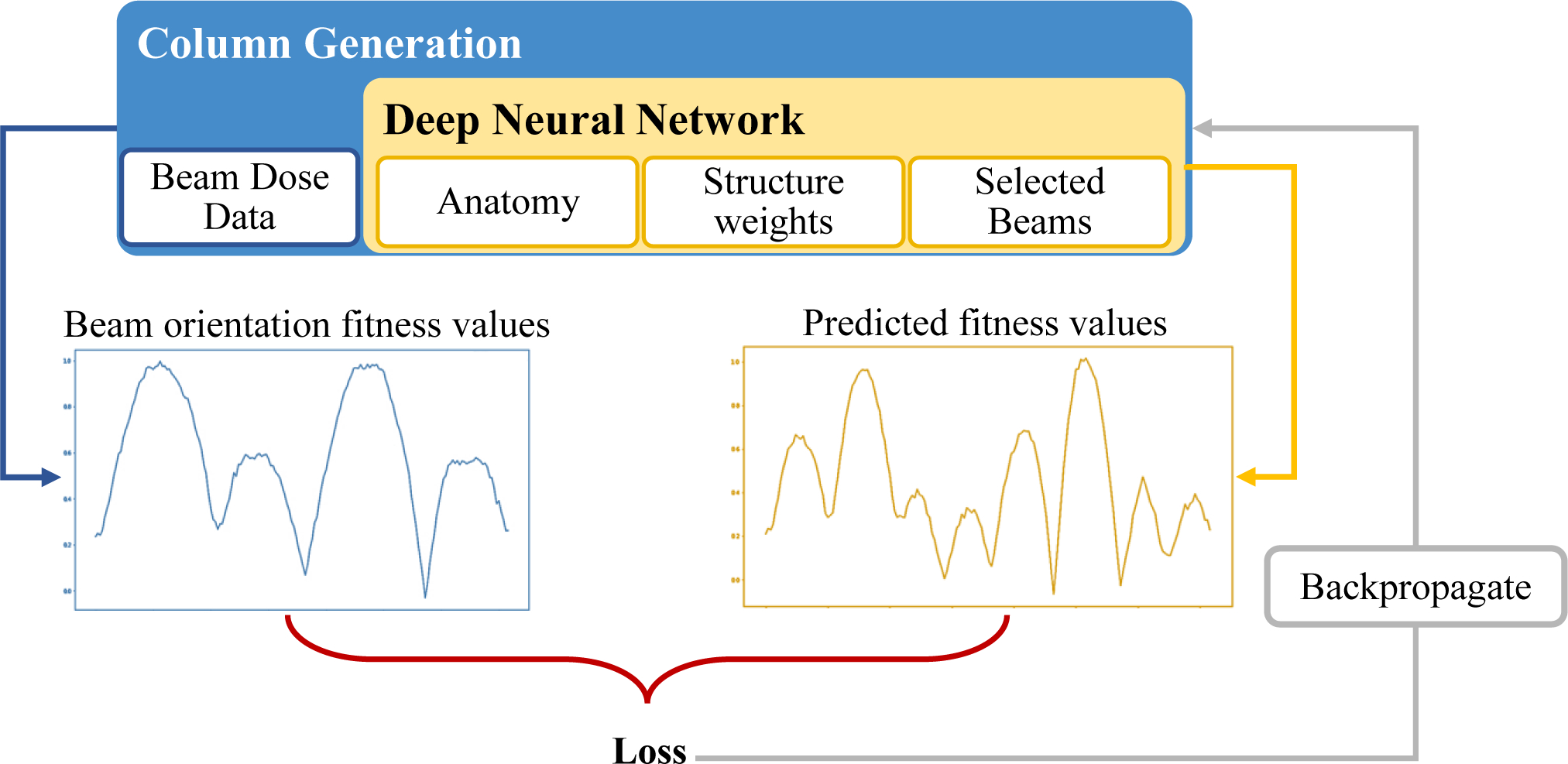
Schematic of the supervised training structure to predict beam orientation fitness values. Column Generation (“CG”) is the teacher, and deep neural network (“DNN”) is the trainee.

For this study, the patient anatomical features included the contoured structures (organs-at-risk) on images from patients with prostate cancer and the treatment planning weights assigned to each structure. We used the images of 70 prostate cancer patients for this research, each with 6 contours: planning target volume (PTV), body, bladder, rectum, and left and right femoral heads. We randomly selected 50 of these 70 patients to train the network and 7 patients to validate it. We used the images from the remaining 13 patients to test and apply the Monte Carlo Tree Search method.

II.B. Monte Carlo Tree Search

The pre-trained DNN probabilistically guides the traversal of the branches on the Monte Carlo decision tree to add a new beam to the plan. Each branch of the tree starts from the root as an empty set of beams and continues until it reaches the terminal state. After each complete plan (selection of 5 beams, in our case) has been explored, the FMO problem is solved; based on its solution, the probability distribution to select the next beam will be updated, using the reward function, in the backpropagation stage. Then, starting from the root, the exploration of the next plan will begin until the stopping criterion is met. Figure 2 shows an example of a tree search that has discovered seven plans so far.

Figure 2:

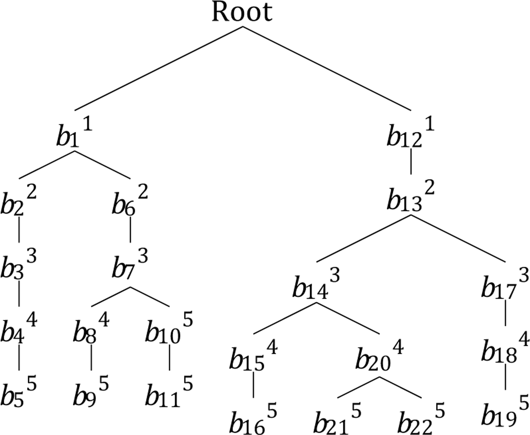
An example of guided tree search. Subscripts indicate the order in which a node is generated, and superscripts indicate the depth of the node in the tree.

II.B.1. Basics of Monte Carlo Tree Search

Monte Carlo Tree Search (MCTS) uses a decision tree to explore the decision space by randomly sampling from it.[53] The search process of MCTS consists of four steps: 1) node selection, 2) expansion, 3) simulation, and 4) backpropagation of the simulation result. To explain these processes in detail, we need to define some properties first:

State of the problem: includes patient’s anatomical features and a set of selected beam orientations (B). At the beginning of the planning, this set has no members, and it is updated throughout the solution procedure.

Actions: the selection of the next beam orientation to be added to set B, given the state of the problem.

Solution or terminal state: state of the problem in which the number of selected beam orientations (size of B) is the same as a predefined number of beams (N) chosen by the user. At this point, a feasible solution for the problem is generated.

Decision tree: The solution space of a set of discrete numbers—in this work, the beam orientations—especially with iterative structures, can be defined as a tree, where each node and branch represent the selection of one number and a subset of available numbers, respectively.

Node (Y): selection of one potential beam orientation.

Root (O): a node with an empty set of beam orientations. Every solution starts from the root.

Path: a unique connected sequence of nodes in a decision tree.

Branch (Q): a path originating from the root node. Each branch represents the iterative structure of the proposed method. The length of a branch is the number of nodes in that branch. In this work, a solution is a branch with size N + 1. There is only one branch from each root to any node in a tree.

Leaf: the last node of a branch. There is no exploration of the tree after a leaf is discovered.

Internal node: any node in a tree other than the root and the leaves.

The selection process in the proposed method is guided by a pre-trained DNN, as described in subsection II.A. This DNN is used to probabilistically guide the traversal of the branches on the Monte Carlo decision tree to add a new beam to the plan. At each node—starting from the root node—the DNN is called to predict an array of fitness values for each beam orientation (P). An element of this array P[i] represents the likelihood of selecting the i^th beam orientation. For example, if the number of potential beam orientations is 180, with 2° separation, Y would be an array of size 180, and P[2] is the likelihood of selecting the beam orientation in the 2^nd position of the potential beam orientations, P[2] = 4°. The expansion process happens after the selection process at internal nodes to further explore the tree and create child nodes. The traversal approach in the proposed method is depth first, which means that the branch of a node that is visited or created for the first time continues expanding until there are N +1 nodes in the branch. In this case, the selection and expansion processes overlap, because only one child node is created or visited at a time, though a node can be visited multiple times and several children can be generated from one node. The leaf node is the exception, as it does not have any children. Nodes in a branch must be unique, which means that a branch of each external node (Q) can be expanded only to nodes that are not already in the branch. In fact, the beam orientation optimization problem can be defined as a dynamic programming problem with the formula

$$G_k^S=S\cup \{k\}\cup G_{n^{\ast }}^{S\cup \left\{k\right\}}\mid n^{\ast }=\mathit{arg}\underset{n>k}{\max }{V}_{G_n^{S\cup \left\{k\right\}}}$$ (2)

where S is a set of indices for previously selected beams, k is the index of the currently selected beam, and $G_{n^{\ast }}^{S\cup \left\{k\right\}}$ is a subset of beams to be selected that has the highest reward value. Each simulation iteratively selects a predefined number of beams (N); in this work, N = 5. After each complete plan has been explored, the fluence map optimization problem is solved and used for the backpropagation step, which updates the probability distribution for beam selection.

II.B.2. Main Algorithm

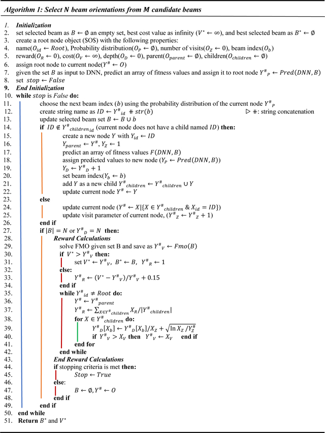
The details of the guided Monte Carlo Tree Search algorithm in the form of a pseudo-code are provided in Algorithm 1. Several properties of each node in the proposed tree are updated after the exploration of final states. To simplify the algorithm, these properties are addressed as variables, defined as follows:

Cost (Y_v): After a leaf is discovered, an FMO problem associated with the beams of that branch is solved, where the value of the FMO cost function is the value associated with its corresponding leaf. The cost value of all other nodes (other than leaves) in a tree is the average cost of its sub-branches. For example, in Figure 2, the cost value of node b₁¹ is the average cost of nodes b₂² and b₆².

Probability distribution (Y_P): an array of size 180 (the number of potential beam orientations), where the i^th element of this array represents the chance of improving the current cost value if the tree branches out by selecting the i^th beam. After a node is discovered in the tree, this distribution is populated by using DNN. After the first discovery of a node, Y_P is updated based on the reward values.

Reward (Y_R): a function of the node’s cost values and the best cost value ever discovered in the search process. The reward values are updated after each cost calculation and are calculated and updated by the reward calculation procedure defined in line 28 of Algorithm 1.

Depth (Y_D): the number of beam orientations selected after node Y is discovered.

Name (Y_id): a unique string value as id for each node. This value is the path from the root to node Y.

Beam Set (Y_B): the set of beams selected for a branch starting from the root and ending in node Y.

Parent (Y_parent): the node immediately preceding node Y in a branch from the root to Y. With the exception of the root node, all nodes in a tree have one parent.

Children (Y_children): the node(s) of the sub-branches that immediately proceed from node Y. With the exception of leaves, all nodes in a tree have at least one child.

II.C. Algorithms for performance comparison

We designed four frameworks to show the efficiency of the proposed GTS method by comparison:

Guided Tree Search (GTS): As presented in Algorithm 1. This framework used a pre-trained policy network to guide a Monte Carlo decision tree.

Guided Search (GuidS): This framework used the pre-trained network to search the decision space by iteratively choosing one beam based on the probabilities predicted by the policy network. Unlike GTS, the search policy is not updated as the search progresses. This process is detailed in Algorithm 2.

Random Sampling Tree Search (RTS): This algorithm is a simple Monte Carlo Tree Search method that starts with a uniform distribution to randomly select beam orientations, then updates the search policy as the tree search progresses. Note that all of the tree operations used in GTS are also used in this algorithm, but the tree search is not guided by a pre-trained policy network. This method is proposed to show the impact of using DNN to guide the decision tree.

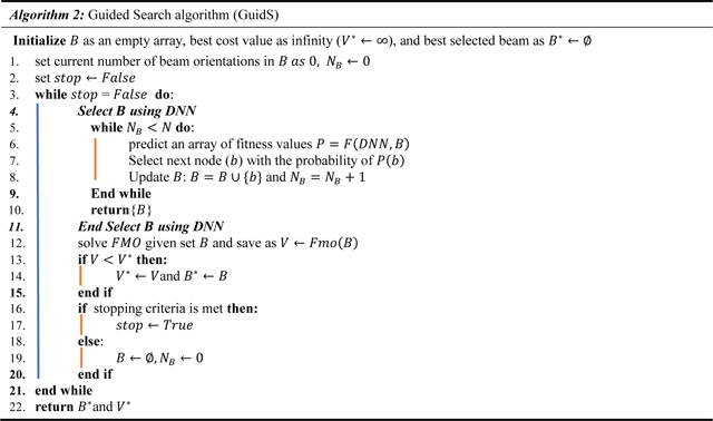
Random Search (RandS): This method searches the decision space with uniformly random probability until the stopping criterion is met. It randomly selects 5 beam orientations and solves the corresponding FMO problem. The search policy is not updated. Its procedure is close to Algorithm 2, but the “Select B using DNN” procedure is replaced by randomly selecting 5 unique beams.

II.D. Data

We used images from 70 patients with prostate cancer at 5 mm³ voxel size. The exact shape of each patient varied, but ranged from 80–168 rows, 124–261 columns, and 110–219 slices. Each image has 6 contours: PTV, body, bladder, rectum, left femoral head, and right femoral head. The segmentation masks for each structure were contoured by physicians and dosimetrists on the CT images during the clinical workflow. Additionally, the skin and shell¹ tuning structures were added during the fluence map optimization process to control high dose spillage and conformity in the body. The dose influence arrays were calculated for 70 patients, which included 180 candidate coplanar beams equidistantly spaced 2 degrees apart, and with a beamlet size of 2.5mm² at 100 cm isocenter. These dose influence data is then used to generate the various plans with varying beams through CG and FMO optimization. CG was implemented with a GPU-based Chambolle-Pock algorithm[50], a first-order primal-dual proximal-class algorithm, to create scenarios. The patients were divided randomly into two exclusive sets: 1) a model development set consisting of 57 patients, 50 for training and 7 for validation, and 2) a test data set consisting of 13 patients. The total number of scenarios created were, 6270 training and validation scenarios (10 five-beam plans for each of the 57 patients= 10 × 5 × 57, and then 12 randomly generated beam sets from zero input to 4 initial beam input scenarios = 12 × 5 × 57 . To generate multiple scenarios for each patients, other than randomly selecting the input beam set with sizes from zero to four, the weights of the structures are also generated pseudo randomly, as describes in the next paragraph) and 650 test scenarios (10 five-beam plans for each of the 13 test patients= 10 × 5 × 13). To feed into the model, the data is zero-padded and interpolated into a 64 × 64 × 64 shape, and the aspect ratio of original data is maintained by the zero padding. The DNN trained over 400 epochs, each with 2500 steps and a batch size of one.

We evaluated the performances of four methods: GTS, GuidS, RTS, and RandS, explained in subsection II.C. Two of these methods, GTS and GuidS, use the pre-trained DNN as a guidance network. We started with the images of 70 patients with prostate cancer, and we used the images of 57 of them to train and validate the DNN; therefore, we could not use them for testing in this project, to keep the proposed methods completely independent from the dataset used for training DNN. We used the images of the 13 patients that DNN had never seen before as the test set. Multiple scenarios can be generated for each patient, based on the weights assigned to patient’s structures for planning their treatments. We semi-randomly generated ten sets of weights for each patient. In total, we had 130 test plans across 13 test patients for comparison. All tests in this paper were performed on a computer with an Intel Core I7 processor at 3.6 GHz, 64 GB memory, and an NVIDIA GeForce GTX 1080 Ti GPU with 11 GB video memory.

The structure weight selection scheme is outlined as follows:

1. In 50% of the cases, we used a uniform distribution in the range of 0 to 0.1 to generate a weight for each OAR separately.

2. In 10% of the cases, we used a uniform distribution in the smaller range of 0 to 0.05 to select weights for OARs separately.

3. Finally, in 40% of the cases, we used specific ranges for each OAR. Bladder: [0,0.2], Rectum: [0,0.2], Right Femoral Head: [0,0.1], Left Femoral Head: [0,0.1], Shell: [0,0.1] and Skin: [0,0.3].

The weights range from 0 to 1. We found that this weighting scheme is likely to produce a dose distribution that falls into clinically meaningful bounds, but the dose itself may not be approved by the physician for that patient.

Finally, considering only the test scenarios, we compared the FMO solutions of beam sets generated by CG and by the 4 tree search methods according to the following metrics:

PTV D₉₈, PTV D₉₉: The dose that 98% and 99%, respectively, of the PTV received.

PTV D_max : The maximum dose received by the PTV; the value of D₂ is considered for this metric.

PTV Homogeneity: $\raisebox{1ex}{$\left(PTV{D}_2-PTV{D}_{98}\right)$}\!\left/ \!\raisebox{-1ex}{$PTV{D}_{50}$}\right.$ where PTV D₂ and D₅₀ are the dose received by 2% and 50%, respectively, of the PTV.

Paddick Conformity Index (CI_paddick)[54,55]: $\raisebox{1ex}{${\left({\mathit{V}}_{\mathit{P}\mathit{T}\mathit{V}}\cap {\mathit{V}}_{\mathbf{100}\mathit{\%}\mathit{I}\mathit{s}\mathit{o}}\right)}^2$}\!\left/ \!\raisebox{-1ex}{${\mathit{V}}_{\mathit{P}\mathit{T}\mathit{V}}\times {\mathit{V}}_{\mathbf{100}\mathit{\%}\mathit{I}\mathit{s}\mathit{o}}$}\right.$ where V_PTV is the volume of the PTV, and V_100%Iso is the volume of the isodose region that received 100% of the dose.

High Dose Spillage (R₅₀): $\raisebox{1ex}{$V_{50\%Iso}$}\!\left/ \!\raisebox{-1ex}{$V_{PTV}$}\right.$ where V_50%Iso is the volume of the isodose region that received 50% of the dose.

To test and compare the results of the four mentioned methods, for each attempt to solve a test scenario, each method was given 1000 seconds to search the solution space. Whenever a method found a solution better than CG’s, the solution and its corresponding time stamp and the number of total solutions visited by this method were saved. We used these values to analyze the performance of each method. The best solution found in each attempt to solve the problem was used as the final solution of that attempt and for calculating PTV metrics. We used the average objective function value of the final solutions in five attempts to compare the performances of the four methods and the CG solution.

III. Results

First, we compared the efficiency of the four methods of GTS, GuidS, RTS, and RandS. Although the main purpose of these methods is to find a solution better than CG, there were some cases where none of these methods beat the CG solution: either the CG solution was very close to optimal, or there were several local optima with a wide search space, which is difficult to explore efficiently, especially for the RTS and RandS methods. The percentages of the total number of attempts required for each method to successfully find a solution better than CG in at least one of five attempts and averaged over all attempts to solve the problem are presented in Figures 3a and 3b, respectively. Note that for this test, the stopping criterion was 1000 seconds of computational time. As we expected, GTS and GuidS, which use the pre-trained DNN, performed better than the other two methods. However, there were still cases where they could not find a better solution than CG. The maximum number of scenarios in which all four methods successfully found a solution with an objective function value better than CG’s solution was 102 out of a total of 130 test cases (78.46%).

Figure 3.

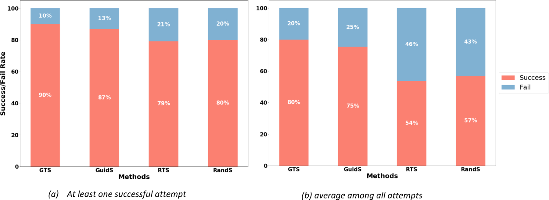
The rate at which each method successfully found a solution with a lower objective function value than that of the CG solution. Each attempt was limited to 1000 seconds. 3a) The percentages of test cases in which each method found a solution better than CG’s solution in at least 1 of their 5 attempts. 3b) The percentage of test cases in which each method found a solution better than CG’s solution, averaged over all 5 of their attempts to solve the problem.

The domain of the objective function value varied for different test-case scenarios, so we introduced the Distance measure to normalize the objective values of the four methods for further comparison with the CG solutions. The Distance measure is the difference between the objective function value of each method and that of CG, divided by the CG objective value ($Distance=\frac{C{G}_{obj}-metho{d}_{obj}}{C{G}_{obj}}\times 100$).

If a method finds a solution better than CG, the Distance measure will be positive; if a method does not find a solution better than CG, this value will be negative. This means that the method with the largest Distance measure found the solutions with the best quality—with objective values smaller than those of CG—more efficiently than CG, as the time was limited to 1000 seconds. Figure 4 shows the box plot of Distance measures for the GTS, GuidS, RTS, and RandS methods. As shown in this figure, the average Distance measure for the GTS method was 2.48, which was higher than for the other three methods: 1.76 for GuidS, 0.67 for RTS, and 0.81 for RandS.

Figure 4:

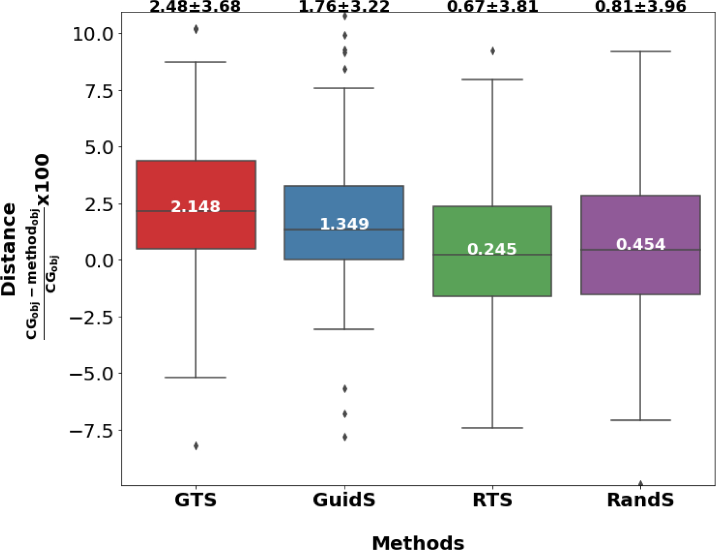
The Distance measure of the average of the best objective function value found by each method compared to CG’s solution. The value inside the box is the median, and the value at the top of each box-plot is the mean plus or minus standard deviation of the Distance measure.

For the computational time evaluation and comparison measures, we only considered the 102 test cases where all four methods found a better solution than CG within the 1000-second time limit. The box-plot of the best time needed to beat the CG solution is presented in Figure 5a. This represents the first time that a method found a solution better than CG’s solution within 1000 seconds across all five attempts. The box-plot of the average time to beat CG across all attempts to solve each test case is provided in Figure 5b. To measure the average time to beat CG, we considered all test cases and all attempts. The fastest method according to this measure was GTS, whose average time to beat CG was 51 seconds in the best case and 237 seconds across all cases. The second fastest method was RTS with average time of 55 seconds for the best case, while GuidS had the average time of 65 seconds for the best case, and RandS had the worst performance of 84 seconds. However, when the average time of all attempts were considered, GuidS beat CG in 268 seconds, RandS in seconds and RTS had the worst performance of 338 seconds on average.

Figure 5:

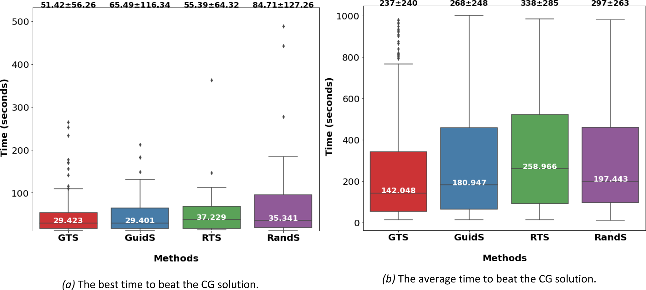
The computational time comparison between GTS, GuidS, RandS and RTS. a) The first time that each method beats a column generation solution. For this measure only successful scenarios are considered. Mean, standard deviation (at the top of each box as mean plus or minus standard deviation) and median (in the middle of the box) are calculated for each method.

Figure 6 shows the search rate for each methods, the search rate is calculated by dividing the total number of nodes in the search tree by its computational time. The number presented in this figure represents how many nodes are visited per minute for each method. As it is shown GTS has the highest rate of visiting nodes. We believe, the one by one selection of beams and storing the prediction data throughout the tree, can cause more efficient method to explore the tree, unlike GuidS, which needs to use model prediction at each node and may causes the occupation of extra time and space. Next method with highest rate is RandS. RandS can explore more nodes per minute, but this method does not save any history of previous tree traversal, so the computational resources are largely available for this method. However, this method is not guided and therefore not efficient, even with exploring more nodes on the tree, finding better solutions has no guaranty. Finally, the RTS method, and later GuidS, GuidS is the most computationally demanding method, due to the its frequent use of DNN for each node to be visited. GuidS does not save the history of a node and therefore needs to use the loaded DNN to predict the next fitness values of each nodes, while RTS does not need to load and use DNN, but save a history of the tree search traversal.

Figure 6:

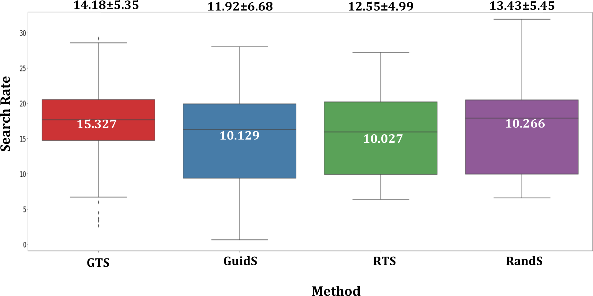
Search Rate for each methods, which is the total number of tree nodes divided by its computational time ( $\frac{\left|TreeNodes\right|}{Time\left(minute\right)}$) for each methods. To convert the total number of nodes for RandS which does not have a search tree, the total number of solutions are multiplied by 5.

To study the statistical significance of the differences between the performance of GTS and the other four methods (GuidS, RTS, RandS, and CG), we used a one-tailed paired sample t-test to compare the objective function values of each pair of methods, as well as the Distance measure. The null hypothesis is that the average objective function and Distance measures of all methods are the same. If we show the null hypothesis as GTS = GuidS = RandS = RTS = CG = 0, the alternative hypothesis can be described as GTS < GuidS < RandS < RTS < CG for the objective value parameters and GTS > GuidS > RandS > RTS > CG for the Distance measure. Ten paired sample t-tests were performed for objective function values and Distance measures. These statistics are presented in Table 1. The distributions of objective values and Distance measures are provided in appendix section VI. In Table 1, the values highlighted in red show that all pairings of CG, RTS, and RandS have p-values greater than 0.01 and thus, are not significantly different. In contrast, the average Distance and objective value measures of GuidS and GTS differ significantly from the other methods. These results show that GTS outperforms all other methods significantly and GuidS performs second best, as we expected.

Table 1:

One-tailed paired sample t-test to test the average objective function value and Distance measure for every pair of CG, GTS, GuidS, RTS, and RandS methods, with %99 confidence intervals. All values in red have p-values greater than 0.01.

	Objective Value		Distance ($\frac{\mathit{C}\mathit{G}-\mathit{o}\mathit{b}\mathit{j}}{\mathit{C}\mathit{G}}$)
Tested methods	t-statistic	p-value	t-statistic	p-value
CG vs GTS	6.267	2.54E-09	7.683	1.72E-12
CG vs GuidS	4.940	1.19E-06	6.393	1.37E-09
CG vs RTS	0.885	1.89E-01	2.014	2.30E-02
CG vs RandS	1.670	4.87E-02	2.340	1.04E-02
RandS vs RTS	−1.496	6.85E-02	1.096	1.38E-01
RandS vs GTS	6.826	1.53E-10	−11.843	1.18E-22
RandS vs GuidS	3.873	8.51E-05	−4.839	1.83E-06
RTS vs GTS	8.245	8.18E-14	−15.271	5.25E-31
RTS vs GuidS	5.257	2.95E-07	−5.832	2.08E-08
GuidS vs GTS	2.412	8.64E-03	−3.945	6.52E-05

PTV statistics, Paddick Conformity Index (CI_Paddick) and dose spillage (R₅₀) of plans generated by CG, GTS, GuidS, RTS, and RandS are presented in Table 2. Note that PTV D₂ is used to measure PTV D_max, as recommended by the ICRU Report 83[56]. The plans generated by all methods have very similar PTV coverage. CG plans have the highest CI_Paddick, followed by GTS and GuidS plans. CG and GuidS plans have the lowest dose spillage values, followed by GTS.

Table 2:

Mean ± standard deviation for PTV Statistics, Paddick Conformity Index (CI_Paddick), and High Dose Spillage (R₅₀) of the GTS, GuidS, RTS, RandS, and CG methods.

Method	PTV D98	PTV D99	PTV Dmax	PTV Homogeneity	CIPaddick	R50
GTS	0.977 ± 0.011	0.960 ± 0.019	1.070 ± 0.040	0.089 ± 0.045	0.874 ± 0.061	4.569 ± 0.994
GuidS	0.976 ± 0.012	0.960 ± 0.019	1.071 ± 0.040	0.089 ± 0.046	0.874 ± 0.068	4.487 ± 0.948
RTS	0.977 ± 0.011	0.959 ± 0.020	1.070 ± 0.039	0.088 ± 0.045	0.863 ± 0.085	4.714 ± 1.312
RandS	0.977 ± 0.012	0.960 ± 0.019	1.071 ± 0.040	0.089 ± 0.046	0.867 ± 0.070	4.673 ± 1.022
CG	0.977 ± 0.011	0.961 ± 0.020	1.072 ± 0.041	0.090 ± 0.046	0.884 ± 0.059	4.478 ± 0.963

The average and maximum doses received by each structure are provided in Table 3. These values reflect the fractional dose in plans generated by each method with the assumption that the prescription dose is one; e.g., if the prescription dose is 70 Gy, the average dose of 0.207 in the table means 14.47 Gy (0.207 × 70) in the prescribed plan. The minimum values in each row are shown in bold for easier interpretation. On average, plans generated by GTS have lower mean doses to OARs than the other methods, while plans generated by CG have the lowest maximum doses to OARs. GTS plans spare rectum and right femoral head better than the other methods. Although the average fractional dose to bladder by GTS plans (0.207) is higher than by CG plans (0.204), GTS plans have a lower maximum fractional dose to bladder (1.094) than CG plans (1.095). GuidS plans have the lowest average fractional dose to left femoral head (0.201), which is considerably lower than for RandS plans (0.212), which performed second best. As an example, Figure 7 shows the dose volumes and dose washes of plans generated by GTS and CG for one test case scenario.

Table 3:

The average and maximum fractional dose received by each structure in plans generated by GTS, GuidS, RTS, RandS, and, CG methods, where prescription dose is set to 1.

			Methods
	Structures	GTS	GuidS	RTS	RandS	CG
Mean Dose	PTV	1.039 ± 0.025	1.039 ± 0.025	1.038 ± 0.024	1.039 ± 0.025	1.040 ± 0.025
	Body	0.037 ± 0.012	0.037 ± 0.012	0.037 ± 0.012	0.037 ± 0.012	0.038 ± 0.013
	Bladder	0.207 ± 0.125	0.207 ± 0.122	0.207 ± 0.126	0.206 ± 0.122	0.204 ± 0.116
	Rectum	0.317 ± 0.109	0.321 ± 0.111	0.319 ± 0.110	0.322 ± 0.115	0.334 ± 0.116
	L-femoral	0.213 ± 0.105	0.201 ± 0.103	0.217 ± 0.115	0.212 ± 0.111	0.222 ± 0.112
	R-femoral	0.214 ± 0.101	0.221 ± 0.110	0.227 ± 0.124	0.224 ± 0.124	0.217 ± 0.109
Max Dose	PTV	1.113 ± 0.055	1.113 ± 0.055	1.113 ± 0.055	1.114 ± 0.057	1.116 ± 0.058
	Body	1.190 ± 0.131	1.195 ± 0.148	1.200 ± 0.147	1.199 ± 0.143	1.173 ± 0.130
	Bladder	1.094 ± 0.046	1.094 ± 0.048	1.096 ± 0.050	1.094 ± 0.045	1.095 ± 0.048
	Rectum	1.072 ± 0.045	1.071 ± 0.044	1.073 ± 0.045	1.074 ± 0.048	1.071 ± 0.040
	L-femoral	0.609 ± 0.193	0.596 ± 0.209	0.619 ± 0.215	0.609 ± 0.220	0.613 ± 0.193
	R-femoral	0.639 ± 0.242	0.650 ± 0.249	0.625 ± 0.236	0.628 ± 0.244	0.617 ± 0.245

Figure 7:

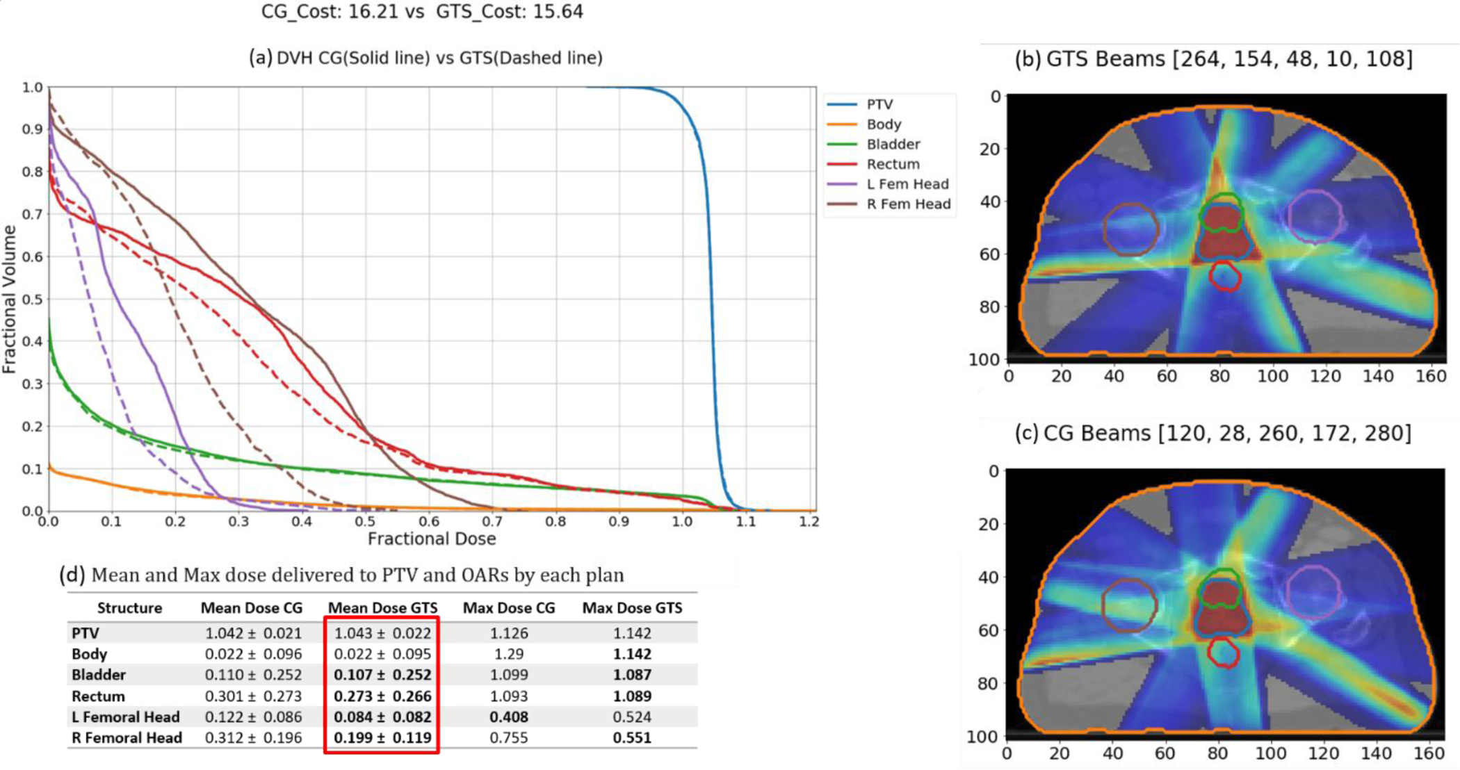
GTS-generated plan vs CG-generated plan. (a) DVH graph (GTS-generated plan(dashed) vs CG generated plan (solid).(b) Dosewash of GTS-generated plan.(c)Dosewash of CG-generated plan. (d) Mean and Maximum unite dose delivered to PTV and OARs by each plan.

IV. Discussion

In this research, we propose an efficient beam orientation optimization framework that can find a better solution than CG in a shorter amount of time by utilizing a reinforcement learning structure involving a supervised learning network, DNN, to guide Monte Carlo Tree Search to explore the beam orientation selection decision space.

Although CG is a powerful optimization tool, it is a greedy approach that is computationally expensive and time consuming, and it also may get stuck in a local optimum. This is particularly true for highly non-linear optimization problems with many local optima, such as BOO. In this work, we tried to improve upon CG via four different approaches: 1) Guided Tree Search (GTS), 2) Guided Search (GuidS), 3) Random Tree Seach (RTS), and 4) Random Search (RandS). Although the quality of solutions obtained using RandS, RTS and CG did not differ significantly, both RandS and RTS, which have no knowledge of the problem at the beginning of the search, found solutions better than CG in 50% of the test cases. This shows the high potential of improving upon the solution found by CG.

We saw that GTS and GuidS both performed better than the other methods, which we expected because both of these methods use prior knowledge (a trained DNN) to explore the solution space. GTS outperforms even GuidS on average, because GTS combines GuidS with RTS, which means that adding a search method to GuidS can improve the quality of the solution. But considering the insignificant difference between the performances of RTS and RandS, adding any search method to GuidS may result in better solutions, and the improvement may not be directly related to RTS. This issue will be studied in future research. The poor performance of RTS may also suggest that using a uniform tree search is too slow to converge to the optimal selection of beams.

GTS found solutions with better objective function values than the other methods, but the dose spillage metrics, specifically the average dose received by bladder in GTS plans, can be improved further. Considering the success of GTS in reducing the objective function and its potential for further improvement, we will continue exploring new methods and techniques to upgrade the quality of treatment planning with the help of artificial intelligence.

We should note that CG is a greedy and deterministic algorithm, so using CG on the same problem always results in the same solution. This is of a completely different nature from our search methods, so it may not be fair to compare its performance with the four search procedures, which, given infinite time and resources, can act as brute force approaches and guarantee finding the optimal solution. However, our main goal is to find the best possible solution for the BOO problem, and in this work, we try to see which search algorithms can find the best solutions the fastest. We expect to see search algorithms outperform greedy algorithms. The resulting objective function values showed us that GTS, GuidS, RTS, RandS, and CG all perform similarly. Plans generated by DNN solutions may not be superior to CG, but the DNN can mimic the CG algorithm very efficiently[49] and explore the search space successfully, as shown by GuidS and GTS, especially when compared to CG, which can easily exhaust computational resources and is very slow to find a single solution for a problem. CG’s good performance compared to RandS and RTS shows how powerful the CG method can be to find a solution, and the success of using DNN to explore the decision space represents the proper knowledge that can be achieved by learning from CG.

This work follows the feasibility study of using DNN[49], and is limited to the selection of five beam orientations, however it can be applied for selecting larger number of beam orientations as well, provided that the DNN (the guiding methods) is trained on cases with more than five beam orientations. Note that current DNN can be used to predict 6^th, 7^th, et. beams, but the prediction error is expected to be high, since it is not trained on such examples. CG needs to be used to create training examples with six or more number of beam orientations, and that requires more computational memory and time. Furthermore, the size of the tree will grow exponentially by selecting more beam orientations, which increases the size of each branch, and requires more space and time to be processed, and a time limit of 1000 seconds may not be an applicable. Moreover, we study coplanar BOO problem, which has limited number of potential beam orientations to begin with (180 beams with 2° seperation), but for non-coplanar BOO, the number of potential beams to select from may be a lot larger, for example 1162 in 4π non-coplanar beam selection[57]. Processing larger number of potential beam orientations requires even more computational time and space, although it may affect the training time and the architecture of the DNN, the structure of the tree-search proposed here can still be used with no change, but the depth of the tree will be highly affected by the size of the selected beam orientations. Hence, the GTS is suitable for selection of limited number of beams, however for selection of larger set of beam orientations, more research is required.

Finally, GTS is a problem-specific search method that must be applied to each test case separately. To use the knowledge that we can get from the GTS performance, more advanced reinforcement algorithms can be trained to create a single general knowledge-based method that is not only very powerful in finding the best possible solutions, but also very fast in doing so. The advanced reinforcement learning method can then be easily applied to more sophisticated and challenging problems, such as proton and 4π radiation therapy. For future studies, we are working to develop a smart, fast and powerful tool to apply to these problems.

V. Conclusion

In this study, we proposed a Monte Carlo guided tree search (GTS) to show finding a solution with a better objective function compared to CG, in a reasonable amount of time is feasible. GTS uses a pre-trained DNN to guide the Monte Carlo Tree Search. DNN generates the beams’ fitness values for nodes in the decision tree, where each node represents a set of selected beams. GTS continues to explore the decision tree for 1000 seconds. Along with GTS, we tested three other approaches: GuidS, which also uses a pre-trained DNN to select beams iteratively but does not update the probability distribution of beams during the search process; RTS, which is a simple tree search algorithm that starts by randomly sampling from a uniform distribution of beam orientations for each node and continues to update beams’ probability distribution based on the tree search approach presented for GTS; and RandS, which randomly selects beams—this is the most trivial and simple approach.

VII. Appendix

Although statistically, with 130 test cases, we can assume that our metrics approximately follow a normal distribution, the graphs in Figure 7a suggest that this assumption may not be practical. Because of this, we introduced Distance measures to normalize our metrics. The probability distribution and cumulative probability mass function of Distance measures are presented in Figure 7b. By this graph, we can verify that this measure approximately normally distributed with a similar standard deviation.

Figure 7:

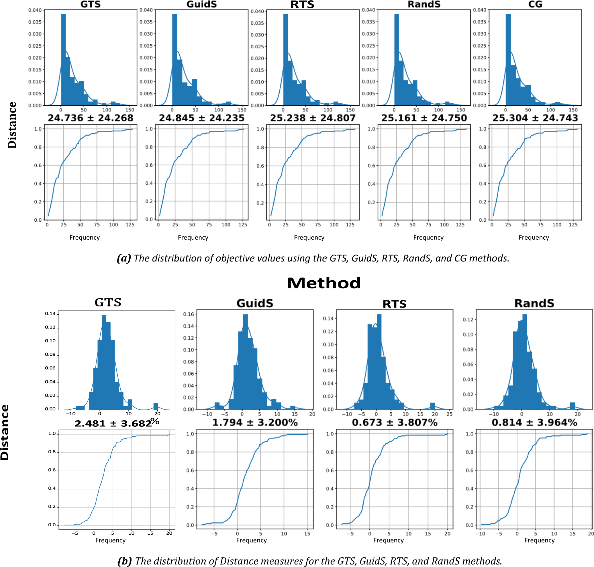
The distribution of objective values and distance to CG objective values. (a) top row shows the distribution of objective values for each method, bottom row shows the distribution of the cumulative objective values for each method. (b) top row shows the distribution of Distance measure for each method, while its bottom rows shows the cumulative distribution of Distance measure. All graphs share the x and y labels, x label is distance while the y label is frequency.

References

- 1.Baskar R, et al. , Cancer and radiation therapy: current advances and future directions. International journal of medical sciences, 2012. 9(3): p. 193–199. [DOI] [PMC free article] [PubMed] [Google Scholar]
- 2.Taylor A and Powell MEB, Intensity-modulated radiotherapy--what is it? Cancer imaging : the official publication of the International Cancer Imaging Society, 2004. 4(2): p. 68–73. [DOI] [PMC free article] [PubMed] [Google Scholar]
- 3.Breedveld S, et al. , iCycle: Integrated, multicriterial beam angle, and profile optimization for generation of coplanar and noncoplanar IMRT plans. Medical physics, 2012. 39(2): p. 951–963. [DOI] [PubMed] [Google Scholar]
- 4.Ehrgott M, Holder A, and Reese J, Beam selection in radiotherapy design. Linear Algebra and Its Applications, 2008. 428(5–6): p. 1272–1312. [Google Scholar]
- 5.Bangert M and Oelfke U, Spherical cluster analysis for beam angle optimization in intensity-modulated radiation therapy treatment planning. Physics in Medicine & Biology, 2010. 55(19): p. 6023. [DOI] [PubMed] [Google Scholar]
- 6.Cabrera G,G, et al. , A metaheuristic approach to solve the multiobjective beam angle optimization problem in intensity-modulated radiation therapy. International Transactions in Operational Research, 2018. 25(1): p. 243–268. [Google Scholar]
- 7.Bortfeld T and Schlegel W, Optimization of beam orientations in radiation therapy: some theoretical considerations. Physics in Medicine & Biology, 1993. 38(2): p. 291. [DOI] [PubMed] [Google Scholar]
- 8.Rowbottom CG, Webb S, and Oldham M, Beam-orientation customization using an artificial neural network. Physics in Medicine & Biology, 1999. 44(9): p. 2251. [DOI] [PubMed] [Google Scholar]
- 9.Pugachev A, et al. , Role of beam orientation optimization in intensity-modulated radiation therapy. International Journal of Radiation Oncology* Biology* Physics, 2001. 50(2): p. 551–560. [DOI] [PubMed] [Google Scholar]
- 10.Djajaputra D, et al. , Algorithm and performance of a clinical IMRT beam-angle optimization system. Physics in Medicine & Biology, 2003. 48(19): p. 3191. [DOI] [PubMed] [Google Scholar]
- 11.Yongjie L, Jonathan Y, and Dezhong Y, Automatic beam angle selection in IMRT planning using genetic algorithm. Physics in Medicine & Biology, 2004. 49(10): p. 1915. [DOI] [PubMed] [Google Scholar]
- 12.Li Y, et al. , A particle swarm optimization algorithm for beam angle selection in intensity-modulated radiotherapy planning. Physics in Medicine & Biology, 2005. 50(15): p. 3491. [DOI] [PubMed] [Google Scholar]
- 13.Romeijn HE, et al. , A column generation approach to radiation therapy treatment planning using aperture modulation. SIAM Journal on Optimization, 2005. 15(3): p. 838–862. [Google Scholar]
- 14.Schreibmann E and Xing L, Dose–volume based ranking of incident beam direction and its utility in facilitating IMRT beam placement. International Journal of Radiation Oncology*Biology*Physics, 2005. 63(2): p. 584–593. [DOI] [PubMed] [Google Scholar]
- 15.Aleman DM, et al. , Neighborhood search approaches to beam orientation optimization in intensity modulated radiation therapy treatment planning. Journal of Global Optimization, 2008. 42(4): p. 587–607. [Google Scholar]
- 16.Lim GJ, Choi J, and Mohan R, Iterative solution methods for beam angle and fluence map optimization in intensity modulated radiation therapy planning. OR Spectrum, 2008. 30(2): p. 289–309. [Google Scholar]
- 17.Breedveld S, Storchi P, and Heijmen B, The equivalence of multi-criteria methods for radiotherapy plan optimization. Physics in Medicine & Biology, 2009. 54(23): p. 7199. [DOI] [PubMed] [Google Scholar]
- 18.Lim GJ, Holder A, and Reese J. A clustering approach for optimizing beam angles in IMRT planning. in IIE Annual Conference. 2009. [Google Scholar]
- 19.Craft D and Monz M, Simultaneous navigation of multiple Pareto surfaces, with an application to multicriteria IMRT planning with multiple beam angle configurations. Medical Physics, 2010. 37(2): p. 736–741. [DOI] [PMC free article] [PubMed] [Google Scholar]
- 20.Rocha H, et al. , Beam angle optimization for intensity-modulated radiation therapy using a guided pattern search method, in Physics in Medicine and Biology. 2013. p. 2939–2953. [DOI] [PubMed] [Google Scholar]
- 21.Yuan L, et al. , Standardized beam bouquets for lung IMRT planning, in Physics in Medicine and Biology. 2015, Institute of Physics Publishing. p. 1831–1843. [DOI] [PMC free article] [PubMed] [Google Scholar]
- 22.Amit G, et al. , Automatic learning-based beam angle selection for thoracic IMRT. Medical Physics, 2015. 42(4): p. 1992–2005. [DOI] [PubMed] [Google Scholar]
- 23.Liu H, Dong P, and Xing L, A new sparse optimization scheme for simultaneous beam angle and fluence map optimization in radiotherapy planning. Physics in Medicine & Biology, 2017. 62(16): p. 6428. [DOI] [PubMed] [Google Scholar]
- 24.Cabrera-Guerrero G, et al. , Comparing Local Search Algorithms for the Beam Angles Selection in Radiotherapy. IEEE Access, 2018. 6: p. 23701–23710. [Google Scholar]
- 25.Rocha H, et al. Comparison of Combinatorial and Continuous Frameworks for the Beam Angle Optimization Problem in IMRT. in International Conference on Computational Science and Its Applications. 2018. Springer. [Google Scholar]
- 26.O’Connor D, et al. , Fraction-variant beam orientation optimization for non-coplanar IMRT. Physics in Medicine & Biology, 2018. 63(4): p. 045015. [DOI] [PMC free article] [PubMed] [Google Scholar]
- 27.Cabrera-Guerrero G, et al. , Pareto local search algorithms for the multi-objective beam angle optimisation problem. Journal of Heuristics, 2018. 24(2): p. 205–238. [Google Scholar]
- 28.Ramar N, et al. , Objective function based ranking method for selection of optimal beam angles in IMRT. Physica Medica, 2020. 69: p. 44–51. [DOI] [PubMed] [Google Scholar]
- 29.Ventura T, et al. , Comparison of two beam angular optimization algorithms guided by automated multicriterial IMRT. Physica Medica, 2019. 64: p. 210–221. [DOI] [PubMed] [Google Scholar]
- 30.Potrebko PS, et al. , Improving intensity-modulated radiation therapy using the anatomic beam orientation optimization algorithm. Medical Physics, 2008. 35(5): p. 2170–2179. [DOI] [PubMed] [Google Scholar]
- 31.Jorge L, et al. , Non-coplanar automatic beam orientation selection in cranial IMRT: a practical methodology. Physics in Medicine & Biology, 2009. 54(5): p. 1337. [DOI] [PubMed] [Google Scholar]
- 32.Yu VY, et al. , A Prospective 4π Radiation Therapy Clinical Study in Recurrent High-Grade Glioma Patients. International Journal of Radiation Oncology*Biology*Physics, 2018. 101(1): p. 144–151. [DOI] [PubMed] [Google Scholar]
- 33.Yarmand H and Craft D, Effective heuristics for beam angle optimization in radiation therapy. SIMULATION, 2013: p. 0037549718761108. [Google Scholar]
- 34.Lulin Y, et al. , Lung IMRT planning with automatic determination of beam angle configurations. Physics in Medicine & Biology, 2018. 63(13): p. 135024. [DOI] [PMC free article] [PubMed] [Google Scholar]
- 35.Rocha H, et al. , Beam angle optimization in IMRT: are we really optimizing what matters? International Transactions in Operational Research, 2018. 0(0). [Google Scholar]
- 36.Bedford JL, et al. , Beam selection for stereotactic ablative radiotherapy using Cyberknife with multileaf collimation, in Medical Engineering and Physics. 2019, Elsevier. p. 28–36. [DOI] [PMC free article] [PubMed] [Google Scholar]
- 37.Ventura T, et al. , Comparison of two beam angular optimization algorithms guided by automated multicriterial IMRT, in Physica Medica. 2019, Elsevier. p. 210–221. [DOI] [PubMed] [Google Scholar]
- 38.Haseai S, et al. , Similar-cases-based planning approaches with beam angle optimizations using water equivalent path length for lung stereotactic body radiation therapy. Radiological Physics and Technology, 2020. 13(2): p. 119–127. [DOI] [PubMed] [Google Scholar]
- 39.Oelfke U and Bortfeld T, Inverse planning for photon and proton beams. Medical Dosimetry, 2001. 26(2): p. 113–124. [DOI] [PubMed] [Google Scholar]
- 40.Gu W, et al. , Integrated beam orientation and scanning-spot optimization in intensity-modulated proton therapy for brain and unilateral head and neck tumors. Medical physics, 2018. 45(4): p. 1338–1350. [DOI] [PMC free article] [PubMed] [Google Scholar]
- 41.Shirato H, et al. , Selection of external beam radiotherapy approaches for precise and accurate cancer treatment, in Journal of Radiation Research. 2018, Oxford University Press. p. i2–i10. [DOI] [PMC free article] [PubMed] [Google Scholar]
- 42.Gu W, et al. , Robust Beam Orientation Optimization for Intensity-Modulated Proton Therapy, in Medical Physics. 2019, John Wiley & Sons, Ltd. p. mp.13641. [DOI] [PMC free article] [PubMed] [Google Scholar]
- 43.Taasti VT, et al. , Automating proton treatment planning with beam angle selection using Bayesian optimization. Medical Physics, 2020. 47(8): p. 3286–3296. [DOI] [PMC free article] [PubMed] [Google Scholar]
- 44.Gu W, et al. , Fraction-variant beam orientation optimization for intensity-modulated proton therapy. Medical Physics, 2020. 47(9): p. 3826–3834. [DOI] [PMC free article] [PubMed] [Google Scholar]
- 45.Azizi-Sultan AS, Optimization of Beam Orientations in Intensity Modulated Radiation Therapy. 2006.
- 46.Dong P, et al. , 4π non-coplanar liver SBRT: a novel delivery technique. International Journal of Radiation Oncology* Biology* Physics, 2013. 85(5): p. 1360–1366. [DOI] [PubMed] [Google Scholar]
- 47.Rwigema JCM, et al. , 4π noncoplanar stereotactic body radiation therapy for head-and-neck cancer: Potential to improve tumor control and late toxicity, in International Journal of Radiation Oncology Biology Physics. 2015, Elsevier Inc. p. 401–409. [DOI] [PubMed] [Google Scholar]
- 48.Nguyen D, et al. , Computerized triplet beam orientation optimization for MRI-guided Co-60 radiotherapy. Medical physics, 2016. 43(10): p. 5667–5675. [DOI] [PMC free article] [PubMed] [Google Scholar]
- 49.Sadeghnejad Barkousaraie A, et al. , A Fast Deep Learning Approach for Beam Orientation Optimization for Prostate Cancer Treated with Intensity Modulated Radiation Therapy, in Medical Physics. 2019, Wiley. [DOI] [PMC free article] [PubMed] [Google Scholar]
- 50.Chambolle A and Pock T, A first-order primal-dual algorithm for convex problems with applications to imaging. Journal of mathematical imaging and vision, 2011. 40(1): p. 120–145. [Google Scholar]
- 51.Kuhn HW and Tucker AW. Nonlinear Programming. in Proceedings of the Second Berkeley Symposium on Mathematical Statistics and Probability. Ed. Neyman J. Berkeley: Univ. of California Press. 1951. University of California Press, Berkeley [Google Scholar]
- 52.Karush W, Minima of functions of several variables with inequalities as side conditions, in Traces and Emergence of Nonlinear Programming. 2014, Springer; Basel. p. 217–245. [Google Scholar]
- 53.Browne CB, et al. , A survey of Monte Carlo tree search methods, in IEEE Transactions on Computational Intelligence and AI in Games. 2012. p. 1–43. [Google Scholar]
- 54.Riet A.v.t., et al. , A conformation number to quantify the degree of conformality in brachytherapy and external beam irradiation: Application to the prostate. International Journal of Radiation Oncology*Biology*Physics, 1997. 37(3): p. 731–736. [DOI] [PubMed] [Google Scholar]
- 55.Paddick I, A simple scoring ratio to index the conformity of radiosurgical treatment plans. 2000. 93(supplement_3): p. 219. [DOI] [PubMed] [Google Scholar]
- 56.Hodapp N, The ICRU Report No. 83: Prescribing, recording and reporting photon-beam intensity-modulated radiation therapy (IMRT), in Strahlentherapie und Onkologie. 2012, Springer. p. 97–99. [DOI] [PubMed] [Google Scholar]
- 57.Nguyen D, et al. , Integral dose investigation of non-coplanar treatment beam geometries in radiotherapy. Medical Physics, 2014. 41(1): p. 011905. [DOI] [PubMed] [Google Scholar]