Machine learning in postgenomic biology and personalized medicine

Abstract

In recent years Artificial Intelligence in the form of machine learning has been revolutionizing biology, biomedical sciences, and gene-based agricultural technology capabilities. Massive data generated in biological sciences by rapid and deep gene sequencing and protein or other molecular structure determination, on the one hand, requires data analysis capabilities using machine learning that are distinctly different from classical statistical methods; on the other, these large datasets are enabling the adoption of novel data-intensive machine learning algorithms for the solution of biological problems that until recently had relied on mechanistic model-based approaches that are computationally expensive. This review provides a bird’s eye view of the applications of machine learning in post-genomic biology. Attempt is also made to indicate as far as possible the areas of research that are poised to make further impacts in these areas, including the importance of explainable artificial intelligence (XAI) in human health. Further contributions of machine learning are expected to transform medicine, public health, agricultural technology, as well as to provide invaluable gene-based guidance for the management of complex environments in this age of global warming.

Graphical Abstract

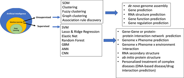
Broad classification of machine learning methods and their well-known applications to postgenomic biology. Only a few selected example applications are listed. Emerging fields of metagenomics and genomics-guided ecological engineering, not mentioned here, will increasingly see applications of machine learning in the future. Abbreviations: SOM, self-organized map; SVM, support vector machine; GBM, gradient boosting machine; ANN, artificial neural network; CNN, convolutional neural network.

1. Introduction

Since the advent of high speed computing and neural networks in the 1990s, artificial intelligence (AI) has found numerous inroads into genomics-inspired biological and medical sciences. A recent excitement in this field concerns the ab initio folding of a protein using deep learning, ushering a new era of computationally enabled molecular biology. In this review, we will briefly sketch the history of AI in genomics, followed by a more general review of various AI algorithms currently in use in molecular biology, genomics and medicine. Due to lack of expertise, the author will refrain from discussing the enormously successful applications of AI on biological and biomedical imaging. The impact of AI on biomedical applications that have not been directly influenced by genomics will also not be addressed in this review.

A few words of explanations are needed in the beginning. A genome is the collection of all gene sequences (in terms of, most frequently, DNA sequence, but sometimes also RNA sequence) of an organism. ‘Post-genomic’ refers to the world after the year 2000, when the entire human genome was sequenced twice over, and the new science of ‘genomics’—the quantitative model instructed analysis of the effects of genes on organisms—was born. Genomics today encompasses problems and questions not just of those related to human beings but also of all organisms.

To the students of computer science AI and machine learning (ML) do not require definitions but for those readers who might be biologists or students of medicine we should emphasize a critical distinction between the two. AI is a general term that encapsulates the idea that algorithmic computation can analyze large datasets to determine multivariate relationships among data objects. ML on the other hand is a more specific discipline within AI that concerns itself to learning rules from previous data to predict future data. ML has two main approaches, unsupervised and supervised ML. The former is an approach to classify and/or cluster the data into distinct or overlapping groups based on similarities of patterns of variables within the data using arbitrary mathematical rules that are specified by a human operator. In the supervised approach, the data consist of a set of input variables and output variables (nominal or quantitative), where depending on the characteristics of the output variable it is a classification or regression problem. Supervised ML requires previous data and certain instances in which subsets of data points are preassigned to specific classes. The algorithm then trains an internal model; using the trained model, the algorithm predicts the assignment of new data to classes or predicts the values of the dependent variable given future data on the predictor variables. In general, this method iteratively refines the rules of classification or regression (see later). Deep learning is the special case of ML wherein neural networks of many layers are employed. A few example areas of application of unsupervised and supervised ML in post-genomic biology are provided in Graphical Abstract.

In this brief review, we will define for the lay person the fundamental concepts of machine learning, their applications to a few well-defined biological problems that had been intractable until ML methods were applied, describe the biological basis of personalized medicine, and highlight those specific areas in post-genomic biomedical sciences where ML are likely to impact in the future. The importance of “explainable artificial intelligence” for post-genomic biology will be emphasized. This review is primarily directed at students—not to present an exhaustive overview of the current literature but to attract their attention to future challenges in the biomedical sciences where ML should play an increasingly dominant role. For a health and biomedical discipline-specific review of ML applications, the reader is referred to an excellent recent review (Williams et al. 2018).

2. The need for ML in post-genomic biology

The paradigm of biology is that genes store information in an array (or arrays) of base pairs of nucleic acids (DNA or RNA), which are then “expressed” in terms of mRNA or protein sequences. Proteins (and sometimes RNA) embody the information in terms of their three dimensional structures. Structure determines the physical interaction of proteins with other proteins, RNA, DNA, or other molecules, such as small molecule chemicals (also called metabolites) as well as drugs or drug-like molecules and pathogenic organisms.

Insofar as basic biology is concerned, ML has been successfully applied to predicting the boundaries of genes and non-genic regions on seemingly monotonous tracks of DNA (or RNA) base sequences of the genome, to classify or group genes into families of related genes by dint of numerous properties, to assign function to novel genes, to classify and assign structural and functional domains to regions of RNA and protein sequences by similarities and physical properties, to predict interaction partners of proteins (in terms of other proteins or other molecules such as DNA or RNA or small molecules) (Fig. 1). ML has also been relatively successful in enabling numerous technological feats needed for genome centered biology, such as the assembly of complex genomes with many repeated sequences from long and short reads of DNA sequences, including de novo genome assemblies, ab initio protein folding prediction, and the prediction of interaction partners of proteins or other macromolecules. Emerging areas of application where ML will increasingly play important role are the elucidation of complex gene regulatory networks, the behavior of such networks under changing conditions, the prediction of disease phenotypes (intensity, onset time, and/or prognostic profile) of patients given their genetic profiles, and population level complex phenotypic prediction among communities of organisms (see additional recent reviews on these subjects: (Huang et al. 2018; Williams et al. 2018; Hessler and Baringhaus 2018; Dey et al. 2019)). For deeper insights into the biological principles that drive these applications, the reader is referred to (Raval, Alpan and Ray, Animesh 2013).

Figure 1.

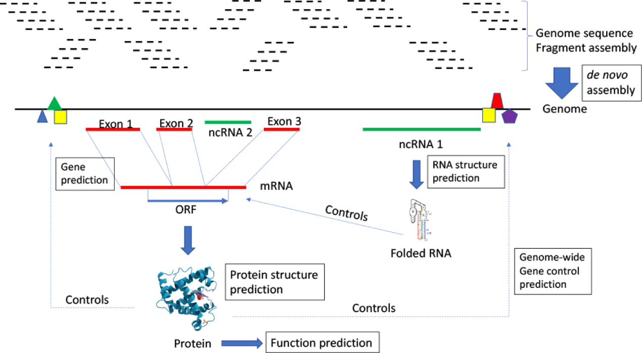
A bird’s eye view of challenging post-genomic biology where machine learning has been successful. Main areas of application are boxed. Most future progress however is expected to occur in “function prediction”, which involves modeling multicellular and multi-community interactions that span scales of distance (from sub-nanometer to meter) and time (from microseconds to evolutionary/geological timescales).

3. Machine Learning in Personalized Medicine

Humans have traveled the earth for the past ~250,000 years in waves of migration followed by geographical isolation and subsequent admixture of gene pools. Mutations spontaneously arise a frequency of ~10⁻⁹–10⁻⁸ per DNA nucleotide base per generation, as a result of which the haploid human genomic sequences of 3 × 10⁹ base pairs suffer on average ~1 mutation per generation, producing ~2 mutations per diploid individual. 6 billion humans currently inhabiting the earth therefore has about 12 × 10⁹ new mutations in this generation alone. Since one can estimate at least 5,000–10,000 generations since the speciation of modern man, with an estimated cumulative total 1.17 × 10¹¹ humans born on the earth, there have been the opportunity for ~2 × 10¹⁵ spontaneous DNA mutations. Many such mutations however were lethal or selectively disadvantageous, therefore were selected out; most were likely neutral and could have been lost due to genetic drift. Some would be extinguished naturally because the bearers of such mutations did not pass them on. Nonetheless, numerous genetic variants due to past mutational events are expected to occur in human populations; indeed, at the time of writing the database of single nucleotide variants (dbSNP: https://www.ncbi.nlm.nih.gov/snp/) for humans reports >9 × 10⁸ unique variants. Many of the rarer variants are known to be associated with defined human disorders because of their large phenotypic effects, and some of these variants have disproportionately high representation in the current human gene pools (Keinan and Clark 2012). However, most have no or mild effects on human biology but it is thought that in combination these multiple variants, each with mild effect, may explain individual variations to disease propensity (Matullo et al. 2013). The effort to decipher individual patient’s disease susceptibility or response to treatment on the basis of DNA sequence variations is known as personal genomics (Rehm 2017) (Fig. 2). Since the advent of low-cost DNA sequencing, personal genomics has become a reality for the treatment of certain diseases such as cancer, where increasingly individualized treatments are designed by teams of physicians and scientists guided by DNA sequencing of tumor and healthy cells of the patients. The challenge is to decipher the matrix of gene-variant x disease-condition for an individual (the relations among input variables) and then to map the matrix to a course of treatment optimized to reduce disease outcomes—a large nonlinear optimization problem that takes incomplete and noisy input variables and their relations to produce a “fuzzy” output variable that tries to capture the treatment parameters. The problem is also difficult because historical population structures (e.g., population bottlenecks, migration) and natural selection leaves signatures in the genome in terms of the distortion of the frequencies of gene variations from those estimable from equilibrium populations structures. These signatures are difficult to distinguish from those based on association with diseases, as one relevant objective.

Figure 2.

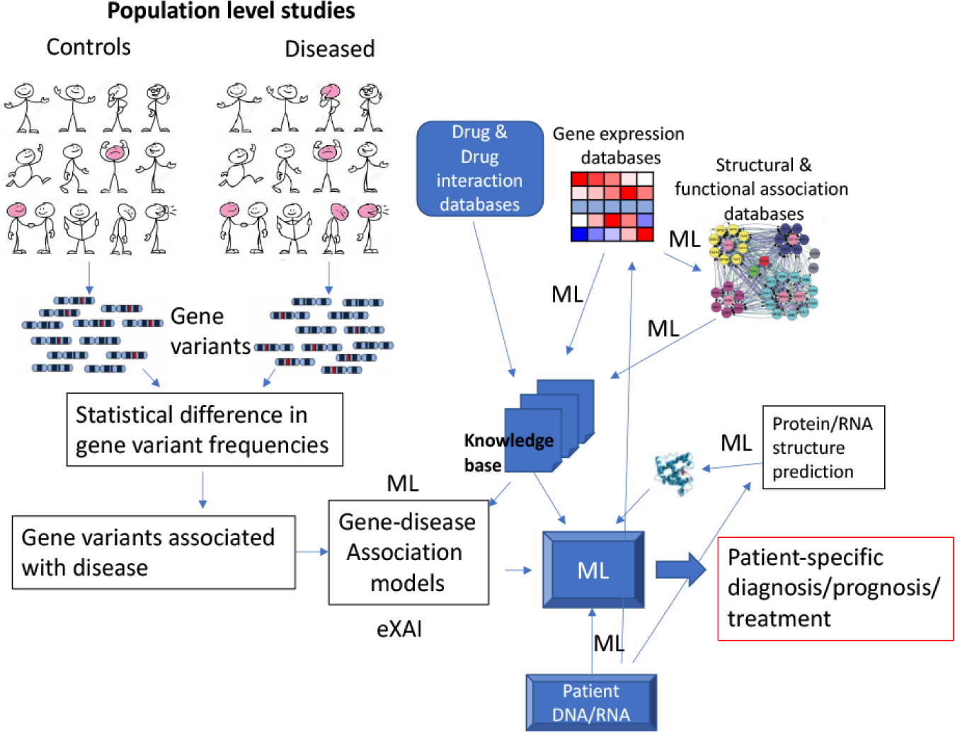
A broad overview of personalized medicine challenges for machine learning. Modeling population fine structures of genetic variants (colored in purple) to disease causation, especially for complex diseases of strong multi-genic and environmental influences, is an open challenge. Patient-specific diagnosis or prognostic models must solve the ‘black-box’ nature of deep learning.

The science of personal genomics is in its infancy and is mostly at the stage of research except in rare special cases, because of incomplete knowledge and understanding as well as computational challenges of very large datasets with high noise (Dudley and Karczewski 2013). Machine learning, especially deep learning, is thought to be ideally suited to accelerate the pace of progress in this field. And yet the field can make impact only if there is sufficient attention placed on “understanding” how the inputs and the outputs are causally related, which is often ignored in “black-box” paradigms of conventional machine-learning.

4. Two principles of Machine Learning: Regression and Classification

In classical statistics, one is generally trying to determine as accurately as possible what the output variables are when given a specific model (or a function) and a set of observable data providing the values of input variables. In brief,

$$y\leftarrow f\left(x\right)$$

Where the function f( ) and the input variable or observation x are given, and one is asked to compute y or map x to y.

In ML the problem is reversed. Given a set of input observations or data d^obs and a set of discriminatory variables v, the task is to infer a function or a model M( ), such that,

$$\mathit{M}\left(\mathit{v}\right)\to {\mathit{d}}^{obs}$$

In this latter problem, the model M( ) or the mapping function, which is a mathematical abstraction or a logical relationship, is unknown, and therefore it needs to be inferred—this activity is termed ‘model selection’. Moreover, the set of discriminatory variables v also needs to be defined from a subset of the real number space—this latter task is called ‘feature selection’. The process of model inference is made more and more accurate, while avoiding model overfitting, through training or learning from a subset (the training set) of d^obs. The trained model is then validated on another subset of d^obs which were not used in training (the test set), to assess the sensitivity and the specificity of the fit and to estimate the extent of model overfitting. The model is then ready for applying to additional data that might not have existed before. Note that the model can be iteratively made more and more accurate as new observations are made.

It might be obvious to the insightful reader that what we have described above is a regression problem. In classical regression, a function is deduced using a chosen mathematical model (e.g., the principle of least square) to estimate the best parameters that fit the observed data. The concept holds for high-dimensional and nonlinear regression models too. All ML algorithms are fundamentally regression algorithms. Whereas in classical regression the specific algorithm is deliberately defined prior to parameter estimation, in ML the regression algorithm is not explicitly defined. Regression takes as input the variables in the real number space and produces outputs that are also in the real number space. This holds true for both continuous and discrete or categorical variables, as in logistic regression, where discrete variables are converted to continuous probabilities over a particular probability distribution.

Imagine, on the other hand, that the output variables are discrete. In this case the model M( ) is no longer a conventional regression model, but is a “classification” model. In other words, an ML classifier is a model that allows the partitioning of the observed data into two or more classes or groups, providing a grouping of the data with associated probability values for such a grouping. As a special case, however, a regression model can be constrained to become a classification model in which the outputs are binned into discrete classes. Thus, all ML models can be thought of as regression models with or without constraints.

One of the most important problems in ML is the choice of the features or input variables (Guyon and Elisseeff 2003). A judicious selection of features vectors, and in many cases the engineering of feature vectors from high dimensional datasets, is considered fundamental to a successful model building. Feature selection has three main objectives: improving the performance of the predictor variables, providing faster and more cost-effective predictors from the large datasets, and providing a better understanding of the underlying process that generated the data (also a goal of “explainable AI”). Unlike in many data engineering applications, however, feature selection (such as choosing the important predictor variables and eliminating the noisy ones) rather than “feature engineering” has so far played a more important role in genomics because feature vectors are generally selected on the basis of prevailing biological or physical knowledge-base of the analysts. Feature engineering, such as vectors obtained from dimensionality reduction of input variables, or a nonlinear combination of multiple input variables, have generally been avoided in genomics applications because of difficulties with interpretability. Thus, interpretability takes precedence over the accuracy of prediction in genomics applications. Nonetheless, feature engineering, coupled with efforts to explain the variables, are likely to be increasingly important in future genomics research.

5. Unsupervised Machine Learning

Unsupervised ML (Graphical Abstract) is the class of ML classification methods that does not require previous examples of the classes, but constitute methods for exploring the data for the presence of similar groups of variables. Frequently used methods for data exploration to probe the presence of regularity or patterns in the data, such as Principal Component Analysis, will not be discussed here because these are not strictly ML methods. Some of the earliest uses of ML in biological research was in the form of unsupervised neural network and various clustering methods in grouping genes on the basis of similarities in their respective mRNA expression levels under different experimental or physiological conditions, when such highly parallel experimental measurements became feasible genome-wide for the first time in the late 1990s. An early example is the application of Self Organized Map or SOM (Kohonen 1990) to classify large groups of genes by similarities of their expression patterns (Tamayo et al. 1999). The concept of SOM is interesting not only because of its historical importance in early post-genomic biology, it also helps succinctly illustrate the principles of unsupervised ML.

5.1. SOM

Here the specific biological problem to be solved is as follows. Large groups of genes (about a thousand in a bacterium, about five to ten thousand in a fungus, about 15–20 thousand in insects or other invertebrates, about 22,000 in human and related apes, and over 30,000 in some plants) make messenger RNA (mRNA), which encode proteins, in response to different conditions that might change over time. The expression changes are changes in the amount or concentration (commonly referred to as ‘levels’ or ‘expression levels’) and values are in the real number space. For a biologist, it is important to be able to identify groups of genes whose expression level changes vary together or are correlated in some ways. As always in biology, in the absence of direct observation we make a simplifying hypothesis—here the hypothesis is that similarities in mRNA expression level changes are related to similarities in gene function—which may or may not be true. But the first objective is to classify groups of genes by similarities or differences in their expression level changes.

In SOM, we specify the number of clusters or groups arbitrarily (which is then varied for consistency), and also specify a topology—a 2-dimensional grid that provides a geometric relationship among the clusters (Tamayo et al. 1999). The algorithm learns from the data and finds the transformation rules that measures the optimal distances among the clusters—which clusters are near of far from one another. The SOM algorithm then learns a mapping function from the high dimensional space of the data points into the 2-dimensional grid. There is one point for each cluster on the grid (Fig. 3). Suppose we have a m × n grid with each grid point associated with a cluster of gene expression changes of means, μ_1,1 … μ_m,n. The SOM algorithm moves the cluster means around the high dimensions maintaining the topology specified by the 2-dimensional grid, and a data point is incorporated into the cluster with the closest mean. This process leads to the effect that nearby data points (i.e., genes with similar gene expression change values) tend to map to nearby grid points or clusters. While this is a rather geometrically visual way to classify datapoints, it is unclear what topologies in gene expression changes is an ideal descriptor of the biological reality—why a 2-dimensional grid and not a 3-dimensional grid? Moreover, the number of specified clusters must be specified arbitrarily, often determined by the analyst’s intuition, which injects a degree of subjectivity into model evaluation. Moreover, the time complexity of SOM does not scale well: T = O(S²), where T is the computational time and S is the size of the sample (Roussinov and Chen 1998). Direct head-to-head comparison was held between a SOM classifier and a Support Vector Machine classifier (see later) in distinguishing between small molecules that are either inhibitors or decoys of a human signal-transduction receptor important in cancer (Epidermal Growth Factor Receptor or EGFR) using the same feature vectors (Kong et al. 2016). These results showed that the two classifiers performed nearly equally well, though SOM was surpassed slightly in prediction accuracy. Recently, SOM has been incorporated within deep learning algorithms for teaching human emotions to robots (Churamani et al. 2017); its applications to discovering intrinsic patterns within massive post-genomic data sets, and to imaging of single cell phenotypes during drug-screening, remain under-explored. This latter aspect of SOM will be examined in a section on Deep Learning.

Figure 3.

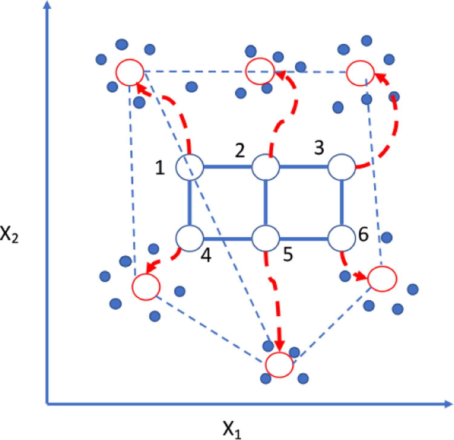
A cartoon diagram of Self Organized Map (SOM). Open circles represent an n x m dimensional grid. A neural network algorithm allows gradual mapping of the datasets (solid circles) according to the centroids that minimize a distance metric from their nearest neighbors; the emergent paths of the grid points are diagrammatized by the curved arrows. X₁ and X₂ are variables that describe the data. (Redrawn after (Tamayo et al., 1999))

5.2. Clustering

More frequently, standard methods of classification in genomics style of data analysis have been the K-means clustering and hierarchical clustering. In K-means clustering begins with an arbitrary number of k clusters, chosen intuitively; the algorithm then randomly assigns the data points to the clusters, calculates a centroid for each of the k clusters, calculates the distance (using a specified distance metric) of each data point to the k centroids followed by reassigning the data points to the closest centroid. The process is continued iteratively until cluster assignments are stable. Finally, each data point is assigned to a unique cluster such that no two clusters have the same gene.

In hierarchical clustering (Fig. 4A), a similarity metric is computed for the objects to be clustered (here, say, the log-transformed expression level change of a gene G under condition i,G_i). For each gene A and B, observed over a series of n conditions, a similarity score is: $S\left(A,B\right)=\frac{1}{n}\sum _{i=1,2,3..n}(\frac{A_i-\stackrel{-}{A}}{{\mathrm{\Phi }}_A})\left(\frac{B_i-\stackrel{-}{B}}{{\mathrm{\Phi }}_B}\right),$ for mean observations on the genes, $\overline{A}$ and $\overline{B}$,

$$\text{where}{\mathrm{\Phi }}_G=\sqrt{\sum _{i=1,2,3..n}(\frac{{{(G}_i-\stackrel{-}{G})}^2}{{\mathrm{\Phi }}_G})}$$

Figure 4.

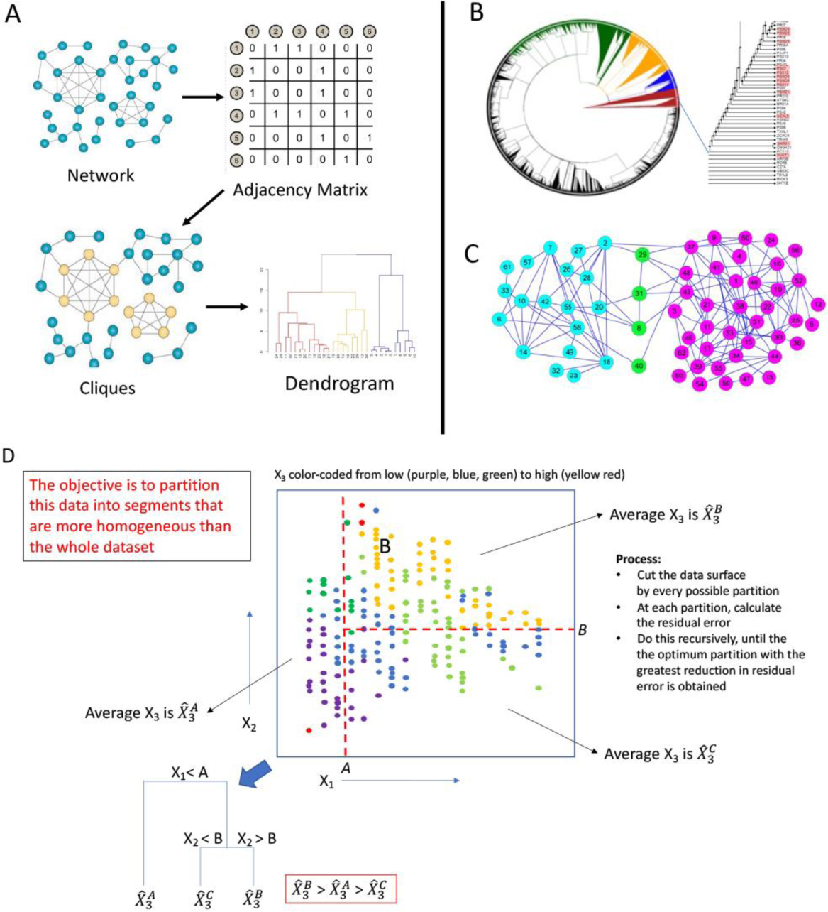
Clustering and decision trees. (A) Network clustering. Objects with certain relations are represented as graphs, from which an adjacency matrix is created, which then leads to the computation of graph properties, such as the clustering coefficient (the cliquishness of nodes) or simply a distance metric (e.g., the shortest path between node pairs, or any one of the centrality measures, etc.). Using these graph properties of similarity measures, tree-structured dendrograms are created. Inspection of the dendrograms reveals the likelihood of relatedness among nodes. (B) An example unrooted tree drawn from discrete clustering technique where each node belongs to a unique cluster of related nodes. (C) An example output of “fuzzy clustering”, where the yellow-colored nodes belong to both blue and purple node clusters. (D) A broad overview of the method of decision tree construction. Here a set of data points are represented along three dimensions (two spatial dimensions, X₁ and X₂, and one color dimension (purple, blue, green, yellow, red). The principle of decision trees is to “divide and conquer”: the data are partitioned recursively until a set of partitions that minimize the residual error due to the inhomogeneity of the data is attained. The result is a directed acyclic graph that has the power to identify important properties of the dataset.

The hierarchical clustering algorithm computes a dendrogram that assembles all elements into a single tree. For any set of N genes, an upper-diagonal similarity matrix is computed by using the metric described above, which contains similarity scores for all pairs of genes. The matrix is then examined to choose the highest value, which represents the most similar pair of genes by the similarity score. An edge is applied between these two genes (or vertices), and a gene expression profile is computed for the vertex by averaging observation for the joined elements, the two joined elements being weighted by the number of genes they contain. The similarity matrix is updated with this new vertex replacing the two joined elements, and the process is repeated (N– 1) times until only a single element remains. Here also each object (here, gene) is assigned a unique cluster membership.

Both hierarchical and K-means clustering are the most widely used clustering method in genomics related biology because the outputs of these algorithms are intuitive groupings of the genes into subclasses that can be further analyzed for additional properties. Model based approaches to systematically choose cluster size is now routine, adopting, for example, the model and the number of clusters with the largest Bayesian Information Criteria or $BIC=k\ln \left(n\right)-2\mathrm{l}\mathrm{n}\left(\widehat{L}\right)$, where k is the number of parameters estimated by the model M, $\widehat{L}=p\left(x|\theta ,M\right),$ is the maximized value of the likelihood function of the model, θ are the parameter values that maximize the likelihood function, x is the observed data and n is the number of observations (i.e., the sample size). A limitation here is that BIC cannot handle a complex collection of models, as in variable selection or feature selection in high dimensions (Schwarz 1978).

5.3. Fuzzy Clustering

Since genes or other biological objects, such as proteins or regulatory RNAs have multiple functions, it is often the case that classification of these objects into unique clusters are inadequate to capture the full extent of their biological properties. This is particularly important in datasets on molecules that interact among one another, such that a biologist wishes to infer an unknown function of a biological molecule by inferring from the functions of other members of its clustered group—inference through “guilt-by-association”. As an example, 207 out 1628 proteins in a model organism (the baker’s yeast, Saccharomyces cerevisiae) that were hand curated into specific molecular complexes, based on actual experimental observations, belonged to multiple molecular complexes. This is likely to be an underestimation. Experimental elucidation of protein function through determining molecular complexes is an expensive and time-consuming process. Therefore biologists have devised methods for determining pair-wise interaction partners of proteins. From graph models of such pairwise interaction, it should be possible to infer the best partitioning of groups of proteins through the clustering algorithm. However, clustering algorithms that classify each protein into unique clusters would miss many interesting properties. Therefore, so-called fuzzy clustering algorithms have been developed, which allows clustering of objects into multiple clusters simultaneously (Wu et al. 2014) (Fig. 4B-C). An interesting graph-based clustering algorithm, Clustering with Overlapping Neighborhood Expansion or ClusterONE (Nepusz et al. 2012), avoids this problem of non-overlapping clusters without having to impose arbitrary thresholds, and can also handle weighted edges.

ClusterONE starts with a single node (a gene or a protein), and uses a “cohesiveness” measure to estimate how likely is a group of nodes to form a cluster, V. For each vertex, $f\left(V\right)=\frac{w^{in}\left(V\right)}{w^{in}\left(V\right)+w^{bound}\left(V\right)+p\left|V\right|}$, where wⁱⁿ(V) is the total weight of edges contained entirely by a group of proteins V, w^bound(V) is the total weight of edge that connects the group with the rest of the network. The penalty factor p|V| models the uncertainty in the data and assumes undiscovered interactions in the network. The cohesiveness of protein i that is added to a node is then calculated as: $f\left(V_t\cup \left\{i\right\}\right)=\frac{w^{in}\left(V_t\right)+w_i^{in}}{w^{in}\left(V_t\right)+w^{out}\left(V_t\right)+w_i^{out}+p(\left|V_t\right|+1)}$.

The runtime of the ClusterONE algorithm depends on the exact structure of the network it is trying to cluster. While there might be artificially constructed graphs that could make ClusterONE run slowly, these graphs will most likely not be a representative of ‘real’ world datasets that the algorithm will be confronted with.

5.4. Network or graph-based clustering

Increasingly in modern biology there is a need to classify important communities of objects and their relations within large datasets of molecular interaction, such as the protein-protein interaction dataset described above, which are best represented by graphs or networks (Raval, Alpan and Ray, Animesh 2013; Charitou et al. 2016). For most standard clustering algorithms, such as K-means or hierarchical clustering, an underlying assumption is that the data (such as connectivity or distance relations) are from univariate Gaussian distributions, which is often not the case in most biological interaction networks (which generally follow a power-law distribution of their edge frequencies). Other more realistic methods of clustering are therefore needed. High-dimensional data can be simplified through graph representation that reduces the dimensionality using one of several algorithms first described as the “isometric feature mapping” or “Isomap” (Tenenbaum et al. 2000). In Isomap, a manifold, M, is chosen and the first step determines which datapoints are the nearest neighbors of M as measured by distances, d_i,j between pairs of points (i, j) in the input space X. These distances are represented as a weighted graph G over the data points, with edge weights d_X(i, j) between each pair of neighboring points. In the second step, the algorithm estimates the geodesic distances d_M(i, j) between all pairs of points on the manifold M by computing their shortest path distances d_G(i, j) in the graph G(V,E), were V and E are the nodes (vertices) and weighted edges (respectively). In the final step, classical dimensionality reduction is applied to the matrix of graph distances D_G = {d_G(i, j)}, thus constructing an embedding of the data in a d-dimensional Euclidean space Y that best preserves the manifold’s estimated intrinsic geometry. This last step minimizes a cost function that is the l₂ norm of the difference between the inner product of the matrix of graph distances D_G and that of the matrix of the embedded distances in Y (D_Y = {d_Y(i, j)}). The global minimum of this cost function is then obtained (Tenenbaum et al. 2000).

Graph based data clustering is frequently applied to genomic level association data (Liu and Barahona 2020). In a recent example, immediately upon the recognition of SARS-CoV-2 as the causative agent behind COVID-19 pandemic, the collection of human proteins that physically interact with 29 proteins encoded by the virus were rapidly determined and the ensuing interaction data were represented as clustered networks of multipartite interactions among virus-encoded and host proteins, and drug-like chemical agents that are already known to interact with the human proteins in an effort to discover drugs to ward off acute virus effects (Gordon et al. 2020). This work, though so far unsuccessful in identifying an effective drug against COVID-19, enabled rapid progress in identifying the molecular processes unleashed by the virus in the host, and subsequently an equally rapid progress in managing the clinical manifestations of severe COVID-19 infections (e.g., (Laing et al. 2020)). This instance exemplifies the need for efficient algorithms that can cluster objects on complex interaction networks.

A suite of algorithms well designed for clustering complex networks, as opposed to non-network data points, has been described (Aldecoa and Marín 2010, 2013). Within this suite, UVCluster is quite useful. However, its runtime does not scale well with size of nodes (O(n³)) (Aldecoa and Marín 2010). It is therefore important to find more efficient network clustering algorithms for the analysis of complex biological interaction datasets at the genomic scale.

A head-to-head performance comparison of a number of clustering methods ranging from K-means and hierarchical clustering to several graph-based clustering approaches indicated that the graph based methods (Zhang et al. 2005) outperform other clustering algorithms in biological (genomics) type of classification tasks (Jay et al. 2012). Nonetheless, graph based clustering algorithms including those that produce “fuzzy clusters” (i.e., data points, genes or proteins that are included in more than one cluster) have not been in wide use in current biological research mainly because of prevailing traditions in which biologists favor an unambiguous and unique assignment for a gene or protein into a cluster. In this direction several recent publications make important algorithmic contributions (Zhao and Sayed 2015; Altilio et al. 2019), and students of computational biology will do well to find their applications into biological problems. Increased future use of “fuzzy clusters” should therefore be encouraged, which might lead to novel and more realistic insights into post-genomic biology questions, for example is examining the community structures of microbial associations in the human gut for human health (Schmidt et al. 2018) or in the root-soil system of plants for a better management of global greenhouse gases (Philippot et al. 2013).

5.5. Decision Trees and Rule Mining

Decision trees are popular ML algorithms pioneered by Leo Brieman, Jerry Friedman and others are simple to understand and relatively easy to implement (Song and Lu 2015). The rational is to partition the data into every possible “cuts” and at each partition compute the residual error or the Gini coefficient or mutual entropy (Fig. 4D). This step is recursively repeated until the optimum partition that causes the maximum reduction in the residual error (or the Gini or mutual entropy) is obtained. Decision trees have the advantage of being fast as well as intuitive. However, unlike in regression analysis where the decision plane is smooth (but could be less accurate), in decision trees the decision plane is often complex and therefore introduces an increased propensity for model over-fitting. Therefore, decision trees with the simplest tree structure that causes the largest gain in residual error (or Gini or mutual entropy) reduction are favored over more complex decision trees.

Decision trees intuitively lend to the discovery of logical relationships within the data (Chen et al. 2011). Relational logic allows us to express complex data in meaningful ways. This is particularly important for genomics data, where high-dimensional data with deep structures are often presented to the investigator (Fürnkranz and Kliegr 2015). An important goal of unsupervised ML is to discover relational logical rules or rules of association that are embedded in the data. For example, an “if-then” (X ⟹ Z or, more generally, (X ∩ Y) ⟹ Z) type of association rule in static data are important for inferring important biological processes. This can be translated to a biologically meaningful statement such as, “if two genes are co-expressed in a statistically significant number of different conditions than expected by chance, then the two genes are coregulated” (Fig. 5).

Figure 5.

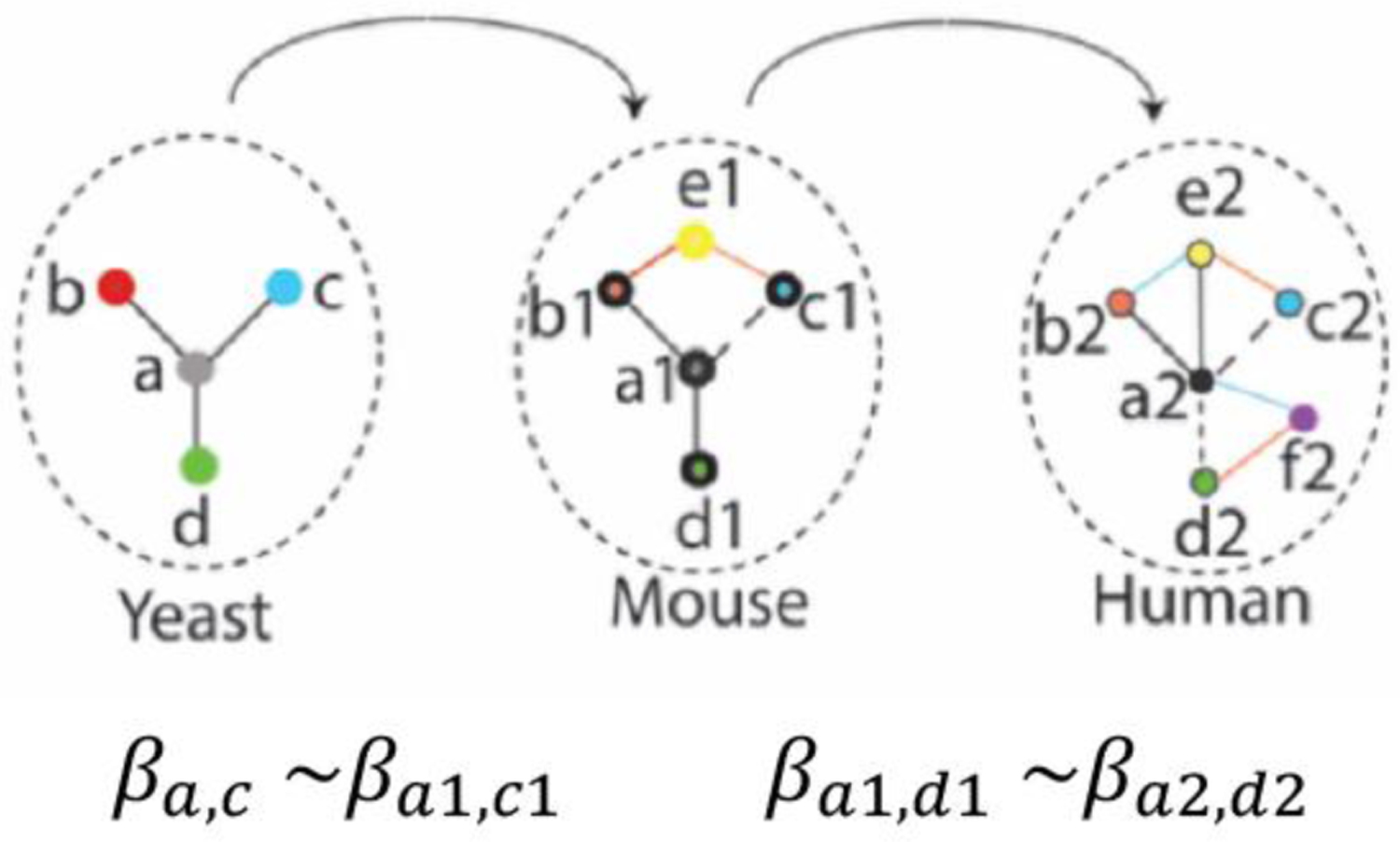
A diagrammatic example of decision rule mining by linear regression (Lam et al., 2016). Circles represent proteins within or different species of organisms, respectively. Colors define homologs of genes across species (here, yeast or mouse or human), also called orthologs. Thus, a and a1 are orthologs across species. a1 and a2 are both orthologs of a. Such orthologous relationships are deduced from sequence conservation of the proteins or their encoding genes.. When the sequence conservation is above a certain threshold, the two genes (or proteins) are accepted as “orthologs”. If proteins a and c of species 1 (yeast) are both orthologs of proteins a1 and c1 of species 2 (mouse), and if d is also an ortholog of d1’, and if it is known that a regulates both b and c, then the rule that a1 is a regulator of c1 is supported by the regression coefficients (β_a1,c1). Dashed lines indicate potential regulatory interactions.

Yet another direct relevance to personal genomics could be a Boolean association rule of the type (A∨B∨C) ∧(¬D∨ ¬E ∨ ¬ F) etc. ⟹ p (Z), in which A–F represent genes with certain variant sequences, and p (Z) is the probability of, say, a disease outcome. A logical rule such as this could be a case of 3CNF-SAT (as framed here), or an even more important one if time-series data are available, such that a “causal inference” rule of the type, [RNA of gene X] ⟹ time-delay [RNA of gene Y] can be discovered from the data (see later).

To discover the rule X ⟹ Z, one needs two pieces of information: the support, defined by $\frac{freq(X,Z)}{N}$, and the confidence, defined by $\frac{freq(X,Z)}{freq\left(X\right)}$. The challenge is because the association rules are “fuzzy” or probabilistic, and scalability of the rule extraction algorithms is an important issue due to data complexity. The process is first reduced to the construction of a search tree listing all possible ‘frequent’ fuzzy events. Such trees are then searched for fuzzy association rules by either breadth-first (first constructed by Agarwal and Srikanth, see (Toivonen 2010)) or depth-first (Zaki 2000) searches on a decision tree and then computing the individual frequencies. Genetic algorithms have been used for faster and parallel implementation of the search and pruning steps (Alcala-Fdez et al. 2011). Parallel discovery of multiple association rules have been successfully extracted from genomic DNA and protein sequences (Agapito et al., 2019; Guzzi et al., 2012), and the techniques have been applied to discover gene-expression rules related to cancer outcomes in patients (Ma and Huang 2009). Extraction of association rules from time-series data on genome-scale gene expression experiments (Segura-Delgado et al. 2020) will be described in the section on ‘explainable AI’. A yet another approach to association rule discovery in an unknown species of organism by using the information of evolutionary conserved gene/protein sequences from another organism, in which more knowledge on association rules exists, using linear regression to penalize for dissimilarities in sequences (Lam et al. 2016) (Fig. 5).

6. Supervised Machine Learning

Simply put, supervised ML requires prior examples upon which the machine is trained to make future predictions (Graphical Abstract). Supervised ML can be either a classifier, as are unsupervised MLs, or regression models, which provides a real number value associated with a predicted class. Before discussing the essential properties of a few supervised ML methods, let us motivate the discussion in the context of genome level biology with a rather fundamental biological problem.

Once a genome is sequenced, how does one find the boundaries of a gene within the monotonic strings of A, T, G and C on the genome? The formal start of a gene is that DNA base where RNA synthesis (or transcription) begins (Fig. 1). Whereas there are some commonalities in the sequence motifs near the transcription start sites, for many genes there is no obvious pattern. Beyond this point, there is a protein coding sequence that starts at a sequence of 5’ATG3’; as there are overwhelming instances of this sequence that are not the start codon, which ATG is the start codon? In eukaryotic organisms there are introns (strings within a gene that are not protein-coding), each of which is followed by another string of exon (i.e., the protein-coding Open Reading Frame or ORF) where the reading frame is re-initiated. Once the actual ORF is identified it is generally trivial to find the stop codon; however, RNA synthesis does not stop there but continues beyond the stop codon for some distance. Where does RNA synthesis terminate? There are many experimentally determined instances of each of these landmarks for many genes, but such annotation of genic landmarks is incomplete. When the genome of a previously un-sequenced organism is first sequenced, there is a need to computationally predict all its encoded genic boundaries. One of the first successful methods for gene boundary prediction (see (Brent 2005) for a review of the history of gene prediction) did not use ML, but used the Generalized Hidden Markov Model in its GENESCAN implementation (Burge and Karlin 1997). While GENSCAN was a timely and effective tool in the early days of whole genome sequencing, from which this writer had greatly benefitted at the time, it is only about 35% accurate. By contrast, a gene boundary prediction algorithm that adopted the Support Vector Machine (SVM) classifier, a supervised ML method, achieved ~50% predictive accuracy (Gross et al. 2007).

6.1. SVM

SVM is a standard tool in classification or regression (Vladimir N. Vapnik 1998) of input data, which consists of mapping the nonlinear input data to a high-dimensional space in an attempt to find a linear hyperplane in the high-dimensional space that will classify the inputs, such that a maximal separating hyperplane is constructed (Wang 2005) (Fig. 6). Two parallel hyperplanes are constructed on each side of the hyperplane that separates the data. The separating hyperplane is the hyperplane that maximizes the distance between the two parallel hyperplanes. To do this, an input feature vector x is mapped to a high-dimensional feature vector, z = ϕ (x). The high-dimensional feature space is an inner product space, called a Reproducing Kernel Hilbert Space. The aim is then to find a hyperplane, w . z + b = 0, such that the distance between the hyperplane and the closest training examples is maximal (Fig. 3). Assigning class labels y = +1 or −1 to positive and negative training samples, respectively, w b are rescaled by requiring that the closest training sample (with feature vector, say, z' and class label y' ) is such that y'(w.z' + b) = 1. With this condition, the square of the distance between the closest training example and the hyperplane is < w, w>⁻¹, where <, > is the inner product on the Reproducing Kernel Hilbert Space. By requiring that this distance is maximal, the problem can be solved as a standard dual optimization problem by quadratic programming (Cristianini and Shawe-Taylor 2000). An interesting property of SVM is that it simultaneously minimizes the empirical classification error and maximizes the geometric margin, and therefore performs well on noisy data. However, a limitation of SVM is the choice of the kernel function, because the choice of the kernel function that best classifies a given problem is an open question.

Figure 6.

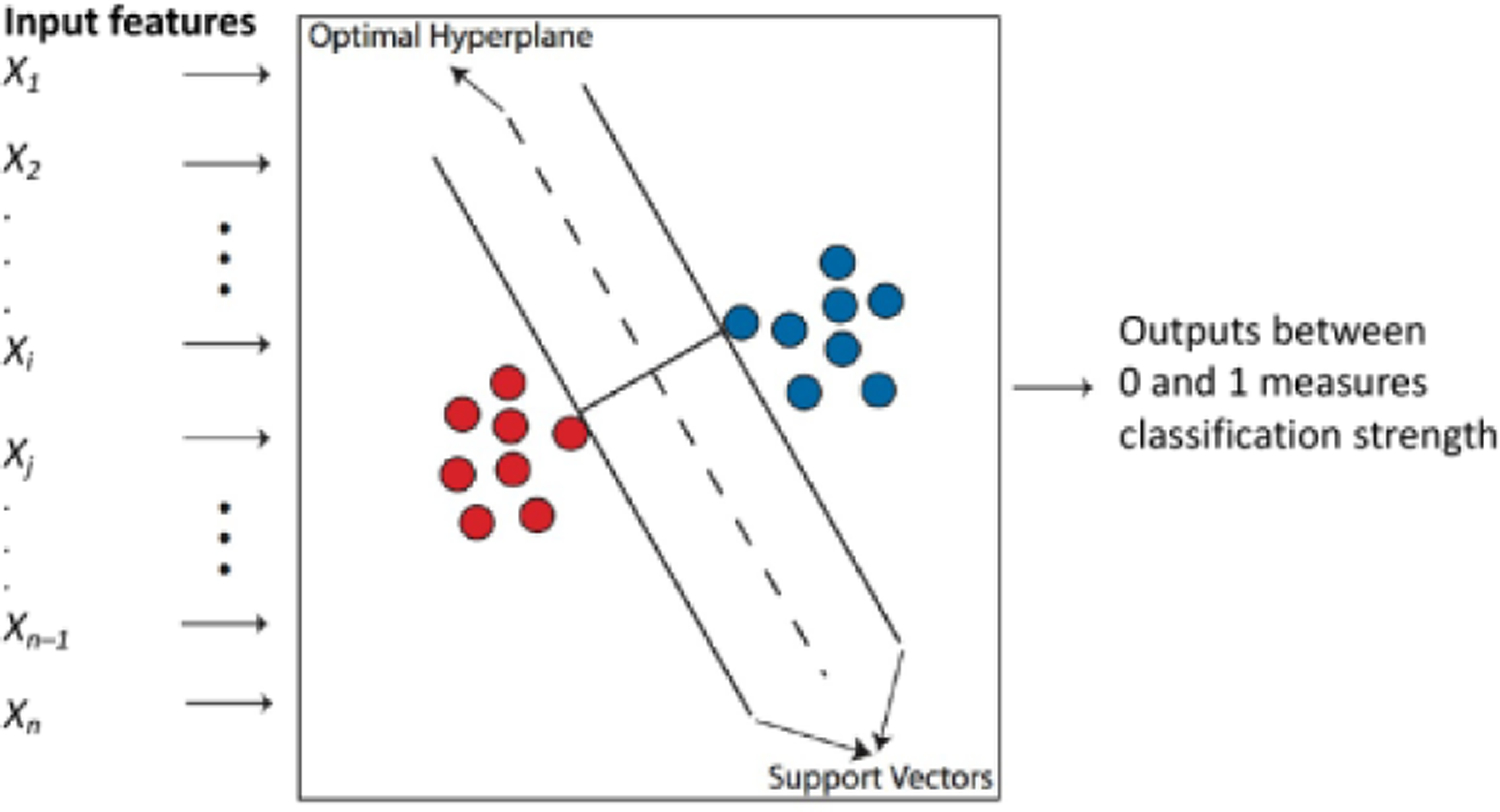
A cartoon diagram explaining the principle of Support Vector Machine (SVM). See text for explanation.

Numerous important classification problems in genomics in addition to gene prediction has been successful with SVM. Among these are miRNA target prediction (Kim et al. 2006; Yang et al. 2008), prediction and distinguishing long non-coding RNA (lncRNA) from protein-coding genes (Sun et al. 2015; Schneider et al. 2017), prediction of gene-gene interaction phenotype from protein-protein interaction network (Paladugu et al. 2008), improving and augmenting protein-protein interaction between virus encoded proteins and host proteins (Cui et al. 2012), and the prediction of protein function by kernel based integration of heterogeneous data (Brown et al. 2000; Pavlidis et al. 2002; Cui et al. 2012). In another challenging problem in biology—the prediction of protein folding—SVM has been used to classify the interface structures of pairs of interacting proteins, which helps in predicting the important amino acid residues in such interactions (Daberdaku and Ferrari 2018, 2019).

The inference of gene regulatory networks from complex genomic sequences with limited experimental data and high levels of uncertainty constitutes one of the two most challenging problems in genomics today, and SVM has been used to this end with a relatively high degree of success (Mordelet and Vert 2008; Ni et al. 2016). Metagenomics, the field of inferring communities of microbes, their properties and communal interactions through genomic DNA sequences of microbial samples taken from the population without a detailed knowledge of the constituent microbes is a challenging area of increasing significance in human health, plant-soil management in agriculture, and environmental remediation. SVM has impacted this area by enabling better de novo assembly of metagenomes from random short DNA sequences of largely unknown microbial organisms obtained from complex environmental samples (Liu et al. 2013; Zhu et al. 2014). The problem here was the assignment of pairs of partially overlapping unknown DNA sequences uniquely to a continuous genome, and thus to assign an identity to the DNA fragments in terms of their source organism within the complex sample.

6.2. Lasso and Ridge Regression

Whereas SVM has been an extremely popular ML method for the classification of complex biological information, by any means it has not been the only one. Other classification as well as regression models are increasingly being used. Generalized regression models with ℓ₁ Regularization (the Least absolute shrinkage and selection operator or Lasso Regression) has been used with relatively encouraging results in generating gene regulatory networks from multiple gene expression profile data including time-course expression profiles (Omranian et al. 2016; Nguyen and Braun 2018; Ghosh Roy et al. 2020). Lasso regression estimates the regression coefficients through an ℓ₁-norm penalized least-squares criterion. This is equivalent to minimizing the sums of squares of residuals plus an ℓ₁ penalty on the regression coefficients.

A fused ℓ₂ regression model (Ridge Regression) that learns gene a regulatory network dynamics from simulated regulatory proteins that bind to regulatory elements on the DNA, also performed well (Lam et al. 2016). In this latter method, the response variables must be solved simultaneously through vectorization if there is any chain of linked response variables connecting them, which quickly becomes computationally intractable for networks with large number of genes. However, to avoid this problem, depth-first search was used to identify linked columns of each transcription factor’s gene expression matrix which was then used to design and form response matrices through vectorization, thus segmenting the network into smaller subsets requiring fewer simultaneous equations to be solved. This method worked relatively well for prokaryotic microbes by enabling the assignment of transcription factor binding sequences to downstream regulated genes (Lam et al. 2016). A recent study explored the performance of Ridge Regression for discovering eukaryotic gene regulatory networks having significantly higher densities of linked variables, and successfully reported the assignment of nucleosome positioning patterns (the arrays of DNA-bound proteins that control local transcriptional dynamics on the eukaryotic chromosomes) to transcription factor function (Maehara and Ohkawa 2016).

6.3. Elastic Net for gene-phenotype association discovery

Genome wide association studies (GWAS) are of fundamental importance for identifying genetic variations as determinants of complex traits (traits that are determined by multiple genetic factors), such as human diseases or the food yield or the resistance to pests or pathogens by an agricultural crop, from sampling large populations (McCarthy et al. 2008). Personalized genomics critically depends on this goal. Questions in this field is of the following type: does this or that variant found for a DNA nucleotide sequence increases or decreases the susceptibility of the carrier person to a disease?

In these studies a very large number (millions) of genetic variants (typically, single nucleotide polymorphisms or SNPs) are monitored in thousands to tens of thousands of individuals. The significance of statistical association of each SNP variant with a binary property (e.g., the presence or absence of a disease) or a quantitative property (a value in the real number space, such as blood pressure or the age of onset of a disease) is computed for the test population relative to that of a control population (e.g., no disease). Unfortunately the procedure suffers from large-n/small-p problem: type I statistical error, or very high false positive rates. As a result, the significance p value is corrected for multiple hypothesis testing or false discovery rates under the assumption of independent segregation of each SNP variant in the population. This results into the opposite problem: type II error or very high false negative rates. This is because SNPs are often linked or there is selection for certain variants in the population, which leads to violation of the assumption of independent probabilities central to the correction methods, and due to the high dimensionality of the variables. As an alternative to this standard GWAS analysis, multiple regression models, specifically, Logistic (Patron et al. 2019), Lasso and Elastic Net (Waldmann et al. 2013) regressions, respectively, were used to identify SNP variants of interest. The idea is simple: Consider a multiple linear regression model, $\widehat{y}={\beta }_0+\mathbf{b}\mathit{X}+\mathit{e}$, where $\widehat{y}$ is the predicted or response variable (e.g., blood pressure or the age of disease onset), X is the n × m matrix of predictor variables (e.g., n genetic loci with m variants of each with categorical values of −1, 0, +1, for homozygosity of the major allele, heterozygosity or homozygosity for one minor allele, respectively, at the corresponding locus), β₀ is the intercept, b is a column vector that contains the regression coefficients (β₁, β₂ … β_n), and e is the vector of the corresponding error terms with a normal distribution. The Elastic Net (EN) model (Zou and Hastie 2005) of regression is based on a compromise between the ℓ₁ norm regularized Lasso penalty and the ℓ₂ norm regularized Ridge penalty functions, respectively:

$${\widehat{\beta }}_o,\widehat{\beta }=\mathrm{a}\mathrm{r}\mathrm{g}\mathrm{m}\mathrm{i}\mathrm{n}\left\{\sum _{i=1}^n{\left(y_i-{\beta }_0-\sum _{j=1}^m{\beta }_j{X}_{\mathit{ij}}\right)}^2+\lambda \sum _{j=1}^m\left[\frac{1}{2}\left(1-\alpha \right){{\beta }_j}^2+\alpha |{\beta }_j|\right]\right\}$$

Where, 0 ≤ α ≥ 1 is the penalty weight, and λ is the regularization parameter that controls shrinkage and must be tuned or chosen based on prior results.

Several studies explored regression analysis to identify and evaluate the sources of genetic variability for various phenotypes (Malo et al. 2008; Wu et al. 2009; Ayers and Cordell 2010; Waldmann et al. 2013). There is no consensus yet on whether regression models can do better than the single marker association studies (Waldmann et al. 2013). This is an important area of future research as it is intimately connected to personalized treatment of patients based on their genomic sequence data, especially for patients with certain forms of cancer, which should benefit from further exploration of ML methods.

6.4. Random Forest

Random Forest (Fig. 7A) is an ensemble decision tree-based ML method (Breiman 2001). The model grows multiple decision tree-structured classifiers {h(xΘ_k,k = 1,2 … k}, based on values of an independently distributed randomly sampled vector {Θ_k}, wherein, each tree casts a unit ‘vote’ for the most popular class based on the attributes (input or predictor variables from the matrix, x) that the tree was built on. Iteratively, decision trees with more votes are generated and these are agglomerated. The generalization error of the ensemble of decision tree classifiers depends on the strength of each tree and the correlation among them. The model predicts new data by choosing the classification that receives the most votes over all the trees. Random forest model thus reduces the variance of prediction while retaining a low bias. A lower bias and variance translate to a reduction in the prediction error and also avoids over-fitting the model to the training data. An improved version of the Random Forest implementation that iteratively removes some ‘unimportant’ features, which evidently makes the predictor more accurate, is available (Paul et al. 2018).

Figure 7.

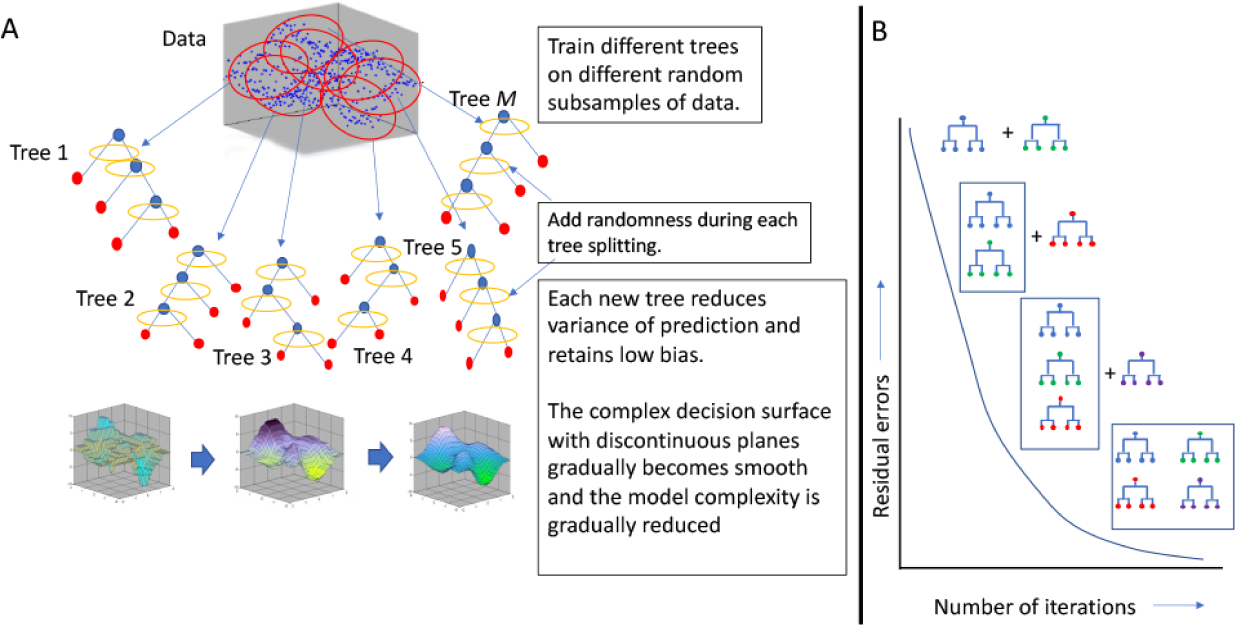
Cartoons illustrating the principles of random forest and gradient boosting machines for classification and regression. (A) Random Forest algorithms build numerous decision trees from random subsets of the data but introduces a noise at each treat splitting. The decision trees are aggregated and as a result the surface of the decision function, which is complex for each tree, is smooth when numerous trees are considered together. (B) In Gradient Boosting Machines, new trees are sequentially added to existing trees while reducing the residual error, and thus the decision function surface becomes smoother as the error decreases progressively down the error gradient. Both methods can often lead to model overfitting (due to complexity of the prediction function surface) and sometimes the models can get hung up on local minima. Therefore, rigorous testing of the prediction function using data that were not used for model training needs to be conducted.

Random Forest ML classification presents encouraging potential in molecular genomics and the prediction of disease phenotypes for genetic variants. For a genomics application, miRWalk is a Random Forest based microRNA target prediction algorithm that simultaneously produces a network-based model of interacting genes and microRNA molecules (Sticht et al. 2018). Clustered Regularly Interspaced Short Palindromic Repeats (CRISPR) have become famous over the past decade as a tool for genome engineering (Anzalone et al. 2020); a Random Forest based tool for identifying novel CRISPR arrays in bacteria has been described for biotechnology application (Wang and Liang 2017). Integration of multiple ‘omics’-scale heterogeneous datatypes for the prediction of physiological responses to treatment, such as adverse drug response or the prediction of efficacy of novel drug-like molecules, is a challenging area where Random Forest has been applied (Rahman et al. 2017). Similar applications for the prediction of novel biomarkers for clinical application, such as accurate diagnosis or prognosis of a cancer type, are possible (Toth et al. 2019). As previously discussed in the context of SVM, very large genome level datasets concerned with population genomics and metagenomics are also ripe for the application of Random Forest classification, as reported for the investigation of a possible genetic connection between intestinal microbiome composition and diabetes mellitus (Kuang et al. 2017) or fatty liver disease (Loomba et al. 2017). An emerging area of research that is likely to profoundly impact environmental resource management and reversal of global warming is the understanding of the precise role of genes in the evolution of complex ecosystems (Brieuc et al. 2018). As described above with reference to multiple regression models for capturing the effects of genetic variations in large populations through GWAS experiments, Random Forest appears to be at least as equally robust as other competing methods (Stephan et al. 2015).

6.5. Gradient Boosting Machine

As in Random Forest, Gradient Boosting Machine (GBM) also generates collections of decision tree classifiers for classification and regression. The premise of GBM is the concept of ‘boosting’ that serially adds new prediction models to the ensemble of classifiers at each iteration which gradually optimizes a cost-function over function space (Fig. 7B). A new weak, base-learner model is trained at every iteration based on the negative gradient of the loss function of the entire ensemble obtained till that point (Friedman 2001; Natekin and Knoll 2013). The weak model slowly becomes more robust as the state of the machine descends along the error gradient with the number of iterations.

GBM is finding increasing popularity in genomics style of biotechnology. A recent work used GBM to evaluate genome-wide RNA profiles for optimizing protein amount and quality of meat in pigs in response to feed programs and thus identified a series of predictor gene expression signatures (Messad et al. 2019). The reader is referred to a succinct description of this type of application in nearly any agricultural, food or drug production/manufacturing industry (González-Recio et al. 2013), with possible future application to environmental management, where the optimization of one or more products based on the genomic profiling of a population of organisms is desired. In a related application we addressed whether protein-protein interaction network has sufficient information to discriminate between interactors and non-interactor proteins with a toxic (pathogenic) version of the Huntington’s disease protein (Lokhande et al. 2016, 2018).

Like proteins, the geometry of RNA secondary structure (i.e., intramolecular folding) is an important aspect for the prediction of its biochemical function, which includes the behavior of RNA sequence variants in causing diseases and producing enzymatic reagents for synthetic biology. The classical ab initio RNA secondary structure prediction algorithms use thermodynamic free energy optimization using dynamic programming (e.g., the Nussinov algorithm (Nussinov and Jacobson 1980)); however, this imposed a severe limit to the length of the RNA that could be handled. More recently GBM has been applied with considerable success in the prediction of RNA secondary structure genome wide, which achieved high correlation (correlation coefficients >0.9) with experimentally (X-ray diffraction and Nuclear Magnetic Resonance) determined RNA secondary structures (Ke et al. 2020). This approach has now become feasible as numerous RNA secondary structure models are now available through genome-wide biochemical methods of RNA structure “model” construction (Lucks et al. 2011). These experimentally determined “model” structures, as well as a limited number of experimentally determined structures, are used as large training sets, with test sets taken from experimentally determined “gold standard” RNA structures in the GBM regression model (Ke et al. 2020).

6.6. Deep Learning

Deep Learning is the subfield of ML that is inspired by our concept of how the biological brain works through its multilayered architecture of neurons (Azulay et al. 2016), typified by the Artificial Neural Network (ANN) model of computation (see (Eraslan et al. 2019) for a recent review on Deep Learning in genomics) (Fig. 8). In general, if xⁱ be the vector of some summary statistic (input) of a dataset i, and yⁱ is the vector of response (output) variable of that dataset, and if we have n such datasets, then together {(x¹, y¹), (x² y²) … (xⁿ yⁿ)} form the training dataset used to learn the function that relates the summary statistic to the response variables. These complex nonlinear functions are expressed by the layered structures of deep neural networks. The first layer is the input layer; the subsequent layers are “hidden layers” with feed-forward as well as back-propagation topologies with adjustable weights (which recapitulate the architecture of the human brain), and the final layer is the output (or the “hypothesis” generator) layer. These so-called hidden layers introduce the computational capability of learning nonlinear functions, but also are the cause of the “black-box” nature of artificial neural networks which reduces their appeal for applications to human health (see later discussion on “explainable AI”).

Figure 8.

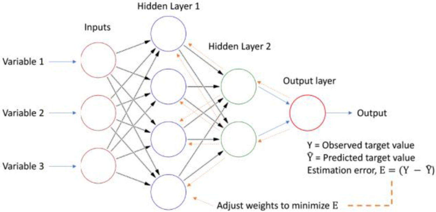
A simple four-layered artificial neural network or ANN. See text for explanation. A deep neural network contains many, many layers with fee-forward and back-propagation (arrows) in its architecture. The first layer (left) is the input layer whereas the last layer (right) is the output layer. This architecture superficially resembles the architecture of the brain. The connections (arrows) have “Hebbian” weights, which lead to complex nonlinear signal processing. The details of the signal processing function that is produced due to training are generally refractory to deconvolution, thus leading to the “black-box” nature of ANNs. Nonetheless, deep ANNs have been remarkably successful in real world data modeling, and are expected to increasingly contribute to post-genomic biology.

ANNs are algorithms that mimic the massively parallel layered architecture of a few simple but repeating computing circuits of neurons in the brain (Qian et al. 2011); a “neuron” in a neural network is a mathematical function that collects and classifies information according to a specified architecture, and is also called a perceptron. A perceptron is akin to a multiple linear regression computing unit; each perceptron feeds the output of a multiple linear regression into other perceptrons, or into an output node, though an “activation function” which may be nonlinear. Convolutional Neural Network (CNN) is the special case where the input features are an n-dimensional matrix, and mathematical convolution of multiple functions to determine the ‘shape’ of the output is used instead of matrix multiplication during multiple regression. Deep Learning involves very large (many layered) NNs or CNNs with both feed-forward and backpropagation architecture. The advantage is that Deep Learning algorithms scale significantly better than other ML algorithms with respect to size of the problem (or datasets).

One of the most noteworthy contributions of Deep Learning regression in genomics was a prediction engine for genome-wide RNA folding (Singh et al. 2019). This investigation used as training dataset (upon judiciously filtering the data for the highest confidence structures) a recently produced massive dataset of experimentally determined short RNA structures and produced an algorithm with a predictive accuracy of >90%. The researchers were able to validate all of the novel predicted structures that were subsequently tested for congruence with experimentally observed structures.

Prediction of the patterns of epigenetic modification of the genome is a computationally hard problem because of the high dimensionality and high degree of combinatorial classes that are possible. This problem is at the heart of genomics-inspired biology, and is also superbly suited for deep learning regression because of the availability of datasets that are being generated by massively parallel DNA sequencing methods coupled with identifying the boundaries of genomic DNA sequences (sequence foot-prints) occupied by epigenetically relevant proteins. The challenge is to predict the occupancy patterns of proteins at different epigenetic conditions. Recent efforts in this direction has been described in a number of publications (Wang et al. 2018; Yin et al. 2019; Beknazarov et al. 2020; Singh et al. 2016; Sekhon et al. 2018; Li et al. 2018). However, the field is still very much open because of the high degree of overfitting observed often in Deep Learning exercises with too many variables and too few training sets.

Robots that simulate human behavior are of high importance and constitute areas of massive future growth (not without its own perils if misused) for its promise of alleviating human suffering. The neural basis of higher human cognition, such as its plasticity of behavior in learning, language processing, nuance detection and display, is thought to be constructed by evolution as an organizational hierarchy in the frontal cortical lobe of the human brain. Memory is formed “bottom up” from primitive brain regions (present also in lower mammals) to the more recently developed unique brain structures of higher apes (Fuster 2004). Together, these associations constitute the “perception-action cycle”, in which external signals are “perceived” primarily by the lower level sensory receptor neurons, the outputs of which are then progressively associated ‘upwards’ in the neural hierarchy to form the “perception”, which then associate with previous memory held dispersed over large areas of the brain. The subsequent signals then are transmitted to lower areas to generate an “action”. Neuro-Inspired Companion robots (NICO) are designed to emulate this perception-reaction cycle, to emulate human emotions by learning and processing human facial changes during emotive actions. Deep neural networks using two parallel multilayered perceptrons have been used to train and refine a NICO (Barros and Wermter 2016). This multilayered perceptron used a CNN and a SOM (see above) to recognize an emotion. Once the facial features are learned using the CNN to represent the former as feature vectors, the CNN feature vector outputs were fed as inputs to the SOM. In the SOM, different layers of neurons respond to different emotions (feature vectors) and the best match between the input feature vector set and the stored feature sets were computed (Churamani et al. 2017). The resulting training for 200 rounds with human subjects was able to perform exceptionally well on correctly detecting several human emotions (anger, happiness, neutral, sadness and surprise), performing the best on anger, happiness and neutral but scored lower on detecting surprise and sadness. This reincarnation of SOM in deep learning presents exciting though yet unexplored potential for its further applications to shape recognition in postgenomic biology—for example, in automated image recognition and processing required for high-throughput single-cell based phenotypic assays during drug candidate development (Kellogg et al. 2014). A yet another unexplored area that is set for future development, which is more relevant to genomics, is to analyze human emotional disturbances by a NICO so as to correlate with the patient’s individualized genomic-level medical diagnosis. A refined measure of emotional disturbance, for which currently only self-evaluation and/or qualitative clinical evaluation exists, may provide an invaluable aid to psychometry in the future.

6.7. GNN

A particularly exciting development with the potential for robust applications to hypothesis development and causal connection detection in massive networks of genes and proteins that are generally the case in genomics is the so-called Graph Neural Network or GNN (Scarselli et al. 2009) (Fig. 9). GNNs extends the concept of neural network to graph domain representations of large datasets. GNN implements a function that maps a graph G(V,E), where V are nodes or vertices and E are edges that describe the relations between pairs of nodes, and its n nodes into an n -dimensional Euclidean space. The graphs are then encoded into feed-forward neural networks that compute a mapping of the informational influence of each node of the graph into a local transition function and a local output function. The computed values are then used to “unfold” the encoding network in which each layer corresponds to a time-instant and the connections among layers represent the connectivity of the graph. While both linear and nonlinear associations can be learned by GNNs, the cost of the learning phase, especially for nonlinear learning, is significantly higher than that of the test phase. A recent GNN implementation has performed well on existing human protein-protein interaction network data by achieving an accuracy of 99.5% (Yang et al. 2020), although the method is yet to validated for predictive accuracy on fully unknown (novel) data through biological testing.

Figure 9.

A cartoon illustrating the principle of Graph Neural Network or GNN. A simple graph (nodes are circles, edges are directed arrows) with a shaded area representing the informational influence on node 3, is explicitly encoded, which then is used to train a multi-layered feed-forward neural network by supervised learning. The layered network is then “unfolded” or decoded by the last layer and the outputs are computed. I_i are the input variables and O_i are outputs.

7. A challenge well-met: Deep Learning for protein structure prediction

One of the most challenging problems in biology is the ab initio prediction of a folded protein structure from its primary sequence (the linear sequence of amino acids in a protein) (Dill et al. 2008). The exhaustive search space for possible structures of even a relatively short protein is astronomical, implying that generating all structural variants and thus determining the minimum free energy configuration cannot be feasible. Nonetheless, proteins do manage to fold spontaneously—a situation known famously as the Levinthal’s paradox (Zwanzig et al. 1992). Levinthal’s paradox suggests that there must be favored pathways of protein folding, and ML might be one way to circumvent the high complexity combinatorial search space by using as features the physical and structural properties of a large number of proteins for which structures are solved. Consequently, Deep Learning has now been engaged widely to solve various sub-problems related to protein folding (reviewed by (Torrisi et al. 2020)). Most notably, gradient descent with a Deep Neural Network was able to train the algorithm to construct and optimize a force-field potential, which could be used to predict distances between pairs of atomic residues in their stable structural states within a protein (Senior et al. 2020).

A current incarnation of the gradient descent neural network, AlphaFold 2, made by DeepMind of Google, has reportedly outperformed every other competitor protein folding algorithm (Senior et al. 2020; Jumper et al. 2021) in the latest international “Critical Assessment of Structure Prediction” (CASP14) competition—the atomic coordinates of a few of its predicted structures are indistinguishable from those obtained by cryo-electron microscopy (at 0.3–0.6 nanometer resolution) of the folded proteins (Callaway 2020). Alphafold 2 achieves this feat by simultaneously considering multiple alignment of protein sequences, some of whose structures are already known, and by representing residue by residue interactions at a distance, in a two-track neural network. Further improvements have been made to protein structural prediction by simultaneously considering amino acid sequence pattern homology with known structures, residue-residue interactions, and possible three dimensional structures using neural network in a three-track neural network model (RoseTTAFold), and the codes are available in the public domain (Baek et al. 2021). The next logical extension of this approach has been successfully made by the latter group to predict protein interaction partners of other proteins (Humphreys et al. 2021). These breakthrough advances in protein folding prediction and computing protein-protein interaction partners are set to revolutionize genome-scale biology by potentially generating proteome-wide structural and interactome models upon which further simulation of their activities can be performed. These approaches are poised to provide unprecedented levels of quantitative sophistication in the hands of biologists and medical researchers, from cancer biologists who aim to develop an understanding of the cancer cell’s metastatic states to the biochemical engineers who wish to manipulate the carbon flux in plants and soil microorganisms to reduce the anthropogenic carbon burden. There are quite a few resources in the public domain for ab initio protein folding so as to try one’s hands at the protein-folding problem (Adhikari 2020) and per chance to improve upon these.

A related problem is the prediction of protein-ligand interaction, for which Deep Learning has been relatively successful (Ragoza et al. 2017; Stepniewska-Dziubinska et al. 2018; Zhang et al. 2019). A more complex version of the problem is to predict interaction surfaces of antibody-antibody binding, where ANN has been engaged though with relatively less success (Ansari and Raghava 2010; Liu et al. 2020). If the latter problem is solved with high precision, it should be possible one day to go in a few hours from solving the structure of a viral protein to the task of making a designed antibody reagent for a possible human clinical trial against any novel viral pandemic, a task that takes at least 4–6 months today (e.g., in the case of the SARS-CoV-2 antibody cocktail made by Regeneron Pharmaceuticals, Inc. (Baum et al. 2020)).

A related challenging problem in postgenomic biology is the computational docking of ligands (which could be small molecules, short peptides, RNA/DNA aptamers as well as full proteins) to proteins. While for small molecules and proteins of known 3-D structure docking by standard molecular dynamics simulation works well, at the genome level the challenge is to computationally dock thousands, perhaps millions, of ligands to tens of thousands of proteins. Many of the latter have no solved structures, such that protein structural prediction is a first step towards undertaking such a task. Computational docking with ML, which now out-performs classical molecular dynamics docking, is now mainstream (Kinnings et al. 2011; Hassan et al. 2018), and a recent review well describes this field (Torres et al. 2019). As predictable, biases introduced into the nonlinear regression models of deep learning and the use of numerous feature variables can be confusing; suggestions have been made for interpreting the results of such endeavors in meaningful ways (Sieg et al. 2019).

8. Newer approaches to Deep Learning

GAN:

A relatively novel deep neural network approach is the Generative Adversarial Network (GAN) (Goodfellow et al. 2014; Lan et al. 2020; Franci and Grammatico 2020). A GAN consists of two separate subnetworks—a generator and a discriminator. The objective of a GAN algorithm is to play a “mini-max” game between the two subnetworks, such that the generator’s goal is to fool the discriminator by synthesizing realistic but “fake” data from an arbitrary distribution of samples. On the other hand, the function of the discriminator neural net is to distinguish between the real data and the “fake” synthesized data. GANs have been used in several genomics applications: single-cell sequencing data, the analysis of Hi-C contact maps, and the generation of synthetic protein structures ( Lan et al., 2020). GANs are somewhat slow and difficult to train because often the solutions are stuck at local equilibria; therefore, to solve some of the problems GANs have been cast as a game-theoretic algorithm for attaining a stochastic Nash equilibrium (Franci & Grammatico, 2020). Genomics applications of this recasting of GAN is pregnant with promise, if not merely because this adversarial game strategy of two competing networks reflects evolutionary competition between species or even between neural circuits in higher brain in cognition.

9. Explainable Artificial Intelligence or XAI

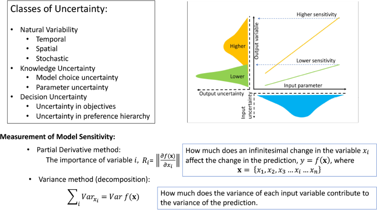
A problematic aspect of ML, especially of Deep Learning, insofar as its application to biology is concerned is the apparent black-box nature of its models due to their nested nonlinear structure. What works with high precision and recall rates might be good enough for most real-life engineering applications. In ML applications to biology, especially to human health, however, an additional layer of transparency is often demanded: an understanding of the biological significance of the important predictor variables as identified by the trained ML algorithm. While every attempt is made to identify and/or quantify the contribution of each input variable to the prediction model, often complex interaction terms preclude a clear conclusion. Philosophically, in human health applications and in genomics research, “what works” as a predictor is as important as what “the truth of nature” behind the prediction model might be. This is the goal of the so-called XAI or, interchangeably, “Explainable ML” (Samek et al. 2017). In specific applications related to the diagnosis, prognosis or treatment of human diseases, the explainability of an ML model is important for compliance purposes. In future applications to environmental problems, explainability will be an important factor because of the potential for high societal cost were the policies implemented based on a model turn to be erroneous. Comprehensibility, or “explainability” attempts to validate the reasoning behind the predictions, identifies the flaws and biases of the model, allows a deeper understanding of the problem that is claimed to be solved by the “black-box” ML model, and, finally, enables the enacting of social policies based on objective understanding or enables compliance to already-enacted social policies (Barredo Arrieta et al. 2020).

In standard statistical analysis, the contributions of the variables of importance identified by data regression are examined by different types of sensitivity analysis. The objective is to quantify the uncertainty in the output variable as an input variable is varied around a fixed point of all other variables (in the hyperspace of multiple variables) (see Fig. 10). In linear regression, the standardized regression coefficient associated with each variable quantifies the ‘influence’ of that variable to the overall model’s output. If the regression is not linear, however, as is the case with many ML methods, this method cannot be used. Other methods, such as the derivative method and variance method must be used. In the derivative method, a partial derivative of the output variable is taken with respect to each of the input variables while all other input variables are kept at a fixed point in the variable space (Fig. 10). This method is strictly local in the sense that the entire range of the input variable cannot be explored because it only examines small perturbations of each variable taken one at a time. Variance method is a global sensitivity analysis (Saltelli et al. 2007) in which the variance of the output variable is decomposed into sum of the variances of individual input variables and all of their linear combinations in a Bayesian framework (Fig. 10).

Figure 10.

Types of uncertainties and their measurements important for explainable machine learning. See text for explanation. This figure has been influenced by the discussion and illustrations in the PhD thesis of Katie Smith (Smith, 2016), University of Nottingham.

Sensitivity analysis might fail, however. For example, if sensitivity of the model to one compartment at a time is determined we neglect interactions among the compartments, which can lead to type II statistical error. Sometimes, diverse sensitivity metrics can reduce transparency of the model performance. Sensitivity analysis on too many output variables likewise can hide the key inference of the model.

Numerical support from sensitivity analysis does not by itself provide sufficient insights about the underlying mechanistic process that is discovered by the ML algorithms. Additional insights are needed to establish causality, which provides confidence as well as transferability to the knowledge thus discovered. To understand recent approaches to eXplainable ML (or, XAI) in which the notion of causality is an integral part, let us consider in a more detail a recent example of XAI for understanding the basis of ML-derived gene-regulatory pathways inferred from two kinds of data (Anguita-Ruiz et al. 2020): (1) temporal patterns of expression of genes, (2) experimentally determined binding sites of transcriptional regulatory proteins on their putative target genes. The rationale is described in Fig. 11. When such a reconstruction was applied to about 30,000 genes (both protein and RNA) in over 50 human subjects in response to an experimental condition (nutritional intervention of obese patients). The data were mined for extracting association and/or sequential rules, such as, X → Y, or if X occurs then it is likely that Y occurs too; [gene A, gene B] → time-delay [gene C, gene D, gene E] or if gene A is up-regulated and B is down regulated then with a time-delay genes C, D and E are all simultaneously up-regulated then it is likely that genes A and B are both regulators of genes C, D and E but with mutually opposite signs, and so on. From the data, such rules were extracted using input features of gene expression values, and categorial properties of known genes using an ML algorithm, CMRules (Fournier-Viger et al. 2012). The resulting rules of association were evaluated by computing the correlation between the numerical quality metrics of each association rule between gene pairs with the biological significance of the individual genes as provided by functional enrichment metrics in the Gene Ontology database (Gene Ontology Consortium 2021). If two genes are functionally related, then their biological annotations are related, which is measured by a distance metric in a directed acyclic graph derived from the ontological relations among the member genes. Thus, by combining numerical confidence scores of association rules with a measure of the relatedness of biological functions, it was possible to assess the biological validity, as opposed to merely the numerical validity, of the resulting regulatory circuits. Moreover, the notions of causality with numerical confidence values thus discovered may enable the transfer of the mechanistic knowledge to the treatment of human disease conditions, and provide a level of transparency that is needed for enacting a responsible health-care practice. To increase comprehensibility and transparency, it is important therefore not only to provide numerical comprehensibility (the exact form of the functions that relate the output to the input variables) but also to present post-hoc analysis of the results of simulations using visual representation of the relations, the range or domains of applicability, relational logical rules among the input and output variables, as well as sensitivity analysis (Barredo Arrieta et al. 2020). In short, the black-box nature of AI needs to be deconvoluted explicitly to establish expert-user confidence and, if possible, causality of the model.

Figure 11.

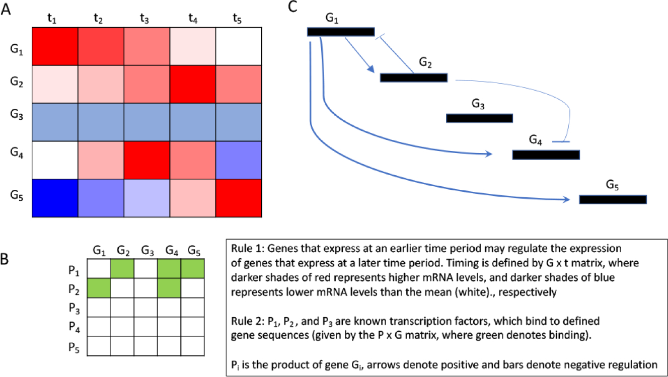
An illustration of explainable machine learning (XAI). (A) Machine learning regression determines the gene expression levels (red, increase; blue, reduction; white, steady state) at time slices t₁ through t₅. (B) Machine learning regression determines the occupancy of gene products (P_i) on the “regulatory” sequences on genes (G_i). (C) Extraction of rules from ML analysis on the outputs of (A) and (B) generates causal relations: Gene 1 regulates with a positive sign the expression of Genes 2, 4, and 5 but not of Gene 3. Gene 2 regulates the expression of Genes 1 and 4 only. Thus, the results of (A) and (B) are given a logical interpretability by (C).

10. Concluding Remarks

In a prophetic essay written in January 1991, Walter Gilbert (who shared a Nobel Prize in chemistry for the discovery of DNA sequencing method) wrote, “The new paradigm, now emerging, is that all the ‘genes’ will be known (in the sense of being resident in databases available electronically), and that the starting point of a biological investigation will be theoretical. An individual scientist will begin with a theoretical conjecture, only then turning to experiment to follow or test that hypothesis” (Gilbert 1991). This “new” paradigm in biology is now routine. AI is now making our ability to make intricately detailed, therefore quantitatively testable, theoretical conjectures possible. Its impact on medicine, public health and environmental management is already palpable though much more remains to be achieved. It is hoped that students of biology as well as computer science upon reading this review will talk to one another, and by doing so perhaps will be inspired to influence the transformation of biology in a way the author cannot imagine at the present.

References

- Adhikari B (2020) A fully open-source framework for deep learning protein real-valued distances. Sci Rep 10:13374. 10.1038/s41598-020-70181-0 [DOI] [PMC free article] [PubMed] [Google Scholar]
- Agapito G, Guzzi PH, Cannataro M (2019) Parallel extraction of association rules from genomics data. Appl Math Comput 350:434–446. 10.1016/j.amc.2017.09.026 [DOI] [Google Scholar]
- Alcala-Fdez J, Alcala R, Herrera F (2011) A Fuzzy Association Rule-Based Classification Model for High-Dimensional Problems With Genetic Rule Selection and Lateral Tuning. IEEE Trans Fuzzy Syst 19:857–872. 10.1109/TFUZZ.2011.2147794 [DOI] [Google Scholar]
- Aldecoa R, Marín I (2010) Jerarca: Efficient Analysis of Complex Networks Using Hierarchical Clustering. PLoS ONE 5:. 10.1371/journal.pone.0011585 [DOI] [PMC free article] [PubMed] [Google Scholar]
- Aldecoa R, Marín I (2013) Surprise maximization reveals the community structure of complex networks. Sci Rep 3:. 10.1038/srep01060 [DOI] [PMC free article] [PubMed] [Google Scholar]
- Altilio R, Di Lorenzo P, Panella M (2019) Distributed data clustering over networks. Pattern Recognit 93:603–620. 10.1016/j.patcog.2019.04.021 [DOI] [Google Scholar]
- Anguita-Ruiz A, Segura-Delgado A, Alcalá R, et al. (2020) eXplainable Artificial Intelligence (XAI) for the identification of biologically relevant gene expression patterns in longitudinal human studies, insights from obesity research. PLOS Comput Biol 16:e1007792. 10.1371/journal.pcbi.1007792 [DOI] [PMC free article] [PubMed] [Google Scholar]
- Ansari HR, Raghava GP (2010) Identification of conformational B-cell Epitopes in an antigen from its primary sequence. Immunome Res 6:6. 10.1186/1745-7580-6-6 [DOI] [PMC free article] [PubMed] [Google Scholar]
- Anzalone AV, Koblan LW, Liu DR (2020) Genome editing with CRISPR–Cas nucleases, base editors, transposases and prime editors. Nat Biotechnol 38:824–844. 10.1038/s41587-020-0561-9 [DOI] [PubMed] [Google Scholar]
- Ayers KL, Cordell HJ (2010) SNP selection in genome-wide and candidate gene studies via penalized logistic regression. Genet Epidemiol 34:879–891. 10.1002/gepi.20543 [DOI] [PMC free article] [PubMed] [Google Scholar]
- Azulay A, Itskovits E, Zaslaver A (2016) The C. elegans Connectome Consists of Homogenous Circuits with Defined Functional Roles. PLOS Comput Biol 12:e1005021. 10.1371/journal.pcbi.1005021 [DOI] [PMC free article] [PubMed] [Google Scholar]
- Baek M, DiMaio F, Anishchenko I, et al. (2021) Accurate prediction of protein structures and interactions using a three-track neural network. Science 373:871–876. 10.1126/science.abj8754 [DOI] [PMC free article] [PubMed] [Google Scholar]
- Barredo Arrieta A, Díaz-Rodríguez N, Del Ser J, et al. (2020) Explainable Artificial Intelligence (XAI): Concepts, taxonomies, opportunities and challenges toward responsible AI. Inf Fusion 58:82–115. 10.1016/j.inffus.2019.12.012 [DOI] [Google Scholar]
- Barros P, Wermter S (2016) Developing crossmodal expression recognition based on a deep neural model. Adapt Behav 24:373–396. 10.1177/1059712316664017 [DOI] [PMC free article] [PubMed] [Google Scholar]
- Baum A, Fulton BO, Wloga E, et al. (2020) Antibody cocktail to SARS-CoV-2 spike protein prevents rapid mutational escape seen with individual antibodies. Science 369:1014–1018. 10.1126/science.abd0831 [DOI] [PMC free article] [PubMed] [Google Scholar]
- Beknazarov N, Jin S, Poptsova M (2020) Deep learning approach for predicting functional Z-DNA regions using omics data. Sci Rep 10:19134. 10.1038/s41598-020-76203-1 [DOI] [PMC free article] [PubMed] [Google Scholar]
- Breiman L (2001) Random Forests. Mach Learn 45:5–32. 10.1023/A:1010933404324 [DOI] [Google Scholar]
- Brent MR (2005) Genome annotation past, present, and future: How to define an ORF at each locus. Genome Res 15:1777–1786. 10.1101/gr.3866105 [DOI] [PubMed] [Google Scholar]
- Brieuc MSO, Waters CD, Drinan DP, Naish KA (2018) A practical introduction to Random Forest for genetic association studies in ecology and evolution. Mol Ecol Resour 18:755–766. 10.1111/1755-0998.12773 [DOI] [PubMed] [Google Scholar]
- Brown MPS, Grundy WN, Lin D, et al. (2000) Knowledge-based analysis of microarray gene expression data by using support vector machines. Proc Natl Acad Sci 97:262–267. 10.1073/pnas.97.1.262 [DOI] [PMC free article] [PubMed] [Google Scholar]
- Burge C, Karlin S (1997) Prediction of complete gene structures in human genomic DNA11Edited by F. E. Cohen. J Mol Biol 268:78–94. 10.1006/jmbi.1997.0951 [DOI] [PubMed] [Google Scholar]
- Callaway E (2020) ‘It will change everything’: DeepMind’s AI makes gigantic leap in solving protein structures. Nature 588:203–204. 10.1038/d41586-020-03348-4 [DOI] [PubMed] [Google Scholar]
- Charitou T, Bryan K, Lynn DJ (2016) Using biological networks to integrate, visualize and analyze genomics data. Genet Sel Evol 48:27. 10.1186/s12711-016-0205-1 [DOI] [PMC free article] [PubMed] [Google Scholar]
- Chen X, Wang M, Zhang H (2011) The use of classification trees for bioinformatics. Wiley Interdiscip Rev Data Min Knowl Discov 1:55–63. 10.1002/widm.14 [DOI] [PMC free article] [PubMed] [Google Scholar]
- Churamani N, Kerzel M, Strahl E, et al. (2017) Teaching emotion expressions to a human companion robot using deep neural architectures. In: 2017 International Joint Conference on Neural Networks (IJCNN). pp 627–634 [Google Scholar]
- Cristianini N, Shawe-Taylor J (2000) An Introduction to Support Vector Machines and Other Kernel-based Learning Methods. Cambridge University Press, Cambridge [Google Scholar]
- Cui G, Fang C, Han K (2012) Prediction of protein-protein interactions between viruses and human by an SVM model. BMC Bioinformatics 13:S5. 10.1186/1471-2105-13-S7-S5 [DOI] [PMC free article] [PubMed] [Google Scholar]
- Daberdaku S, Ferrari C (2018) Exploring the potential of 3D Zernike descriptors and SVM for protein-protein interface prediction. BMC Bioinformatics 19:35. 10.1186/s12859-018-2043-3 [DOI] [PMC free article] [PubMed] [Google Scholar]
- Daberdaku S, Ferrari C (2019) Antibody interface prediction with 3D Zernike descriptors and SVM. Bioinforma Oxf Engl 35:1870–1876. 10.1093/bioinformatics/bty918 [DOI] [PubMed] [Google Scholar]
- Dey D, Slomka PJ, Leeson P, et al. (2019) Artificial Intelligence in Cardiovascular Imaging: JACC State-of-the-Art Review. J Am Coll Cardiol 73:1317–1335. 10.1016/j.jacc.2018.12.054 [DOI] [PMC free article] [PubMed] [Google Scholar]
- Dill KA, Ozkan SB, Shell MS, Weikl TR (2008) The Protein Folding Problem. Annu Rev Biophys 37:289–316. 10.1146/annurev.biophys.37.092707.153558 [DOI] [PMC free article] [PubMed] [Google Scholar]
- Dudley JT, Karczewski KJ (2013) Exploring Personal Genomics. OUP Oxford [Google Scholar]
- Eraslan G, Avsec Ž, Gagneur J, Theis FJ (2019) Deep learning: new computational modelling techniques for genomics. Nat Rev Genet 20:389–403. 10.1038/s41576-019-0122-6 [DOI] [PubMed] [Google Scholar]
- Fournier-Viger P, Faghihi U, Nkambou R, Nguifo EM (2012) CMRules: Mining sequential rules common to several sequences. Knowl-Based Syst 25:63–76. 10.1016/j.knosys.2011.07.005 [DOI] [Google Scholar]
- Franci B, Grammatico S (2020) A game-theoretic approach for Generative Adversarial Networks. ArXiv200313637 Cs Math Stat [Google Scholar]
- Friedman JH (2001) Greedy function approximation: A gradient boosting machine. Ann Stat 29:1189–1232. 10.1214/aos/1013203451 [DOI] [Google Scholar]
- Fürnkranz J, Kliegr T (2015) A Brief Overview of Rule Learning. In: Bassiliades N, Gottlob G, Sadri F, et al. (eds) Rule Technologies: Foundations, Tools, and Applications. Springer International Publishing, Cham, pp 54–69 [Google Scholar]
- Fuster JM (2004) Upper processing stages of the perception–action cycle. Trends Cogn Sci 8:143–145. 10.1016/j.tics.2004.02.004 [DOI] [PubMed] [Google Scholar]
- Gene Ontology Consortium (2021) The Gene Ontology resource: enriching a GOld mine. Nucleic Acids Res 49:D325–D334. 10.1093/nar/gkaa1113 [DOI] [PMC free article] [PubMed] [Google Scholar]
- Ghosh Roy G, Geard N, Verspoor K, He S (2020) PoLoBag: Polynomial Lasso Bagging for signed gene regulatory network inference from expression data. Bioinformatics. 10.1093/bioinformatics/btaa651 [DOI] [PubMed] [Google Scholar]
- Gilbert W (1991) Towards a paradigm shift in biology. Nature 349:99–99. 10.1038/349099a0 [DOI] [PubMed] [Google Scholar]
- González-Recio O, Jiménez-Montero JA, Alenda R (2013) The gradient boosting algorithm and random boosting for genome-assisted evaluation in large data sets. J Dairy Sci 96:614–624. 10.3168/jds.2012-5630 [DOI] [PubMed] [Google Scholar]
- Goodfellow IJ, Pouget-Abadie J, Mirza M, et al. (2014) Generative Adversarial Networks. ArXiv14062661 Cs Stat [Google Scholar]
- Gordon DE, Jang GM, Bouhaddou M, et al. (2020) A SARS-CoV-2 protein interaction map reveals targets for drug repurposing. Nature 583:459–468. 10.1038/s41586-020-2286-9 [DOI] [PMC free article] [PubMed] [Google Scholar]
- Gross SS, Do CB, Sirota M, Batzoglou S (2007) CONTRAST: a discriminative, phylogeny-free approach to multiple informant de novogene prediction. Genome Biol 8:R269. 10.1186/gb-2007-8-12-r269 [DOI] [PMC free article] [PubMed] [Google Scholar]
- Guyon I, Elisseeff A (2003) An Introduction to Variable and Feature Selection. J Mach Learn Res 3:1157–1182 [Google Scholar]
- Guzzi PH, Mina M, Guerra C, Cannataro M (2012) Semantic similarity analysis of protein data: assessment with biological features and issues. Brief Bioinform 13:569–585. 10.1093/bib/bbr066 [DOI] [PubMed] [Google Scholar]
- Hassan M, Mogollon DC, Fuentes O, Sirimulla S (2018) DLSCORE: A Deep Learning Model for Predicting Protein-Ligand Binding Affinities. 10.26434/chemrxiv.6159143.v1 [DOI] [Google Scholar]
- Hessler G, Baringhaus K-H (2018) Artificial Intelligence in Drug Design. Molecules 23:2520. 10.3390/molecules23102520 [DOI] [PMC free article] [PubMed] [Google Scholar]
- Huang S, Cai N, Pacheco PP, et al. (2018) Applications of Support Vector Machine (SVM) Learning in Cancer Genomics. Cancer Genomics Proteomics 15:41–51. 10.21873/cgp.20063 [DOI] [PMC free article] [PubMed] [Google Scholar]
- Humphreys IR, Pei J, Baek M, et al. (2021) Computed structures of core eukaryotic protein complexes. Science 0:eabm4805. 10.1126/science.abm4805 [DOI] [PMC free article] [PubMed] [Google Scholar]
- Jay JJ, Eblen JD, Zhang Y, et al. (2012) A systematic comparison of genome-scale clustering algorithms. BMC Bioinformatics 13:S7. 10.1186/1471-2105-13-S10-S7 [DOI] [PMC free article] [PubMed] [Google Scholar]
- Jumper J, Evans R, Pritzel A, et al. (2021) Highly accurate protein structure prediction with AlphaFold. Nature 596:583–589. 10.1038/s41586-021-03819-2 [DOI] [PMC free article] [PubMed] [Google Scholar]
- Ke Y, Rao J, Zhao H, et al. (2020) Accurate prediction of genome-wide RNA secondary structure profile based on extreme gradient boosting. Bioinformatics 36:4576–4582. 10.1093/bioinformatics/btaa534 [DOI] [PubMed] [Google Scholar]
- Keinan A, Clark AG (2012) Recent Explosive Human Population Growth Has Resulted in an Excess of Rare Genetic Variants. Science 336:740–743. 10.1126/science.1217283 [DOI] [PMC free article] [PubMed] [Google Scholar]
- Kellogg RA, Gómez-Sjöberg R, Leyrat AA, Tay S (2014) High-throughput microfluidic single-cell analysis pipeline for studies of signaling dynamics. Nat Protoc 9:1713–1726. 10.1038/nprot.2014.120 [DOI] [PubMed] [Google Scholar]
- Kim S-K, Nam J-W, Rhee J-K, et al. (2006) miTarget: microRNA target gene prediction using a support vector machine. BMC Bioinformatics 7:411. 10.1186/1471-2105-7-411 [DOI] [PMC free article] [PubMed] [Google Scholar]
- Kinnings SL, Liu N, Tonge PJ, et al. (2011) A machine learning based method to improve docking scoring functions and its application to drug repurposing. J Chem Inf Model 51:408–419. 10.1021/ci100369f [DOI] [PMC free article] [PubMed] [Google Scholar]
- Kohonen T (1990) The self-organizing map. Proc IEEE 78:1464–1480. 10.1109/5.58325 [DOI] [Google Scholar]
- Kong Y, Qu D, Chen X, et al. (2016) Self-Organizing Map (SOM) and Support Vector Machine (SVM) Models for the Prediction of Human Epidermal Growth Factor Receptor (EGFR/ ErbB-1) Inhibitors. Comb Chem High Throughput Screen 19:400–411. 10.2174/1386207319666160414105044 [DOI] [PubMed] [Google Scholar]
- Kuang Y-S, Lu J-H, Li S-H, et al. (2017) Connections between the human gut microbiome and gestational diabetes mellitus. GigaScience 6:1–12. 10.1093/gigascience/gix058 [DOI] [PMC free article] [PubMed] [Google Scholar]
- Laing AG, Lorenc A, del Molino del Barrio I, et al. (2020) A dynamic COVID-19 immune signature includes associations with poor prognosis. Nat Med 26:1623–1635. 10.1038/s41591-020-1038-6 [DOI] [PubMed] [Google Scholar]
- Lam KY, Westrick ZM, Müller CL, et al. (2016) Fused Regression for Multi-source Gene Regulatory Network Inference. PLOS Comput Biol 12:e1005157. 10.1371/journal.pcbi.1005157 [DOI] [PMC free article] [PubMed] [Google Scholar]
- Lan L, You L, Zhang Z, et al. (2020) Generative Adversarial Networks and Its Applications in Biomedical Informatics. Front Public Health 8:. 10.3389/fpubh.2020.00164 [DOI] [PMC free article] [PubMed] [Google Scholar]
- Li Y, Shi W, Wasserman WW (2018) Genome-wide prediction of cis-regulatory regions using supervised deep learning methods. BMC Bioinformatics 19:202. 10.1186/s12859-018-2187-1 [DOI] [PMC free article] [PubMed] [Google Scholar]
- Liu T, Shi K, Li W (2020) Deep learning methods improve linear B-cell epitope prediction. BioData Min 13:1. 10.1186/s13040-020-00211-0 [DOI] [PMC free article] [PubMed] [Google Scholar]
- Liu Y, Guo J, Hu G, Zhu H (2013) Gene prediction in metagenomic fragments based on the SVM algorithm. BMC Bioinformatics 14:S12. 10.1186/1471-2105-14-S5-S12 [DOI] [PMC free article] [PubMed] [Google Scholar]
- Liu Z, Barahona M (2020) Graph-based data clustering via multiscale community detection. Appl Netw Sci 5:1–20. 10.1007/s41109-019-0248-7 [DOI] [Google Scholar]
- Lokhande S, Koo S, Ray A (2018) Supervised Machine Learning with Protein Structural and Network Topological Features Predicts Physical Interactors of the Human Huntingtons Disease Protein. In: 2018 International Conference on Computational Science and Computational Intelligence (CSCI). pp 1362–1367 [Google Scholar]
- Lokhande S, Patra BN, Ray A (2016) A link between chromatin condensation mechanisms and Huntington’s disease: connecting the dots. Mol Biosyst 12:3515–3529. 10.1039/C6MB00598E [DOI] [PubMed] [Google Scholar]
- Loomba R, Seguritan V, Li W, et al. (2017) Gut Microbiome-Based Metagenomic Signature for Non-invasive Detection of Advanced Fibrosis in Human Nonalcoholic Fatty Liver Disease. Cell Metab 25:1054–1062.e5. 10.1016/j.cmet.2017.04.001 [DOI] [PMC free article] [PubMed] [Google Scholar]
- Lucks JB, Mortimer SA, Trapnell C, et al. (2011) Multiplexed RNA structure characterization with selective 2′-hydroxyl acylation analyzed by primer extension sequencing (SHAPE-Seq). Proc Natl Acad Sci 108:11063–11068. 10.1073/pnas.1106501108 [DOI] [PMC free article] [PubMed] [Google Scholar]
- Ma S, Huang J (2009) Regularized gene selection in cancer microarray meta-analysis. BMC Bioinformatics 10:1. 10.1186/1471-2105-10-1 [DOI] [PMC free article] [PubMed] [Google Scholar]
- Maehara K, Ohkawa Y (2016) Exploration of nucleosome positioning patterns in transcription factor function. Sci Rep 6:19620. 10.1038/srep19620 [DOI] [PMC free article] [PubMed] [Google Scholar]
- Malo N, Libiger O, Schork NJ (2008) Accommodating linkage disequilibrium in genetic-association analyses via ridge regression. Am J Hum Genet 82:375–385. 10.1016/j.ajhg.2007.10.012 [DOI] [PMC free article] [PubMed] [Google Scholar]
- Matullo G, Gaetano CD, Guarrera S (2013) Next generation sequencing and rare genetic variants: From human population studies to medical genetics. Environ Mol Mutagen 54:518–532. 10.1002/em.21799 [DOI] [PubMed] [Google Scholar]
- McCarthy MI, Abecasis GR, Cardon LR, et al. (2008) Genome-wide association studies for complex traits: consensus, uncertainty and challenges. Nat Rev Genet 9:356–369. 10.1038/nrg2344 [DOI] [PubMed] [Google Scholar]
- Messad F, Louveau I, Koffi B, et al. (2019) Investigation of muscle transcriptomes using gradient boosting machine learning identifies molecular predictors of feed efficiency in growing pigs. BMC Genomics 20:659. 10.1186/s12864-019-6010-9 [DOI] [PMC free article] [PubMed] [Google Scholar]
- Mordelet F, Vert J-P (2008) SIRENE: supervised inference of regulatory networks. Bioinformatics 24:i76–i82. 10.1093/bioinformatics/btn273 [DOI] [PubMed] [Google Scholar]
- Natekin A, Knoll A (2013) Gradient boosting machines, a tutorial. Front Neurorobotics 7:. 10.3389/fnbot.2013.00021 [DOI] [PMC free article] [PubMed] [Google Scholar]
- Nepusz T, Yu H, Paccanaro A (2012) Detecting overlapping protein complexes in protein-protein interaction networks. Nat Methods 9:471–472. 10.1038/nmeth.1938 [DOI] [PMC free article] [PubMed] [Google Scholar]
- Nguyen P, Braun R (2018) Time-lagged Ordered Lasso for network inference. BMC Bioinformatics 19:545. 10.1186/s12859-018-2558-7 [DOI] [PMC free article] [PubMed] [Google Scholar]
- Ni Y, Aghamirzaie D, Elmarakeby H, et al. (2016) A Machine Learning Approach to Predict Gene Regulatory Networks in Seed Development in Arabidopsis. Front Plant Sci 7:. 10.3389/fpls.2016.01936 [DOI] [PMC free article] [PubMed] [Google Scholar]
- Nussinov R, Jacobson AB (1980) Fast algorithm for predicting the secondary structure of single-stranded RNA. Proc Natl Acad Sci U S A 77:6309–6313 [DOI] [PMC free article] [PubMed] [Google Scholar]
- Omranian N, Eloundou-Mbebi JMO, Mueller-Roeber B, Nikoloski Z (2016) Gene regulatory network inference using fused LASSO on multiple data sets. Sci Rep 6:20533. 10.1038/srep20533 [DOI] [PMC free article] [PubMed] [Google Scholar]
- Paladugu SR, Zhao S, Ray A, Raval A (2008) Mining protein networks for synthetic genetic interactions. BMC Bioinformatics 9:426. 10.1186/1471-2105-9-426 [DOI] [PMC free article] [PubMed] [Google Scholar]
- Patron J, Serra-Cayuela A, Han B, et al. (2019) Assessing the performance of genome-wide association studies for predicting disease risk. PLOS ONE 14:e0220215. 10.1371/journal.pone.0220215 [DOI] [PMC free article] [PubMed] [Google Scholar]
- Paul A, Mukherjee DP, Das P, et al. (2018) Improved Random Forest for Classification. IEEE Trans Image Process Publ IEEE Signal Process Soc 27:4012–4024. 10.1109/TIP.2018.2834830 [DOI] [PubMed] [Google Scholar]
- Pavlidis P, Weston J, Cai J, Noble WS (2002) Learning Gene Functional Classifications from Multiple Data Types. J Comput Biol 9:401–411. 10.1089/10665270252935539 [DOI] [PubMed] [Google Scholar]
- Philippot L, Raaijmakers JM, Lemanceau P, van der Putten WH (2013) Going back to the roots: the microbial ecology of the rhizosphere. Nat Rev Microbiol 11:789–799. 10.1038/nrmicro3109 [DOI] [PubMed] [Google Scholar]
- Qian J, Hintze A, Adami C (2011) Colored Motifs Reveal Computational Building Blocks in the C. elegans Brain. PLOS ONE 6:e17013. 10.1371/journal.pone.0017013 [DOI] [PMC free article] [PubMed] [Google Scholar]
- Ragoza M, Hochuli J, Idrobo E, et al. (2017) Protein–Ligand Scoring with Convolutional Neural Networks. J Chem Inf Model 57:942–957. 10.1021/acs.jcim.6b00740 [DOI] [PMC free article] [PubMed] [Google Scholar]
- Rahman R, Otridge J, Pal R (2017) IntegratedMRF: random forest-based framework for integrating prediction from different data types. Bioinforma Oxf Engl 33:1407–1410. 10.1093/bioinformatics/btw765 [DOI] [PMC free article] [PubMed] [Google Scholar]
- Raval Alpan, Ray Animesh (2013) Introduction to Biological Networks. Chapman and Hall/CRC, Boca Raton, London, New York [Google Scholar]
- Rehm HL (2017) Evolving health care through personal genomics. Nat Rev Genet 18:259–267. 10.1038/nrg.2016.162 [DOI] [PMC free article] [PubMed] [Google Scholar]
- Roussinov DG, Chen H (1998) A Scalable Self-organizing Map Algorithm for Textual Classification: A Neural Network Approach to Thesaurus Generation. Commun Cogn Artif Intell Spring 15:81–112 [Google Scholar]
- Saltelli A, Ratto M, Andres T, et al. (2007) Global Sensitivity Analysis: The Primer. Publisher: John Wiley & Sons, Australia [Google Scholar]
- Samek W, Wiegand T, Müller K-R (2017) Explainable Artificial Intelligence: Understanding, Visualizing and Interpreting Deep Learning Models. ArXiv170808296 Cs Stat [Google Scholar]
- Scarselli F, Gori M, Tsoi AC, et al. (2009) The Graph Neural Network Model. IEEE Trans Neural Netw 20:61–80. 10.1109/TNN.2008.2005605 [DOI] [PubMed] [Google Scholar]
- Schmidt TSB, Raes J, Bork P (2018) The Human Gut Microbiome: From Association to Modulation. Cell 172:1198–1215. 10.1016/j.cell.2018.02.044 [DOI] [PubMed] [Google Scholar]
- Schneider HW, Raiol T, Brigido MM, et al. (2017) A Support Vector Machine based method to distinguish long non-coding RNAs from protein coding transcripts. BMC Genomics 18:804. 10.1186/s12864-017-4178-4 [DOI] [PMC free article] [PubMed] [Google Scholar]
- Schwarz G (1978) Estimating the Dimension of a Model. Ann Stat 6:461–464 [Google Scholar]
- Segura-Delgado A, Gacto MJ, Alcalá R, Alcalá-Fdez J (2020) Temporal association rule mining: An overview considering the time variable as an integral or implied component. WIREs Data Min Knowl Discov 10:e1367. 10.1002/widm.1367 [DOI] [Google Scholar]
- Sekhon A, Singh R, Qi Y (2018) DeepDiff: DEEP-learning for predicting DIFFerential gene expression from histone modifications. Bioinformatics 34:i891–i900. 10.1093/bioinformatics/bty612 [DOI] [PubMed] [Google Scholar]
- Senior AW, Evans R, Jumper J, et al. (2020) Improved protein structure prediction using potentials from deep learning. Nature 577:706–710. 10.1038/s41586-019-1923-7 [DOI] [PubMed] [Google Scholar]
- Sieg J, Flachsenberg F, Rarey M (2019) In Need of Bias Control: Evaluating Chemical Data for Machine Learning in Structure-Based Virtual Screening. J Chem Inf Model 59:947–961. 10.1021/acs.jcim.8b00712 [DOI] [PubMed] [Google Scholar]
- Singh J, Hanson J, Paliwal K, Zhou Y (2019) RNA secondary structure prediction using an ensemble of two-dimensional deep neural networks and transfer learning. Nat Commun 10:5407. 10.1038/s41467-019-13395-9 [DOI] [PMC free article] [PubMed] [Google Scholar]
- Singh R, Lanchantin J, Robins G, Qi Y (2016) DeepChrome: deep-learning for predicting gene expression from histone modifications. Bioinforma Oxf Engl 32:i639–i648. 10.1093/bioinformatics/btw427 [DOI] [PubMed] [Google Scholar]
- Smith KA (2016) Investigating uncertainty in global hydrology modelling. http://eprints.nottingham.ac.uk/31875/. Accessed 8 Aug 2021
- Song Y, Lu Y (2015) Decision tree methods: applications for classification and prediction. Shanghai Arch Psychiatry 27:130–135. 10.11919/j.issn.1002-0829.215044 [DOI] [PMC free article] [PubMed] [Google Scholar]
- Stephan J, Stegle O, Beyer A (2015) A random forest approach to capture genetic effects in the presence of population structure. Nat Commun 6:7432. 10.1038/ncomms8432 [DOI] [PubMed] [Google Scholar]
- Stepniewska-Dziubinska MM, Zielenkiewicz P, Siedlecki P (2018) Development and evaluation of a deep learning model for protein–ligand binding affinity prediction. Bioinformatics 34:3666–3674. 10.1093/bioinformatics/bty374 [DOI] [PMC free article] [PubMed] [Google Scholar]
- Sticht C, De La Torre C, Parveen A, Gretz N (2018) miRWalk: An online resource for prediction of microRNA binding sites. PloS One 13:e0206239. 10.1371/journal.pone.0206239 [DOI] [PMC free article] [PubMed] [Google Scholar]
- Sun L, Liu H, Zhang L, Meng J (2015) lncRScan-SVM: A Tool for Predicting Long Non-Coding RNAs Using Support Vector Machine. PLOS ONE 10:e0139654. 10.1371/journal.pone.0139654 [DOI] [PMC free article] [PubMed] [Google Scholar]
- Tamayo P, Slonim D, Mesirov J, et al. (1999) Interpreting patterns of gene expression with self-organizing maps: Methods and application to hematopoietic differentiation. Proc Natl Acad Sci 96:2907–2912. 10.1073/pnas.96.6.2907 [DOI] [PMC free article] [PubMed] [Google Scholar]
- Tenenbaum JB, de Silva V, Langford JC (2000) A Global Geometric Framework for Nonlinear Dimensionality Reduction. Science 290:2319–2323. 10.1126/science.290.5500.2319 [DOI] [PubMed] [Google Scholar]
- Toivonen H (2010) Apriori Algorithm. In: Sammut C, Webb GI (eds) Encyclopedia of Machine Learning. Springer US, Boston, MA, pp 39–40 [Google Scholar]
- Torres PHM, Sodero ACR, Jofily P, Silva-Jr FP (2019) Key Topics in Molecular Docking for Drug Design. Int J Mol Sci 20:4574. 10.3390/ijms20184574 [DOI] [PMC free article] [PubMed] [Google Scholar]
- Torrisi M, Pollastri G, Le Q (2020) Deep learning methods in protein structure prediction. Comput Struct Biotechnol J 18:1301–1310. 10.1016/j.csbj.2019.12.011 [DOI] [PMC free article] [PubMed] [Google Scholar]
- Toth R, Schiffmann H, Hube-Magg C, et al. (2019) Random forest-based modelling to detect biomarkers for prostate cancer progression. Clin Epigenetics 11:148. 10.1186/s13148-019-0736-8 [DOI] [PMC free article] [PubMed] [Google Scholar]
- Vapnik Vladimir N. (1998) Statistical Learning Theory. Wiley, New York, NY, USA [Google Scholar]
- Waldmann P, Mészáros G, Gredler B, et al. (2013) Evaluation of the lasso and the elastic net in genome-wide association studies. Front Genet 4:. 10.3389/fgene.2013.00270 [DOI] [PMC free article] [PubMed] [Google Scholar]
- Wang K, Liang C (2017) CRF: detection of CRISPR arrays using random forest. PeerJ 5:e3219. 10.7717/peerj.3219 [DOI] [PMC free article] [PubMed] [Google Scholar]
- Wang L (2005) Support Vector Machines: Theory and Applications. Springer Science & Business Media [Google Scholar]
- Wang M, Tai C, E W, Wei L (2018) DeFine: deep convolutional neural networks accurately quantify intensities of transcription factor-DNA binding and facilitate evaluation of functional non-coding variants. Nucleic Acids Res 46:e69–e69. 10.1093/nar/gky215 [DOI] [PMC free article] [PubMed] [Google Scholar]
- Williams AM, Liu Y, Regner KR, et al. (2018) Artificial intelligence, physiological genomics, and precision medicine. Physiol Genomics 50:237–243. 10.1152/physiolgenomics.00119.2017 [DOI] [PMC free article] [PubMed] [Google Scholar]
- Wu H, Gao L, Dong J, Yang X (2014) Detecting Overlapping Protein Complexes by Rough-Fuzzy Clustering in Protein-Protein Interaction Networks. PLoS ONE 9:e91856. 10.1371/journal.pone.0091856 [DOI] [PMC free article] [PubMed] [Google Scholar]
- Wu TT, Chen YF, Hastie T, et al. (2009) Genome-wide association analysis by lasso penalized logistic regression. Bioinforma Oxf Engl 25:714–721. 10.1093/bioinformatics/btp041 [DOI] [PMC free article] [PubMed] [Google Scholar]
- Yang F, Fan K, Song D, Lin H (2020) Graph-based prediction of Protein-protein interactions with attributed signed graph embedding. BMC Bioinformatics 21:323. 10.1186/s12859-020-03646-8 [DOI] [PMC free article] [PubMed] [Google Scholar]
- Yang Y, Wang Y-P, Li K-B (2008) MiRTif: a support vector machine-based microRNA target interaction filter. BMC Bioinformatics 9:S4. 10.1186/1471-2105-9-S12-S4 [DOI] [PMC free article] [PubMed] [Google Scholar]
- Yin Q, Wu M, Liu Q, et al. (2019) DeepHistone: a deep learning approach to predicting histone modifications. BMC Genomics 20:193. 10.1186/s12864-019-5489-4 [DOI] [PMC free article] [PubMed] [Google Scholar]
- Zaki MJ (2000) Scalable algorithms for association mining. IEEE Trans Knowl Data Eng 12:372–390. 10.1109/69.846291 [DOI] [Google Scholar]
- Zhang H, Liao L, Saravanan KM, et al. (2019) DeepBindRG: a deep learning based method for estimating effective protein–ligand affinity. PeerJ 7:e7362. 10.7717/peerj.7362 [DOI] [PMC free article] [PubMed] [Google Scholar]
- Zhang Y, Abu-Khzam FN, Baldwin NE, et al. (2005) Genome-Scale Computational Approaches to Memory-Intensive Applications in Systems Biology. In: Proceedings of the 2005 ACM/IEEE conference on Supercomputing. IEEE Computer Society, USA, p 12 [Google Scholar]
- Zhao X, Sayed AH (2015) Distributed Clustering and Learning Over Networks. IEEE Trans Signal Process 63:3285–3300. 10.1109/TSP.2015.2415755 [DOI] [Google Scholar]
- Zhu X, Leung HCM, Chin FYL, et al. (2014) PERGA: A Paired-End Read Guided De Novo Assembler for Extending Contigs Using SVM and Look Ahead Approach. PLOS ONE 9:e114253. 10.1371/journal.pone.0114253 [DOI] [PMC free article] [PubMed] [Google Scholar]
- Zou H, Hastie T (2005) Regularization and variable selection via the elastic net. J R Stat Soc Ser B Stat Methodol 67:301–320. 10.1111/j.1467-9868.2005.00503.x [DOI] [Google Scholar]
- Zwanzig R, Szabo A, Bagchi B (1992) Levinthal’s paradox. Proc Natl Acad Sci U S A 89:20–22 [DOI] [PMC free article] [PubMed] [Google Scholar]