Organic level vs. sales effort in coordination of green food supply chain for deteriorating items

Abstract

Current research concentrates primarily on the effect of the organic level on the deterioration rate of products over a two-echelon food supply chain with two manufacturers and a retailer. One of the manufacturers produces organic products (OP), which is called the organic manufacturer (OM), and the other one produces non-organic products (NOP) with sales effort, which is called the non-organic manufacturer (NOM). Indeed, the NOM compensates for the organic advantage of OM by sales effort. The deterioration rate is assumed to be an ascending function of the organic level, and the products start to deteriorate at a specific rate that depends on the type of that product. In this study, the green supply chain based on the organic level is firstly examined in decentralized and centralized conditions, and then coordination between the retailer and the OM with the contract mechanisms is investigated. To demonstrate the performance of mathematical models, a real-world example and sensitivity analysis of crucial factors are presented. Thus, the chain profit increases, but one of the member’s profits will decrease.

Introduction

According to a UN Department of Economic and Social Affairs report, the global population will hit 9.8 billion by 2050.1 Thus, the production methods need to be optimized to supply the anticipated population’s demand, and the changes toward adapting to a higher production scale should transmit less pollution and contamination to the environment. However, in the industry, it is often seen that mega-producers cause disturbance to the environment. To illustrate, in 2018, 22% of the total global milk production comprised 186 million tons of milk produced by India.2 Adulteration of natural milk with a chemically synthesized liquid as a production method is implemented mainly by the Indian milk producers. In these methods, chemical and artificial additives have been used in high volume to reduce product deterioration costs (Mudgil & Barak, 2013).

The use of fertilizers and chemicals in food supply chains and agricultural processing pollutes the environment, which has become a significant global issue due to population growth and scarce resources on the planet and increases environmental concern (Cachero-Martínez, 2020). Furthermore, these products will have a detrimental impact on the human body and long-term health. In light of this, growing concerns about contamination of food products were the cause to bring organic products (OP) into the market.

It should be emphasized that the OPs or organic foods are not synonymous with completely healthy and nutritious products, and on the other hand it cannot be said that the conventional foods are loaded with chemicals. However, it is rather safe to say that organic foods are often healthier than conventional foods. Based on the Institute of Organic Food Agriculture’s reports on organic food production, only 1.5% of the world’s farmlands are dedicated to organic agriculture, and half of these farmlands are located in Australia, with 35.7 million hectares of total organic farmlands. Furthermore, countries like Austria and Liechtenstein have the most prominent organic share of their farmlands.3

According to the definition provided by the United States department of agriculture,4 OPs should have the following characteristics:

• The banned compounds must not have been used in the soil for at least three years before cultivating organic crops.

• Soil fertility and crop nutrients can be regulated via tillage, irrigation systems, weed control, animal and agricultural waste items, and permitted synthetics.

• Crop pests, weeds, and illnesses can be primarily controlled with good management practices, including human, mechanical, and biological controls. Where existing procedures are insufficient, a biological, botanical, or synthetic substance licensed for use on the National List can be used.

• Organic seeds and other planting stocks must be used by operations where appropriate.

• Genetic alteration, ionizing radiation, and sewage sludge are all prohibited.

In addition to meeting the needs of the community, these products have many benefits to individual health such as (a) Good taste and high nutrition value compared to industrial samples, (b) The high antioxidant absorption effect is crucial in reducing the likelihood of developing chronic diseases such as cancer, heart complications, and visual impairment, (c) Avoiding the weakening of the immune system in the long run by removing antibiotics, and (d) Reducing the risk of allergic reactions, obesity and many other problems (Mie et al., 2017).

These products are rapidly decomposed and destroyed due to the lack of pesticides and preservatives. In other words, they have a higher deterioration rate than similar non-organic products (NOP) that contain preservatives.5 Therefore, more resources are needed to produce OPs than those of NOPs because a significant amount of those resources is lost in the production process.

So, due to the higher amount of resources being used, the production costs of OPs exceed those of the NOPs. According to studies conducted in the WTP literature (Talwar et al., 2021), in some countries, most people tend to consume OPs because of the OPs higher nutrition value, and OPs have more market potential. This paper is following the market potential definition from Kotler et al. (1999), which defines market potential as the entire size of the market for a product at a specific time. The definition further suggests that market potential represents the upper limits of the market for a product without considering the price or other factors. In fact, a high market potential does not mean a higher market share, and other factors like price, quality, organic level, etc., are also important in determining the market share. Therefore, market potential refers to consumers’ interest in consuming the product without considering other factors. In fact, if two products are assumed to be free, the more favorable product has higher market potential. However, the higher price of OPs will negatively impact their demand. Since the literature suggests that health-conscious consumers tend to buy OPs, here it is assumed that the consumers are health-conscious and will not buy the NOP if both the OP and the NOP are offered freely (as stated in the market potential definition). It is worth noting that due to the limited supply of OPs by producers, the market for OPs is limited, but the OMs have sufficient production capacity to meet the potential demand for OPs when there are orders from the market.

The supply chains of organic food products are more complex than other supply chains due to some unique characteristics of such products, such as high deterioration rates. Generally, a supply chain comprises producers, vendors, distribution providers, and other parties working on getting their products to market as quickly, securely, and as efficiently as possible. The food supply chain is distinguished from other chains because of extreme changes in the modality of food products in the supply chain. Degradable items may be damaged or corrupted by changes in temperature, pressure, humidity, or any environmental conditions (Paam et al., 2016).

To study the supply chain of organic products, it is necessary to elaborate on the green supply chain concept. By definition, green supply chains can be seen as logistic structures that guarantee the production and distribution of products globally in an environmentally friendly manner. Therefore, the organic products supply chain, by definition, is a proper subset of the green supply chain.

As seen in the literature, contracts are used to coordinate the members of supply chains. As we discussed food supply chain delicacies, there is a need for coordination mechanisms such as contracts that escalate the profit of the underlying supply chain. In general, a contract can be efficient if at least one member of the chain is stringently better off (Chakraborty et al., 2015). To coordinate a supply chain, members may utilize contracts as some stimulus or inducement to convince members to become integrated.

In this research, two manufacturers are considered to exist, one of which produces OPs according to the market needs. The non-organic manufacturer (NOM) decides to add options to its products as a sales effort due to the fact that the market potential of OPs is greater than that of the NOPs. These options are classified into levels. A higher level of sales effort provides customers with more options. Similarly, the product’s organicity is also classified into different levels and indicates the product’s required organic level. The retailer has all the items on its shelves and decides on the OPs’ sale price. The key issue in this context is to extend the supply chain, where the rate of deterioration is determined by the organic level. The impacts of the organic level on the product’s deterioration rate and product’s shelf-life time are examined. This survey proposes a coordinating model for simultaneous price decisions, organic grade, and sales effort in a two-echelon supply chain, whose significant contribution is to consider the pace of deterioration as a function of the amount of organicity.

The differences between this research and relevant previous studies are demonstrated as follows:

• Developing a two-echelon green supply chain with two manufacturers, where one of them produces the OP, and the other produces the NOP.

• Considering the sales effort for NOM.

• Investigating competition between leveraging organicity versus sales effort in this supply chain.

• Assessing the effect of organicity on the deterioration rate of OPs.

The rest of this work is organized as follows: Sect. 2 covers the research methodology, and Sect. 3 provides a quick summary of pertinent literature. The issue description and model formulations are introduced in Sect. 4. Section 5 of the continuation recommends several contracts, Sect. 6 provides a real experiment, Sect. 7 evaluates sensitivity analysis, and lastly, Sect. 8 outlines study results and research perspectives.

Methodology

This work employs a quantitative research approach to study organic food products’ supply chain coordination. First of all, based on real world observations, a mathematical model has been developed, and the profit function has been extracted for each member of the supply chain (Similar to Bai et al., 2015; Zhang et al., 2015). This model is then solved parametrically under a Nash game using mathematical methods. In solving the model, centralized and decentralized models are considered, and contracts, which are coordinating mechanisms, are used in the centralized model.

With the guidance of the experts, the mathematical model has been matched with the real world to get the numerical value of the parameters used in the mathematical model for solving the model numerically. By combining the numbers obtained from consultation with experts and articles published in this field, values for the parameters have been obtained, which are described in the real experiment section. The numerical values of decision variables in the centralized and decentralized decision models have been obtained by solving the derived mathematical models with these data. The resulting values for the decision variables have been provided to the expert and got the expert’s validation and approval. Finally, the results from the mathematical model, and its relationship with reality, have been interpreted.

Literature review

Since the 1960s, due to the increasing amount of processed foods and more food contamination, concerns about rising industrial pollution in the food industry have grown. Therefore, this section mainly tends to discuss the supply chain system of green and organic products, which cause less environmental pollution. Because of the considerable difference between the deterioration rate of OPs and NOPs, the coordination of OPs’ supply chain is more complex than NOPs. Generally, this section investigates four scopes of the supply chain that are related to this work:

• Pricing in coordinating supply chain

• Deteriorating items in coordinating supply chain

• Coordination in green supply chain

• Contract in coordinating supply chain

Among the papers published on the matter of pricing in the supply chain, Cohen (1977) proposed a model for corrosive products pricing. In this research, decision variables are the product sale prices and the quantity of the orders in each period. In the same vein, Yang (2004) developed an optimal pricing model for damaged commodities in a supply chain. Another paper presented a discount pricing model under stochastic demand by offering multiple pricing schedules (Sinha & Sarmah, 2010). Bai et al. (2015) did research examining a supply chain that decides on the wholesale and selling price for manufacturer and retailer, respectively. Thus, in the context of pricing, Chakraborty et al. (2015) and Xie et al. (2018) examined pricing in a supply chain involving two rival manufacturers and a closed-loop chain with a producer and a retailer, respectively. Another study in the literature is done by Ma et al. (2019) Investigating a three-echelon supply chain wherein the retailer determines the retail sale prices based on wholesale costs and product freshness. In another relevant study, Yan et al. (2020) investigated the new farming commodity supply chain utilizing market trends and three product pricing models. They divided the life-cycle of perishable agricultural products into three periods with separate prices for each part and assumed that the products would not be usable after these three levels of freshness. During the first stage of their life cycle, the items are offered at a higher price, at a slightly lower price in the second part, and the lowest price in the third part. Also, they provided a revenue-sharing and cost-sharing contract in their research.

In examining supply chain coordination, price is often one of the decision variables. For instance, a coordination system for product quality management was implemented by Hu et al. (2019). They presented a model that takes into account a four-tier supply chain wherein the distributor sets the market price to optimize profit based on wholesale pricing and customer consumption preferences. On the other hand, Asian et al. (2019) presented an optimal decision model of pricing and ordering for organic items considering a sharing economy-based cooperative mechanism. Our paper has a structure similar to that of Asian et al. (2019)‘s since in their work there was competition between members, as well as organic food supply chains, but there are fundamental differences between these works. This article’s decision variables are the retail prices and the level of product organicity, while decision variables in Asian et al. (2019) are the number of orders and the retail price, and they did not focus on perishable products.

Coordination in the supply chain and providing contracts between members of the chain are issues that have been considered by the authors. Many authors have researched in this context. The Nash and Stackelberg games were used to investigate rivalry between manufacturers and between manufacturers and retailers in another study (Zhang et al., 2016). They concluded that two-tariff contracts and two classic contracts could be used for coordinating its closed-loop model by combining the triple strategies of one classic contract, quality commitment, and risk-sharing contracts. Seyed Esfahani et al. (2011) investigated a supply chain that included a supplier and a seller. They used a cooperative mechanism and presented a nonlinear price elasticity of demand. A coherent model was used in the research to co-opt the consideration of advertising decisions alongside pricing. In addition, four-game models were employed to assess the effectiveness of chain balance on optimum decisions. Yoo (2014) sought to improve the coordination of the return policy contracts. He realized that if the return trade agreement is used, the performance of these contracts would get worse. In coordination and contract issues, Xiao et al. (2019) indicated a two-echelon supply chain. In this research, the members gain more benefits when their coalition size gets larger. Following that, Zhao et al. (2020) established a model for fashion supply chain coordination in 2020, in which retail and wholesale prices are defined as variables. Also, the level of product quality is considered to be a variable in this model. To coordinate the chain, they provided a model with a revenue-sharing contract and a linear quantity discount contract. Revenue-sharing and cost-sharing contracts are classic contracts that are seen in most research. However, some researchers presented a new type of contract different from the classic contract. In another study, Xu et al. (2020) considered offline and online channels for product sales and determined wholesale and retail prices in these circumstances as decision variables. They also assumed that the retailer would sell the products online and offline at the same price. They provided two contracts, the first of which is the wholesale pricing contract. The wholesale price is a variable in this type of contract, and the other decision variables are the same as in the centralized state. On the other hand, the second one is a cost-sharing contract that concentrates on delivery time. In such a contract, the other variables are fixed, and the only decision variable is the delivery time in the cost-sharing contract. Ranjan and Jha (2019) probed a coordination model for a supply chain with a single producer and a single seller, in which the producer distributes its items via both online and offline (conventional) channels in a dual-channel chain. The manufacturer sells its goods straightly and sets the selling price in the online channel, whereas in the offline channel, the manufacturer sells its things wholesale to the retailer, who determines the retail price. Also, in this supply chain, green products are sold at an online channel whereas the products of the offline channel are all non-green. The retailer also determines the amount of sales effort. Their paper provided a coordination mechanism based on profit-sharing in which surplus profit from a decentralized state is shared among members. Li et al. (2021) also studied a model for the coordination of a supply chain. They developed two types of contract models to coordinate a chain. The first one is channel coordination, and the second one is the improved coordination model. They use a two-part tariff contract in their model. According to their findings, the manufacturer decides on its selling price and the item’s green degree first, followed by the two retailers agreeing on the retail price.

As mentioned above, the organic supply chain is a subset of the green supply chain. Green supply chain coordination is a subject that many articles have concentrated on it. Fander and Yaghoubi (2021) investigated a dual-channel chain including both a supplier and a manufacturer in the automotive and fuel supply chain, where vehicle manufacturer distributes both green and non-green commodities with stochastic demand in their network. They considered both Nash and Stackelberg scenarios to coordinate the chain. In green supply chain coordination, Zand et al. (2019)‘s study also exists in the literature, where the manufacturer is responsible for greening activities and the retailer sets the price of the products using the Stackelberg game. Zhang and Yousaf (2020) evaluated the influence of green investment on supply chain and green supply chain coordination and proposed a two-part tariff contract involving government intervention in terms of tax or subsidy.

The literature on the supply chain of deteriorative products should be investigated as a factor that this article focuses on. There are some articles on the supply chain of perishable products. Cohen (1977), Yang (2004), Geetha and Udayakumar (2016), Sana (2011), Xiao and Xu (2013) and Panda et al. (2017) considered the deterioration rate to be a constant parameter in their supply chain. Viji and Karthikeyan (2018) presented that the deterioration rate depended on time, which follows the two-parameter Weibull function. Wee (1999), Tayal et al. (2016), and Venegas and Ventura (2018) also considered the deterioration rate to be depending on time. Some researchers assumed the deterioration rate as a concave increasing function. Zhang et al. (2015) are one of them. He respected the preservation of technology investment. In another research that he did next year, he considered the rate as a continuous, decreasing, and convex function of preservation technology investment (Zhang et al., 2016). Moreover, there is another research on the deteriorative items supply chain. Maihami et al. (2019) assumed that deteriorative items have different deterioration rates in the manufacturer and the retail warehouse. The deterioration rate of products in each of the warehouses has a different probabilistic distribution function. Also, Fander et al. (2021). explored a chemical goods supply chain with a constant deterioration rate and developed a two-echelon network with deterministic demand, which included a single supplier and a single producer. They also have a discount contract in place to help the chain members cooperate.

An example of a qualitative study is the paper by Aikaterini (2002), which was conducted in the UK by interviewing the child’s parents to find out the behavior of purchasing process of these people toward organic goods. Eventually, he modeled consumer behavior and used a research method that shows consumers are taking OPs for their health value. In the supply chain depicted in this article, the retailer sets the OP’s selling price directly but takes the NOP’s selling price into account as a coefficient of the OP’s selling price, and the NOM sets the wholesale price at the same time. According to the literature on willingness to purchase (WTP), in some countries with certain economic situations like Japan, there is a disposition toward buying organic food products instead of NOPs, but limited production and distribution of such products often causes shortcomings of the organic products in retail markets (Talwar et al. 2021). Rana and Paul (2017) analyzed several studies conducted in different countries and concluded that aware people about health and the factors are more inclined to buy organic food. They also state that this change in attitudes and tendencies toward OPs has occurred widely because of the increasing incidence of lifestyle diseases in public. Katt and Meixner (2020) conducted a study showing that OPs are becoming popular. They also investigated some drivers affecting the desire of consumers to buy OPs. Molinillo et al. (2020) analyzed some cultural and social data from Brazil and Spain about the willingness to purchase OPs. This research indicates that there has been an ascending tendency for organic food over time due to increasing public awareness of health and cultural promotion in the society. In another study, Hempel and Roosen (2022) examined the relationship between internal locus of control and the willingness to purchase organic food during the COVID-19 outbreak. They state that people’s living conditions are directly related to their willingness to purchase organic food. High-income people with high levels of internal control are more likely to buy OPs.

Considering the wholesale price of products as a coefficient of its retail price and considering products retail price coefficient of the retail price of competing products has not yet been explored in the literature. By investigating the existing literature, according to Table 1, it can be concluded that no model has considered the deteriorating rate dependent on the organic level and neither have they examined the sales effort and organic level decisions in the competition between the two manufacturers, so these remarks make the model presented in this paper preferable and different from the models mentioned above.

Table 1.

An overview of the literature on the supply chain of deteriorating items

Reference	Decision variable						Type of product					Type of demand			Supply chain structure		Coordination mechanism
	Retailer price	Wholesale price	Organic level	Advertisement	Order quantity	Sales effort	Deterioration	Non-deterioration	Fixed deterioration	Time-dependent deterioration	Organic level dependent	Price-dependent	Organic level dependent	Sales effort dependent	Multi-echelon	Two-echelon	Simultaneous decision making	Cost and revenue-sharing	Quantity Discount	Cooperative and non-cooperative	Buy back	Two-tariff contract
Cohen (1977)	✓				✓		✓		✓								✓
Yang (2004)	✓						✓					✓						✓
SeyedEsfahani et al. (2011)	✓			✓				✓				✓				✓
Zhang et al. (2016)	✓	✓			✓			✓				✓										✓
Asian et al. (2019)	✓				✓						✓	✓				✓
Zhao et al. (2020)	✓	✓						✓				✓				✓		✓
Yan et al. (2020)		✓					✓					✓				✓		✓
Xu et al. (2020)	✓	✓						✓				✓
Maihami et al. (2019)	✓						✓					✓		✓
Ranjan et al. (2019)	✓					✓		✓				✓	✓					✓
Li et al. (2021)	✓	✓						✓				✓						✓
Fander et al. (2021)	✓						✓		✓							✓						✓
Zhang et al. (2020)	✓	✓						✓				✓				✓			✓
Sana (2011)	✓				✓		✓		✓			✓										✓
Wee (1999)	✓				✓			✓				✓				✓			✓
Tayal et al. (2016)	✓				✓		✓			✓		✓				✓			✓
Venegas et al. (2018)	✓						✓			✓						✓			✓	✓
Zhang et al. (2015)	✓	✓						✓				✓				✓		✓				✓
Current research	✓		✓			✓	✓				✓	✓	✓	✓		✓		✓

Therefore, in this research, these decisions are studied, and through designing a suitable contract between the two levels of the supply chain, an efficient and effective coordination model is presented to improve the performance of the supply chain in addition to increasing its profitability.

Mathematical models

The problem description, as well as several assumptions, are described in this section in order to define the mathematical model in detail. Furthermore, the model’s decentralized and centralized states are investigated.

Problem description

In this study, the deteriorating food supply chain is examined when two manufacturers sell their products to one retailer. One of the manufacturers produces an OP, and the other one produces a NOP, and the retailer should make decisions on the price of OP $\left({\mathit{p}}_{\mathit{i}}\right)$ to maximizing their profit. Indeed, the presence of two manufacturers creates a competitive circumstance in which consumers can buy healthier products at a more affordable price. According to Fig. 1, in this study, a two-echelon supply chain composed of two producers, one of which produces healthy items as an OP and the other one produces a NOP to one retailer, is studied.

Fig. 1.

The proposed organic supply chain structure

There are two manufacturers in the setting, one of which concentrates on producing OPs and the other one produces NOPs. The NOM has to make sales efforts to secure its market share, and the organic manufacturer (OM) has to decide on the organic level of its products. For the reasons mentioned above, OPs are more expensive than NOPs. However, they have higher market potential. Moreover, the retailer can sell the OPs at a higher price than NOP. To survive the competition, the NOM decides to add features to its product such as new packaging, reducing defective products, etc. So, The NOM determines the amount of sales effort. As a consequence, the retailer determines product retail price, the OM determines the organic level (o), and the other manufacturer determines the sales effort level (s). The retailer has an inventory system that it should manage, and in retail warehouses, OPs and NOPs start to deteriorate at different rates of deterioration. As mentioned above, OPs, since fewer preservatives and pesticides are used in their production, deteriorate quickly, and by increasing the amount of organic level, we will have a higher rate of deterioration (Paam et al., 2016).

To investigate the organicitys’ effect on the products’ deterioration rate, the OPs’ deterioration rate is considered a function of the organic level and the NOPs’ deterioration rate. Carroll et al. (2000) and Hsiao et al. (2010) considered certain bins of number ranges to represent technology and logistic outsourcing levels. Inspired by the latter works, the proposed model has been solved, and the obtained values of organic level and service level are evaluated by the expert. Several bins are defined by the experts’ advice that each bin requires certain organic actions and determines which part of the chain should be organic. The OM then has to apply the organic actions accordingly, considering which level they decide on.

An OM decides on how many parts of the chain should be organic. So, the organicity of each part of the chain is defined in a bin. These levels of being an OP can be classified into four groups, which are defined below:

Organic raw materials	[1, 50)
Organic (raw materials + production)	[50, 100)
Organic (raw materials + production + packaging)	[100, 150)
Organic (raw materials + production + packaging + transportation)	[150, ∞)

In markets where there is an inclination toward buying OPs, which are most often healthier than NOPs, the NOM loses some of its market shares. To stay competitive in the market, the NOM uses sales efforts that comprise of adding options to the product. Therefore, it has to decide on the amount of sales efforts. As a result, the NOM divides its sales effort into five categories, based on the amount of effort determined by the first derivative of its profit function. These five groups are as follows:

Having attractive packaging	[1, 5000)
Rewarding loyal customers	[5000, 10,000)
Giving discounts to new customers	[10000, 15,000)
Reducing defective products	[15000, 20,000)
Doing advertisements on social media with the help of influencers	[20000, ∞)

First, the model is solved as a non-cooperative Nash, where each member has its strategy here. Then the chain using a centralized state is modeled. Each member strives to maximize its profit rather than the overall benefit of the chain. Hence, in the centralized state member’s profit will be higher than in the decentralized state. In the centralized state, the whole chain’s profit and the profit of some members are better than in the decentralized one. So, some contracts are suggested for a member whose profit will be less than the decentralized one. The contracts try to bring the decision variables closer to the centralized decision variables and make each member’s profit higher than the decentralized model.

In the end, considering the Nash game the member’s profit functions will be calculated, and the optimal amount of decision variables will be compared to the centralized model. To increase the total profit of the chain through the use of coordination mechanisms, appropriate contracts will be investigated and applied to examine the possibility of coordination between manufacturers and the retailer. The following notations used throughout the whole paper are brought in Table 2.

Table 2.

Parameters and notations

Parameters
$T$	Length of replenishment cycle
$A$	Potential market demand
$c_i$	Production cost for ith manufacturer
${\theta }_0$	Deterioration rate for NOP at all,${0<\mathit{\theta }}_0<1$
${\theta }_i$	Deterioration rate for ith manufacturer product,${0<\mathit{\theta }}_{\mathit{i}}<1$
$\alpha$	Percentage of potential market demand for OPs
$\beta$	Coefficient of the price of the products on its market demand
$\rho$	Coefficient of organicity effect on deterioration rate
$c_d$	Deterioration cost of the products for the retailer
$h$	Cost of maintaining a unit of any product in a period in the retail warehouse
$w_i$	Wholesale price for ith manufacturer product
$\lambda$	Coefficient of the retailer price of similar product effect on the other manufacturer product demand
$\gamma$	Coefficient of organic level on OP demand
$\phi$	Coefficient of sales effort level on NOP demand
$\xi$	Coefficient of influence of the organic level of the OM on the demand of NOM
$\eta$	Coefficient of influence of the level of sales effort of the NOM on the demand of OM
$\vartheta$	Coefficient of the influence of organic investment cost on manufacturer cost
$k$	Coefficient of sales effort on the production cost of NOP
$y$	Percentage of OPs selling price, which is less than the selling price of NOP
$z$	Percentage of NOPs selling price, which is considered as its wholesale price
$p_2$	Retailer price for NOP
$D_{\mathit{ri}}$	Demand function of retailer for ith manufacturer product per cycle
$Q_{\mathit{ri}}$	Order amount by the retailer for ith manufacturer product per cycle
$B_i$	Amount of deterioration for ith manufacturer product in the retailer store per cycle
$I_{\mathit{ri}}\left(t\right)$	The retailer’s stock level at period t byith manufacturer product
$I_{\mathit{ri}}$	The total amount of inventory carried by the retailer per cycle
${\pi }_{m1}^d,{\pi }_{m1}^c,{\pi }_{m1/rs}^c,{\pi }_{m1/cs}^c$	Total profit of OM in the decentralized, centralized, revenue-sharing contract, and cost-sharing contract conditions respectively per cycle
${\pi }_{m2}^d,{\pi }_{m2}^c$	Total profit of NOM in the decentralized and centralized conditions respectively per cycle
${\pi }_r^d,{\pi }_r^c,{\pi }_{r/rs}^c,{\pi }_{r/cs}^c$	Total profit of retailer in the decentralized, centralized, revenue-sharing contract, and cost-sharing contract conditions respectively per cycle
${\pi }^c$	Total profit of OM and retailer in centralized condition per cycle
Decision variables
$o_d,o_c$	Organic level of products for OM in decentralized and centralized conditions respectively
${p_1}_d,{p_1}_c$	Retailer price for OP in decentralized and centralized conditions respectively
$s_d,s_c$	Sales effort level for NOM in decentralized and centralized conditions respectively

The problem is modeled and solved under the following assumptions:

• The planning horizon is finite, and there is no shortage and lead time. In fact, there is no cost for the product shortage, and the retailer receives orders on the same day (Bai et al., 2017; Zhang et al., 2015).

• Whenever the items are received in the retailer’s inventory, deterioration occurs. But manufacturers immediately deliver their products to the retailer and do not keep the goods in their warehouses. For this reason, there is no cost for corruption for the manufacturers (Bai et al., 2017).

• Demand is a combined function of potential market demand, organic level, sales price, and amount of sales effort, i.e.,$D_{r1}=\alpha A-\beta p_1+\lambda p_2+\gamma o-\eta s$ and $D_{r2}=\left(1,-,\alpha \right)A-\beta p_2+\lambda p_1+\phi s-\xi o$. In other words, the demand for OPs depends on the market potential, the price of the OPs, the price of the NOPs, the products organic level, and the amount of sales effort of NOM. The demand for NOPs also depends on the market potential, the price of the NOPs, the price of the OPs, the level of sales effort of NOM, and the organic level of OPs (Bai et al., 2019; Ranjan & Jha, 2019).

• The amount of retail order of OPs and NOPs includes demand for those products plus a percentage of the total amount of inventory carried by the retailer per cycle that is deteriorated in the retail warehouse (Bai et al., 2017). This amount is defined as follows: $Q_{\mathrm{ri}}=D_{\mathrm{ri}}+{\theta }_{\mathrm{i}}{I}_{\mathrm{ri}}$.

• Deterioration rate is an ascending function of the organic level and depends on the deteriorating rate of non-organic items, i.e., ${\theta }_1={\theta }_0(1+\rho o)$. This hypothesis shows that as the organic level of products increases, their deterioration rate increases linearly.

• Wholesale and retail prices of NOPs are variables related to the retail prices of OPs. The retailer determines the selling price of the OP. Moreover, it considers the selling price of the NOP as a fraction of the selling price of the OP. The NOM also determines its wholesale price according to the retail price of its product. This dependency is defined as follows: $p_2=p_1(1-y)$, $w_2=z{p}_2$.

A mathematical model is presented here. As stated in the assumptions, the entire amount of inventory held by the retailer in a period should be determined to estimate the number of retail orders of OPs and NOPs. The amount of inventory on hand declines owing to the influence of two factors: demand and the number of deteriorating goods per unit of time. As a result of this description, the following equations can be used to show inventory changes over time:

$$\frac{d{I}_{\text{ri}}\left(t\right)}{\mathit{dt}}=-D_{\text{ri}}-\theta I_{\text{ri}}\left(t\right)$$ 1

According to Eq. (1), there is no product left in the retail warehouse at the end of the period. With regard to the boundary condition $I\left(T\right)=0$, solving Eq. (1), yields:

$$I_{r1}\left(t\right)=D_{r1}\frac{1}{{\theta }_0\left(1+\rho o\right)}\left(e^{\left(-t+T\right){\theta }_0\left(1+\rho o\right)}-1\right)$$ 2

$$I_{r2}\left(t\right)=D_{r2}\frac{1}{{\theta }_0}\left(e^{\left(-t+T\right){\theta }_0}-1\right)$$ 3

In the retailer’s warehouse, there are both OPs and NOPs. As an outcome, the total amount of inventory kept by the retailer every moment equals the sum of Eqs. (2) and (3):

$$I_{\text{r}}\left(t\right)=I_{r1}\left(t\right)+I_{r2}\left(t\right)$$ 4

The sum of the goods held by the retailer in a period is obtained by solving the following equation:

$$I_{\text{ri}}=\underset{0}{\overset{T}{\int }}{I}_{\text{ri}}\left(t\right)dt$$ 5

$$I_{r1}=\frac{D_{r1}\left(-1+{\text{e}}^{T\left(1+o\rho \right){\theta }_0}-T\left(1+o\rho \right){\theta }_0\right)}{{\left(1+o\rho \right)}^2{\theta }_0^2}$$ 6

$$I_{r2}=\frac{D_{r2}\left(-1+{\text{e}}^{T{\theta }_0}-T{\theta }_0\right)}{{\theta }_0^2}$$ 7

From Eqs. (6) and (7), the amount of deteriorated items from OP and NOP in the retailer’s warehouse is as follows (Zhang et al., 2015):

$$B_{\text{i}}=\underset{0}{\overset{T}{\int }}{\theta }_0\left(1+\rho o\right)I_{\text{ri}}\left(t\right)\text{d}t$$ 8

$$B_1=D_{r1}\left(-T+\frac{-1+{\text{e}}^{T\left(1-o\rho \right){\theta }_0}}{\left(1+o\rho \right){\theta }_0}\right)$$ 9

$$B_2=D_{r2}\left(-T+\frac{-1+{\text{e}}^{T{\theta }_0}}{{\theta }_0}\right)$$ 10

Decentralized system

Decentralized modeling as a non-cooperative Nash game is presented in Sects. 4.2.1 The entire profit of the chain is not evaluated in the decentralized state. In this state, each member decides separately. They consider their costs and revenue to form their profit function and try to decide on their decision variable in a way that maximizes their profit.

Non-cooperative Nash game

In a decentralized system, each member decides individually to maximize their profit. In this case, the power and strategy of members are the same. The profit function of each manufacturer is as follows:

$${\pi }_{m1}^d\left(o_{\text{d}}\right)=Q_{r1}\left(w_1-c_1\right)-\frac{\vartheta o_d^2}{2}$$ 11

$${\pi }_{m2}^d\left(s_d\right)=Q_{r2}\left(z{p}_{1d}\left(1-y\right)-c_2\left(1+k{s}_d\right)\right)$$ 12

The first term of the profit function of OM is the sales revenue, and the last term is the organic investment cost. The profit function of the second manufacturer is the sales revenue, and the cost of sales effort is added to the cost of production as a coefficient of the level of sales effort $\left(c_2,\left(1,+,k,s_d\right)\right)$.

From now on, all formulas are approximated by Taylor expansion; because the decision variable (o) in the non-approximation state has an exponential function, in which no specific closed-form expression can be presented. Three expressions of Taylor expansion are used here.

Theorem 4.1

Under the decentralized scenario, the profit function of OM and NOM are concave. So, the decision variable that results from the first derivative of those two functions maximizes the profit function.

In order to obtain the optimal values of the variables, the first partial derivative of the profit functions of OM and NOM for each variable are calculated (appendix 2), then by solving this new equation (first derivative = 0), the variables of each equation are obtained.

$$o_d^{\ast }=\frac{0.5\left(w_1-c_1\right)T^2{\theta }_0}{-\vartheta +T^2\left(w_1-c_1\right)\gamma {\theta }_0\rho }\left(\frac{-\gamma }{0.5T^2{\theta }_0}-\gamma -\rho \left(A\alpha -p_{1d}^{\ast }\beta -s_d^{\ast }\eta +p_{1d}^{\ast }\left(1-y\right)\lambda \right)\right)$$ 13

$$s_d^{\ast }=-\frac{0.5}{c_{2}k\phi }\left(c_{2}k\left(A\left(1-\alpha \right)-p_{1d}^{\ast }\left(1-y\right)\beta +p_{1d}^{\ast }\lambda -o_d^{\ast }\xi \right)+c_2\phi -p_{1d}^{\ast }\left(1-y\right)z\phi \right)$$ 14

Proof

• Since $\frac{{\partial }^2{\pi }_{m2}^d\left(s_d\right)}{\partial s_d^2}=-2c_{2}k\left(1+0.5T^2{\theta }_0\right)\phi <0$ then, NOMs profit function is concave in $s_{\text{d}}$.

• In the condition that $\vartheta >T^2\left(w_1-c_1\right)\gamma {\theta }_0\rho$, $\frac{{\partial }^2{\pi }_{m1}^d\left(o_d\right)}{{\partial }^2{o}_{\text{d}}}=-\vartheta +T^2\left(w_1-c_1\right)\gamma {\theta }_0\rho <0$ then, OM’s profit function is concave in o.

Here, the profit function of the retailer is as follows.

$${\pi }_r^d\left(p_{1d}\right)=p_{1d}{D}_{r1}-w_1{Q}_{r1}+p_{1d}\left(1-y\right)D_{r2}-z{p}_{1d}\left(1-y\right)Q_{r2}-h\left(I_{r1}+I_{r2}\right)-c_d\left(B_1+B_2\right)$$ 15

The first term represents the retailer’s sales revenue, the second is the holding cost, and the last is the cost of product deterioration per cycle.

Theorem 4.2

Under the decentralized scenario, the retailer’s profit function $\left({\pi }_r^d,\left({p_1}_{\mathrm{d}}\right)\right)$ is concave in ${p_1}_{\mathrm{d}}$. The proof is in appendix 1.

In addition, to obtain the optimal value of the retailer’s decision variable, first, the partial derivative from Eq. (15) is taken (follow appendix 2), and second, by solving the equation $\frac{\partial {\pi }_r^d\left({p_1}_{\mathrm{d}}\right)}{\partial {p_1}_{\mathrm{d}}}=0$ the amount of variable is calculated.

$$\begin{array}{cc}\hfill p_{1d}^{\ast }=& \frac{-1}{b}(A\alpha +A\left(y-1\right)\left(\alpha -1\right)+o_d^{\ast }\gamma -s_d^{\ast }\eta -0.5z\left(y-1\right)\left(2+T^2{\theta }_0\right)\left(A\left(\alpha -1\right)+o_d^{\ast }\xi -s_d^{\ast }\phi \right)\hfill \\ \hfill +& \left(1-0.5y\right)h{T}^2\left(\beta -\lambda \right)+o_d^{\ast }\left(y-1\right)\xi -w_1\left(-\beta +\left(1-y\right)\lambda \right)\left(1+0.5T^2{\theta }_0\left(1+o_d^{\ast }\rho \right)\right)\hfill \\ \hfill -& 0.5c_{\text{d}}{T}^2{\theta }_0\left(\left(y-1\right)\beta +\lambda +\left(-\beta +\left(1-y\right)\lambda \right)\left(1+o_d^{\ast }\rho \right)\right)+s_d^{\ast }\left(1-y\right)\phi )\hfill \\ \hfill \end{array}$$ 16

The value of parameter b is given below.

$$b=\left(\beta \left(-4+2z+y\left(4-4z+y\left(-2+2z\right)\right)+T^2{\left(1-y\right)}^{2}z{\theta }_0\right)+\left(4-2z-T^{2}z{\theta }_0+y\left(-4+2z+T^{2}z{\theta }_0\right)\right)\lambda \right)$$ 17

Partial centralized system

In the partial centralized system, the retailer and the OM jointly decide on the products organic level and the sales price of OPs. Since the chain’s entire profit is taken into account, the profit of these two components is summed together. So, the first partial derivatives of the function for each variable are taken (follow appendix 2). Hence, the total profit of the system and variables is as follows:

$${\pi }^c\left(o_{\text{c}},p_{1c}\right)={\pi }_{m1}^c\left(o_c\right)+{\pi }_r^c\left(p_{1c}\right)$$ 18

$$\begin{array}{cc}\hfill {\pi }^c\left(o_{\text{c}},p_{1c}\right)=& p_{1c}{D}_{r1}-w_1{Q}_{r1}\hfill \\ \hfill & +p_{1c}\left(1-y\right)D_{r2}-z{p}_{1c}\left(1-y\right)Q_{r2}-h\left(I_{r1}+I_{r2}\right)\hfill \\ \hfill & -c_{\text{d}}\left(B_1+B_2\right)+Q_{r1}\left(w_1-c_1\right)-\frac{\left(\vartheta o_c^2\right)}{2}\hfill \\ \hfill \end{array}$$ 19

By solving the equations $\frac{\partial {\pi }^c\left(o_c,,,{p_1}_c\right)}{\partial o_c}=0$ and, $\frac{\partial {\pi }^c\left(o_c,,,{p_1}_c\right)}{\partial {p_1}_c}=0$, the optimal values of variables are obtained as follows:

$$\begin{array}{cc}\hfill o_c^{\ast }=& \frac{1}{\vartheta +T^2\gamma {\theta }_0\rho \left(c_1+c_d\right)}(0.5T^2\left(h\left(\xi -\gamma \right)+c_d{\theta }_0\left(-\gamma +\xi -A\alpha \rho +s_c^{\ast }\eta \rho \right)\right)\hfill \\ \hfill +& p_{1c}^{\ast }\left(\gamma +\left(1-z-0.5T^{2}z{\theta }_0\right)\left(y-1\right)\xi +0.5c_d{T}^2{\theta }_0\left(\beta +\left(y-1\right)\lambda \right)\rho \right)\hfill \\ \hfill -& c_1\left(\gamma \left(1+0.5T^2{\theta }_0\right)-0.5T^2{\theta }_0\left(A\alpha -p_{1c}^{\ast }\beta -s_c^{\ast }\eta +p_{1c}^{\ast }\left(1-y\right)\lambda \right)\rho \right))\hfill \\ \hfill \end{array}$$ 20

$${p_1}_{\mathrm{c}}^{\ast }=\frac{-1}{b}(A\alpha +A(y-1)(\alpha -1)+o_c^{\ast }\gamma -s_c^{\ast }\eta -0.5z(y-1)(2+T^2{\theta }_0)\left(A,\left(\alpha ,-,1\right),+,o_c^{\ast },\xi ,-,s_c^{\ast },\phi \right)+(1-0.5y)h{T}^2(\beta -\lambda )+o_c^{\ast }(y-1)\xi -w_1(-\beta +(1-y)\lambda )(1+0.5T^2{\theta }_0(1+o_c^{\ast }\rho ))+(w_1-c_1)(-\beta +(1-y)\lambda )(1+{0.5T}^2{\theta }_0(\text{1}+o_c^{\ast }\rho ))-0.5c_d{T}^2{\theta }_0((y-1)\beta +\lambda +(-\beta +(1-y)\lambda )(1+o_c^{\ast }\rho ))+s_c^{\ast }(1-y)\phi )$$ 21

Proof

By taking the second partial derivative of ${\pi }^c\left(o_{\mathrm{c}},,,{p_1}_{\mathrm{c}}\right)$, the supply chain’s profit function concavity is proved. Its proof is in appendix 2.

It is noticeable that the NOM does not participate in centralized decision-making, and the value of its decision variable is calculated the same as the decentralized condition.

The mathematical model has been solved under partial centralized and decentralized conditions. In the partial centralized state, the profit of the OM and the retailer are considered together in obtaining the decision variable, and the decision variables are such that they give us the maximum of the partial centralized function. The NOM does not participate in this centralized decision-making and decides individually to maximize its profit function. Hence, the centralized model generates higher profit than the decentralized one. But in a centralized supply chain, the benefit of one or more members often conflicts with the benefit of other members. In this supply chain, the benefit of the OM will also conflict with those of the retailer. To solve this conflict, the powerful members with higher profit have to share a fraction of their profits with other members. In this chain, the retailer, which is more powerful, has to prepare contracts to convince the OM to cooperate. In the next section, some contracts between the retailer and the OM will be presented.

Coordination contracts

As mentioned above, a contract will be efficient if at least one member of the chain is stringently better off. Therefore, to achieve coordination, it is critical to create productive contracts. Different forms of contracts, such as revenue-sharing and cost-sharing contracts, are discussed in this chapter.

Coordination with revenue-sharing contract

Under the revenue-sharing contract, the retailer shares a fraction of its revenue from selling OP $\left(1,-,l\right)$ with OM. Thus, the profits of both retailers will then be as follows respectively.

$${\pi }_{m1/rs}^c\left(o_{\text{c}}\right)=Q_{r1}\left(w_1-c_1\right)-\frac{\vartheta o_c^2}{2}+p_{1c}{D}_{r1}l$$ 22

$${\pi }_{r/rs}^c\left(p_{1c}\right)=p_{1c}{D}_{r1}\left(1-l\right)-w_1{Q}_{r1}+p_{1c}\left(1-y\right)D_{r2}-z{p}_{1c}\left(1-y\right)Q_{r2}-h\left(I_{r1}+I_{r2}\right)-c_{\text{d}}\left(B_1+B_2\right)$$ 23

In the other revenue-sharing contract, the retailer shares a fraction of its revenue from selling OP $\left(1-lo\right)$ to OM. The amount of $l$ depends on the amount of o.

$${\pi }_{m1/rs}^c\left(o_{\text{c}}\right)=Q_{r1}\left(w_1-c_1\right)-\frac{\vartheta o_c^2}{2}+p_1{D}_{r1}l{o}_{\text{c}}$$ 24

$${\pi }_{r/rs}^c\left(p_{1c}\right)=p_{1c}{D}_{r1}\left(1-l{o}_{\text{c}}\right)-w_1{Q}_{r1}+p_{1c}\left(1-y\right)D_{r2}-z{p}_{1c}\left(1-y\right)Q_{r2}-h\left(I_{r1}+I_{r2}\right)-c_{\text{d}}\left(B_1+B_2\right)$$ 25

In these two contracts, the value of $l$ is sought to determine what percentage of the proceeds from the sale of the OP should be allocated to the OM to not be detrimental to the decentralized state. Moreover, these revenue-sharing contracts should not give the retailer less profit than the decentralized state. This model gives us $l_{\mathit{min}}$ of manufacturer profit function and $l_{\max }$ of retailer’s profit function, that contract occurs in $l$ that is between these two amounts.

Coordination with cost-sharing contract

Under the cost-sharing contract, $l$ percentage of the infrastructure costs for the production of OPs are provided by the retailer.

$${\pi }_{m1/cs}^c\left(o_{\text{c}}\right)=Q_{r1}\left(w_1-c_1\right)-\frac{\vartheta o_c^2}{2}\left(1-l\right)$$ 26

$${\pi }_{r/cs}^c\left(p_{1c}\right)=p_{1c}{D}_{r1}-w_1{Q}_{r1}+p_{1c}\left(1-y\right)D_{r2}-z{p}_{1c}\left(1-y\right)Q_{r2}-h\left(I_{r1}+I_{r2}\right)-c_{\text{d}}\left(B_1+B_2\right)-\frac{\vartheta o_c^2}{2}l$$ 27

Another cost-sharing contract is as follows:

$${\pi }_{m1/cs}^c\left(o_c\right)=Q_{r1}\left(w_1-c_1\right)-\frac{\vartheta o_c^2}{2}\left(1-l{o}_c\right)$$ 28

$${\pi }_{r/cs}^c\left(p_{1c}\right)=p_{1c}{D}_{r1}-w_1{Q}_{r1}+p_{1c}\left(1-y\right)D_{r2}-z{p}_{1c}\left(1-y\right)Q_{r2}-h\left(I_{r1}+I_{r2}\right)-cd\left(B_1+B_2\right)-\frac{\vartheta o_c^2}{2}l{o}_c$$ 29

$l$ is a number between $l_{\min }$ and $l_{\max }$. The OM and the retailer choose a number close to $l_{\min }$ or $l_{\max }$ based on their bargaining power.

The retailer and the OM coordinate with revenue-sharing and cost-sharing contracts. Solving the model numerically with real data shows the difference between the profit of the chain in both decentralized and centralized conditions.

Real experiment

A real experiment has been designed to evaluate the proposed models. Two datasets have been selected from previous research by Zhang et al. (2015) and Bai et al. (2015) in literature and inspired by Mana Company which produces organic dates. Kerman Takchin Packaging Industries has been established with the Mana logo to produce the organic date. This company also is the first producer of organic date products. The real example is presented in Table 3, which satisfies the assumptions and the requirements of models. In this real experiment, an approximate price is obtained for dates.

Table 3.

Real experiment datasets

	$A$	$\alpha$	$\beta$	$\lambda$	$\gamma$	$\rho$	${\theta }_0$	$c_1$	$c_2$
Ex	20,000	0.7	14	12	10	0.07	0.05	70	50
	$T$	$w_1$	$h$	$c_d$	$\vartheta$	$\phi$	$\xi$	$\mathit{y}$	$\mathit{z}$
Ex	1	90	2	1	8.3	5	0.5	0.6	0.8

The computational outcomes are achieved using these given datasets and represented in Table 4, where contracts are listed in the order of contract models developed in the previous section.

Table 4.

Computational results

Model	$o$	$p_1$	$s$	OM- profit ($\times {10}^4$)	NOM- profit ($\times {10}^7$)	R-profit ($\times {10}^7$)	${\pi }^c$ ($\times {10}^7$)
Nash	$39$	$1217$	$15595$	$6.1806$	$1.72559$	$1.14325$	$1.14943$
Centralized	$150$	$1365$	$20000$	$-20.234$	–	$1.46978$	$1.46775$
Revenue-sharing contract
$l_{\mathit{min}}=0.021$	$150$	$1365$	$20000$	$6.1806$	–	$1.46157$	$1.46775$
$l_{\max }=0.84$	$150$	$1365$	$20000$	$324.49$	–	$1.14325$	$1.46775$
$l_{\min }=0.14{\times 10}^{-3}$	$150$	$1365$	$20000$	$6.1806$		$1.46157$	$1.46775$
$l_{\max }=0.56{\times 10}^{-2}$	$150$	$1365$	$20000$	$324.49$		$1.14325$	$1.46775$
Cost-sharing contract
$l_{\min }=0.87$	$150$	$1365$	$20000$	$6.1806$	–	$1.46157$	$1.46775$
$l_{\max }=1$	$150$	$1365$	$20000$	$7.3140$	–	$1.46044$	$1.46775$
$l_{\min }$=$0.58\times {10}^{-2}$	$150$	$1365$	$20000$	$6.1806$	–	$1.46157$	$1.46775$
$l_{\max }=0.23$	$150$	$1365$	$20000$	$7.3140$	–	$1.46044$	$1.46775$

In the decentralized state, three profit functions are concave in this real experiment. By taking the second partial derivatives of ${\pi }_{m1}^d\left(o_{\mathrm{d}}\right)$ and ${\pi }_{m2}^d\left(s_{\mathrm{d}}\right)$ in the scope of this real experiment, the amount of these two functions will be $\frac{{\partial }^2{\pi }_{m1}^d\left(o_d\right)}{\partial o_d^2}=-7.6$ and $\frac{{\partial }^2{\pi }_{m2}^d\left(s_d\right)}{\partial s_d^2}=-0.102$, respectively. As is observed, the amount of the second partial derivative of ${\pi }_{m1}^d\left(o_d\right)$ and ${\pi }_{m2}^d\left(s_d\right)$ are negative. Afterward, OM’s and NOM’s profit functions are concave in $o_d$ and $s_d$.

Moreover, for the retailer’s profit function, the second partial derivative amount is $\frac{{\partial }^2{\pi }_r^d\left({p_1}_d\right)}{\partial {p_1}_d^2}=-17.4$, which is negative in this real experiment; Consequently, the retailer’s profit function is concave in ${p_1}_d$.

In a partial centralized state, there are two profit functions, one of which is ${\pi }_{m2}^c\left(s_c\right)$ and the other is ${\pi }^c\left(o_c,,,{p_1}_c\right)$. As shown above, the second derivative of the NOM’s profit function in the real experiment is negative and is thus concave. Nevertheless, the centralized function $\left({\pi }^c,\left(o_c,,,{p_1}_c\right)\right)$ has two decision variables which, when the Hessian matrix of function is a definite negative, the function will be concave.

$$H=\left[\begin{array}{cc}\frac{{\partial }^2{\pi }^c\left(o_c,p_{1c}\right)}{\partial o^2}& \frac{{\partial }^2{\pi }^c\left(o_c,p_{1c}\right)}{\partial o_c\partial p_{1c}}\\ \frac{{\partial }^2{\pi }^c\left(o_c,p_{1c}\right)}{\partial p_{1c}\partial o_c}& \frac{{\partial }^2{\pi }^c\left(o_c,p_{1c}\right)}{\partial p_1^2}\end{array}\right]$$

The numerical amount of Hessian matrix of this real experiment:

$$H=\left[\begin{array}{cc}-10.7& 11.1\\ 11.1& -17.4\end{array}\right]$$

Because in the real experiment, $\frac{{\partial }^2{\pi }^c\left(o_c,p_{1c}\right)}{\partial o_c^2}=-10.7$ is negative and $\left|H\right|=65.1$ is positive, the partial centralized profit function $\left({\pi }^c\left(o_c,p_{1c}\right)\right)$ is concave in $o_c$ and${p_1}_c$.

The values obtained from the decentralized state demonstrate that the OM has to focus only on organic raw materials, while in the centralized state, the OM should have an organic production, organic packaging, and organic transportation method besides the raw materials.

But the NOM has to utilize four out of five defined sales efforts in the decentralized state. These four items are attractive packaging, providing rewards for loyal customers, discounts for new customers, and reducing defective products, in the centralized state, in addition to the previous items, the NOM also has to do social media advertising.

According to the numerical results, the chain’s total profit in the centralized state is higher than that in the decentralized one. Therefore, it can be concluded that the cooperation between the OM and the retailer increases the chain’s profit. The OM and retailer are eager to cooperate since their profit in the decentralized system are always less than in the centralized state and contract condition.

As mentioned above, this dataset is obtained from an Iranian company; therefore, all the calculated profits are in Rial, the Iranian currency, which is then converted into dollars in Table 5 to be more understandable to the readers.

Table 5.

Computational results

Model	OM-profit $	NOM-profit $	R-profit $	${\pi }^c$ $
Nash	$2.68$	$750.25$	$497.06$	$499.75$
Centralized	$-0.87$	–	$639.03$	$638.15$
Revenue-sharing contract
$l_{\min }=$ $0.021$	$2.68$	–	$635.46$	$638.15$
$l_{\max }=$ $0.84$	$141.82$	–	$497.06$	$638.15$
$l_{\min }=0.14{\times 10}^{-3}$	$2.68$	–	$635.46$	$638.15$
$l_{\max }=0.56{\times 10}^{-2}$	$141.82$	–	$497.06$	$638.15$
Cost-sharing contract
$l_{\min }=0.87$	$2.68$	–	$635.46$	$638.15$
$l_{\mathit{max}}=1$	$3.18$	–	$634.97$	$638.15$
$l_{\mathit{min}}$=$0.58\times {10}^{-2}$	$2.68$	–	$635.46$	$638.15$
$l_{\max }=0.23$	$3.18$	–	$634.97$	$638.15$

Interpretation 1

Using the numerical results of Table 4, we conclude that NOPs will be more successful in competing with OPs owing to their features such as lower price and sales effort. Correspondingly, by looking at Table 4, we find that amount of profit a NOM makes is approximately 279 times that of an OM. The two factors of sales effort and price will overcome the organic feature. That is why food producers do not go for food despite the popularity of OPs for consumers. Because, in this case, they will have less profit and demand than NOPs. In recent years, despite the awareness of the people of some countries about the benefits that OPs have on their bodies and the environment, unfortunately, OPs have a more limited market. In fact, for the reasons mentioned earlier, producers do not tend to produce organic products.

Sensitivity analysis

The sensitivity analysis is performed using different values for $\rho$ and${\theta }_0$. In Tables 6 and 7, the values of the decision variables and the members’ profit for various amounts of $\rho$ and ${\theta }_0$ are presented. It can be seen that with an increase in these two parameters, in the decentralized state,$o$, $s$, and $p_1$ increase simultaneously.

Table 6.

Sensitivity analysis on $\rho$

$\rho$	o	s	$p_1$	OM-Profit $\times {10}^4$	NOM-Profit $\times {10}^7$	R-Profit $\times {10}^7$	Total-Profit $\times {10}^7$
0.03	30.9	15,436	1206	6.166	1.6934	1.1282	2.8278
0.04	33	15,473	1209	6.1683	1.701	1.1318	2.839
0.05	35	15,512	1211	6.1715	1.7088	1.1356	2.8506
0.06	37	15,553	1214	6.1756	1.717	1.1394	2.8626
0.07	39	15,595	1217	6.1806	1.7255	1.1432	2.875
0.08	41	15,639	1219	6.1862	1.7344	1.1471	2.8877
0.09	43	15,684	1222	6.1924	1.7435	1.1511	2.9009
0.1	46	15,730	1225	6.1992	1.753	1.1551	2.9144
0.11	48	15,778	1228	6.2063	1.7628	1.1592	2.9283

Table 7.

Sensitivity analysis on ${\theta }_0$

${\theta }_0$	$o$	$s$	$p_1$	OM-Profit $\times {10}^4$	NOM-Profit $\times {10}^7$	R-Profit$\times {10}^7$	Total-Profit $\times {10}^7$
0.05	39	15,595	1217	6.1806	1.7255	1.1432	2.875
0.1	61	15,070	1182	7.6869	1.6593	1.0539	2.721
0.15	89	14,776	1163	9.3956	1.6379	0.9809	2.6275
0.2	123	14,703	1158	11.3579	1.6601	0.9144	2.586
0.25	162	14,844	1167	13.53	1.7271	0.8495	2.5903
0.3	208	15,193	1190	15.7386	1.8416	0.7788	2.6363
0.35	256	15,745	1226	17.6507	2.0083	0.6957	2.7216
0.4	316	16,494	1274	18.7437	2.2336	0.5933	2.8458
0.45	378	17,437	1335	18.277	2.5263	0.4648	3.0095
0.5	445	18,570	1409	15.2637	2.8969	0.3027	3.215

By increasing the $\rho$ parameter, the coefficient representing the impact of organic level on the deterioration rate, a higher deterioration rate for the organic products, and a gradual increase in the number of corrupted organic ones in retail warehouses is expectable. In such a situation, the retailer has to increase its selling price. Higher price reduces the demand for this type of goods, and as a result, the number of retailer orders for this product decreases, as does the OM’s profit. To compensate for this decreasing trend, the OM should increase its products’ organic level, which positively affects demand absorption. According to the explanations provided, with an increase in the retail price of products, both the organic level and NOP price increase, which is a function of the OP price, leading to a reduction in the NOP’s demand; thus, the NOM, in order to compensate for this decrease in profit caused by the decrease in demand, starts to increase their sales efforts so that they can increase their demand and profit.

As the problem decision variables increase, so do the profit functions. Retail profits increase due to rising prices for OPs and NOPs. Since OPs price increases, the wholesale price of NOPs increases; This increase in the wholesale price of the NOP and the increase in the effort to sell is followed by an increase in the profit of the NOM. Finally, due to the increase in the organic level, the profit of the OM also increases. The process of changing the problem decision variables and producers’ profits by changing the coefficient of influence of the organic level of the product on the deterioration rate of that product is shown in Figs. 2 and 3.

Fig. 2.

The effect of $\rho$ on the organic level and sales effort in the decentralized conditions

Fig. 3.

The effect of $\rho$ on profits in the decentralized condition

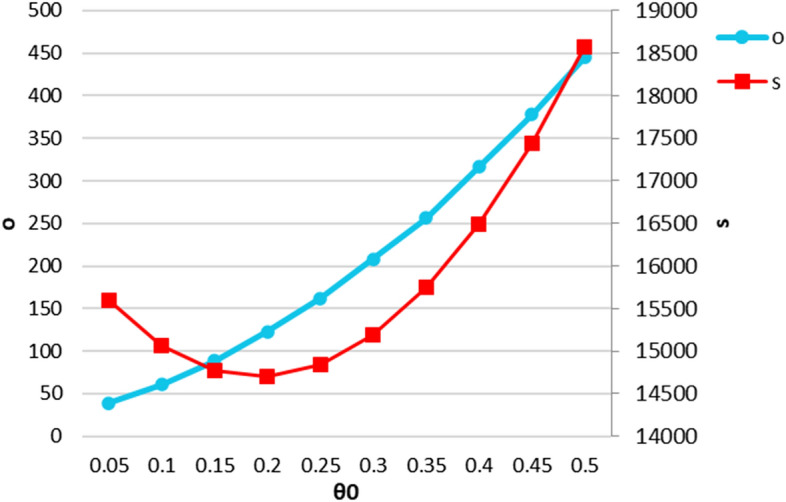
As shown in Fig. 4, as ${\theta }_0$ increases, o increases to compensate for the high perishability of the products. Also, by increasing ${\theta }_0$, the retailer first lowers the price and then raises the price after a ${\theta }_0$ close to 0.2. The retailer in the (${0<\theta }_0<0.2$) range reduces the price to increase the demand. In fact, until ${\theta }_0=0.2$, the deterioration rate has not increased enough that corruption in the warehouse causes excessive damage, but increasing Theta to 0.5 makes more than half of the products in the warehouse corrupted, and to even off this loss, the retailer is forced to increase the price of the products. The NOM also reduces sales efforts because its products price has decreased in the first period, and the demand is high enough. Then, with the increase in product prices and its negative impact on product demand, the NOM increases its sales efforts not to lose its market share.

Fig. 4.

The effect of ${\theta }_0$ on the organic level and sales effort in the decentralized condition

Figure 5 depicts the trend of adjusting the value of ${\theta }_0$ to change the income of chain members. As can be seen from the figures, the change in the profit of the chain members is such that with increasing ${\theta }_0$ the retailer’s profit decreases sharply. This decrease in profit is initially due to the decrease in sales price, but this decrease in profit continues after the increase in prices. With the increase in the rate of product inherent corruption to Theta = 0.5, almost half of NOPs are corrupt. This increase imposes a loss on the retailer that is not offset by an increase in price.

Fig. 5.

The effect of ${\theta }_0$ on profits in the decentralized condition

The NOM’s profit first decreases slightly owing to the fall in the wholesale price of the NOP in this area. However, the profit of this producer increases in the ${\theta }_0>0.2$, owing to the fall in the wholesale price of the product and the increase in demand arising from increased sales efforts.

Also, when ${\theta }_0$ is raised, o rises with a steep slope, and because of the beneficial impact on demand, the OM’s profit rises as well; however, when o is raised, the OM’s operation cost ($\frac{\vartheta o^2}{2}$) rises sharply, and this increase in costs reduces profits. Therefore, by increasing ${\theta }_0$, the organic producer’s profit rises first, then falls.

As shown in Fig. 6, where $\rho$ and ${\theta }_0$ are zero, o is also (tends to be) zero. ${\theta }_0$ depends on the type of product, and it represents the inherent perishability of NOP. Based on the figure, the higher the ${\theta }_0$, the higher the organic level (${\theta }_0$ has a positive correlation with the level of organicity). This is because the organic level covers the impact of the high deterioration rate of the product.

Fig. 6.

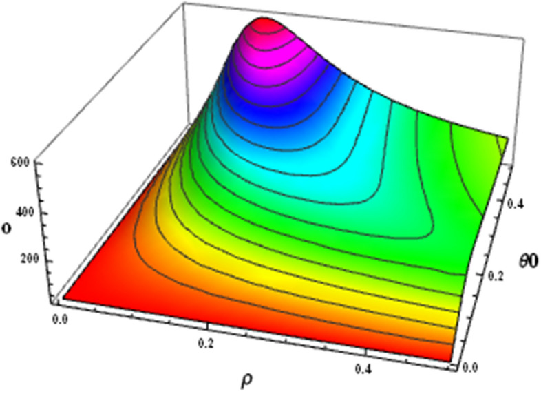
The effect of ${\theta }_0$ and $\rho$ on the organic level in the decentralized condition

In other words, by increasing ${\theta }_0$ in the retail warehouse, more products are corrupted; therefore, the retailer raises the selling price to compensate for this damage, and the OM increases the organic level of the product due to its direct relation with $p_1$. But based on the figure, with increasing $\rho$, the organic level does not increase linearly; It increases up to near $\rho =0.2$ and then decreases. This is because increasing ${\theta }_0$ increases o with a lower slope, but increasing $\rho$ increases o with a steeper slope (the correlation between o and ${\theta }_0$ is less powerful than the correlation between $\rho$ and o), and after a period (interval) when $\rho$ reaches 0.2, o reaches to the high level of itself. According to the profit function of the OM, infrastructure costs for this amount of “o” correlate negatively with the square root of the profit function ($\frac{\vartheta o^2}{2}$) and therefore exceed the profit from selling products, and the OM does not gain profit; For this reason, from that point on, with increasing $\rho$, the organic level decreases so that the manufacturer’s production can be profitable.

As the value of ${\theta }_0$ and $\rho$ increases in the retailer’s warehouse, both OPs and NOPs become more perishable, and the retailer decides to sell the products at a higher price for compensation. Based on Fig. 7, by increasing $\rho$ to 0.2, the increment ratio of the $p_1$ is increased and from this point ($\rho =0.2$), the rate decreases. In fact, $p_1$ is always incremental, but its increment ratio decreases from one point onward. This is because the organic level decreases from that point onward, and since the three decision variables are directly related to each other, decreasing o prevents the price increase sharply and decreases the increment ratio.

Fig. 7.

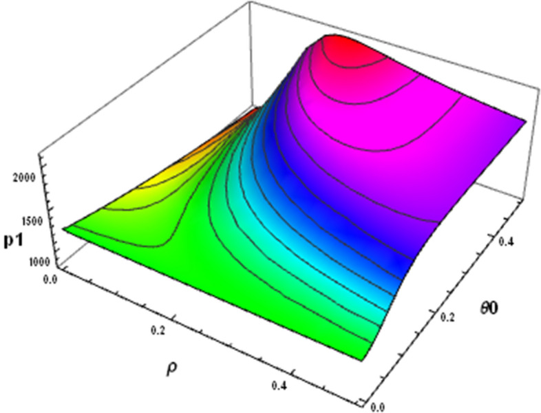
The effect of ${\theta }_0$ and $\rho$ on the OP’s price in the decentralized condition

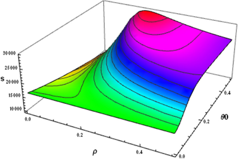
The NOM also increases its sales effort because of the increase in the deterioration rate (${\theta }_0$) caused by the its product price increase. The increase in sales efforts and price is directly proportional. This is because sales efforts compensate for the price increase by the same ratio. It also increases its sales effort by increasing $\rho$ due to increasing o and consequently increasing $p_1$. Increasing $p_1$ also prevents decreasing s after the $\rho$ reaches the point $\rho =0.2$ due to a decrease in o. The correlations between s and ${\theta }_0$ and $\rho$ are shown in Fig. 8.

Fig. 8.

The effect of ${\theta }_0$ and $\rho$ on the level of sales effort in the decentralized condition

Interpretation 2

By summarizing the results of sensitivity analysis, it can be stated that by increasing the inherent corruption of the products of the two manufacturers, they will be more profitable. Due to compensate for the high corruption, they will attempt to sell more and have a higher organic level for their products, which absorbs more demand and higher profit. However, because the retailer will lose large quantities of products in its warehouses in the case of more corruption, it will have less profit by increasing the corruption of the products.

Interpretation 3

According to the mathematical model results and its numerical solution, OMs will have less profit and market share than NOMs. If governments do not support them, they will stop organic production, which will not have good results for the environment.

The government intervention could motivate the manufacturer to produce OPs in the following ways:

• Paying for the investment cost

• Paying for the production cost

• Increasing the market potential of OPs by advertising

• Providing facilities and loans for OMs with lower interest rates

• Exempting OMs from paying taxes

Moreover, many other supports could raise the number of OMs.

To discuss more the interpretations and more specifically present this work’s distinguished contributions, it is necessary to point out that the output of the previous works in the literature focused on the sales efforts or organic level individually, but the results of this paper analyses both the aspects mentioned above simultaneously. Then, it is noticeable to point out certain fruits of the work. First, the competition between sales effort and organic level has been introduced to the literature and clearly explained that organic manufacturing needs more resources and therefore is less profitable, and also OPs have less market share. Second, considering the deterioration rate of the OPs as a function of their organic level and solving the proposed model, and doing the sensitivity analysis to reach the interpretation that with a higher inherent deterioration rate of an OP, the changes in organic level cause severe changes in the chain’s profit was novel in the sense of considering the level of organicity. To wrap this section, most of the novelty in this work was a product of defining the idea of the organic level and adding it to the mathematical model.

Conclusion and future research

Today, the increasing use of preservatives and chemicals in food production has polluted the environment. Also, the chemicals used in food are harmful to human health and will have destructive impacts on the human body. These two reasons have caused concerns for governments and large environmentally friendly producers in recent decades. That’s why we decided to examine the supply chain of OPs and identify the challenges and risks in this chain. In this study, we considered a two-echelon supply chain consisting of two producers and a retailer so that one producer offers OPs with a specific organic level and another producer offers NOPs with sales effort and lower prices than OPs. Both manufacturers sell their products to the retailer, and retailer has both version of products on the shelves of their stores but sell OPs to consumers at a higher price than NOPs. In this supply chain, members of a chain in a Nash game make simultaneous decisions and determine their decision variables. OM determines the organic level; NOM determines the level of the sales effort, and the retailer determines the prices of products. Then the centralized state of the chain is considered, and this time the members of the chain in the Nash game decide on a centralized state. In the case of centralized decision-making, we will have a higher organic level. In fact, in this case, all stages of production and distribution of the product will be organic, and the NOM will have the maximum effort to sell. Also, the overall profit of the chain is higher than the decentralized state. But in centralized decision-making, the OM gets a disadvantage. The retailer shares a proportion of its profit with the OM in a contract to increase the OMs’ profit compared to the decentralized approach and convince him to use the centralized decision-making approach. However, from the results obtained from the real experiment, it can conclude that if a producer decides on producing the OPs, it will significantly have a lower profit than the NOM, and will fail to compete with the NOMs. This failure is due to a couple of reasons. The first reason is the high cost of organic investment, and the second reason is the decrease in OP’s demand due to the increase in its price compared to NOPs. As a result, the organic producer will have a smaller market share.

Finally, several important issues, such as the evaluation of lead-time in the chain and consideration of the stochastic demand for products, remained for future research.

Appendix 1: Proof of Theorem 3.2

Substituting $D_{\mathrm{ri}}$, $Q_{\mathrm{ri}}$, using Taylor Expansion and Eqs. (6), (7), (9), and (10) into Eq. (15), the retailer profit function will be as follows:

$${\pi }_r^d\left({p_1}_{\mathrm{d}}\right)={p_1}_{\mathrm{d}}\left(\alpha ,A,-,\beta ,{p_1}_{\mathrm{d}},+,\lambda ,{p_1}_{\mathrm{d}},\left(1,-,y\right),+,\gamma ,o_{\mathrm{d}},-,\eta ,s_{\mathrm{d}}\right)-w_1\left(\alpha ,A,-,\beta ,{p_1}_{\mathrm{d}},+,\lambda ,{p_1}_{\mathrm{d}},\left(1,-,y\right),+,\gamma ,o_{\mathrm{d}},-,\eta ,s_{\mathrm{d}},+,0.5,T^2,{\theta }_0,\left(1,+,\rho ,o_{\mathrm{d}}\right),\left(\alpha ,A,-,\beta ,{p_1}_{\mathrm{d}},+,\lambda ,{p_1}_{\mathrm{d}},\left(1,-,y\right),+,\gamma ,o_{\mathrm{d}},-,\eta ,s_{\mathrm{d}}\right)\right)+{p_1}_{\mathrm{d}}\left(1,-,y\right)\left(\left(1,-,\alpha \right),A,-,\beta ,{p_1}_{\mathrm{d}},\left(1,-,y\right),+,\lambda ,{p_1}_{\mathrm{d}},+,\phi ,s_d,-,\xi ,o_{\mathrm{d}}\right)-z{p_1}_{\mathrm{d}}\left(1,-,y\right)\left(\left(1,-,\alpha \right),A,-,\beta ,{p_1}_{\mathrm{d}},\left(1,-,y\right),+,\lambda ,{p_1}_{\mathrm{d}},+,\phi ,s_{\mathrm{d}},-,\xi ,o_{\mathrm{d}},+,0.5,T^2,{\theta }_0,\left(\left(1,-,\alpha \right),A,-,\beta ,{p_1}_{\mathrm{d}},\left(1,-,y\right),+,\lambda ,{p_1}_{\mathrm{d}},+,\phi ,s_{\mathrm{d}},-,\xi ,o_{\mathrm{d}}\right)\right)-0.5h{T}^2\left(\alpha ,A,-,\beta ,{p_1}_{\mathrm{d}},+,\lambda ,{p_1}_{\mathrm{d}},\left(1,-,y\right),+,\gamma ,o_{\mathrm{d}},-,\eta ,s_{\mathrm{d}},+,\left(1,-,\alpha \right),A,-,\beta ,{p_1}_{\mathrm{d}},\left(1,-,y\right),+,\lambda ,{p_1}_{\mathrm{d}},+,\phi ,s_{\mathrm{d}},-,\xi ,o_{\mathrm{d}}\right)-0.5c_{\mathrm{d}}{T}^2{\theta }_0(\left(1,+,\rho ,o_{\mathrm{d}}\right)\left(\alpha ,A,-,\beta ,{p_1}_{\mathrm{d}},+,\lambda ,{p_1}_{\mathrm{d}},\left(1,-,y\right),+,\gamma ,o_{\mathrm{d}},-,\eta ,s_{\mathrm{d}}\right)+\left(\left(1,-,\alpha \right),A,-,\beta ,{p_1}_{\mathrm{d}},\left(1,-,y\right),+,\lambda ,{p_1}_{\mathrm{d}},+,\phi ,s_{\mathrm{d}},-,\xi ,o_{\mathrm{d}}\right))$$ 30

The retailer’s profit function will be obtained by calculating the first partial derivatives of ${\pi }_r^d\left({p_1}_d\right)$:

$$\frac{\partial {\pi }_r^d\left({p_1}_d\right)}{\partial {p_1}_d}=A\alpha -{p_1}_d\beta +o_d\gamma -s_d\eta +{p_1}_d(1-y)\lambda +{p_1}_d(1-y)(-(1-y)\beta +\lambda )-{p_1}_d(1-y)z(1+0.5T^2{\theta }_0)(-(1-y)\beta +\lambda )+{p_1}_d(-\beta +(1-y)\lambda )-0.5h{T}^2(-\beta -(1-y)\beta +\lambda +(1-y)\lambda )-w_1(-\beta +(1-y)\lambda )(1+0.5T^2{\theta }_0(1+o_d\rho ))-0.5c_d{T}^2{\theta }_0(-(1-y)\beta +\lambda +(-\beta +(1-y)\lambda )(1+o_d\rho ))+(1-y)(A(1-\alpha )-{p_1}_d(1-y)\beta +{p_1}_d\lambda -o_d\xi +s_d\phi )-(1-y)z(1+0.5T^2{\theta }_0)(A(1-\alpha )-{p_1}_d(1-y)\beta +{p_1}_d\lambda -o_d\xi +s_d\phi )$$ 31

Moreover, by taking the second partial derivatives of ${\pi }_r^d\left({p_1}_d\right)$, the retailer’s profit function will be as follows:

$$\frac{{\partial }^2{\pi }_r^d\left({p_1}_d\right)}{\partial {p_1}_d^2}=-2\beta +2\left(1,-,y\right)\lambda +\left(-,\left(1,-,y\right),\beta ,+,\lambda \right)(1-y)\left(2,-,z,(,2,,+,T^2,{\theta }_0,)\right)$$ 32

To determine the sign of the second derivative of the retailer’s profit function:

• if $z(2+T^2{\theta }_0)>2$ and $\left(1,-,y\right)\beta >\lambda$ and $2\beta >2\left(1,-,y\right)\lambda +\left(-,\left(1,-,y\right),\beta ,+,\lambda \right)(1-y)\left(2,-,z,(,2,,+,T^2,{\theta }_0,)\right)$ the function will be concave.

• if $z(2+T^2{\theta }_0)<2$ and $\left(1,-,y\right)\beta <\lambda$ and $2\beta >2\left(1,-,y\right)\lambda +\left(-,\left(1,-,y\right),\beta ,+,\lambda \right)(1-y)\left(2,-,z,(,2,,+,T^2,{\theta }_0,)\right)$ the function will be concave.

• if $z(2+T^2{\theta }_0)<2$ and $\left(1,-,y\right)\beta >\lambda$ and $2\beta +\left(-,\left(1,-,y\right),\beta ,+,\lambda \right)(1-y)\left(2,-,z,(,2,,+,T^2,{\theta }_0,)\right)>2\left(1,-,y\right)\lambda$ the function will be concave.

• if $z(2+T^2{\theta }_0)>2$ and $\left(1,-,y\right)\beta <\lambda$ and $2\beta +\left(-,\left(1,-,y\right),\beta ,+,\lambda \right)(1-y)\left(2,-,z,(,2,,+,T^2,{\theta }_0,)\right)>2\left(1,-,y\right)\lambda$ the function will be concave.

Appendix 2

By taking the first partial derivatives of Eqs. (11) and (12) the below results are obtained.

$$\frac{\partial {\pi }_{m1}^d\left(o_d\right)}{\partial o_d}=-o_d\vartheta +0.5T^2(-c_1+w_1){\theta }_0(A\alpha -{p_1}_d\beta +o_d\gamma -s_d\eta +{p_1}_d(1-y)\lambda )\rho +(-c_1+w_1)\gamma (1+0.5T^2{\theta }_0(1+o_d\rho ))$$ 33

$$\frac{\partial {\pi }_{m2}^d\left(s_d\right)}{\partial s_d}=(-c_2(1+k{s}_d)+{p_1}_d(1-y)z)(1+0.5T^2{\theta }_0)\phi -c_{2}k(1+0.5T^2{\theta }_0)(A(1-\alpha )-{p_1}_d(1-y)\beta +{p_1}_d\lambda -o_d\xi +s_d\phi )$$ 34

By taking the first partial derivatives of Eq. (19), the below results are obtained.

$$\frac{\partial {\pi }^c\left(o_c,,,{p_1}_c\right)}{\partial o_c}={p_1}_c\gamma -o_c\vartheta -0.5h{T}^2(\gamma -\xi )-{p_1}_c(1-y)\xi +{p_1}_c(1-y)z(1+0.5T^2{\theta }_0)\xi -0.5T^2{w}_1{\theta }_0(A\alpha -{p_1}_c\beta +o_c\gamma -s_c\eta +{p_1}_c(1-y)\lambda )\rho +0.5T^2(w_1-c_1){\theta }_0(A\alpha -{p_1}_c\beta +o_c\gamma -s_c\eta +{p_1}_c(1-y)\lambda )\rho -0.5c_d{T}^2{\theta }_0(-\xi +(A\alpha -{p_1}_c\beta +o_c\gamma -s_c\eta +{p_1}_c(1-y)\lambda )\rho +\gamma (1+o_c\rho ))-w_1\gamma (1+0.5T^2{\theta }_0(1+o_c\rho ))+(w_1-c_1)\gamma (1+0.5T^2{\theta }_0(1+o_c\rho ))$$ 35

$$\frac{\partial {\pi }^c\left(o_c,,,{p_1}_c\right)}{\partial {p_1}_c}=A\alpha -{p_1}_c\beta +o_c\gamma -s_c\eta +{p_1}_c(1-y)\lambda +{p_1}_c(1-y)(-(1-y)\beta +\lambda )-{p_1}_c(1-y)z(1+0.5T^2{\theta }_0)(-(1-y)\beta +\lambda )+{p_1}_c(-\beta +(1-y)\lambda )-0.5h{T}^2(-\beta -(1-y)\beta +\lambda +(1-y)\lambda )-w_1(-\beta +(1-y)\lambda )(1+0.5T^2{\theta }_0(1+o_c\rho ))+(w_1-c_1)(-\beta +(1-y)\lambda )(1+0.5T^2{\theta }_0(1+o_c\rho ))-0.5c_d{T}^2{\theta }_0(-(1-y)\beta +\lambda +(-\beta +(1-y)\lambda )(1+o_c\rho ))+(1-y)(A(1-\alpha )-{p_1}_c(1-y)\beta +{p_1}_c\lambda -o_c\xi +s_c\phi )-(1-y)z(1+0.5T^2{\theta }_0)(A(1-\alpha )-{p_1}_c(1-y)\beta +{p_1}_c\lambda -o_c\xi +s_c\phi )$$ 36

Because the Hessian matrix is a definite negative in this numerical instance, using the second partial derivatives of Eq. (19) reveals that the chain profit function is concave in $o_c$ and ${p_1}_c$ in this real experiment. The partial centralized profit function’s Hessian matrix is as follows:

$$H=\left[\begin{array}{cc}\frac{{\partial }^2{\pi }^c\left(o_c,,,{p_1}_c\right)}{\partial o_c^2}& \frac{{\partial }^2{\pi }^c\left(o_c,,,{p_1}_c\right)}{\partial o_c\partial {p_1}_c}\\ \frac{{\partial }^2{\pi }^c\left(o_c,,,{p_1}_c\right)}{\partial {p_1}_c\partial o_c}& \frac{{\partial }^2{\pi }^c\left(o_c,,,{p_1}_c\right)}{\partial {p_1}_c^2}\end{array}\right]$$

$$\frac{{\partial }^2{\pi }^c\left(o_c,,,{p_1}_c\right)}{\partial o_c^2}=-\vartheta -T^2\gamma {\theta }_0\rho \left(c_d,+,c_1\right)$$ 37

$$\frac{{\partial }^2{\pi }^c\left(o_c,,,{p_1}_c\right)}{\partial {p_1}_c^2}=-2\beta +2\left(1,-,y\right)\lambda +\left(1,-,y\right)\left(-,\left(1,-,y\right),\beta ,+,\lambda \right)\left(2,-,z,(,2,,+,T^2,{\theta }_0,)\right)$$ 38

$$\frac{{\partial }^2{\pi }^c\left(o_c,,,{p_1}_c\right)}{\partial o_c\partial {p_1}_c}=\gamma -(1-y)\xi (1-z(1+0.5T^2{\theta }_0))+0.5T^2{\theta }_0\rho (c_1+c_d)(\beta -(1-y)\lambda )$$ 39

$$\frac{{\partial }^2{\pi }^c\left(o_c,,,{p_1}_c\right)}{\partial {p_1}_c\partial o_c}=\gamma -(1-y)\xi (1-z(1+0.5T^2{\theta }_0))+0.5T^2{\theta }_0\rho (c_1+c_d)(\beta -(1-y)\lambda )$$ 40

For partial centralized profit function to be concave, $\frac{{\partial }^2{\pi }^c\left(o_c,,,{p_1}_c\right)}{\partial o_c^2}$, should be negative, and $\left|H\right|$ should be positive. It is obvious that $\frac{{\partial }^2{\pi }^c\left(o_c,,,{p_1}_c\right)}{\partial o_c^2}=-\vartheta -T^2\gamma {\theta }_0\rho \left(c_d,+,c_1\right)<0$.

Also, if the amount of $\frac{{\partial }^2{\pi }^c\left(o_c,,,{p_1}_c\right)}{\partial {p_1}_c^2}$ be negative, its multiplication in $\left(-,\vartheta ,-,T^2,\gamma ,{\theta }_0,\rho ,(c_d+c_1)\right)<0$ will be positive $\left(\frac{{\partial }^2{\pi }^c\left(o_c,,,{p_1}_c\right)}{\partial o_c\partial {p_1}_c},\times ,\frac{{\partial }^2{\pi }^c\left(o_c,,,{p_1}_c\right)}{\partial {p_1}_c\partial o_c},=,{\left(\frac{{\partial }^2{\pi }^c\left(o_c,,,{p_1}_c\right)}{\partial o_c\partial {p_1}_c}\right)}^2,=,{\left(\frac{{\partial }^2{\pi }^c\left(o_c,,,{p_1}_c\right)}{\partial {p_1}_c\partial o_c}\right)}^2,>,0\right)$ and $\left(\frac{{\partial }^2{\pi }^c\left(o_c,,,{p_1}_c\right)}{\partial o_c^2},\times ,\frac{{\partial }^2{\pi }^c\left(o_c,,,{p_1}_c\right)}{\partial {p_1}_c^2}\right)>{\left(\frac{{\partial }^2{\pi }^c\left(o_c,,,{p_1}_c\right)}{\partial o_c\partial {p_1}_c}\right)}^2$ the determinant of the Hessian matrix will be positive.

In the following conditions, $\frac{{\partial }^2{\pi }^c\left(o_c,,,{p_1}_c\right)}{\partial {p_1}_c^2}$ will be negative:

• if $z(2+T^2{\theta }_0)>2$ and $\left(1,-,y\right)\beta >\lambda$ and $2\beta >2\left(1,-,y\right)\lambda +\left(-,\left(1,-,y\right),\beta ,+,\lambda \right)(1-y)\left(2,-,z,(,2,,+,T^2,{\theta }_0,)\right)$

• if $z(2+T^2{\theta }_0)<2$ and $\left(1,-,y\right)\beta <\lambda$ and $2\beta >2\left(1,-,y\right)\lambda +\left(-,\left(1,-,y\right),\beta ,+,\lambda \right)(1-y)\left(2,-,z,(,2,,+,T^2,{\theta }_0,)\right)$

• if $z(2+T^2{\theta }_0)<2$ and $\left(1,-,y\right)\beta >\lambda$ and $2\beta +\left(-,\left(1,-,y\right),\beta ,+,\lambda \right)(1-y)\left(2,-,z,(,2,,+,T^2,{\theta }_0,)\right)>2\left(1,-,y\right)\lambda$

• if $z(2+T^2{\theta }_0)>2$ and $\left(1,-,y\right)\beta <\lambda$ and $2\beta +\left(-,\left(1,-,y\right),\beta ,+,\lambda \right)(1-y)\left(2,-,z,(,2,,+,T^2,{\theta }_0,)\right)>2\left(1,-,y\right)\lambda$

Data availability statement

Two datasets have been selected from previous research by Zhang et al. (2015) and Bai et al. (2015) in literature and inspired by Mana Company. Data analyzed in this study were a re-analysis of existing data, which are openly available.

References

- Aikaterini M. What motivates consumers to buy organic food in the UK?. Results from a qualitative study. British Food Journal. 2002;104(3–5):345–352. [Google Scholar]
- Asian S, Hafezalkotob A, John JJ. Sharing economy in organic food supply chains: A pathway to sustainable development. International Journal of Production Economics. 2019;218:322–338. doi: 10.1016/j.ijpe.2019.06.010. [DOI] [Google Scholar]
- Bai Q, Chen M, Xu L. Revenue and promotional cost-sharing contract versus two-part tariff contract in coordinating sustainable supply chain systems with deteriorating items. International Journal of Production Economics. 2017;187:85–101. doi: 10.1016/j.ijpe.2017.02.012. [DOI] [Google Scholar]
- Bai Q, Jin M, Xu X. Effects of carbon emission reduction on supply chain coordination with vendor-managed deteriorating product inventory. International Journal of Production Economics. 2019;208:83–99. doi: 10.1016/j.ijpe.2018.11.008. [DOI] [Google Scholar]
- Bai QG, Xu XH, Chen MY, Luo Q. A two-echelon supply chain coordination for deteriorating item with a multi-variable continuous demand function. International Journal of Systems Science: Operations & Logistics. 2015;2(1):49–62. doi: 10.1080/23302674.2014.998314. [DOI] [Google Scholar]
- Cachero-Martínez S. Consumer behaviour towards organic products: The moderating role of environmental concern. Journal of Risk and Financial Management. 2020;13(12):330. doi: 10.3390/jrfm13120330. [DOI] [Google Scholar]
- Carroll P, Pol E, Robertson PL. Classification of Industries by Level of Technology: An Appraisal and some Implications. Prometheus. 2000;18(4):417–436. doi: 10.1080/08109020020008523. [DOI] [Google Scholar]
- Chakraborty T, Chauhan SS, Vidyarthi N. Coordination and competition in a common retailer channel: Wholesale price versus revenue-sharing mechanisms. International Journal of Production Economics. 2015;166:103–118. doi: 10.1016/j.ijpe.2015.04.010. [DOI] [Google Scholar]
- Cohen MA. Joint pricing and ordering policy for exponentially decaying inventory with known demand. Naval Research Logistics Quarterly. 1977;24(2):257–268. doi: 10.1002/nav.3800240205. [DOI] [Google Scholar]
- Fander, A., Yaghoubi, S., & Asl-Najafi, J. (2021). Chemical supply chain coordination based on technology level and lead-time considerations. RAIRO--Operations Research, 55(2). https://www.researchgate.net/publication/349741063_Chemical_supply_chain_coordination_based_on_technology_level_and_lead-time_considerations
- Fander A, Yaghoubi S. Impact of fuel-efficient technology on automotive and fuel supply chain under government intervention: A case study. Applied Mathematical Modelling. 2021;97:771–802. doi: 10.1016/j.apm.2021.04.013. [DOI] [Google Scholar]
- Geetha KV, Udayakumar R. Optimal lot sizing policy for non-instantaneous deteriorating items with price and advertisement dependent demand under partial backlogging. International Journal of Applied and Computational Mathematics. 2016;2(2):171–193. doi: 10.1007/s40819-015-0053-7. [DOI] [Google Scholar]
- Hempel C, Roosen J. The role of life satisfaction and locus of control in changing purchase intentions for organic and local food during the pandemic. Food Quality and Preference. 2022;96:104430. doi: 10.1016/j.foodqual.2021.104430. [DOI] [PMC free article] [PubMed] [Google Scholar]
- Hsiao HI, Kemp RGM, Van der Vorst JGAJ, Omta SO. A classification of logistic outsourcing levels and their impact on service performance: Evidence from the food processing industry. International Journal of Production Economics. 2010;124(1):75–86. doi: 10.1016/j.ijpe.2009.09.010. [DOI] [Google Scholar]
- Hu JY, Zhang J, Mei M, Min Yang W, Shen Q. Quality control of a four-echelon agri-food supply chain with multiple strategies. Information Processing in Agriculture. 2019;6(4):425–437. doi: 10.1016/j.inpa.2019.05.002. [DOI] [Google Scholar]
- Katt F, Meixner O. A systematic review of drivers influencing consumer willingness to pay for organic food. Trends in Food Science & Technology. 2020;100:374–388. doi: 10.1016/j.tifs.2020.04.029. [DOI] [Google Scholar]
- Kotler, P., Armstrong, G., Saunders, J., & Wong, V. (1999). Principles of marketing: 2nd European Edition. Prentice Hall Europe ISBN 978-0-13-262254-7
- Li P, Rao C, Goh M, Yang Z. Pricing strategies and profit coordination under a double echelon green supply chain. Journal of Cleaner Production. 2021;278:123694. doi: 10.1016/j.jclepro.2020.123694. [DOI] [Google Scholar]
- Ma X, Wang S, Islam SM, Liu X. Coordinating a three-echelon fresh agricultural products supply chain considering freshness-keeping effort with asymmetric information. Applied Mathematical Modelling. 2019;67:337–356. doi: 10.1016/j.apm.2018.10.028. [DOI] [Google Scholar]
- Maihami R, Govindan K, Fattahi M. The inventory and pricing decisions in a three-echelon supply chain of deteriorating items under probabilistic environment. Transportation Research Part e: Logistics and Transportation Review. 2019;131:118–138. doi: 10.1016/j.tre.2019.07.005. [DOI] [Google Scholar]
- Mie A, Andersen HR, Gunnarsson S, Kahl J, Kesse-Guyot E, Rembiałkowska E, Grandjean P. Human health implications of organic food and organic agriculture: a comprehensive review. Environmental Health. 2017;16(1):1–22. doi: 10.1186/s12940-017-0315-4. [DOI] [PMC free article] [PubMed] [Google Scholar]
- Molinillo S, Vidal-Branco M, Japutra A. Understanding the drivers of organic foods purchasing of millennials: Evidence from Brazil and Spain. Journal of Retailing and Consumer Services. 2020;52:101926. doi: 10.1016/j.jretconser.2019.101926. [DOI] [Google Scholar]
- Mudgil D, Barak S. Synthetic milk: a threat to Indian dairy industry. Carpathian J Food Sci Technol. 2013;5(1–2):64–8. [Google Scholar]
- Paam P, Berretta R, Heydar M, Middleton RH, García-Flores R, Juliano P. Planning models to optimize the agri-fresh food supply chain for loss minimization: A review. Reference Module in Food Science. 2016 doi: 10.1016/B978-0-08-100596-5.21069-X. [DOI] [Google Scholar]
- Panda S, Modak NM, Cárdenas-Barrón LE. Coordination and benefit sharing in a three-echelon distribution channel with deteriorating product. Computers & Industrial Engineering. 2017;113:630–645. doi: 10.1016/j.cie.2017.09.033. [DOI] [Google Scholar]
- Rana J, Paul J. Consumer behavior and purchase intention for organic food: A review and research agenda. Journal of Retailing and Consumer Services. 2017;38:157–165. doi: 10.1016/j.jretconser.2017.06.004. [DOI] [Google Scholar]
- Ranjan A, Jha JK. Pricing and coordination strategies of a dual-channel supply chain considering green quality and sales effort. Journal of Cleaner Production. 2019;218:409–424. doi: 10.1016/j.jclepro.2019.01.297. [DOI] [Google Scholar]
- Sana SS. Price-sensitive demand for perishable items–an EOQ model. Applied Mathematics and Computation. 2011;217(13):6248–6259. doi: 10.1016/j.amc.2010.12.113. [DOI] [Google Scholar]
- SeyedEsfahani MM, Biazaran M, Gharakhani M. A game theoretic approach to coordinate pricing and vertical co-op advertising in manufacturer–retailer supply chains. European Journal of Operational Research. 2011;211(2):263–273. doi: 10.1016/j.ejor.2010.11.014. [DOI] [Google Scholar]
- Sinha S, Sarmah SP. Single-vendor multi-buyer discount pricing model under stochastic demand environment. Computers & Industrial Engineering. 2010;59(4):945–953. doi: 10.1016/j.cie.2010.09.005. [DOI] [Google Scholar]
- Talwar S, Jabeen F, Tandon A, Sakashita M, Dhir A. What drives willingness to purchase and stated buying behavior toward organic food? A Stimulus–Organism–Behavior–Consequence (SOBC) perspective. Journal of Cleaner Production. 2021;293:125882. doi: 10.1016/j.jclepro.2021.125882. [DOI] [Google Scholar]
- Tayal S, Singh SR, Sharma R. An integrated production inventory model for perishable products with trade credit period and investment in preservation technology. International Journal of Mathematics in Operational Research. 2016;8(2):137–163. doi: 10.1504/IJMOR.2016.074852. [DOI] [Google Scholar]
- Venegas BB, Ventura JA. A two-stage supply chain coordination mechanism considering price sensitive demand and quantity discounts. European Journal of Operational Research. 2018;264(2):524–533. doi: 10.1016/j.ejor.2017.06.030. [DOI] [Google Scholar]
- Viji G, Karthikeyan K. An economic production quantity model for three levels of production with Weibull distribution deterioration and shortage. Ain Shams Engineering Journal. 2018;9(4):1481–1487. doi: 10.1016/j.asej.2016.10.006. [DOI] [Google Scholar]
- Wee HM. Deteriorating inventory model with quantity discount, pricing and partial backordering. International Journal of Production Economics. 1999;59(1–3):511–518. doi: 10.1016/S0925-5273(98)00113-3. [DOI] [Google Scholar]
- Xiao D, Zhou YW, Zhong Y, Xie W. Optimal cooperative advertising and ordering policies for a two-echelon supply chain. Computers & Industrial Engineering. 2019;127:511–519. doi: 10.1016/j.cie.2018.10.038. [DOI] [Google Scholar]
- Xiao T, Xu T. Coordinating price and service level decisions for a supply chain with deteriorating item under vendor managed inventory. International Journal of Production Economics. 2013;145(2):743–752. doi: 10.1016/j.ijpe.2013.06.004. [DOI] [Google Scholar]
- Xie J, Zhang W, Liang L, Xia Y, Yin J, Yang G. The revenue and cost sharing contract of pricing and servicing policies in a dual-channel closed-loop supply chain. Journal of Cleaner Production. 2018;191:361–383. doi: 10.1016/j.jclepro.2018.04.223. [DOI] [Google Scholar]
- Xu X, Zhang M, He P. Coordination of a supply chain with online platform considering delivery time decision. Transportation Research Part e: Logistics and Transportation Review. 2020;141:101990. doi: 10.1016/j.tre.2020.101990. [DOI] [Google Scholar]
- Yan B, Chen X, Cai C, Guan S. Supply chain coordination of fresh agricultural products based on consumer behavior. Computers & Operations Research. 2020;123:105038. doi: 10.1016/j.cor.2020.105038. [DOI] [Google Scholar]
- Yang PC. Pricing strategy for deteriorating items using quantity discount when demand is price sensitive. European Journal of Operational Research. 2004;157(2):389–397. doi: 10.1016/S0377-2217(03)00241-8. [DOI] [Google Scholar]
- Yoo SH. Product quality and return policy in a supply chain under risk aversion of a supplier. International Journal of Production Economics. 2014;154:146–155. doi: 10.1016/j.ijpe.2014.04.012. [DOI] [Google Scholar]
- Zand F, Yaghoubi S, Sadjadi SJ. Impacts of government direct limitation on pricing, greening activities and recycling management in an online to offline closed loop supply chain. Journal of Cleaner Production. 2019;215:1327–1340. doi: 10.1016/j.jclepro.2019.01.067. [DOI] [Google Scholar]
- Zhang J, Liu G, Zhang Q, Bai Z. Coordinating a supply chain for deteriorating items with a revenue sharing and cooperative investment contract. Omega. 2015;56:37–49. doi: 10.1016/j.omega.2015.03.004. [DOI] [Google Scholar]
- Zhang J, Wei Q, Zhang Q, Tang W. Pricing, service and preservation technology investments policy for deteriorating items under common resource constraints. Computers & Industrial Engineering. 2016;95:1–9. doi: 10.1016/j.cie.2016.02.014. [DOI] [Google Scholar]
- Zhang X, Yousaf HAU. Green supply chain coordination considering government intervention, green investment, and customer green preferences in the petroleum industry. Journal of Cleaner Production. 2020;246:118984. doi: 10.1016/j.jclepro.2019.118984. [DOI] [Google Scholar]
- Zhao T, Xu X, Chen Y, Liang L, Yu Y, Wang K. Coordination of a fashion supply chain with demand disruptions. Transportation Research Part e: Logistics and Transportation Review. 2020;134:101838. doi: 10.1016/j.tre.2020.101838. [DOI] [Google Scholar]
Associated Data
This section collects any data citations, data availability statements, or supplementary materials included in this article.