Isotachophoresis: Theory and Microfluidic Applications

Abstract

Isotachophoresis (ITP) is a versatile electrophoretic technique that can be used for sample preconcentration, separation, purification, and mixing, and to control and accelerate chemical reactions. Although the basic technique is nearly a century old and widely used, there is a persistent need for an easily approachable, succinct, and rigorous review of ITP theory and analysis. This is important because the interest and adoption of the technique has grown over the last two decades, especially with its implementation in microfluidics and integration with on-chip chemical and biochemical assays. We here provide a review of ITP theory starting from physicochemical first-principles, including conservation of species, conservation of current, approximation of charge neutrality, pH equilibrium of weak electrolytes, and so-called regulating functions that govern transport dynamics, with a strong emphasis on steady and unsteady transport. We combine these generally applicable (to all types of ITP) theoretical discussions with applications of ITP in the field of microfluidic systems, particularly on-chip biochemical analyses. Our discussion includes principles that govern the ITP focusing of weak and strong electrolytes; ITP dynamics in peak and plateau modes; a review of simulation tools, experimental tools, and detection methods; applications of ITP for on-chip separations and trace analyte manipulation; and design considerations and challenges for microfluidic ITP systems. We conclude with remarks on possible future research directions. The intent of this review is to help make ITP analysis and design principles more accessible to the scientific and engineering communities and to provide a rigorous basis for the increased adoption of ITP in microfluidics.

1. Introduction

1.1. Qualitative Introduction and Definition of Isotachophoresis

We begin with a qualitative description of isotachophoresis (ITP) to frame our summary of its background and development. ITP is an electrophoretic technique useful for the purification, preconcentration, and separation of analytes.^1,2Figure 1 shows a schematic of a simple ITP process, including an arrangement of ions of various types that are migrating due to an applied electric field. This initial basic example of ITP is so-called anionic ITP, where two different anions (and a single common cation) are used to focus anionic samples; however,, as we shall see, ITP can also be performed as cationic ITP (where two cationic species are used to focus cationic samples).

Figure 1.

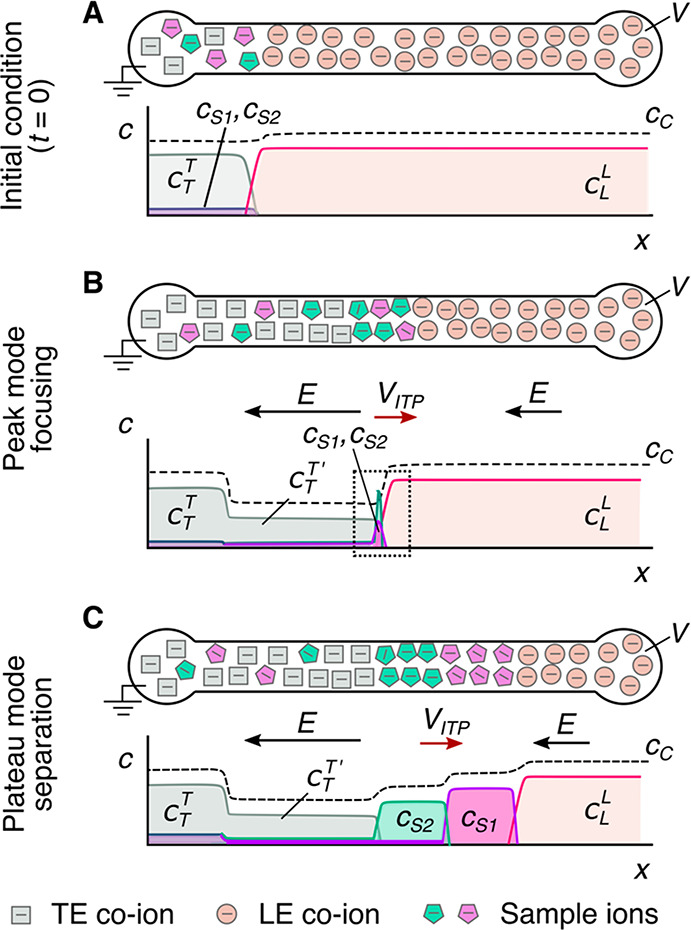
Schematics for the qualitative understanding of microfluidic ITP. (A) Initial conditions at t = 0, common to both peak- and plateau-mode ITP. (B) Peak-mode ITP focusing, which corresponds to either trace analyte focusing or the early stages of any ITP focusing (cf. sections 2.7 and 5). (C) Plateau-mode ITP for the case where the analytes are present in high concentrations and the experiment is run for a sufficiently long duration (cf. sections 2.7 and 6). Each subfigure shows the locations of ions within the channel (top) and the concentration profiles of the electrolytes (bottom) in anionic ITP. For illustration, only two sample species S₁ and S₂ are considered. Peak-mode sample concentration fields are exaggerated for depiction, while sample-mode concentration fields are drawn to relative scale. The loading configuration depicted in panel A, and the schematics in panels B and C correspond to a semi-infinite sample loading configuration (cf. section 2.7).

As shown in the schematic, the system includes an interface between two buffer mixtures. There is a leading electrolyte (LE) mixture and a trailing electrolyte (TE) mixture. These mixtures contain a leading ion and a trailing co-ion (here, anions), respectively. We here define mobility as a proportionally factor between the electric field and the ion drift velocity. The LE and TE anions have relatively high and low magnitudes of mobility, respectively. Upon the application of an electric field, the interface(s) between the LE and TE moves due to electromigration (in the direction opposite that of the electric field). Plotted in the figure are ion concentrations c as a function of the axial dimension along a long-thin channel, x. c_T^T′ and c_L refer to the concentrations of the leading anion. c_T^T refers to the trailing ion concentration in its original location (prior to the application of the electric field), while c_T is the same ion’s concentration in the region that was formerly occupied by the leading ion. As we shall discuss later in this review, c_T^T is a quantity determined by the experimentalist, while c_T is determined by the properties of the LE mixture and the trailing ion mobility. c_C is the concentration of the counterion (here, a cation). The counterion migrates from the LE to the TE zones, and we consider here a single type of counterion in the entire system. Here, E is applied from right to left, and the LE-to-TE interface propagates to the right. We shall see that applying electric field in this orientation (from the TE to the LE) results in a moving self-sharpening interface between the TE and the LE. This sharp moving TE–LE boundary is sometimes referred to as a moving boundary in electrophoresis.³⁻⁵ As we shall see, the self-steepening interface is effectively an ion concentration shock wave whose minimum width is limited by the balance between nonuniform electromigration (established by the electric field gradient) and molecular diffusion.

Further, as we shall see, the relative mobility magnitudes of the LE and TE ions lead to LE and TE regions with high and low ionic conductivity, respectively. This conductivity difference (and the required continuity of the ionic current) necessitates high E in the TE zone, low E in the LE zone, and an electric field gradient at the TE-to-LE interface. This gradient is an essential component required for the selective focusing of sample ions. Sample species whose effective mobilities are greater than the TE ion will, if placed in the TE, migrate faster than the TE co-ion and catch up to and focus at the TE-to-LE interface. Similarly, sample species placed in the LE zone will migrate slower than the surrounding LE co-ion and be caught by and focused into the TE-to-LE interface. In this way, sample ions of a specific mobility range are eventually focused at this interface irrespective of where they are introduced.

The observable concentration and shape of the focused sample ions are a function of their initial concentration and time. As shown in Figure 1b, multiple analyte species initially strongly overlap and focus in the “peak mode” within a small zone. This initial “peak mode” has a local concentration distribution that is a unimodal peak of a magnitude much lower than that of the concentrations of the LE or TE. Given a sufficient initial concentration or sufficient time, analyte species accumulate and increase in concentration to the point where the analyte contributes significantly to the local conductivity. Thereafter, as shown in Figure 1c, an analyte can be purified relative to other co-ions and form a plateau zone that is purified from and displaces its neighboring co-ions. As we shall see, the requirements of current continuity and that the system is approximately net neutral everywhere necessitate a condition wherein locally purified co-ions all migrate at the same velocity despite the fact that they have different mobilities. That is, the co-ions of the LE ion (including the TE ion) and any fully formed plateau travel at the same velocity as the LE ion. Why is this the case? Consider that if the electric field gradients were such that high mobility ions “ran away” from lower mobility ions, the hypothetical gaps formed between co-ionic regions would be regions of unbalanced countercharge (creating internal fields that would act to restore net neutrality). The term “isotachophoresis” refers to the fact that all such zones migrate at the same velocity (the Greek roots “isos” and “tachos” mean equal and velocity, respectively).

As shown in Figure 1c, after multiple plateau zones are formed, the adjacent zones travel as a group at the same velocity as the LE ion. In this configuration, the aforementioned descriptions of the initial TE-to-LE interface as a self-sharpening wave apply to all the newly created interfaces. That is, with respect to the figure, the interface between the LE and sample S₁, the interface between sample S₁ and sample S₂, and the interface between sample S₂ and the TE are all self-sharpening and propagate as a group. The self-sharpening nature of interfaces in ITP makes the separations robust to disturbances, including channel roughness, channel turns, pressure-driven flow disturbances, and modest variations in channel geometry.

Lastly, we briefly note here that orienting an electric field in the “wrong” direction (such that LE ions move toward the TE zone) leads to a phenomenon called electromigration dispersion (EMD). In EMD, the high-mobility ion quickly invades the region occupied by the low-mobility ion, and the low-mobility ion trails back into the high-mobility ion zone (This phenomenon is characterized by an ion migration rarefaction wave).⁶⁻⁹ This situation results in the rapid broadening of interfaces and the associated mixing of co-ionic species. The dispersive nature of EMD is such that it can be easily confused with very rapid diffusion or Taylor dispersion. However, EMD is distinct from these dispersion phenomena as it is a deterministic electromigration-driven mixing phenomenon where, for a constant applied current, interface lengths increase linearly in time (compared to the square root of time expected from diffusion or Taylor dispersion).

1.2. Brief History and Development of ITP

Although the term “isotachophoresis” was introduced only in the 1970s,^10,11 similar techniques based on the principles of ITP have existed for nearly a century. For example, in 1923, Kendall and Crittenden¹² described a technique fundamentally identical to ITP to separate rare earth metals and some acids, which they called the “ion migration method”. Likewise, studies on “moving boundary electrophoresis”,¹³ steady-state stacking in disc electrophoresis,¹⁴ and “displacement electrophoresis”¹⁵ describe processes that are nearly identical (and in some cases identical) to ITP. “Displacement electrophoresis” and “transphoresis” have also been used synonymously with ITP.¹⁶ ITP gained significant popularity in the 1970s as an analytical separation tool that, unlike capillary electrophoresis (CE), could be performed in capillaries with large inner diameters (typically several hundred micrometers) in a stable manner.¹⁷⁻¹⁹ The 1980s saw a decline in ITP’s popularity due to the wide availability of high-quality capillaries with small inner diameters (on the order of tens of micrometers), the easy design of CE buffers, and the high separation performance of CE.^20,21 The early 1990s saw a revival of ITP, but primarily as a tool for preconcentrating analytes and hence as a method of improving the sensitivity of other separation methods, most notably the sensitivities of various CE separation modalities. The earliest form of this type of implementation involved the two-stage on-line coupling of ITP and CE.²² Later, in 1993, this approach was more conveniently implemented via the column-coupling of transient ITP and electrophoresis (mostly zone electrophoresis).²³ See ref (24) for a review of methods of coupling CE and ITP.

The late 1990s marked the first implementations of ITP in a microfluidic format, beginning with the work of Walker et al. in 1998.²⁵ As with many other bioassays, microfluidics offers smaller channel volumes and lower reagent use for ITP. Microfluidics also provides simple optical access and the ability to create on-chip networks that can be accessed and controlled via end-channel reservoirs. Moreover, for ITP, microfluidics offers an on-chip electric field control useful for initiating and terminating electrokinetic processes, switching the electric field direction among intersections (e.g., for mixing) and bifurcations (e.g., for aliquoting) within on-chip networks, and, in the case of glass or fused silica, a relatively efficient heat sink to mitigate the effects of Joule heating as a result of ITP. Consistent with and following the successes of capillary ITP–CE systems, initial applications of microfluidic ITP in the late 1990s and early 2000s combined on-chip transient ITP preconcentration with zone electrophoresis.²⁶⁻³⁰ Later in the 2000s, other on-chip applications for ITP were developed, including sample purification and preconcentration,^31,32 sample focusing and separation,³³⁻³⁷ and control and acceleration of biochemical reactions.^38,39 Over the last two decades, ITP has enjoyed increased adoption and growing interest in microfluidic formats due to its ease of adaptability and compatibility with miniaturized devices. Currently, around 200 papers are published each year that describe developments or applications of microfluidic isotachophoresis across various disciplines, including chemistry, engineering, molecular biology, materials science, and environmental science (based on data from Scopus as of 2022).

The theory and physicochemical principles of ITP have been addressed in a classic book and several book chapters. Perhaps the most influential of these theory reviews is the book by Everaerts et al.¹ titled “Isotachophoresis”. Everaerts et al. presented models of ITP ion mobility and migration dynamics. Their descriptions were confined mostly to simple algebraic relations for the coupling of pH equilibrium, electroneutrality, mass balances, and current conservation (at steady state), and they discussed only qualitatively unsteady dynamics, including the development and growth of plateau zones. Coxon and Binder¹⁶ presented 1D conservation (partial differential) equations that led to analytical solutions (including steady interface distributions) and a confirmation of the Kohlrausch regulating function, but unfortunately their work is limited to strong electrolytes. In the chapter “Analytical Isotachophoresis”, Boček² presented formulas for the dynamics of strong electrolytes and only summarized some classic results of weak-electrolyte plateau concentrations by Svensson⁴⁰ and Dismukes and Alberty.⁴¹ Boček covered the analytical solution for the steady-state distribution at the interface of two neighboring plateau co-ions.² Boček also presented formulas for the separation capacity and expert discussions of practical aspects, including the detection of plateaus with temperature, the mitigation of Joule heating, counterflow ITP, and separation assays that used plateau-mode ITP. Subsequently, Krivankova et al.⁴² published a book chapter covering ITP that offered very good and practical advice for buffer and experimental setup designs (including column coupling) and interesting application examples but very little by the way of theoretical development (aside from stating the so-called ITP condition). Despite all these texts, we know of no summary of ITP physics that both summarize the derivations of the Alberty and Jovin functions and formulates the dynamics of ITP processes. The current review also uniquely includes a summary of unsteady ITP ion concentration fields starting from first-principles (including species and current conservations, the electroneutrality approximation, and chemical equilibrium). Unlike past reviews, the current review also covers details of peak-mode ITP, including accumulation rates and peak distributions.

In accordance with the very strong interest in ITP, a good number of review articles addressing various aspects of ITP have been published over the last 20 years.^{43,44,53−58,45−52} The majority of these are articles on ITP were published periodically and incrementally, covering developments in instrumentation, experimental techniques, modeling, and simulation for both capillary and microfluidic ITP systems. The latter reviews typically cover progress over a few years at a time (most commonly, periods of two years). To our knowledge, the first article that exclusively reviewed microfluidic ITP was the work of Chen et al.²⁶ in 2006. This work largely focused on developments in microchip-based technologies between 1998 and 2006 for the ITP-based analysis and pretreatment of biomolecules and ionic compounds. We know of only one other broad review article on microfluidic ITP, which was published by Smejkal et al.¹⁹ in 2013. This article primarily discussed applications of microfluidic ITP and placed scant emphasis on discussions of theoretical principles, analysis, or assay design. The field of microfluidic ITP has significantly evolved since the article of Smejkal et al., and there have been many new developments in both theoretical aspects and the fundamental understanding of ITP (e.g., sample zone dynamics, dispersion in peak-mode ITP, and ITP-aided reactions)^{38,39,59−62} in addition to new applications (e.g., single-cell analyses and ITP-aided reactions).^38,63,64 Several topical reviews have focused on various subfields of microfluidic ITP over the past decade. For example, in 2013, Bahga and Santiago²⁴ reviewed in detail the coupling of microfluidic ITP with zone electrophoresis. The application of ITP to nucleic acid sample preparation, including purification and preconcentration, was reviewed by Rogacs et al.³¹ in 2014 and later by Datinská et al in 2017.⁶⁵ In 2018, Eid and Santiago³⁸ reviewed applications of ITP to biomolecular reactions. Recently, in 2020, Khnouf and Han⁶⁶ reviewed challenges and opportunities for ITP-based immunoassays. Despite several such examples, no review article broadly covers all aspects of microfluidic ITP systems, including theory, applications, experimental tools, detection methods, practical considerations for system design, and limitations. For example, we know of no succinct and rigorous (in any format, including review papers or textbooks) that attempts to present a review of the physicochemical fundamentals of ITP dynamics starting from first principles. In fact, we believe that the lack of any such quantitative review of the physics and chemistry has inhibited the adoption and spread of ITP as a technique in any format (traditional or microfluidic). We therefore believe that such a review is timely and has the potential to strongly influence the rapidly growing research field of microfluidic ITP.

1.3. Overview of This Review

We here provide an overall review of microfluidic ITP systems starting from first principles, with a strong focus on the description of fundamental physicochemistry of ITP. We combine this fairly general introduction to the theory of ITP with a review of the emerging applications of, specifically, microfluidic ITP systems. Accordingly, most applications reviewed in this work are from studies published within the last two decades, and we particularly emphasize microfluidic ITP applications that involve biological analyses. In section 2, we begin by reviewing key conservation principles and terminology useful in the analysis of ITP systems. We also provide a brief review of chemical buffers and general electrophoresis principles for weak electrolyte systems ,including the concept of effective mobility, and discuss configurations of sample loading strategies and ITP modes (peak versus plateau). Next, in section 3, we review the theory for ITP processes for strong electrolytes, including derivations of the Kohlrausch regulating function and analytical expressions for the concentration of a focused sample and LE-to-TE interface width. Later, in section 4, we review the theory for the ITP of weak electrolytes, including derivations of the Jovin and Alberty regulating functions. Later, we discuss the theory for the identification of trace analytes in peak-mode ITP and the separation process in plateau-mode ITP in sections 5 and 6. As part of sections 5 and 6, we review the theory for estimation of analyte accumulation rates, zone lengths for the plateau mode, and sample zone dynamics for the peak mode. In section 7, we review the theory and various models for systems in which ITP is used to initiate, control, and accelerate both homogeneous and heterogeneous chemical reactions. We subsequently review several practical considerations and limitations of microfluidic ITP systems in section 8, including dispersion, Joule heating effects, buffering, separation capacity, operation method, sample volume versus sensitivity trade-off, and channel materials. In section 9, we summarize publicly available simulation tools useful for modeling and studying ITP systems. In section 10, we review various experimental tools and methods for analyte detection that are compatible with microfluidic ITP and provide scaling arguments around sensitivity and resolution for the detection of plateau zones. In section 11, we provide an overview of several types of systems that leverage ITP for trace analyte detection and separations, including bioassay systems that involve nucleic acids, proteins, and single cell analyses. Then, in section 12, we provide a brief overview of miscellaneous techniques used in microfluidic ITP, including the coupling of ITP preconcentration with zone electrophoresis, cascade ITP, counter-flow and gradient elution ITP, and free-flow ITP. Lastly, in section 13, we conclude with remarks on possible future research directions for microfluidic ITP.

2. Basic Concepts and Terminology

In this section, we first define the mobility of an ion under an applied electric field and briefly discuss the basic terminology and notation we use to describe such ions and ion families. Refer to Supporting Information Table S1 for a detailed nomenclature list, including variable names, brief descriptions, and units. Our discussions in this section involve both strong and weak electrolytes, which respectively refer to fully ionized and partially ionized species. We review steady and unsteady transport phenomena starting from physicochemical first-principles, including the conservation of species, the conservation of current, and the approximation of charge neutrality. These concepts are generally applicable to all electrophoresis systems and, more specifically, are useful for describing systems over the relevant length and time scales involved in ITP. We then briefly review the pH equilibrium and electrophoresis of weak electrolytes, including a discussion around the total concentration and effective mobility of a weak electrolyte. We then describe two useful approximations of safe and moderate pH conditions, which we will use in subsequent sections to simplify ITP analyses. We conclude this section with qualitative descriptions of various ITP modalities, including strong versus weak electrolyte ITP, finite versus semi-infinite sample injection, and peak- versus plateau-mode ITP.

2.1. Ion Mobility and Ion Families

Our discussions of ITP will require descriptions of multispecies systems that change in space and time, and so we begin by describing our notation for ion mobility and concentration and presenting some basic physicochemical relations. Our notation is designed to simplify descriptions of ITP systems, including weak electrolytes (which require the additional specification of mobilities and the local ionization state; see below). First, we describe our definition and the associated dimensions of ion mobility (a.k.a. electrophoretic mobility). Our basic definition of ion mobility shall be simply the ratio of the ion drift velocity divided by the local electric field. The drift velocity will, of course, be measured as the velocity of the ion relative to that of the local continuum fluid of the aqueous solvent. The dimensions of this mobility are then the square of a length per unit of electric potential and time. In the SI system, the units of our mobility definition will be meters squared per volt per second (m² V^–1 s^–1). We shall use the symbol μ for mobility and use subscripts to distinguish among ion types and properties. For example, the relation among the mobility of ion i with (integer-valued) valence z, its drift velocity vector u̅_i,z and the local applied electric field E̅ is u̅_i,z = u_i,zE̅.

In ITP systems, there is often some finite region in space where the chemistry is locally uniform. The most common of example of this is the LE zone, but locally uniform properties can also exist within trailing and plateau zones.

First, the quantities μ_A,z^X and c_A,z refer respectively to the fully dissociated electrophoretic mobility (a signed quantity) and the concentration of the species with a specific valence z that is a member of some ion family A. Here, the ion family is defined as all species within a particular chemical group with the ability to donate or accept protons. For example, A can refer to all ionic forms of the aqueous phosphoric acid “family”, e.g., PO₄^3–, HPO₄^2–, H₂PO₄^–, or H₃PO₄, that have respective ionization states z equal to −3, −2, −1, and 0 (cf. section 2.4). The superscript X refers to the zone of interest (i.e., a location in space, at a specific time). Examples of zones include the leading electrolyte zone, the trailing electrolyte zone, or some generic plateau zone. We next describe our notation for strong and weak electrolytes. Recall that a strong electrolyte refers to a solution where all the solute species are fully ionized (e.g., NaCl), while a weak electrolyte refers to a solution where the solute species are only partially ionized (cf., section 2.4). For strong electrolytes, we omit the superscript in the mobility since the mobility of a fully ionized electrolyte is independent of the zone. The presence of a superscript in the mobility refers to the description of a weak electrolyte, whose mobility can vary depending on the degree of dissociation and the zone of interest. Note that the superscript in the mobility is redundant when describing fully ionized electrolytes. Superscripts can always be used for concentration, since concentrations in ITP vary in space and time (cf. section 2.2). Next, since the mobility of weak electrolyte ions is a function of the local pH and the various ionization states, we need to describe an “effective” mobility for such a species family that will account for all the relevant ionization states of A (see the formal discussion in section 2.5). We will denote the effective mobility of A with an overbar as μ̅_A^X. Note this overbar can never be confused with vector notation as mobility is always a scalar. Likewise, we use the notation c_A (i.e., the lack of a second subscript) to denote the total concentration (a.k.a. the analytical concentration) of A across all ionization states. For example, the total concentration of the phosphoric acid family described earlier is c_A = c_A,–3 + c_A,_–1 + c_A,–2 + c_A,0. Concentrations of strong electrolytes, of course, require only one specified or implied (e.g., unwritten) subscript (since there is only one relevant ionization state).

2.2. Basic Conservation and Transport Relations

We here introduce basic conservation principles, including ion transport and current. For simplicity, we will assume ionic solutions that are sufficiently dilute to apply the well-known Nernst–Planck⁶⁷ for the vector flux J̅ (mol m^–2 s^–1) of ion i with valence z.

1

Here, c_i,z is the ion’s concentration (in molar density units), D_i,z is a molecular diffusivity, and u̅_b is the bulk fluid (i.e., solvent) velocity. Note further that the mobility μ_i,z can be related to the diffusivity according to the Nernst–Einstein relation⁶⁸ given by μ_i,z = zD_i,zF/RT, where R is the universal gas constant, F is the Faraday constant, and T is the absolute temperature. From the relation in eq 1, we can derive a general relation for the conservation of species over a differential control volume of the fluid. This derivation can be found in several classic references; for interested readers, we here recommend the textbooks of Probstein⁶⁷ and Deen.⁶⁹ The resulting conservation equation is

2

where R_i,z is the production rate and area-averaged concentration of species i (valence z) (i.e., due to chemical reactions). For this conservation of a dilute ion, we assume that the solvent is an incompressible liquid such that ∇·u̅_b = 0. The latter equation is useful in the study of a large number of electrokinetic systems. For simplicity, and as a simple introduction to ITP dynamics, in this section we consider the very simple case of one-dimensional transport and a negligible bulk fluid velocity. Under these assumptions, we derive the following:

3

Here, x is the streamwise direction along a channel. We will consider all aspects and terms of this equation in our description of ITP, so it is worth reviewing this expression and building intuitions for their coupling. For example, we shall typically consider uniform values of diffusivity and mobility for any specific ion. Importantly, the equation nevertheless includes the product c_i,zE, which makes it nonlinear. We shall see that it is this term that can result in the shock and rarefaction wave behavior of ion transport. We shall also consider cases where the reaction term is very significant, including cases of chemical equilibrium (cf. section 4) and unsteady chemical kinetics (cf. section 7).

We next describe the important concept of current density in multi-ion systems, which we will then use (in section 2.3) in our discussion of current conservation. Again, assuming one-dimensional transport and a negligible bulk current, the Nernst–Planck flux reduces to . If we multiply this relation by the valence z of each ion type and the Faraday constant F and then sum over all ionic species, we naturally derive the following expression for the current density j:

4

From this summation, we see that we inherently formulate the Ohmic conductivity, σ, of these mixture as follows:

5

Here, the double summation implies summations across the various ionization states within each family and across all species families (i = 1 to N). The bounds n_i and p_i are, respectively, the most-negative and most-positive valence states within each species family. For example, for an ampholyte that can, in some relevant pH range, acquire valence states −1, 0, and 1, n_i and p_i are, respectively, −1 and 1. Importantly, the expression for the current density demonstrates an important consequence of the Nernst–Planck relations above. Namely, we see that current can be transported not only by ion mobility (Ohmic-type transport) but by diffusion.⁶⁷ Note that neglecting of the bulk velocity in the formula for the current is typically a good approximation for typical electrokinetic systems where the ionic strength is sufficient such that charge relaxation times are much shorter than the characteristic advection times.^70,71

In subsequent sections, we will discuss in more detail the applications of the conservation of species and current. For now, we note simply that, away from regions of sharp interfaces (i.e., high diffusion gradients), such as the interface between ITP zones, we can assume that the current density is given simply by the Ohmic current, j ≈ σE. An important consequence of this is that regions of low conductivity necessarily imply a high local electric field, and vice versa. This approximation provides additional insight into the qualitative discussion of section 1.1 above.

We conclude this section by listing the results for species conservation and the current for the simpler case of a strong electrolyte (i.e., a species with uniform and constant valences and no chemical reactions). For this case, our species conservation reduces to

6

Despite the severe simplifications, we see that the aforementioned nonlinearity remains, which is an essential feature of ITP. Lastly, the expression for current density j summed over i = 1 to N strong electrolytes is then

7

where the ionic conductivity σ (from eq 5) is simply σ = F ∑_i = 1^Nz_iμ_ic_i.

2.3. Charge Neutrality Approximation and Divergence of Current

We here introduce the powerful approximation of electroneutrality (a.k.a. charge neutrality) for electrokinetic systems. In ITP, we shall use electroneutrality to formulate the dynamics that lead to the equal electromigration velocities of the LE and TE zones (cf. section 3.1). Persat and Santiago⁷² describe scaling arguments, which originate from the Gauss law for diffuse ion systems, that lead to the electroneutrality assumption as well as the so-called Ohmic model for electrokinetics (see also refs (73) and (74)). We here present a similar scaling argument in the context of ITP. We consider a region subject to some electric field that is imposed by electrodes placed far from this region (e.g., at end-channel reservoirs). These electrodes have a sufficient potential difference to sustain Faraday reactions and hence force a net ionic current through the system, including our region of interest. The region has an approximately uniform permittivity, ε (e.g., dominated by the polarizability of water under approximately isothermal conditions), but has significant gradients in species concentration (and therefore ionic conductivity, as per eq 5). The general result is a spatially varied electric field E̅ within this region. The differential form of the Gauss law then relates the gradients of this electric field to any net charge density as follows:

8

The right side of this equation is the net charge density, ρ_E, expressed here in terms of ion concentrations for some arbitrary mixture of weak electrolytes (summed over i = 1 to N species families, each of which has valence states between n_i and p_i). F is the Faraday constant. Without a loss of generality, we can decompose the local electric field into external and internal components as follows: E̅ = E̅_ext + E̅_int. We define E̅_ext as the nominal applied electric field that would result from the electrodes if the species concentrations and properties were uniform such that ∇·E̅_ext = 0. Hence, E̅_int is the electric field component that results strictly from the net charge and associated species gradients. Figure 2 depicts the situation in the context of a one-dimensional treatment of an ITP interface. We analyze species gradients over some diffuse interface of length scale δ. Sufficiently far from the interface, regions L and T have locally uniform species concentrations and ionic conductivities σ^L and σ^T and hence locally uniform current densities σ^LE^L and σ^TE^T, respectively (cf. eq 4). Here, E^L and E^T are the local electric fields in the L and T regions, respectively. We will discuss current conservation later in this section and show that, to a high degree of approximation, σ^LE^L ≅ σ^TE^T, even for typical unsteady ITP processes. Hence, under quasi-steady conditions, conservation of current demands that E^L and E^T be different; hence, there must be (from Gauss’ law) a net charge within the interface. As we discuss below, the net charge within the interface and the sharp gradient in the electric field are associated with an internally generated electric field E̅_int, which is directed away from the interface.

Figure 2.

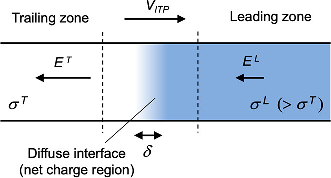
Simple one-dimensional treatment of an ITP interface. The diffuse interface between the two region has a length scale δ. The regions away from the interface have locally uniform conductivities σ^L and σ^T. Current conservation requires a sharp gradient in the electric field and therefore a local net charge.

Given this situation of a one-dimensional monotonic gradient in conductivity, we can bound the scale of E_int. In ITP, typical values of the high-to-low conductivity ratio σ^L/σ^T are roughly a factor two or less. Hence, we expect that, at most, the electric field between the regions will change by a factor of two or less such that E_int is on the order of E_ext. Even for some extreme case where σ^L/σ^T is on the order order of 20, E_int will remain on the order E_ext so long as the region occupying the lower conductivity has an axial length that is on order of the total length between electrodes. We can now proceed with our scaling analysis. We scale the left side of eq 8 as εE_int/δ) (where E_int ≈ E_ext). For the purpose of scaling, we also simplify the right side for the case of strong monovalent electrolytes, obtaining

9

where N_cat and N_ani are, respectively, the local number of (monovalent) cationic and anionic species (and N = N_cat + N_ani). Next, the dimensional parameters c₊ and c_– as the (local) are defined as the characteristic sums of cations and anions, respectively. Additionally, we define c_o as the characteristic sum of the concentrations of all (monovalent) ionic species, c_o = ∑_i = 1^Nc_i, and write

10

We thereby define the parameter α as a measure of the characteristic difference in concentration between positive and negative charges relative to the characteristic background concentration of all ionic species. We can estimate α for typical ITP systems as follows. Empirically, we observe that ITP systems exhibit interfaces with minimum diffusion-limited lengths of roughly 10 μm. Externally applied fields are at most order 10⁴ V m^–1 (and hence E_int is on the order of 10⁴ V m^–1). Due to pH buffering considerations (cf. section 8.4), minimum practical values of c_o are on the order of 1 mM. Substituting these dimensional scales into eq 10, we see for aqueous solutions that α has a maximum of roughly 10^–5 (see also ref (72)). That is, a very small mismatch between the concentrations of the cations and anions is enough to account for internally generated electric fields in ITP. This tiny mismatch is very important in conserving the electric flux but, for the purposes of conserving species and applying eq 3, we assume the system is approximately net-neutral. Hence, at any position and time, the concentrations of negative and positive charges are assumed to be equal for the purpose of computing the transport of local ion concentrations (via the conservation of species relations). This is the essence of the electroneutrality approximation.

We shall leverage the net-neutrality approximation in our equations of both ion transport and chemical equilibrium. Basically, we will assume (to a high degree of accuracy) that, any position and time, the concentrations of negative and positive charges are equal when local ion concentrations are computed using transport principles and expressions of chemical equilibria. For example, for a univalent three-ion ITP system consisting of a TE co-ion, a LE co-ion, and a common counterion (e.g., see Figure 1 and assume no sample ions), charge neutrality in the adjusted TE region implies that c_C^T′ + c_H = c_T + c_OH.

A second concept that arises from the electroneutrality is the so-called Ohmic model of electrokinetics,⁷² which is how we compute electric fields in the system. A rigorous and exact computation of electric fields generally requires a careful computation of the unsteady net-charge fields in the system (particularly at conductivity interfaces) via careful balances of the Gauss law in addition to all species conservations. However, for most electrokinetic systems, we can finesse the electric field calculation with a different approach. Namely, we can assume quasi-steady charge accumulation^72,75 (a.k.a. the relaxed charge approximation) and electroneutrality whenever we compute the species conservation. We then compute electric fields from the conservation of current. In ITP, this approach is especially useful to obtain closed-form solutions for ion concentrations at points within plateau regions or in control volume analyses of ITP ion fluxes. A fully three-dimensional version of eq 7 yields a more general description of the current density flux for multispecies weak electrolyte electrokinetic systems as follows:

11

Using this expression of the current flux, the conservation of net charge density ρ_E over a differential element yields⁶⁷

12

We next apply the approximation of relaxed charge, which assumes that the time scale for the accumulation of the net charge (as in the net charge region in the diffuse interface shown as an example in Figure 2 above) is much smaller than the time scale of interest.^72,75 In electrokinetic systems, the latter time scales are typically milliseconds or less. For this regime, we have simply

13

This equation can be interpreted as a form of Kirchoff’s law but is in fact a more general expression, since it includes contributions of diffusive fluxes to current transport (cf. eq 4). It is valid for unsteady processes whose characteristic time scales are significantly larger than the charge relaxation time scale of the system. A useful form of this equation can be derived by simply integrating over a finite volume and applying the divergence theorem to obtain

14

where CS refers to a (closed) integral over a control surface. This three-dimensional form is useful, as it can be applied over complex volumes that span intersections among an arbitrary number of channels (e.g., as in microfluidic systems). For control volumes whose control surfaces are drawn far from sharp concentration gradients (e.g., away from an LE–TE interface) or at the wall–liquid interface, this expression for the conservation of current reduces to a traditional Kirchoff’s law expressed in terms of the Ohmic current as follows:

15

We saw an example of this concept in the scaling argument presented at the beginning of this section. In that example, our control volume yielded σ^LE^L ≅ σ^TE^T.

The net-neutrality approximation will also be useful in analyses of both chemical equilibrium and transport phenomena associated with ITP. We conclude this section with the following example formula for the net-neutrality approximation of a weak electrolyte mixture:

16

Here c_H and c_OH are the concentrations of the hydronium and hydroxyl ions, respectively. In this way, we will treat these ions (associated with the autoprotolysis of water) separately from the species families of interest. Note that protons (or more exactly hydronium ions) and hydroxyl ions are always of critical importance in weak electrolyte systems due to the strong pH-dependence of the species mobility.

2.4. Brief Review of pH Buffers

Before we continue with our discussion of the ITP of weak electrolyte systems, it is instructive to briefly review the concept of a chemical buffer. A detailed review of buffers and the electrophoretic transport of weak electrolytes can be found in refs (76) and (77). We shall assume here a working knowledge of these topics and adapt the Brønsted–Lowry definition of acids and bases (as, respectively, proton donors and acceptors). We will emphasize the case of anionic ITP systems wherein the TE and LE co-ions are (strong or weak acid) anions and the common counterion is a weak base used to provide a pH buff for the ITP system.

Consider a buffer created using a singly ionized weak base and a strong acid, such as HCl. The (proton exchange) chemical equilibrium reactions are

17

Here, we use “B” to denote a generic Brønsted–Lowry weak base, that is, a proton acceptor. To achieve pH buffering in this mixture, the weak base is obviously the “buffering species” and the chloride ion (here, from the strong acid) is the “titrant”. Note that we present reactions with the proton species on the right side, as this facilitates bookkeeping among a significant number of species and the coupling of simulations with large databases of the properties of weak acid species.⁷⁶⁻⁷⁸ The latter arrangement of species in the reactions in eq 17 also allows us to specify all dissociation constants, K, as the appropriate acid dissociation constants, K_a. Henceforth, we will drop the “a” in the subscript of K_a where appropriate, with the understanding that K refers to the acid dissociation constants. We instead use the subscripts of K to indicate the species family and the ionization state. The two equilibrium reactions and mass conservation relations for eq 17 are then

18

where c_B,tot and c_B,tot are, respectively, the total amounts of (generic) base B and strong acid HCI initially added to the mixture. The definitions of the other concentration variables follow from our discussions of section 2.1 (i.e., c_B,0 refers to the concentration of the weak base B, and c_B,1 refers to the concentration of the corresponding conjugate acid BH⁺). From charge neutrality, we have

19

Though it is possible to solve these equations as-is (by solving a parabolic equation with the concentration of hydronium as the root), the assumption of moderate pH (i.e., anticipating a resulting pH between about 4 and 10, see section 2.6) is a useful simplification, allowing us to rewrite eq 19 as c_B,1 ≈ c_Cl = c_HCl,tot. Combining these equations, we derive

20

and

21

Here, pH = −log₁₀ H⁺, pK_B,0 = −log₁₀K_B,0, and c_HCl,tot = c_Cl,tot. For a well-designed classic buffer, the pH is near the pK_a of the weak electrolyte. The strongest buffering capacity condition is achieved when pH = pK_B,0 or, equivalently, c_H = K_B,0. Further, pH = pK_B,0 implies c_BH⁺,tot = 2c_HCl,tot. We see the strongest buffering capacity when buffering species are half-dissociated by the ionized concentration of the (typically fully ionized) titrant.

Similar analyses can be performed for a variety of cases, including fairly arbitrary mixtures of weak and strong acids and weak and strong bases or salts. Refer to Persat et al.⁷⁶ for details.

2.5. Electrophoresis of Weak Electrolytes

We review concepts around the electromigration of mixtures comprised of weak electrolytes. In such systems, typical acid–base chemical equilibrium reaction kinetics occur over a much smaller time scale than characteristic advection and diffusion time scales.⁷⁹ Hence, we will here assume that each species is in chemical equilibrium at all times. See refs (80) and (81) for examples where finite reaction kinetics may be important in ITP.

2.5.1. Total Concentration, Species Conservation, And Effective Mobility

For weak electrolyte solutions, the conservation of species requires that the sum the total of members of each chemical “family” be conserved. To show this, we define this sum across members of a chemical family as the total (a.k.a. analytical) concentration of “family” i.

22

The total concentration of buffer species is typically a known quantity. For example, this quantity may be determined by weighing some amount of a weak base stock-supply powder. Alternately, the quantity is known from a dilution of a stock solution of the electrolyte. Further, since the various members of a single family can only accept or donate protons, the sum of the various production rates in the species conservation equation (eq 3) across the family, ∑_z = ni^piR_i,z, is identically zero. Summing the weak electrolyte conservation equation across the members of a single family, we can eliminate the production term and obtain a simplified conservation equation for the total concentration c_i as follows:

23

Further, assuming that all the members of family i have a similar diffusivity D_i for simplicity, we can write

24

The resulting relation for the net transport of each species family has a strong similarity to the conservation equation for fully ionized species. The important difference here (compared to eq 6) is that we have formulated the relation in terms of a total concentration and defined a new quantity μ̅_i as the effective mobility of family i. This effective mobility describes the net rate of migration of all members of the family in terms of the absolute mobilities μ_i,z of the individual species of the family weighted by the molar fraction of the species within the family. μ̅_i is given by^79,82

25

Interestingly, the modified conservation equation for the total concentration (eqs 23 and 24) describes the net transport of a group of species that are created and destroyed by acquiring and donating protons, respectively, but the equation contains no explicit reaction term. The physicochemistry of the acid–base reactions that is embedded into the chemical equilibrium determines the various values of species concentrations c_i,z and, of course, the concerted interactions of all the families determine the local and instantaneous pH.

2.5.2. Effective Mobility: An Example Calculation

To illustrate the procedure for calculating the effective mobility of a species family, we here consider the example of a singly ionized weak acid electrolyte A (e.g., an analyte in anionic ITP). The equilibrium reaction for A is given by A ⇌ A^– + H ⁺. The associated equilibrium reaction and species conservation relations can be written as

26

where c_A,tot is the total (or analytical) concentration.

In the ideal limit when the conjugate base ion A^– is fully dissociated at z = −1 (and the effects of ionic strength on ion mobility and dissosciation constants are neglected⁷⁷), the electromigrative drift velocity u_A^– of ion A^– can be written in terms of its absolute mobility μ_A,–1 as u_A^– = μ_A,–1E. However, more generally, the observed drift velocity of the species family is described by the effective mobility, which accounts for the time-averaged velocity of species A as it accepts and donates protons. This effective mobility is defined by the relation

27

where

28

and K_A,–1 is the acid dissociation constant. The overbar here denotes the average mobility observed for this species family. The species quickly acquires and donates a proton, but this process is so fast that we observe only the species’ time-averaged mobility.

Consider two example buffer conditions for eq 28. First, for a well-designed buffer such that pH = pK_a, i.e., when c_H = K_A,–1, the effective mobility is μ̅_A = 0.5μ_A,–1, which is equal to half the fully dissociated value. Second, consider a buffer such that pH < pK_A,–1 + 2. In this regime, c_H ≫ K_A,–1, so the effective-to-fully ionized mobility ratio is nearly zero, i.e., μ̅_A/μ_A,–1 ≈ 0. Thus, the spatiotemporal development of the pH plays a crucial role in determining the dynamics of weak electrolyte species in ITP.

Equation 25, of course, applies to any weak electrolyte, including multivalent ions, weak bases, and ampholytes.⁷⁷ For example, an ion family that “hops” (transitions) among a few states (e.g., z = +1, 0, −1, and −2) would have observable mobilities that could be calculated using the general expression eq 25 above.

For a simple weak base electrolyte B described by BH⁺⇌ B + H⁺, the effective mobility is

29

where K_B,0 = c_Hc_B,0/c_B,1, c_B,tot = c_B,0 + c_B,1, and u_BH⁺ = μ_B,1E.

It is worth noting that the magnitudes of free solution mobilities μ of a large variety of ions (both buffer and analyte ions) applicable in ITP typically vary by roughly a factor of 3–4, at most. At the same time, the acid dissociation constants of interest K_a vary by roughly 10 orders of magnitude. Therefore, the effective mobility quantity μ̅ (as per from eq 25) varies from 0 to a maximum equal to the fully ionized value of the largest-magnitude valence state. The quantity μ̅ is the most important in the design and analysis of ITP systems because it governs conductivity, electrophoretic mobility, and contribution to local charge. This quantity is also the most intuitive, as it is directly observable in experiments.

2.6. The Concepts of Moderate and Safe pH

We introduce here two very useful approximations for describing buffers and the electrophoresis of weak electrolytes, which we shall use in the analysis of ITP.^76,77 First is the concept of moderate pH.⁷⁷ By moderate pH, we refer to an approximation valid for buffer concentrations of about 10 mM or greater and for a solution pH range between about 4 and 10. In this regime, the concentration of hydronium and hydroxyl ions can be neglected in the determination of charge neutrality while writing the charge neutrality approximation (eq 7). For example, for a buffer composed of some generic weak base BH⁺ and the strong acid HCl, the charge neutrality relation, under the moderate pH assumption, is

30

Moderate pH will be very important for developing intuitions and closed-form solutions for the ion concentrations expected within plateau ITP zones.

Second, we introduce the concept of safe pH⁷⁷ Unlike moderate pH, the term safe pH has appeared explicitly (by that name) in the electronics literature for decades. Safe pH refers to the approximation that hydronium and hydroxyl ions carry negligible current. Again, considering the example above of a buffer composed of some generic weak base BH⁺ and the strong acid HCl, we have

31

We note that the assumptions of safe pH and moderate pH are not exactly equivalent (see Persat et al.⁷⁷). This is because the mobilities of protons and hydroxyls are fairly high relative to many other ions,⁸³ so safe pH is in practice more restrictive than moderate pH. However, we can fairly accurately assume both safe and moderate pH for pH values between 4 and 10 and buffer concentrations on the order 10 mM and greater (which are typical of most microfluidic ITP applications). We will significantly expand on the relations presented here in sections 3–7 to derive fundamental principles governing the ITP of both strong and weak electrolytes.

2.7. Qualitative Description of Various ITP Modalities

Unlike most electrophoretic methods, the conditions that lead to ITP are created using a discontinuous electrolyte system consisting of a minimum of two electrolyte solutions.^1,15,84,85 The first choice in any ITP process is likely whether the user wishes to focus anions or cations. Hence, the simplest ITP system is a system with three species: a single LE co-ion, a single TE co-ion, and a single (counter-migrating) counterion. Here, co-ions (counterion) refer to ions with the same (opposite) charge as the ions that focus in ITP. That is, in anionic (cationic) ITP, the TE and LE co-ions are anions (cations) and the counterion is a cation (anion). In this section, we qualitatively describe various ITP modalities, including strong and weak electrolyte ITP systems, finite and semi-infinite injection schemes, and peak and plateau-mode ITP.

2.7.1. Strong versus Weak Electrolyte ITP

The earliest demonstration of ITP involved separations of strong electrolytes, including strong acids, strong bases, and salts.^2,12,86 In such systems, the LE, the TE, and the sample are typically all strong electrolytes. Most applications involving the ITP of strong electrolytes were demonstrated prior to the 1980s. In the case of strong electrolyte ITP, the LE, sample, and TE ions have the highest, intermediate, and lowest magnitudes of mobility, respectively. Note that we are careful to specify the “mobility magnitude” since, for anionic ITP, the LE co-ion is negative and hence has a lower mobility. As we shall discuss, strong electrolyte ITP systems are typically not buffered and can exhibit significantly different pH values across zones. Refer to section 3 for a detailed discussion on the theory and applications of strong electrolyte ITP.

The most interesting applications of ITP are weak electrolyte systems for the simple reason that such mixtures enable strong pH buffering. Consider that protein mobility, function, and solubility are all a strong function of pH. For example, proteins are often focused or separated using cationic ITP, since many proteins have a positive charge in electrolytes buffered near pH 6–8 (i.e., relatively high isoelectric points, pI values).⁸⁷⁻⁹⁰ Anionic ITP is typically the most useful mode for assays involving the focusing and separation of nucleic acids (NAs, as in DNA or RNA) and negatively charged proteins (i.e., proteins with relatively high pI values).^32,91−93 NAs typically remain negatively charged over a broad pH range (with a pK_a of ∼1.5 due to the phosphate backbone), although nucleic acid solutions should be pH-buffered for stability and function.

For weak electrolyte ITP, a general statement about mobilities is more complex, since ion mobilities are a function of the local ion makeup and stoichiometries (and therefore space and time). However, for weak electrolytes, we can say that ITP occurs if the TE-to-LE interface is stable and self-correcting. That is, if a TE co-ion diffuses into the LE zone, the TE ion should have a mobility less than that of the LE co-ion and will thus fall back to the TE. Conversely, if an LE co-ion diffuses into the TE zone, it should have a mobility greater than the TE zone and should therefore migrate back to the LE. If there is a sample ion, then it will focus somewhere between the TE and LE zones if the sample ions has a higher or lower mobility magnitude than the respective co-ions in the TE or LE zone.

Once the initial TE-to-LE interface is established, an electric field is applied to initiate electromigration and ITP. This electric field is typically applied using either a constant-current or constant-voltage source. The electric field direction is necessarily directed through this interface from the LE to the TE for anionic ITP (and from the TE to the LE for cationic ITP). This orientation will result in a self-steepening ion concentration shock wave, which for anionic (cationic) ITP propagates toward the positive (negative) electrode. Note that the dynamics of weak electrolyte ITP are such that the LE counterion continuously migrates into the TE zone. As it does so, the concentration at which it enters and the acid dissociation constants of this counterion and the TE co-ion necessarily drive the pH equilibrium in the TE zone. We shall discuss these dynamics and the idea of a well-buffered ITP process in sections 4 and 8.4, respectively.

2.7.2. Finite versus Semi-Infinite Injection

How does one initiate a simple ITP experiment? In microfluidic devices, the simplest way is likely to fill a single straight channel between two reservoirs with the LE and then replace the contents of one reservoir with the TE buffer (it is a good idea to rinse the reservoir once or twice with deionized water prior to filling it with the TE). This simple configuration is depicted in Figure 1A. Sample ions included in the TE or LE will focus at the TE-to-LE interface as it moves away from the TE. A second way to achieve the initial LE-TE interface is to establish a bulk flow (e.g., using pressure-driven flow) of LE and TE streams to and from an intersection within a microchannel network (see refs (94) and (95) for examples).

Given this basic requirement of an initial TE-to-LE interface, there are important differences in the manner in which sample ions are initially introduced (a.k.a. injected) into the system. In this section, we classify two basic forms of sample injection: the finite injection mode and the semi-infinite injection mode. In finite injection mode, prior to the application of the electric field, the sample (either raw or diluted with either the TE or the LE) is initially loaded in a finite region within the main channel between two regions that contain pure TE and LE mixtures, as shown in Figure 3A. This configuration can be achieved using an intermediate reservoir along the main channel between the TE and LE reservoirs or by designing branched channels to aid in loading particular sections of the channel using pressure-driven flow. In finite injection, the sample can either be dissolved in the TE (typical case) or LE or contain purely its own inherent ions different from the LE or TE. Upon the application of the electric field, TE ions from the TE reservoir electromigrate into the initial sample region, displacing higher-mobility co-ions, while the sample ions of interest (with mobilities bracketed by the LE and the TE) electromigrate into the former LE region (displacing LE co-ions), as shown in Figures 1and 3. This scheme is often preferred over plateau-mode ITP because it can yield purified analyte zones of constant (in time) concentrations during ITP focusing, which can be identified based on the analyte physicochemical properties. Moreover, finite injection is more compatible with undiluted complex samples (e.g., blood, serum, and urine) where inherent ion densities (including contributions from analytes, impurities, and background ions) are typically on the same order of the LE and TE concentrations. Unlike semi-infinite injection, finite injection results in steady spatial distributions and concentrations of the focused analytes, and these distributions are independent of their initial concentrations. Thus, a major advantage of finite injection is that the downstream ion fields are insensitive to sample composition or ionic strength. A drawback of finite injection is the requirement for a more complex microfluidic network design and flow control schemes. Additionally, the creation of plateau modes starting from trace ions (e.g., of micromolar concentrations or less) may require large volumes of samples to be processed using large channel volumes.

Figure 3.

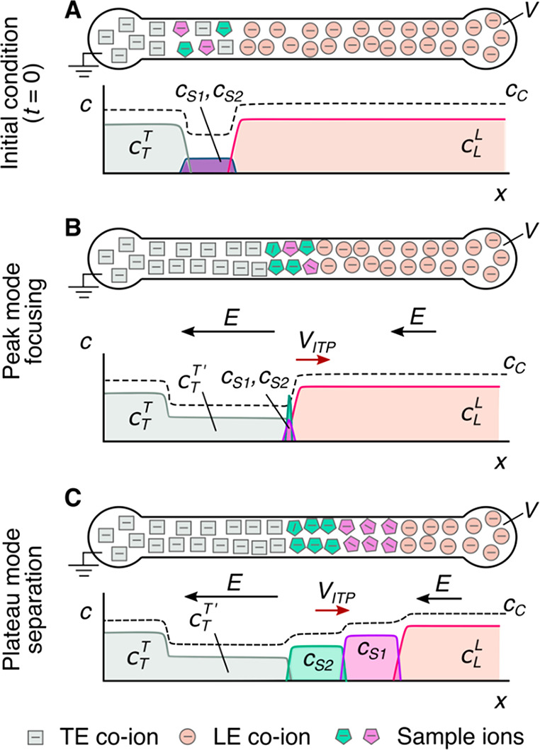
Schematic of the finite sample injection configuration for microfluidic ITP. (A) Initial placement of the LE, the TE, and the sample, common to both peak- and plateau-mode ITP. (B and C) Peak- and plateau-mode ITP focusing, respectively. Each subfigure shows the locations of ions within the channel (top) and the concentration profiles of the electrolytes (bottom) in anionic ITP. For finite injection, when the experiment is sufficiently long, all sample ions focus in ITP, leading to steady-state concentration fields of focused ions. This is unlike the case of semi-infinite injection (Figure 1), which is associated with continuous sample focusing in ITP (i.e., the focused sample amount increases with time).

A second approach for introducing a sample in ITP is called semi-infinite injection. In semi-infinite injection, the sample is initially mixed with the TE buffer (but can also be mixed with the LE or both the TE and the LE) prior to being loaded on a chip, and this mixture serves as the effective trailing electrolyte. This is depicted in Figure 1A. For the particular case when the sample is mixed with the TE buffer in the TE reservoir, the injection scheme has been called electrokinetic supercharging or electrokinetic injection.^96,97 Unlike finite injection, upon the application of electric field, analyte peaks or zones never reach a steady-state distribution. Instead, the concentrations of analytes focused in the peak mode increase directly proportionally in time (until the plateau mode is reached). After the plateau mode is achieved, the length of zones continuously increases linearly in time. This continuous accumulation can be used to improve the detection sensitivity for both peak and plateau modes. However, in semi-infinite injection, sample ions from the TE reservoir are typically never fully processed by the ITP process. A larger portion of the analytes in the TE reservoir can be processed by decreasing the conductivity (equivalently, the ionic strength) of the TE in the reservoir to achieve higher local electric fields.^39,98 A key advantage of the semi-infinite injection approach is that it is easy to implement. It is compatible with a simple straight channel geometry (i.e., no branched channels or other complex designs), and one can use a simple pipet to set up the initial TE–LE interface (at the interface between the reservoir and a channel). A drawback of the semi-infinite injection scheme is that variability in sample conductivities (as is typical of several biological samples) can affect the rate of focusing and the quantification of the amount of target analytes. This is because the rate of accumulation depends on the (possibly unknown) ratio of the sample concentration to the TE ion concentration. Hence, semi-infinite injection is most easily applied if the raw sample can be substantially diluted by the TE mixture. As an example, for the anionic ITP of physiological samples with semi-infinite injection, background sodium and chloride ions from the raw sample (which are typically present in high concentrations) can significantly modify TE buffer properties if the sample is not diluted sufficiently.

Lastly, we note that electrode’s shape and configuration determine electric field lines within the reservoir and consequently affect focusing dynamics and the amount of sample focused in ITP. For example, Rosenfeld and Bercovici⁹⁹ demonstrated that encircling half the circumference of the reservoir with a C-shaped electrode resulted in nearly twice the amount of sample being focused in ITP compared to a straight electrode. Refer to refs (100−102) for further discussions around the importance of the electrode configuration for efficient sample injection in ITP.

2.7.3. Peak- versus Plateau-Mode ITP

Peak-mode ITP is characterized by relatively low initial sample concentrations (relative to the LE and TE concentrations) and brief focusing times. Peak-mode (which has been referred to as spike mode) ITP between and the LE and the TE results from a transient process wherein ions continuously focus into approximately overlapping peaks whose concentrations are still much lower than those of the neighboring leading and trailing ions. This is shown schematically in Figures 1B and 3B; the concentration of peak-mode ions is exaggerated for clarity. If the applied current is constant (in time), the peak (and leading and trailing ions) will all travel at an equal and constant velocity, V_ITP. Often, the focused ions are several orders of magnitude lower in concentration than ions from the neighboring zone and contribute negligibly to the local current. Ions in the peak mode are therefore typically only detected directly, as in the case of fluorescent sample ions.³⁴

If sample ions are present at higher concentrations or given sufficient focusing time (assuming the sample ions are sufficiently soluble in the solvent), peak-mode ITP eventually transitions into a state where sample species contribute significantly to the local conductivity and therefore the local electric field. Such sample species begin to displace neighboring ions and segregate themselves into contiguous adjoining “plateau” regions or zones of locally uniform concentrations, as shown in Figures 1C and 3C. We refer to the latter configuration as plateau-mode ITP. When the sample is injected in a finite zone between the LE and TE zones (e.g., finite injection), species in the plateau mode reach a maximum concentration established by the properties of the LE zone. As we shall discuss, this is due to constraints imposed by the system’s regulating functions (cf. sections 3 and 4). If the applied current is constant, the plateaus (and leading and trailing ions) travel at an equal constant velocity, V_ITP. For fully ionized co-ionic species, the zone order in the plateau mode typically follows the decreasing order of the effective mobility (and exactly the decreasing order of the mobility in the case of fully ionized co-ionic species). Additionally, the widths of interfaces between adjoining plateaus are usually small relative to lengths of the plateaus. This condition of a relatively large plateau-to-interface width ratio can be used to distinguish and identify one ion from the next in the train of plateaus using a variety of detection techniques, such as electrical conductivity,¹⁰⁴ fluorescence intensity,^105,106 UV absorption,¹⁰⁷ and temperature.^1,108 The plateau mode also lends itself to the indirect detection of sample species, for example, using nonfocusing directly detectable tracers such as labeled counterions, and overspeeder or underspeeder co-ions.³³ Lastly, in addition to the plateau-forming sample ions, there may be other sample ions with significantly lower concentrations. In that case, the trace sample ions focus in the peak mode amid other plateau zones (i.e., mixed peak and plateau mode) at a location(s) that depend on the trace ion mobility value(s).

Peak-mode and plateau-mode ITP are both useful in a variety of settings (see detailed discussion in sections 3–7 and 11). Briefly, peak-mode ITP provides highly effective method for preconcentration and simultaneous mixing.^30,109−111 Peak-mode ITP can also be used to control and accelerate chemical reactions of species.^39,112 Plateau-mode ITP allows for the preconcentration, separation (including identification), and segregation of multiple sample ions.^33,104−107

3. ITP Using Strong Electrolytes

In this section, we review the theory associated with strong electrolyte ITP and provide illustrations and important limitations of this approach. We derive the so-called ITP condition using a control volume approach and then estimate the ITP interface width. We then consider a simple strong electrolyte system consisting of three ions in total and use it to illustrate the plateau-mode ITP of strong electrolytes. Next, we derive the so-called Kohlrausch regulating function from first-principles and use it to provide analytical expressions for the “adjusted” ion concentrations in plateau-mode ITP. We conclude this section by mentioning a few demonstrations and validation studies that involve the ITP of strong electrolytes. We stress that although the strong electrolyte theory is not very practical for modern microfluidic applications, which largely use weak electrolytes (including pH buffers), strong electrolyte ITP is an excellent starting point to introduce researchers to the theory and practice of ITP processes. Strong electrolyte conservation analyses are often also more intuitive for researchers with experience in classic binary electrolyte electrokinetics.^67,72

3.1. Single-Interface ITP and the ITP Condition

In this section, we use an analysis of the simplest possible form of ITP to show the connection between the net neutrality approximation and the so-called ITP condition. The simplest ITP system consists of three fully dissociated strong electrolyte species, namely two co-ions and a counterion (and no sample ion). The situation was described qualitatively in sections 2.3 and 2.7. We will consider the case of anionic ITP, where the leading (L) and trailing (T) ions are anions and the common counterion (C) is a cation. The LE and TE contain anions of high- and low-magnitude (negative) mobility, respectively, and the electric field is applied from the LE to the TE. This arrangement leads to a self-sharpening interface, with the TE and LE zones electromigrating with equal velocities V_ITP. This result of co-ions that have differing mobilities but travel at the same velocity is known as the ITP condition.

Next, we derive an expression for V_ITP in terms of the physicochemical properties of the LE, the TE, and the electric field. The relations obtained here apply to the case of cationic ITP, with minor modifications. We will first develop relations relating the jump conditions across a sharp ITP interface (e.g., the electric fields and ion concentrations) as a function of the ITP interface velocity. For simplicity, we will consider strong electrolytes (cf. eq 6). Unlike classic ITP texts,^1,2 we will formulate these jump conditions using an approach similar to the formulation of the Rankine–Hugoniot jump conditions for supersonic shock waves in compressible fluid mechanics.^113−116 In ITP, we deal with ion concentration shock waves between co-ions of various mobilities and concentrations. In general, these waves may have velocities that vary over time and space (e.g., for constant-voltage sources). We here follow an approach similar to that of LeVeque,¹¹⁶ where we consider a finite distance Δx in a stationary reference frame over which the wave propagates over a finite time Δt. The distance Δx is taken to be significantly larger than the instantaneous ITP interface shock width but sufficiently small (e.g., compared to the total length of propagation) such that the shock velocity is approximately constant. We consider then an integral formulation of the one-dimensional species conservation equation (eq 6) and integrate over distance Δx and time Δt as follows:

32

where x₀ and t₀ are, respectively, the initial position where and time at which the ITP interface enters the stationary region of width Δx. Over most of the time the thin shock traverses the distance region Δx, the diffusive fluxes at the boundaries of the region are within locally uniform concentrations, so we can well approximate these integrals as

33

The first term on the left side of this equation describes the change in the concentration of species i (from just ahead of the shock in the leading zone to just behind the shock in the trailing zone) in the Eulerian reference frame. The second term describes the change in the fluxes of electromigration species on either side of the wave. Using the approach of LeVeque,¹¹⁶ the result of the integrations can be approximated as

34

Here, c_i^L and c_i are the concentrations of species i in the leading and trailing zones, respectively; μ_i^L and μ_i are the electrophoretic mobilities of species i in the leading and trailing zones, respectively; σ^L and σ^T are the local conductivities of the leading and trailing zones, respectively; Δx/Δt is the velocity of the interface; and j is the applied current density. Note j/σ^k is merely the local electric field in region k. Dividing both sides by Δt and taking the differential limit, we obtain

35

where V_ITP is the wave speed of the ITP interface. The equation becomes exact for shock waves with uniform and constant wave speeds (as in many constant-current ITP experiments). Note that the ionic current density, j, is the same on both sides of the shock wave. Further, we can obtain the relation between the ITP wave velocity and mobilities of the co-ions by evaluating eq 35 independently for the leading and trailing co-ions. Thus, we have

36

That is, the leading and trailing co-ions travel at the same velocity equal to V_ITP. This follows from the conservation of current, i.e., j = σ^LE^L = σ^TE^T (cf. section 2.3). Note that electromigration velocities of the LE and TE co-ions are μ_L^LE^L and μ_TE^T, respectively. This result (eq 36) has historically been called the ITP condition.^117−120 Basically, the ITP condition states that the LE co-ion will electromigrate in the same direction and at the same velocity as the TE co-ion. Any trailing plateau co-ion will also travel at this velocity. Hence, this jump condition in eq 35 can be interpreted as the description of the wave velocity required so that leading ions do not “run away” from the trailing ions and leave behind counterions, which would otherwise violate net neutrality. Researchers new to ITP may find this result counterintuitive, as it describes a condition where ions of like charge but different mobilities travel through the system with the precise same velocity. We next provide a qualitative explanation for this result.

The result that even ions of even widely different mobilities can travel in the same direction at the same velocity is in fact a requirement of the conservation of current and the net-neutrality approximation. Consider that this equal velocity condition is consistent with precluding the possibility of a gap forming between LE and TE co-ions. That is, the demands of net neutrality preclude LE co-ions from speeding away from the TE co-ions. The gap would constitute a region of locally unbalanced counterions. As described in section 2.3, the typical ion densities and electric field magnitudes in ITP preclude the possibility of such grossly unbalanced charge regions.

How then do the electric fields in the TE and LE, respectively, increase and decrease to achieve this equal velocity condition? We discussed the mechanism in section 2.3. For a very short time (on the order of the charge relaxation time scale⁷⁰), the LE ions move slightly away from TE ions, forming a diffuse region that contains a tiny amount of unbalanced charge. The sign of this net charge (negative for anionic ITP) is such that it will raise the field magnitude in the TE zone while decreasing it in the LE. This tiny but important imbalance in charge builds quickly and self-limits as soon as the TE and LE co-ion velocities are equal. The latter condition ensures the conservation of current in the system, i.e., j = σ^LE^L = σ^TE^T. The result is a region of relatively high field in the TE and a region of relatively low field in the LE. The two regions are interfaced by an electric field gradient. Away from the interface, diffusive current is negligible, and we can assume that the conductivity is inversely proportional to the local field (cf. section 2.3).

As we shall see below, the established electric field gradient tends to self-sharpen and preserve a sharp interface between the ions of high and low mobility. The latter self-steeping conditions can be described qualitatively as follows. Consider a TE co-ion that diffuses out of the LE–TE interface into the LE zone. Such an ion experiences the relatively low electric field of the LE but it is “outraced” by its neighboring LE ions, and so it falls back to the interface. Similarly, an LE co-ion that diffuses into the TE zone experiences a higher local electric field, which tends to drive it back to the LE–TE interface. Even as the electric field gradient sharpens the interface, diffusion tends to try to broaden it, so the width of the interface is determined by a balance between these effects (see section 3).^79,98

We next present a more detailed derivation of the current densities, the electric fields, and the ITP velocity in terms of the specific ion valences and mobilities in the system. To this end, we will assume that hydronium H⁺ and hydroxyl OH^– ions do not contribute significantly to the current (see the safe pH approximation; cf. section 2.6). Thus, the current density from from eq 7 is expressed in terms of the mobilities and concentrations of the LE and TE co-ions and the counterion as

37

where F is again Faraday constant and E^L and E^T are the local electric fields of the leading and trailing zones, respectively. We note that eq 37 is valid for both weak and strong electrolytes. For strong electrolytes, we can avoid the subscript (location) values in valences and mobilities; for weak electrolytes, the mobilities are effective, local mobilities. For example, the term z_C^Lc_Cμ_C^L ensures the correct current contribution of the partially ionized counterion from the multiplication of the valence, the effective mobility, and the total ion concentration in the LE region.

Combining eqs 36 and 37, we get

38

where V_L^L and V_T are the velocities of the leading and trailing ions in the leading and trailing zones, respectively. Lastly, the position of the ITP interface x(t) and the voltage difference ΔV across the microchannel can be related as

39

where L is the length of the microchannel. This equation is valid for uniform cross-section channels and for either constant-current or constant-voltage operation. Moreover, the resistance in the channel increases with time as the TE replaces the LE zone. For constant-current operation, the ITP velocity is constant and uniform, and the voltage (and resistance) increases linearly with time. For constant-voltage operation, the current and the ITP velocity decrease over time in accordance with the increase in the resistance in the channel. Refer to Bahga et al.¹²¹ for a detailed derivation of the ITP velocity for the case of constant-voltage operation.

3.2. The Width of the Interface between Two ITP Plateau Zones

For a constant applied current, the ITP interface achieves a steady-state width independent of the initial conditions. This results from a self-focusing of ion concentration gradients, which is driven by nonuniform electromigration and limited by molecular diffusion. We here first present simple scaling arguments for the ITP interface width and then derive the analytical solution based on the classic work of MacInnes and Longsworth.¹²² We focus our discussion on the example of the interface between a TE and an LE zone, but the current discussion applies to the interface between any two adjoining ITP plateau zones.

We begin with an instructive scaling argument for the interface that provides insight into the self-focusing nature of ITP. The electromigration velocity magnitude of a TE ion in the LE region of the interface (or an LE ion in the TE region) can be expressed as the quantity (|μ_L – μ_T |)E, where E is some characteristic local electric field in the interface region (e.g., the average of the LE and TE electric fields). A characteristic velocity due to diffusion for the same ion scales as D/δ, where D is the diffusivity of the ion and δ is the ITP interface width. At the ITP interface, we then balance the fluxes associated with diffusion and (nonuniform) electromigration to obtain a scaling for δ as

40

This scaling suggests that the ITP interface width is inversely proportional to both the electric field and the mobility difference between the LE and TE ions and directly proportional to the diffusivity of the species.

An exact solution for the interface width between two plateau zones, δ, was first given by MacInnes and Longsworth¹²² in 1932. First, the strong electrolyte species conservation equation (eq 6) for the LE and TE co-ions in the frame of the moving ITP interface (i.e., after a Galilean transformation is performed¹²³) at the steady state can be expressed as

41

42

where ξ = x – V_ITPt is the moving coordinate of the interface and V_ITP is the ITP velocity. We next invoke the Nernst–Einstein relation between diffusivity and ion mobility (see ref (68)), written as D_i = RTμ_i/z_iF. Here, R is the universal gas constant and T is the absolute temperature. Combining these two equations to eliminate E explicitly, we derive

43

Integrating with respect to ξ and defining ξ as the location in the interface where c_L = c_T, we obtain the following for the case of z_L = z_T = −1:

44

where δ is the characteristic length scale for the ITP interface width given by

45

where we have substituted V_ITP with μ^LE^L (see eq 36).

Equation 45 shows that δ scales proportionately with the diffusivity (via the absolute value of the characteristic mobility of the Nernst–Einstein ion) and inversely with the applied current density (or equivalently, the electric field). Such proportionality is experimentally observable up to some maximum applied electric field, beyond which electrokinetic instabilities can disrupt a stable ITP interface.^98,124 It is also very useful for obtaining an intuition for the ideal conditions of (one-dimensional) ITP, wherein the interface width is limited strictly the by the competing effects of nonuniform electromigration and diffusion. However, in practice, sufficiently high currents can lead to electrohydrodynamic instabilities that limit the minimum ITP interface width (as will be discussed in section 8). Further, note that the expression for δ in eq 45 was derived exclusively for strong electrolytes in ITP; this relation does not hold exactly for weakly ionized species. Nevertheless, the length scale δ (i.e., the LE-to-TE interface width) is a useful estimate of the order of magnitude of the length scale relevant for ITP applications involving peak-mode ITP. In peak-mode ITP, the focused peak-mode minimum achievable width of the sample is governed by the finite length scale δ. Hence, this interface width affects the degree to which the sample can be preconcentrated and the reaction can be accelerated (cf. sections 5 and 7), including applications involving weak electrolytes. For typical ITP experiments in 10–100 μm channels with (typical) applied field magnitudes on the order of 20 kV m^–1, the interface width is on the order of 10 μm.⁹⁸

3.3. Condition for the Focusing of a Strong Analyte

For strong electrolyte ITP, the condition that results in an analyte ion (with a fully dissociated mobility equal to μ_s) focusing between the LE and TE zones is simply^1,125

46

where the fully dissociated mobilities of the TE and LE co-ions are, respectively, equal to μ_T and μ_L. We use absolute values in eq 46 to account for both anionic and cationic ITP.

3.4. Closed-Form Calculation for the Plateau-Mode ITP of Strong Electrolytes

The electromigration of multiple analyte species in and out of zones may at first be counterintuitive. Consider again Figure 1, which shows a simple single-interface anionic ITP system that includes an LE and a TE zone. We assume that all ion motion is due to electromigration alone (i.e., no bulk flow). The LE ions move to the right and are replaced by the influx of TE ions. Interestingly, ion displacement dynamics in this system are such that the concentration of the TE ions replacing the LE ions is completely independent of the initial TE ion concentration. Instead, the concentration at which TE ions enter the region formerly occupied by the LE is determined by the properties of the LE and the mobility of the TE ion. Hence, we find a situation where the local concentration of TE ions (in the former LE region) is independent of the initial concentration of that ion.

To further describe this effect, it is useful to define two TE-related concentrations: the initial concentration of the trailing ion (e.g., in the reservoir well, c_T^T) and the concentration of this ion after it enters the region T′ formerly occupied by the leading electrolyte, c_T. We refer to the latter as adjusted TE (ATE) concentration. As depicted in Figures 1 and 3, the interface between the TE reservoir and the ATE zone, c_T^T (and c_T), is stationary, while the interface between the ATE and LE, c_T^T′ (and c_L), moves at V_ITP. We next derive the concentration c_T^T′ of the trailing co-ion in the ATE region using the concepts of current conservation, charge neutrality, and the ITP condition.

Assuming a safe pH (cf. section 2.6), current conservation yields

47

We do not use superscripts for mobility or valence in eq 47, since these quantities are constant and uniform for fully ionized species. (e.g., μ_C^L = μ_C = μ_C). We also assume a moderate pH (cf. section 2.6) such that charge neutrality in the LE and ATE regions yields

48

Lastly, the ITP condition yields

49

Combining eqs 47–49, we obtain

50

Equation 50 can be interpreted as the condition that the sum Σz_ic_i/μ_i) in the relevant zone (here the region of ATE) is preserved whether it is occupied by LE or ATE ions. We shall show in the next section that the preservation of this sum, called the Kohlrausch regulating function, must hold in all channel locations for an arbitrary number and an initial distribution of strongly ionized species. From eqs 50 and 48, we obtain the concentration of the trailing ion in the ATE zone for the univalent case of z_L = z_T = −z_C = −1 as follows:

51

Notice that the concentration of the TE ion in the ATE zone, c_T^T′, is independent of the initial TE concentration, c_T, and solely dependent on both the LE co-ion concentration and the mobilities of the LE and TE ions. The concentration of the counterion in the ATE can simply be obtained from charge neutrality c_C^T′ = −(z_T/z_C) c_T = c_T^T′), where the second equality is for monovalent ions, z_T = −z_C = −1. We will consider multivalent species in the next section.

3.5. Kohlrausch Regulating Function and the Concept of Adjusted Concentrations

We can generalize plateau-mode ITP for an arbitrary number of strong electrolytes and also derive the “adjusted” concentration of a focused ion in any arbitrary plateau zone between the LE and the TE using the Kohlrausch regulating function (KRF). The KRF is a conservation principle that is applicable to the arbitrary electrophoresis of mixtures of fully ionized species. It was originally derived by Kohlrausch in 1897, who called it the “Beharrliche funktion”.¹²⁶ Below, we present our derivation of the KRF, summarize its assumptions, and apply it to a generic case of plateau-mode ITP of strong electrolytes.

We begin with the species conservation equation (eq 6) for the case of no bulk flow and a strong electrolyte i. We multiply and divide eq 6 by the valence and (fully ionized) mobility of the species to obtain

52

Summing eq 52 across all the species i = 1 to N, we have

53

Next, we assume moderate pH, use the charge neutrality approximation for the entire system, i.e., ∑_i = 1^Nz_ic_i = 0, and neglect diffusive terms (since ∂c_i/∂x vanishes away from sharp ITP interfaces). Thus, eq 53 reduces to

54

where w(x,t) is now only a function of x, i.e., w = w(x). The function w(x) is defined as the KRF and is given by

55

We see from eq 55 that the KRF is simply the summation of the ratios w_i = z_ic_i/μ_i over all ionic species at each point in space. Since the partial derivative of w with time is zero, the regulating function establishes a constraint on ion concentrations in space. This constraint is established by the initial condition. In practice, this initial condition is determined by, for example, the result of some preliminary process where pressure-driven flow was used to inject various electrolyte mixtures into various contiguous zones along some channel. The analysis shows that the value of the KRF along the channel is thereafter invariant with time (but can vary with x, as determined by the initial condition). In ITP, since i can refer to any ion in the system, the KRF relation applies to (i.e., governs) all zones, including any trailing zones. It is important to note that eq 54 is not accurate at the interface between zones where diffusion effects due to strong concentration gradients are important.^127,128 Consistent with this, and importantly, the KRF cannot be used to compute the concentrations of ions in the peak mode. Peak-mode ions do not contribute significantly to local net neutrality (since these ions have concentrations that are several orders of magnitude lower than those of the background LE and TE ions) and exist solely within a region of strong diffusive gradients. For example, consider a trace sample ion initially at a concentration 100 pM that is focused in peak-mode by 1000-fold to a new maximum peak concentration of 100 nM using a 100 mM LE zone. For such a species, the concentration predicted by the KRF (and established by the LE zone) would be ∼10–100 mM, which is about 5–6 orders of magnitude higher than the actual peak concentration. The latter discrepancy arises from the incorrect application of the KRF to predict peak-mode ion concentrations.

The KRF can be mathematically interpreted as the Riemann invariant that corresponds to the zeroth eigenvalue of the governing hyperbolic equations for species transport.^114,115 The levels of concentration of ions that replace an original mixture of ions via electromigration are constrained by the concentrations and mobilities of all ions that initially occupied that space. For fully ionized species, the constraint of the KRF requires that the quantity Σ_iz_ic_i/μ_i of “newcomer” ions matches the scalar value of Σ_iz_ic_i/μ_i as governed by the “former occupant” ions.

An intuition for the KRF is as follows. For each region in space, ions are not “allowed” to enter with arbitrary concentrations. Instead, ions enter each region with species-specific fluxes and species-specific contributions to the current density. These species-specific flux quantities are determined by a (global) electric field and the respective valence and mobility of each ion. The KRF reflects the precise balance through which the fluxes and current contributions of these species satisfy both species conservation and the local net neutrality of charge at all times.

To show its utility, we now apply the KRF to obtain the concentrations of plateaus in ITP. For simplicity, we consider a single counterion C common to all plateau zones. We consider the plateau region of a sample ion, X, which moves into a region previously occupied by the LE zone. Note that X represents some co-ion that can be either any one of the (several) sample ion zones or the trailing ion T in the adjusted TE zone (see Figure 4). As an illustration, consider the location marked by the dashed vertical line at x = x₀ in Figure 4, where X = S₁. The initial condition at t = 0 is set by the ions that originally occupied that region. The initial KRF value at x₀ is thus

56

Here, we used charge neutrality in the second equality. At some later time t₁, consider that the location at x = x₀ is occupied by the “newcomer” ion X as well as the original (same) counterion. The KRF at this location at time t₁ is

57

Equating the KRF at times t = 0 and t₁, we obtain

58

Equation 58 can be rearranged to obtain the concentration of the arbitrary sample X at x = x₀ as

59

Hence, c_L^L determines c_X by establishing a local invariant KRF value. Note also that eq 51 is a special case of eq 59 where X represents the TE ion in the ATE zone. Typical values for a fairly wide range of mobilities yield c_X^X values of roughly a factor of 0.5–0.9 the value of c_L. Equation 59 shows how plateau concentrations are proportional to leading ion concentrations and have values roughly equivalent to (and typically a bit lower than) c_L^L. This also shows that high initial-to-final sample concentration ratios can be achieved using a high c_L and low concentration in the sample reservoir, c_X^W (here W is used to denote “well” value, i.e., the concentration in the sample reservoir). As before, the concentration of the counterion in zone X can simply be obtained from the charge neutrality as

60

Note that z_L and z_C have opposite signs, so the second equality in eq 60 is overall a positive quantity. Later in sections 6 and 10 we will extend the current analysis to include sample accumulation rates in plateau zones and the sensitivity and resolution associated with detection of the separated zones, respectively.

Figure 4.

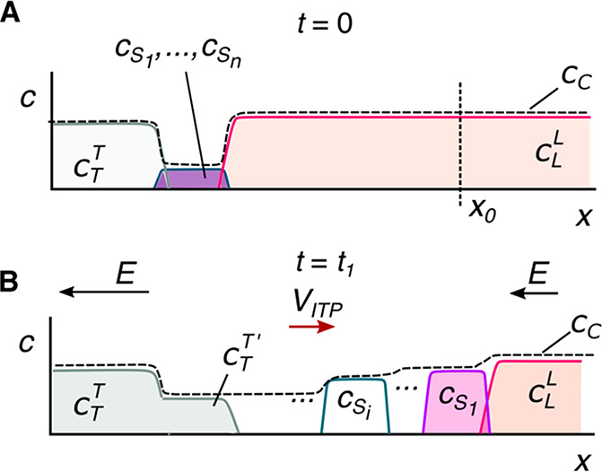
Concentration profiles for strong electrolytes in plateau-mode ITP. (A) Finite injection sample loading configuration. The sample contains a mixture of ions S₁, ..., S_n, which focus in ITP. (B) Sample ions are focused and stack in the descending order of (magnitude of) mobility values between the LE and the TE. The vertical dashed line in panel A indicates an example location along the channel where we chose to illustrate the application of the Kohlrausch regulating function, as shown in section 3.5. The S₁ ion and counterion at x = x₀ must meet the KRF set by the LE zone that originally occupied this region.

3.6. Illustrations and Limitations of the Strong Electrolyte ITP Theory

The earliest demonstration of the ITP of strong electrolytes was in 1932 by Kendall and Crittenden,¹² who reported the separation of rare earth metals and simple acids using ITP. They called their process the “ion migration method”. Importantly, this study qualitatively described that the zone concentrations automatically “adjusted” themselves to ratios governed by the KRF. Much later in 1980, the study of Hjertén et al.¹²⁹ was the first to quantitatively and experimentally validate the KRF conservation principle in ITP. The authors validated the KRF in both cationic (K⁺, Co²⁺, and Cu²⁺) and anionic (Cl^– and 5-sulphosalicylic acid) ITP systems involving strong electrolytes. To obtain accurate data for validation, Hjertén et al.¹²⁹ carefully performed ITP experiments in free solution, suppressed electro-osmotic flow (EOF), used a photoelectric scanner to determine attainment of steady state conditions, and collected ITP-separated zone fractions for downstream measurements of conductivity and concentrations.

ITP applications involving strong electrolytes were significantly developed and widely employed throughout the 1950s and 1980s. We do not review these in detail but refer the reader to a few studies involving the theory and applications of strong electrolyte ITP, including the separation of trace elements, heavy metals, and isotopes, among many others.^{13,86,134−137,122,127−133} Typically, ITP systems involving only strong electrolytes are not buffered, and such systems can exhibit highly variable (and difficult to control) pH values across zones.¹³⁸ For this reason, modern microfluidic ITP applied to biological systems seldom involves strong electrolytes exclusively. Extreme pH values can result in additional zones and dispersed interfaces (e.g., due to EOF^61,139) and lead to complex zone structures.^136,140 We refer to the studies of Gas et al.¹⁴¹ and Ermakov et al.¹⁴⁰ for a detailed theoretical discussion and associated experimental validation of ITP at extreme pH conditions.

As mentioned earlier, we here cover strong electrolyte ITP as a starting point of instruction. This theory is also useful for providing closed-form analytical solutions, which can be used to benchmark new computational approaches and simulation results.^{78,127,142−144} For an example illustration and benchmark of a strong electrolyte ITP simulation, see Figure 5.¹³⁶Figure 5 shows simulation results of an ITP system involving exclusively strong acids and bases. The study validated steady-state predicted concentrations with numerical results shown in Figure 5. Figure 5 also shows the KRF’s invariance in time at every location between the initial and final states. Notably, Figure 5 also highlights a small inverted peak (indicated by an arrow in Figure 5) in the computed KRF value at the zone boundary. Note this is a small region of high diffusive gradients in the initial condition.

Figure 5.

Simulated cationic ITP run for a LE mixture consisting of 10 mM potassium ions and 5 mM sulfate ions and for a TE mixture consisting of 10 mM sodium ions and 5 mM sulfate ions. (A and C) Concentration fields at t = 0 and t = 1.1 s, respectively. (B and D) Value of the Kohlrausch regulating function (KRF) versus the channel location x at t = 0 and t = 1.1 s, respectively. Simulations were performed using Simul software¹⁴⁴ with the following parameters: a capillary length of 3 mm, a driving voltage of 50 V, and an x-coordinate mesh consisting of 1000 nodes. The figure was reproduced with permission from ref (136). Copyright 2007 John Wiley and Sons.

4. ITP Using Weak Electrolytes

In this section, we review the theory for ITP processes involving weak electrolytes. Weak electrolytes are important, as they enable the use of pH buffers crucial to systems that process or analyze biological species. Weak electrolytes are also used extensively for several applications, including basic biochemistry, cell biology, food and plant sciences, and biological assays at the molecular, cellular, or tissue level.^31,145−153 pH buffering is also important for well-controlled processes and assays involving chemical assays and synthesis.^31,77,154

An important complexity of weak electrolytes is that, unlike eq 6 above, conservation equations necessarily involve multispecies source terms, and chemical conditions have a strong impact on the spatiotemporal development of the ionization state (including effective species mobility). To illustrate this complexity (and the failure of the Kohlrausch regulating function), consider a special case of weak electrolyte transport (eq 3) for the following special case. We neglect diffusive fluxes, multiply by the valence, divide by the mobility, and sum over all species families and ionization states to derive

61

Applying the net-neutrality approximation, i.e., Σ_i,zzc_i,z ≈ 0, we derive the following expression for the temporal change of a Kohlrausch-like variable, w:

62

The result shows that we must express w as a function of time and space. Note that the production term results in the spatiotemporal development of the variable w, so we are unable to derive a “simple” KRF for weak electrolytes. This is an important point, as the KRF is very often improperly applied to analyze ITP systems involving a weak electrolyte^{14,85,155−160} and such analyses can result in grossly incorrect predictions of ITP dynamics and species concentrations.

We are unaware of regulation functions applicable to generalized weak electrolyte systems that involve either multiple species where one or more is a multivalent species or extreme pH values outside the aforementioned “safe” and “moderate” ranges. Fortunately, there are known and convenient regulation functions for weak electrolytes that are applicable to the specialized case of univalent families (chemical families with only neutral and univalent members) and for safe and moderate pH. The latter regulating functions are called the Jovin¹⁶¹ and Alberty⁴¹ functions, which we discuss in this section. In addition, we discuss conditions for the focusing of a weak analyte in ITP, derive steady-state concentrations in plateau-mode ITP using the regulating functions, and provide some results of the weak electrolyte theory.

4.1. Conditions for the Focusing of a Weak Analyte

We know of no reference that summarizes the general conditions required for the focusing of sample species in the case of weak electrolytes and for both plateau and peak-mode ITP. We here propose a set of relations for such focusing between LE and (adjusted) TE co-ions. Consider that various zones in ITP will have different pH values, and the various ion mixtures in these zones can lead to different degrees of ionization. Hence, for weak electrolytes, we have to describe conditions for focusing in terms of effective (not fully ionized) ion mobilities and the position in space. We first consider the case of an ion X focused in a plateau region X somewhere between the LE and the ATE. The propensity of the ion to electromigrate out of the ATE region and focus within zone X (and for the TE ion to fall back from zone X into the ATE region) is given by

63

Likewise, we also require such stability conditions for the interface between zone X and the LE.

64

For the case of a single ion X focused in THE peak mode and sandwiched by the ATE and THE LE, the condition for focusing can be expressed as

65

That is, for THE peak mode, no formal (plateau) zone X exists, and ion X is subject to the electric field gradients (and relative ion velocities) established by the TE and LE co-ions.

Lastly, we note that ITP should exist in all cases, hence

66

4.2. Weak Electrolyte Regulating Functions: Jovin and Alberty Regulation

As we discussed earlier, the KRF conservation principle is not applicable for weak electrolytes. We can, however, define two regulating functions applicable to weak electrolyte systems for the special case of, at most, singly ionized species and systems that obey the safe and moderate pH conditions. These two very useful and fundamental functions are the Jovin and Alberty functions, which are described in the following two sections. To our knowledge, the current review is the first presentation of the derivation of both of these functions starting from the one-dimensional unsteady conservation equations. The authors find this remarkable given that the Alberty and Jovin functions are fundamental to the analysis of ITP, a useful method that has been in use for nearly a century.

4.2.1. Jovin Function

The Jovin function imposes fundamental restrictions on the singly ionized ion concentrations achievable at any location within a multispecies electrokinetic process. It is a very useful quantity in the derivation of closed-form relations and analyses of ITP processes. Assuming negligible effects from diffusive fluxes (i.e., negligibly influenced by sharp interfaces), the weak electrolyte species conservation equation (eq 3) reduces to

67

Summing this equation over all subspecies z of the species family i and recognizing that proton donation or acceptance results in no net generation of species family i (i.e., Σ_zR_i,z = 0), we have

68

We next restrict ourselves to the simple case of a univalent weak electrolyte family (comprised of only a neutral state and a single charge state of charge 1 or −1), eq 68 simplifies to

69

where z_i is +1 or −1. Multiplying eq 69 by z_i, summing the result over all species families, and applying the safe pH assumption (i.e., that hydronium or hydroxyl ions do not carry significant current), we have

70

Here, the last equality follows from current conservation (for a negligible diffusive current). Hence, we find the so-called Jovin’s relation, originally derived by Jovin in 1973.¹⁶¹

71

Interestingly, the left-side of this relation looks similar to the summation in charge neutrality (e.g., compare to eq 30); however, the summation of eq 71 is in fact a very different quantity, since here c_i is the total concentration (and not just the ion concentration). Here, the summation is performed over the (monovalent) species families and includes a contribution(s) from the concentration of the neutral species family member (whose z = 0) multiplied by the ionization state of that species family (z_i = 1 or −1).

The Jovin function implies that total species concentrations impose a strong regulation on the entry (exit) of all ions into (out of) any particular zone in space. Unlike charge neutrality, the Jovin function involves balances between both charged and uncharged species. For example, consider the following system that consists of just three species families. A certain zone is originally occupied by a single weak acid (comprised of members A1_–1 and A1₀) and a single weak base (comprised of C₀ and C₊₁). The Jovin function dictates that the influx of each single molecule of a new acidic species family A2 (comprised of A2_–1 and A2₀) must necessarily result in either the removal of one molecule that is a member of the co-ionic family A1 or, alternately, the addition of one molecule that is a member of the counterionic family C. Of course, the net neutrality assumption is in addition to (and separate from) the Jovin function constraint.

4.2.2. Alberty Function

The Alberty function is a second fundamental constraint on singly ionized ion concentrations. Like the Jovin function, it is very useful in the derivation of closed-form relations and analyses of ITP processes. To derive the Alberty function, we begin with eq 69 and again restrict ourselves to a single ion type per family.

72

Here, we used the relation μ_i,z_i = z_i |μ_i,zi |, since we considered a single ion per family that was univalent (i.e., z_i was restricted to values of −1, 0, or 1). Dividing eq 72 by |μ_i,zi | and summing over all species, we derive

73

where the last equality follows from the charge neutrality approximation for moderate pH. We thus obtain the so-called Alberty’s condition (originally derived by Dismukes and Alberty in 1984) as⁴¹

74

At first glance, Alberty’s relation is similar to the KRF, as it involves a summation of ratios of the concentration and the mobility across species. However, the Alberty function is in fact much different because here c_i is the total (analytical) concentration. For example, consider that ratios involved in this summation can include ratios of the total concentration of an ion family, which is primarily (and can be entirely) in an uncharged state, divided by the mobility of the (possibly locally nonexistent) charged state of that species.

Like the Jovin relation, the Alberty relation imposes a constraint that involves the concentration of both neutral and ionic species. Conceptually, the Alberty condition states that the displacement of one ion from a zone (e.g., the LE co-ion zone being replaced by the influx of a plateau zone co-ion) must be accompanied by a decreased concentration if the mobility of the new ion is lower. One important consequence of the Alberty relation is that successively trailing plateaus in ITP tend to have progressively lower concentrations (as one moves from the LE to the TE).

Together, the Jovin and Alberty functions, net neutrality, and conservation of current help us design, analyze, and build intuitions for the ITP of weak electrolytes. We will therefore invoke these relations in subsequent sections of this review.

4.3. Plateau-Mode ITP for Weak Electrolytes

As an important example of the plateau-mode ITP of weak electrolytes, here were discuss the common situation of a well-buffered anionic ITP system. Such as system can often use a weak base counterion to buffer the LE as well as every trailing plateau zone. Consider the ITP system depicted in Figure 6. Here, C is the weak base (comprised of the neutral species and the cation with z = +1), X is a weak acid analyte, and L is a leading ion. As a specific example of a leading ion in anionic ITP, we here consider chloride, Cl^– (although the discussion will apply generally to any leading ion). Note that the conjugate acid ion C⁺ implies the migration of the species family C from the LE toward the TE and hence helps establish acid–base equilibrium in all zones. To make the LE zone (and the trailing sample zones) a robust buffer (cf. section 8), a good choice for the total concentration of counterion c_C is approximately twice the concentration of HCl (equivalently Cl^–, since HCl is fully dissociated) in the LE zone. We can formulate and solve for the co-ion and counterion concentrations in all zones that trail the LE zone (including the ATE). One approach to this is to formulate current conservation, mass balances, and the ITP condition in an approach similar to what we did in section 3 for the case of strong electrolytes. However, the formulation of the problem is much more compact if we restrict our discussion to at most univalent weak electrolytes in the safe and moderate pH range and thus leverage the Jovin and Alberty functions. Interestingly, the resulting formulation will hold for both strong and weak electrolytes with the understanding that the mobilities for strong electrolytes are equal to the fully dissociated values (which are independent of the location).

Figure 6.

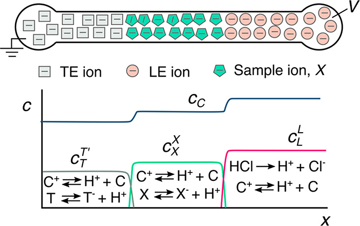
Schematic of plateau-mode anionic ITP. The top panel depicts the spatial location of leading L, trailing T, and sample X co-ions in the channel, and the bottom panel depicts the associated concentration profiles. Also shown in the bottom panel is the counterion C concentration profile and the local (rapid) acid–base chemical equilibrium reactions within each zone.

The concentration of a trailing univalent sample species X (strong or weak electrolyte) in its ITP zone can be related to the LE concentration using the Jovin and Alberty conservation laws. First, Jovin’s condition is applied to the system in Figure 6 for the spatial location currently occupied by zone X. We evaluate the Jovin summation at the initial state (when that location was occupied by the LE zone) and the current state as

75

where c_i^j denotes the total (analytical) concentration of species i in zone j. Here, subscripts i = L, X, and C refer to the leading ion, species X, and the counterion, respectively, and superscripts j = L and X are the leading and sample zones, respectively.

Next, Alberty’s condition for the leading and sample zones at the initial and final states in zone X gives

76

Here, |μ_i^j | refers to the magnitude of the fully ionized mobility associated with species family i in zone j. Combining the Jovin and Alberty relations (eqs 75 and 76), we obtain the total concentrations of species X and the counterion C in zone X as

77

and

78

Note the latter expression for c_C^X follows from eq 65 and charge neutrality. This is a closed-form solution for the total concentration of ion X in zone X. We next simplify the above expressions by neglecting the effects of ionic strength on the mobilities of the species and neglecting temperature differences between the leading and trailing zones (see refs (77), (162), and (163) for further discussion of these effects). Under these assumptions, the fully ionized mobility of the counterion (that originates in the leading zone and moves to the sample zone) remains unchanged, so |μ_C | ≈ | μ_C^L |=|μ_C |. For simplicity, we drop the superscripts on the fully ionized mobilities of X and L and assume that these values are constant (independent of zone), i.e., |μ_X |=| μ_X | and |μ_L^L|=| μ_L |. Therefore, c_X and c_C^X can be simplified as

79

and

80

Again, it is important to emphasize the mobilities here are each fully ionized mobilities (for valence magnitudes of unity), while the concentrations are total (analytical concentrations involving charged and uncharged species). Also note that, for a strong electrolyte leading ion like chloride, the analytical concentration is equal to the ionic concentration. Species family X in this equation is any species family comprising an anion that occupies a space formerly occupied by the leading ion (including any plateau sample ion or the TE ion of the ATE zone). Further note that, for the special case of strong electrolytes, we can drop all superscripts and show that, for the case of univalent species, eqs 79 and 80 are equivalent to eqs 59 and 60, respectively, described earlier.

As with strong electrolytes, a good rule of thumb for a typical weak electrolyte ITP system is that a trailing ion X achieves a total concentration of about c_X^X ≈ 0.5–0.9c_L. In other words, the total (analytical) concentration is “governed” by the LE co-ion c_L^L, while the ionic concentration of the trailing ion depends on c_L and the pH (which can depend on the relative pK_a of the trailing and counterion). Note that the adjusted TE properties can be obtained by simply replacing species X and zone X with properties of the TE co-ion T and the adjusted TE zone ATE, respectively. Finally, for a trailing ion with a pK_a significantly lower than that of the weak base, the concentration of H⁺ (equivalently, the pH) in any trailing zone can be solved in terms of the analytical concentrations. In this case, the trailing anion is approximately fully ionized, and hence we obtain a simple expression for c_H (from eq 20).

81

For such anionic ITP, the pH values of trailing zones are typically near and slightly higher than that of the leading electrolyte zone.

The pH buffering dynamics presented in this section can be summarized as follows. The typical situation is to choose a common (to both the TE and the LE) counterion with a convenient pK_a. This ion will serve as the pH buffering species, and the LE co-ion will serve as a titrant. The counterion migrates back into the TE with a concentration that is roughly twice that of the TE co-ion. In this way, the LE and TE co-ions of anionic play the role of titrant to the weak base that buffers the counterion. Again, we refer the reader to refs (76) and (77) for a good introduction or review of the electrophoresis of weak electrolytes, including pH buffers.

4.4. Illustration of Weak Electrolyte Theory and Limitations

Figure 7 shows simulation results from ref (136) for a cationic ITP process consisting of two buffer solutions comprised of 10 mM univalent strong cations Na⁺ and K⁺ and buffered by 20 mM MES, a common univalent (counterion) weak acid. The entire system is buffered around a pH of 6.1 and is within the safe and moderate pH range, so both Jovin and Alberty conservation principles are applicable. Indeed, this is seen by the values of the Jovin (W₀₀⁽²⁾) and Alberty (W₀₀) functions at the initial and final states in the plots on the right side of Figure 7 (these variables are equivalent to the small case w used in this review). Notice also that the values of MES (counterion) and Na⁺ (trailing ion) “adjust” in the adjusted TE zone based on the concentration of the LE and the pH of the zone (eqs 79 and 80). Similar to the case depicted in Figure 7, many of the species of interest for ITP, especially for biological applications, are weak electrolyte species. In section 8, we will discuss the rationale behind the need for buffering in ITP using weak acids and bases, and also provide some guidelines for the choice of buffering ions. As with strong electrolytes, the weak electrolyte theory presented above for steady-state concentration profiles of plateau zones can be used to validate the accuracy of numerical codes. We here also point the reader to refs (1) and (164−168), which contain extended lists of the pK_a values, fully ionized mobilities, possible ionization states (valence), and other physicochemical properties relevant to the ITP of both strong and weak acids and bases.

Figure 7.

Simulated cationic ITP run for a LE mixture consisting of 10 mM potassium ions and 20 mM MES and a TE mixture consisting of 10 mM sodium ions and 20 mM MES (pH 6.1). (A and C) Concentration fields at t = 0 and t = 1.1 s, respectively. (B and D) Values of the Alberty⁴¹ (W₀₀⁽¹⁾) and Jovin¹⁶¹ (W₀₀) functions versus the channel location x at t = 0 and t = 1.1 s, respectively. Simulations were performed using Simul software,¹⁴⁴ with the following parameters: a capillary length of 3 mm, a driving voltage of 50 V, and an x-coordinate mesh consisting of 1000 nodes. The figure was reproduced with permission from ref (136). Copyright 2007 John Wiley and Sons.

Though the theory presented in sections 4.1–4.3 is applicable only to univalent weak (and strong) electrolytes within the safe and moderate pH range, we note tthat his covers most practical microfluidic ITP applications. We refer to refs (78), (136), (140), and (169) for the modified conservation principles that govern acidic or alkaline (outside the safe pH range) ITP systems, including systems that contain ampholytes and significant ionic strength effects. Note that systems involving multivalent weak electrolytes often require additional conservation laws, which can in principle be formulated as solutions to an eigenvalue problem derived from the species conservation equations.¹³⁶ However, there are currently no generally applicable analytical solutions for such systems, and these solutions often do not admit any Kohlrausch-, Jovin-, or Alberty-type conservation principles. ITP systems that do not admit such conservation are also referred to as non-conservative.¹³⁶ An example of such a system is a buffer that consists of sodium (titrant) and oxalate (buffering ion) within certain ranges of concentration.¹⁷⁰

We also note that the physicochemistry of ITP summarized here is strictly only applicable for ionic strengths lower than about 20 mM. Higher ionic strengths can require additional physical considerations due to the effects of the ionic strength on the ion mobility.¹⁶⁹ Such effects primarily cause a reduction in the mobility of ions. Ionic strength also (and independently) affects pK_a values of weak electrolytes. Several models of varying degrees of complexity exist to capture such nonideal effects on ITP.^{169,171−174} In addition, effects of Joule heating or temperature differences between zones can also affect the physicochemical properties of ions and in turn affect the ionization state and effective mobility of the ions.^{162,163,175,176} Predicting ITP dynamics in such systems often requires a computational approach (see section 9). Nevertheless, the relations presented here are still very useful in the design of ITP systems, including back-of-the-envelope estimates and buffering requirements with reasonably good approximations for ionic strengths less than or about 100 mM.

5. Peak-Mode ITP Dynamics

In this section, we review simple theory and models useful in the prediction of analyte accumulation rate and the focused species shape in peak-mode ITP. Peak mode is a useful mode of ITP wherein one or more trace species are accumulated at an interface between a pair of (or multiple pairs of) plateau regions (see Figure 1).⁹⁸ Peak-mode ITP is best suited for trace (i.e., very low initial concentration) analytes and is an excellent focusing (or preconcentration) technique. Furthermore, peak mode may be necessary when one is working with a sample that has limited solubility. In its simplest form, peak mode focuses a single targeted analyte between the LE and ATE zones. If the analyte’s effective mobility is sufficiently large (small) compared to the trailing (leading) plateau, then the analyte ion tends to focus within a very narrow peak that is approximately Gaussian in shape. In peak mode, the analyte contributes insignificantly to the ionic current and so the local ionic current and electric field distribution is dominated by the effects of the two neighboring plateau zones. Peak mode is generally associated with assays wherein the analyte is directly detectable. Example applications of this include the selective focusing and direct detection of fluorescent species,^27,30,111 the extraction and purification of a target species (most notably nucleic acids but also proteins from blood, tissues, or cell lysate),^{31,32,90,110,177} and the preconcentration and cofocusing of reactants to accelerate chemical reactions (see sections 7 and 11).^39,112 Of course, the very early stages of the focusing of any ion at virtually any initial concentration (e.g., on the order of or less than the concentration of the ATE) is a peak-mode focusing. If allowed to proceed for a sufficiently long time, the focused analyte will eventually transition into a plateau and displace and separate the adjoining plateaus.

5.1. Analyte Accumulation Rate

We here present a control volume (CV) analysis useful for deriving relations for the accumulation rates of trace analytes in peak-mode ITP. For this, we choose a CV that moves with the ITP zone at V_ITP and extends from the adjusted TE region to the LE region across the interface, as depicted by the dotted lines in Figure 1B. We denote the sample (a.k.a. analyte) ion of interest using S and, for simplicity, consider a constant-current ITP operation in a channel with uniform cross-sectional area A (see Bahga et al.¹²¹ for the analytical theory applicable to ITP in channels with varying cross-sections). For simplicity, we further assume negligible pressure-driven flow and EOF (for example, see Garcia-Schwartz et al.⁶¹ for the effects of internal pressure gradients due to EOF on peak-mode ITP). For this simple peak-mode case, the species transport equation for focusing sample in the moving frame (based on eq 3) is³⁹

82

Here, the Galilean reference frame is moving at V_ITP, and x is measured along the direction of travel of the anionic ITP zone. The subscript S refers to some ionic sample species that focuses between the TE and LE zone. Here, we have introduced the primed quantities to indicate the local evaluation both in our control volume and within the adjusted TE zone. We now consider the case of the semi-infinite injection of the sample where it is homogeneously mixed with the TE buffer (including in an upstream reservoir). We then perform an integration of this equation over a CV that includes a large portion of the adjusted TE and is bound by the ITP interface. We apply the divergence theorem to the right side and derive

83

The left side of eq 83 is simply the rate of accumulation of the total moles of species N_S within the ITP peak (e.g., in units of moles per second). The right side of eq 83 involves the summation of fluxes over the control surfaces, which include the top and bottom channel walls (where the sample flux is zero) and the left (adjusted TE) and right (within the LE, just to the right of the TE-to-LE interface) faces of the CV. On the right face of the CV, the sample concentration is locally zero for our case, so the corresponding integrand is zero. On the left face of the CV (well within the adjusted TE region as per our CV definition), the sample concentration is locally uniform (i.e., no diffusive flux). Therefore, eq 83 simplifies to

84

where we have used V_ITP = μ_T^T′E_T′ and introduced the so-called separability^178,179 factor p_S,TE = (μ_S/μ_T^T′) – 1. Note that c_S is the adjusted concentration of the sample in the adjusted TE zone, which is equal to the product of the initial sample concentration in the reservoir c_S^W and the ratio of electric fields in the TE and adjusted TE zones.⁶⁴Equation 84 shows that the sample accumulation rate in ITP is proportional to the initial sample concentration in the reservoir and the mobility difference (equivalently, the separability) between the sample and TE co-ions in the adjusted TE zone. The terms on the right side of this equation are (for constant current) constant (in time), so the total amount of accumulated sample as a function of time is simply given by

85

Further, for the present case where the effects of bulk flow are negligible, we have l = V_ITPt. Here, l is the distance swept by the ITP peak along the channel in time t. Thus, the amount of accumulated sample can be expressed in terms of l as

86

where ∀ is the volume swept by the ITP zone as it migrates through the channel (a concept very useful in the more complex case of channels of varying cross-sections¹²¹). Equations 85 and 86 show that the total moles of sample that accumulate in the ITP peak increase proportionally with both time and the distance swept by the ITP peak along the channel. We note that our formulation above is valid in the limit of the negligible depletion of the trace analyte from the TE reservoir, e.g., when the reservoir-to-channel volume ratio is high such that the concentration of the sample in the TE reservoir is approximately constant. Refer to Eid and Santiago⁶⁴ for the derivation of accumulation rates in ITP in the regime of significant depletion of the sample from the reservoir. Note further that the expressions for the peak-mode accumulation rate (eqs 84–86) were obtained for the case when the sample was initially dissolved in the TE. Similar expressions can be obtained for the case when the sample is dissolved in LE by simply replacing p_S,TE and c_S^T′ in these equations with p_S,LE = 1 – (μ_S/μ_L^L) and c_S, respectively.⁶⁴

We next present below simple heuristics to approximate the effects of the bulk liquid flow velocity u_b (area-averaged velocity of bulk solvent) in the above control volume analysis. Bulk flow can be caused by pressure-driven flow, EOF, or both.⁶¹ For this discussion, we assume that the diffusion time for the species along the transverse direction of the channel (e.g., the radius in a cylindrical channel) is significantly smaller than the transport time of interest. Therefore, the local effect of the bulk flow can be described by a simple frame of reference change given by the area-averaged bulk flow velocity. Nonuniform velocities across the cross-sectional area of the channel (e.g., due to the no-slip condition) would also tend to disperse the sample, but we assume that the control volume axial dimension is longer than the dispersed length of the ITP zone. In this regime, the distance swept by the ITP peak is l = (V_ITP + u_b)t. Importantly, since bulk motion does not influence the rate of focusing (only drift velocities can focus species, not the divergence-free bulk flow), the rate of focusing dN_S/dt is the same as that in the case with no bulk flow (eq 84). However, bulk flow affects the relation between spatial location l and amount of sample accumulated as follows:

87

where we have used V_ITP = μ_T^T′E^T′. Integrating eq 87, we get

88

Note that the denominator V_ITP + u_b in eqs 87 and 88 can tend to very small values, implying a large amount of analyte for very long times. One example of this is the case of counter-flow ITP, where pressure-driven flow is used to counteract the electromigration of the ITP zone^60,62,180 (see Figure 8).

Figure 8.

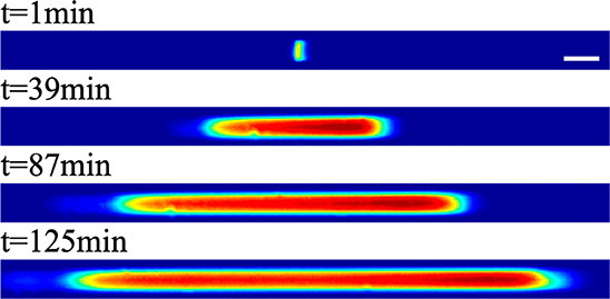
Experimental images showing the accumulation of 10 nM AF488 dye versus time in counterflow ITP. A 1 kV voltage was applied in a 5 cm capillary. The leading and trailing electrolyte are, respectively, 750 mM Tris-HCl and 10 mM Tris-HEPES. Pressure-driven flow is used to counteract ITP electromigration. The scale bar represents 50 μm. Results shown here are from an unpublished study performed by J. Sellier, F. Baldessari, A. Persat, and J.G. Santiago in the Santiago lab at Stanford University.

For the special case when bulk flow is caused by EOF alone, u_b = ⟨μ_EOFE⟩, where μ_EOF and E are the local electroosmotic mobility and the electric field, respectively, and ⟨⟩ is an axial average operator. This type of axial average is discussed by, for example, Bharadwaj and Santiago³⁵ and Garcia-Schwarz et al.⁶¹ In the case of EOF alone, ⟨μ_EOFE⟩ is a function of the location of the ITP zone. ⟨μ_EOFE⟩ tends to increase as more of the channel is occupied by the TE, since the TE typically has a lower ionic strength, a slightly higher pH (for anionic ITP), and a higher electric field (see Garcia-Schwarz et al.⁶¹).

We note that the heuristic solution presented above should be derivable from a Taylor-Aris type analysis of the transport. Such analysis would assume that the diffusion time across the cross-section of the channel is significantly smaller than the advection times of interest. The analysis would then proceed with an area-averaging of the transport equations and a Galilean transfer to a reference frame moving at velocity (V_IPT + u_b).

We note also that the analyses presented in this section assumed that the sample concentration that flowed into the control volume was constant. This assumption will not hold indefinitely, for example, for channels of significant volume relative to the channel volume. Eventually, the sample in a TE reservoir is depleted, and this depletion can result in a decaying rate of accumulation. A model for these dynamics was proposed by Rosenfeld et al.⁹⁹

Lastly, the analyses in this section were limited to a semi-infinite injection configuration. Consistent with this, we derived relations for the total amount (in moles) of accumulated species, which increased in proportion to time. However, the analysis presented here could be extended to the case of finite injection. In the case of finite injection, the accumulated sample would initially increase in proportion to time and then achieve a steady-state value as the sample was depleted from the (finite) injection zone.

5.2. Focused Analyte Shape in the Peak Mode

The shape of the focused analyte in peak-mode ITP is important to determine the relations among the maximum peak concentration, the accumulated amount, and the area under the concentration versus location curve. The peak shape can also strongly influence the sensitivity and the resolution of detection.^98,181 In the limit of low electric fields, negligible EOF, and no applied pressure-driven flow, ITP interfaces (including zone-to-zone interfaces δ and the width of the focused analyte peak δ_a in peak-mode ITP) are predicted well by a one-dimensional balance between nonuniform electromigration and axial molecular diffusion.^16,61,98 In peak-mode ITP, this regime yields an ITP focused zone that is small (δ ≈ δ_a and is on the order of the smallest channel cross section dimension), approximately Gaussian (provided the mobility of the analyte is significantly different from those of the neighboring plateau co-ions⁶¹), and inversely proportional to the current density (cf. section 3.2). In practice, this ideal one-dimensional picture of ITP is most often disrupted by one or more of the following four effects: tailing of the ITP peak due to the mobility of a focused species approaching that of a neighboring plateau (an effect different than Taylor–Aris-type dispersion^59,61), dispersion of the ITP peak due to external pressure gradients,⁶² dispersion due to residual EOF,^61,139 and electrokinetic instabilities.¹⁸²

We first discuss the first of the four aforementioned effects. For this case, the LE-to-TE interface width δ is typically smaller than the width δ_a of the analyte distribution. For simplicity, we consider the tailing behavior of a focused sample peak under ideal dispersion-free conditions. This situation represents the common case of peak-mode ITP experiments performed at moderate electric fields for which EOF is significantly suppressed and there is no external pressure-driven flow. EOF suppression can be achieved by both operating the system at sufficiently high buffer concentrations (e.g., at 50 mM and above) and introducing additives that suppress EOF, such as PEO or PEG (cf. section 8 for further discussion).^183−189

The study from Garcia-Schwarz et al.⁶¹ was the first to take into account an analyte’s physical properties to predict nonideal sample distributions (e.g., tailing and dispersion) in peak-mode ITP. They presented a one-dimensional, area-averaged, three-zone model to capture the shapes of sample zones of fully ionized species focused in peak-mode ITP (including the effects of Taylor–Aris-type dispersion due to induced secondary flows). Here, we present a simplified version of the analysis of Garcia-Schwarz et al.⁶¹ (which included Taylor–Aris analyses that described how dispersion coupled with tailing). The steady-state behavior of the analyte concentration can be obtained from eq 82 (which is applied in the frame of reference of the moving ITP interface) and is described by the following equation:

89

Equation 89 was obtained by integrating the right side of eq 82 and noting that the constant of integration was zero (obtained by evaluating it far from the ITP interface). Since the analyte concentration distribution spans the TE and LE zones, we do not use superscripts in eq 89. We will instead assume that the analyte has approximately the same mobility in the LE and the ATE. Note that in eq 89 we assume that D is simply the diffusion coefficient of the focused species, while Garcia-Schwarz et al.⁶¹ assumed an effective Taylor dispersion diffusivity to model additional effects due to EOF-driven dispersion (the analytical result shown as black dashed lines in Figure 9). In the dispersive case, dispersion effectively acts to smear and widen the already tailing dispersion-free distribution (the blue dotted curves in Figure 9 are the distributions of the diffusion-only case). Assuming fully ionized mobilities, eq 89 can be integrated directly to yield

90

where κ is a constant. This compact and intuitive result is implicit in terms of the spatial integral that involves the unknown electric field distribution but describes the shape of the sample peak.

Figure 9.

Simulation results for sample concentration fields in peak-mode ITP under conditions where the sample tails into (A) the adjusted TE region and (B) the LE region. (Top Row) Axial concentration profiles of the leading and trailing co-ions and the common counterion. (Middle Row) 2D concentration profiles of the sample obtained from the simulation. Superimposed lines are tangents to the combined electromigration and convective mass flux components. (Bottom Row) Area-averaged distributions corresponding to the dispersed and nondispersed simulations shown as red (solid) and blue (dot) curves, respectively. Analytical model predictions are as the dashed curve. A uniform EOF mobility is assumed in this figure. We refer to Garcia-Schwarz et al.⁶¹ for details about the simulation and model parameters. The figure was reproduced with permission from ref (61). Copyright 2011 Cambridge University Press.

Consider the interface region in which the analyte is focused, as shown in Figures 9A and B. The magnitude of the sample concentration in Figure 9 is typically much lower everywhere than that of the adjoining trailing and leading buffering ions (Figure 9). The tail of the sample distribution into the adjusted TE (LE) region to the left (right) is caused by a sample mobility near the trailing (leading) ion. As discussed in Garcia-Schwarz et al.,⁶¹ it is useful to conceptually divide the interface region into three zones: A, B, and C. As a heuristic approximation, regions A and C can be treated as regions of uniform electric field, and region B can be treated as one with a constant (and uniform) electric field gradient. Under this heuristic, the integral equation in eq 90 can be explicitly solved for c_S as

91

The constants a, b, c, α and σ in eq 91 can be found in the work by Garcia-Schwarz et al.⁶¹ These were obtained by ensuring that c_s values and their gradients matched at the A–B and B–C interfaces for a specified integrated amount of the focused sample. The three sections of the c_S curve are well-approximated by decaying first-order exponential tails in regions A and C and a local Gaussian “peak” region in region B. The constant σ scales the Gaussian width and is well approximated by 0.9δ, where δ is the LE-to-TE interface width. The length scales β_i describe the length of the sample peak “tail” into i = TE (T) or LE (L) zones, which can be expressed as

92

Thus, the effective width of the focused sample δ_a scales as δ + β_TE + β_LE. For the special case of analyte mobility μ̅ = 2μ_Lμ_T/(μ_L + μ_T), the concentration distribution of the focused sample is symmetric. Further, for μ_S > μ̅ and μ_S < μ̅ ,the sample will have a longer penetration length in the LE and the TE, respectively. In other words, analyte mobilities μ_S near those of the TE (LE) can cause the significant tailing of the analyte into the TE (LE). These trends predicted by the model were validated with numerical simulations and experiments by Garcia-Schwarz et al.⁶¹

Rubin et al.⁵⁹ obtained exact analytical solutions and closed-form engineering approximations for the cross-section-averaged one-dimensional analyte distribution in peak-mode ITP (diffusion-dependent with no EOF or pressure-driven flow) involving systems of weak electrolytes. Specifically, they obtained exact solutions for leading-, trailing-, and counterion concentration profiles and the electric field distribution, which were used to derive the focused sample concentration profile. The exact solution involves the hypergeometric function and is more complex to implement in practice. However, a useful engineering approximation for the sample concentration, as derived in Rubin et al.,⁵⁹ is given by

93

where b = δ/δ_a, δ^–1 = μ_T^–1 – μ_L, and δ_–1^a = μ_T – μ_A^–1 for a monovalent analyte. In this formulation, the length scales δ and δ_a are normalized by a characteristic ITP length scale RTμ_c/FV_ITP, and the mobilities are normalized by the counterion mobility. Importantly, eq 93 provides the dependence of the concentration profile on the mobility of the analyte μ_A (normalized by the counterion mobility). Equation 93 is plotted in Figure 10A for various values of the analyte mobility. Note that the maximum value of the focused sample concentration and its corresponding spatial location are strong functions of the analyte mobility (relative to that of the adjoining plateaus); see Figure 10B and C.

Figure 10.

Analytical model predictions for sample distribution in peak-mode ITP. Effect of the sample ion mobility on (A) sample concentration profiles c_a (c_S in our notation) versus x and (B) the curve relating the maximum sample concentration (and its axial position). (C) Peak concentration as a function of the sample mobility. The figure was reproduced with permission from ref (59). Copyright 2014 AIP Publishing.

Note that the models reviewed above^59,61 are experimentally validated, one-dimensional, area-averaged sample concentration distributions under ideal peak-mode ITP conditions (i.e., with no dispersion).

We next mention some work on analyses of dispersed ITP peaks. See refs (60−62) and (143) for detailed discussions around models, which include dispersion effects on sample zone dynamics due to EOF and externally applied pressure gradients (e.g., in counterflow ITP). For readers interested in the effects of dispersion due to EOF or pressure-driven flow on the LE-to-TE interface itself (independent of the focused sample dynamics), we refer to refs (8), (139), (190−192) Quantitative studies of the axial distribution ofpeak-mode ITP under dispersive conditions typically employ Taylor–Aris-type dispersion models and hence describe area-averaged one-dimensional concentration fields.^61,192

Lastly, we briefly mention some studies that attempted to consider two- or three-dimensional ITP shapes under dispersion. The source of the dispersion can be an externally applied pressure-driven flow (e.g., a pressure difference between the LE and TE reservoirs) or the dispersive velocities associated with axially nonuniform EOF (which causes internally generated and nonuniform pressure-driven flows). For example, Schönfeld et al.¹³⁹ and Garcia-Schwarz et al.⁶¹ (see Figure 9) each observed that time varying internal pressure gradients and secondary flow generated due to nonuniform electroosmotic flow in microchannels could lead to dispersed and axially distorted LE-to-TE interfaces and focused sample concentration profiles, respectively (see Figure 9). Schönfeld et al.¹³⁹ reported in qualitative observations that the LE-to-TE boundary in a microchannel ITP experiment in the presence of EOF transitioned from a ⊂-shape (concave right) to a ⊃-shape (concave left) when a larger portion of the channel was occupied by the TE. They also correctly identified that the ratio of EOF velocities in the LE and the TE determined the degree of dispersion. Later, Garcia-Schwarz et al.⁶¹ significantly expanded on the analysis of Schönfeld et al.¹³⁹ and analyzed the dynamics of a focused sample in peak-mode ITP in the presence of EOF. The latter was the first quantitative study of the radially nonuniform distribution of a focused sample in ITP. They observed focusing regimes where the sample concentrated either near the channel walls or near the channel center (sometimes achieving concentration values higher than the nondispersed case!) depending on the mobility of the analyte and the position of the ITP peak within the channel.

Three-dimensional sample concentration profiles have also been reported for peak-mode ITP in the presence of externally applied pressure gradients. For example, GanOr et al.⁶⁰ observed diffusion-dependent sample focusing regimes for counterflow ITP. They reported an approximate heuristic model for the shape of the ITP interface. Further, they identified two parameters that determined different radial sample focusing regimes, namely, the ratio of the analyte to the TE ion mobility and the ratio of the ITP velocity to the analyte diffusivity. However, note that this simple model assumes only axial velocities for electromigration and hence does not take into effect the full coupling between the electric field and the nonuniform (along cross-section) conductivity field. GanOr et al.⁶⁰ hypothesized that a sufficient condition for the radial focusing of the sample was the existence of a nonuniform axial velocity field. They also observed that focused species with nearly the same mobilities but significantly different diffusivities (e.g., small molecules versus micrometer-sized beads) could exhibit very different radially dispersed and focused concentration profiles (see Figure 11), an effect they attributed to the difference in balance between axial electromigration and axial diffusion among the focused species. The effects of pressure-driven flow on the LE-to-TE interface and sample zone dynamics in peak-mode ITP were also studied by Bhattacharyya et al.⁶² and Gopmandal and Bhattacharyya¹⁴³ using numerical simulations. To date, we know of no fully three-dimensional models of peak-mode ITP concentration fields that take into account the full coupling of electric body forces and bulk flow velocities.

Figure 11.

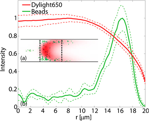
Experimental data showing effects of the diffusion-dependent radial separation of two co-focused species (DyLight650 dye and 2.8 μm magnetic beads) in counterflow ITP. The two species (green vs red in the figure) have similar mobilities but significantly different diffusivities. The figure was reproduced with permission from GanOr et al.⁶⁰ Copyright 2015 AIP Publishing.

6. Plateau-Mode ITP Theory for Separations and Sample Identification

Plateau-mode ITP is well suited for applications around the separation and identification of chemical species. Co-ionic species are typically segregated into adjoining zones between the LE and ATE zones. The order of these zones is related to the effective mobilities of the analytes (as influenced by local pH). Plateau-mode ITP is described schematically for the cases of semi-infinite and finite ITP injections in Figures 1C and 3C, respectively (cf. sections 1 and 2). The ITP focusing of low-concentration species requires that a sufficiently large volume of sample be processed to ensure the accumulation of each species into a plateau. In semi-infinite injection, plateau zones will form, but only the first zone (adjoining the LE) will be purified, as species are constantly entering the various trains of plateaus. For example, the plateau of a species adjoining the ATE zone will contain the maximum concentration of that species and also small concentrations of all other sample species that must cross that plateau as they accumulate in their respective plateaus. In finite injection, we typically eventually reach a steady state where each plateau is a locally purified. For simplicity, we will here concentrate on this finite injection case.

Plateaus that result from finite injection are regions of locally uniform concentrations that (together with the counterion) control the local conductivity. Recall from our discussion in sections 3 and 4 that plateau-zone sample concentrations are governed by the adjusted (regulated) values obtained from the Kohlrausch regulating function (cf. section 3) and the Jovin and Alberty relations (cf. section 4) for strong electrolytes and weak electrolytes, respectively. In this way, the LE zone helps determine the concentration of each plateau zone. For well-buffered ITP processes where the pH each plateau is near that of the LE, the LE zone also largely determines the effective mobility of each species and therefore the order of the zones. Note that to achieve plateau mode an ion must be soluble at its respective plateau-value concentration. As an example, consider two sample species S₁ and S₂ that focus into a sequence of plateaus, as shown in Figure 3C (cf. section 2). The plateau ions typically have concentrations that are on the same order of magnitude and very close to (but slightly lower than) the leading ion concentration. Note this is in contrast with peak-mode ITP, where the focused sample ion concentration is generally 10 orders of magnitude lower than the leading ion concentration. The conductivity (and, therefore the electric field) in each plateau is controlled by the local ion density of the sample (and the associated counterion concentration). Essentially, each sample ion “displaces” others to form its own plateau, and these sample ions segregate into plateau zones behind the leading zone in the decreasing order of the absolute values of effective mobilities. The latter sentence, of course, assumes that our system does not contain so-called “shared zones” where a single plateau is made up of two co-ionic species with approximately the same mobility.¹⁹³

The regime of plateau-mode ITP can therefore be summarized as follows: (i) high initial concentrations of species and sufficiently long focusing times, (ii) separation of species (e.g., in preparation for either direct or indirect detection), and (iii) leveraging the displacement physics of ITP (i.e., sample ions displace other ions and form locally purified zones where sample ions control current). The displacement physics of ITP can also be used to effect indirect detection methods wherein exogenous fluorescent species are introduced to detect and quantify species that are not directly detectable. The latter includes fluorescent markers, nonfocusing tracers, and spacers (cf. section 10).

In this section, we extend the theory presented previously for plateau-mode ITP in sections 3 and 4 and provide expressions for the analyte accumulation rate and the lengths of plateau zones. Much of the theory presented in this section has been covered extensively and in great detail in several references.^{1,2,85,194,195} Here, we only highlight key features of the plateau-mode ITP theory and discuss parameters useful for optimizing separation processes.

6.1. Accumulation Rate and Length of Plateau Zones

Here, we analyze the case when the sample ions are mixed with and dissolved in the TE prior to segregation in plateau-mode ITP. For simplicity, here we will assume constant mobilities for the sample and TE ions (equal to fully dissociated values, i.e., the strong electrolyte assumption). The formulation of the ITP accumulation rate for the case of a sample accumulating into a plateau directly from the trailing zone follows the same approach as that in the case of peak-mode ITP (cf. section 5). The sample accumulation rate in plateau-mode ITP is

94

Note that the expression for the accumulation rate in eq 94 is mathematically the same as that for peak-mode ITP (eq 84). The important difference in the current case is that initial sample concentrations c_S^T are typically much higher than peak-mode sample concentrations and are locally uniform within the plateau. We next present expressions for estimating the length of the plateau zone for a sample S initially loaded in the TE in plateau-mode ITP.

From the rate of accumulation into a plateau from the trailing zone given by eq 94, we can define a length for the plateau Δx_S as follows by ignoring diffusive effects and assuming univalent ions and pure zones:

95

where N(l) is the accumulated amount of sample in moles as a function of the distance l along the channel swept by the ITP zone. This expression works for both finite and semi-infinite type injection. In the former case Δx_S at first grows linearly in time and then saturates, while in the latter case Δx_S grows linearly for as long as the ITP process is run (assuming no significant depletion of sample in the reservoir). Note that we used the KRF (eq 59) to calculate the sample concentration in terms of the LE co-ion concentration. At first glance, eq 95 seems to have an inverse relation to the LE concentration. However, as we show below, N_s is also proportional LE concentration, so c_L^L will cancel out. Thus, we shall see that Δx_S is relatively insensitive to c_Lc_L^L.

Similar to peak-mode ITP (eq 86), the accumulated sample can be cast in terms of the distance l traveled by the LE zone’s trailing edge along the channel as

96

Relating the sample accumulation in the ITP zone to the entrance of channel (e.g., from the reservoir well, W) via species conservation, we have c_S^T′E^T′A = c_sE^WA. We have assumed that the well liquid presents itself slightly into the channel (so that the areas in the latter equation cancel). Thus, the accumulated sample concentration can be rewritten as

97

Here we used current continuity and the KRF. Substituting eqs 96 and 97 into eq 95, we get

98

where f is the function of the mobilities of the sample, the TE co-ion, the LE co-ion, and the counterion (f is the quantity in square brackets in eq 98) and here l is the channel length between the reservoir and the detection region. From eq 98, we see that a longer distance l and a lower TE concentration (in well) each increase the zone length Δx_S. Further, the zone length Δx_S is directly proportional to the initial (reservoir) concentration of the sample. Also important is that Δx_S is independent of the concentration of the LE.

Note that in the above derivation we assumed that the focusing species were strong electrolyte species. A similar analysis (and scaling) can be extended to weak electrolyte systems. In this context, we refer to the work of Gebauer and Boček,¹⁹⁶ who introduced the concept of zone-existence diagrams (ZEDs). ZEDs plot the zone pH versus the effective mobility using the fully ionized mobilities and dissociation constants of the species as parameters. ZEDs are useful for designing buffers and understanding the migration and zone orders of ITP separations involving weak acids and bases. This concept has been used to develop strategies to choose electrolyte systems for ITP.^197,198

7. Reactions Controlled and Accelerated by Microfluidic ITP

We here review simple models for microfluidic ITP systems where ITP is used to initiate, control, and accelerate biochemical reactions involving one or more reactants that focus in ITP.¹¹² We discuss both homogeneous and heterogeneous reaction systems. Example applications include reactions involving one or more of nucleic acids, proteins, and cells (cf. section 11.4). Most studies reviewed here use peak-mode ITP for reaction acceleration. We refer to Eid and Santiago³⁸ and Khnouf and Han⁶⁶ for recent review articles on this topic.

7.1. Theory and Models for Homogeneous Reactions

We briefly review homogeneous reactions in ITP. We define “homogenous” reactions in the context of ITP as those wherein all reacting species are solutes in solution and at least one of the reacting species focuses and preconcentrates in ITP. Consider the following standard, well-mixed, second-order bimolecular chemical reaction between species A and B that results in product AB and has forward and reverse reaction rate constants k_on and k_off, respectively:

99

For simplicity, consider the limit where one of the species, say c_A, is initially present in significant abundance relative to the other, c_B, and where the equilibrium constant is sufficiently low (K_eq ≪ c_A). The reaction in eq 99 is then well-described by pseudo-first-order kinetics. In this limit, the fraction f_std of the limiting reactant B, which has reacted to form AB, versus time t is given by

100

where c_AB is the concentration of the product, B₀ and A₀ are the initial concentrations of c_B and c_A respectively. The relation shows a pseudo-first-order reaction time scale of the form τ_standard = ln(2)/(k_onA₀) We shall see that the primary effect of ITP is to decrease the reaction time by increasing the concentration of the high-abundance species and continuously increasing the available concentration of the low-abundance species (hence increasing the production rate).

For simplicity, consider an ITP system where both reactants A and B focus and preconcentrate in ITP. Bercovici et al.³⁹ presented a system of first-order ordinary differential equations to describe such homogeneous reactions controlled and accelerated by ITP. They considered an ITP system where species A and B were initially placed in the TE and LE using semi-infinite injection, respectively (see Figure 12A). The reactants focus in peak-mode ITP and are assumed to be colocated within one-dimensional Gaussian concentration profiles c_i. A volume-averaged species concentration c̅_i within the ITP peak was obtained by averaging the concentration profiles over the ITP peak axial width δ. Bercovici et al.³⁹ derived a set of volume-averaged electromigration-reaction conservation equations for the reactants and products in ITP as

101

where Q_A and Q_B are the influx rates of reactants A and B into the ITP peak region. Q_A and Q_B are given by^39,64

102

where β is the ratio of the TE ion concentration in the adjusted TE and TE zones (the latter is assumed to be the TE reservoir), μ_i is the mobility of species i, and S is the cross-section of the channel. To simplify the analysis, Bercovici et al.³⁹ further assumed a constant ITP width δ and obtained from eqs 101 and 102 the following conservation equations for species A and B in ITP:

103

In contrast, the standard (non-ITP) well-mixed reaction obeys

104

Figure 12.

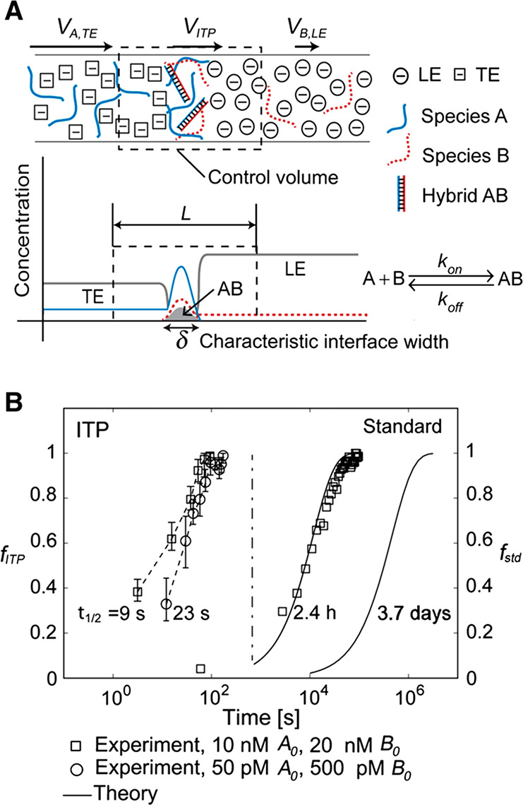
(A) Schematic of a model homogeneous reaction system in ITP consisting of two co-focused chemically reacting species in peak-mode ITP. (B) Experimental demonstration of up to 14 000-fold reaction acceleration of a DNA–DNA hybridization reaction in ITP. The latter reaction is an example of a second-order homogeneous reaction. The fraction of hybridized reactants vs time is shown for standard (well-mixed) conditions and ITP. Symbols represent experimental data, and solid lines represent model predictions. The figure was reproduced with permission from ref (39). Copyright 2012 National Academy of Sciences.

Equations 103 and 104 highlight how there is no longer a steady-state solution in ITP; instead, species continuously focus and produce a product whose growth is enhanced by the rate of accumulation and focusing.

Equations 101–103 can be simplified for the case when one of the species (say, A) is present in an excess concentration within the ITP interface and there is a sufficiently low equilibrium constant. This yields the following pseudo-first-order approximation for the concentration of product in ITP:³⁹

105

where

106

Thus, the fraction f_ITP of reactant B (low abundance) within the ITP interface that has reacted to form AB is

107

Based on eqs 105 and 107, Bercovici et al.³⁹ derived a pseudo-first-order time scale associated with ITP-mediated reactions.

108

Equations 105–108 depict two key features of ITP-accelerated reactions. First, the prefactor B_0,ITP = Q_Bt in eq 105 creates what is called a quasi-steady condition for t ≫ τ_ITP The system has no true steady state but, in this regime, tends toward a balance where the production rate is precisely limited by the accumulation rate of the low-abundance species. This results in a linear “quasi-steady” increase in the concentration of the product. Second, as shown by eqs 105 and 106, reactions in ITP have a t² in the exponent (compared to t for standard case). This t² dependence is due to the simultaneous effects of the (standard) pseudo-first-order reaction and the ITP-aided linear increase of the concentration of the abundant species (here, A) with time. The ratio of the time scales associated with reaction completion for the standard and ITP reaction conditions is then³⁹

109

From eq 109, we see that ITP significantly decreases the time for reaction to occur, especially in the challenging regime of low k_on and A₀. Bercovici et al.³⁹ reported a τ_std/τ_ITP value of ∼10 000 for A₀ = 100 pM and k_on =10³ M^–1 s^–1 under typical ITP experimental conditions. They validated the ITP reaction kinetics model with experiments using DNA hybridization reactions involving ssDNA oligos and molecular beacons (MB) and demonstrated a ∼14 000-fold acceleration of reactions that used ITP (cf. Figure 12B). Specifically, for 50 pM MB and 500 pM target ssDNA, the time scale to complete 50% of the reaction in the standard case was ∼3.7 days, while for ITP the same time scale was ∼23 s for the same initial concentration. This corresponds to a ∼ 14 000-fold faster reaction time scale in ITP compared to the standard case.

Subsequently, Rubin et al.⁵⁹ significantly expanded on the model of Bercovici et al.³⁹ to include effects of asymmetric, nonoverlapping, non-Gaussian concentration profiles of reactants in ITP. Such situations can arise when the focused analytes have mobility values near those of the TE or LE ions, which leads to penetration of the analyte into the TE or LE, respectively, and results in asymmetric peak-mode concentration profiles.⁶¹ Rubin et al.⁵⁹ derived closed-form analytical expressions for such dispersed concentration profiles and studied the effects of sample dispersion on reaction kinetics in ITP. They identified a novel form factor parameter k_form, which accounts for the degree of spatial overlap between reacting species in ITP, and used it to obtain an effective on-rate of the reaction k_on^(eff) as

110

where

111

y_A and y_B are functions of the mobilities of the reactant species and the LE and TE ions, respectively, and are given by

112

An important consequence derived from the work of Rubin et al.⁵⁹ is that, for nonsymmetric concentration profiles of the reactants, the maximum reaction rate is achieved for imperfect overlap where the concentration maxima are not aligned (Figure 13).

Figure 13.

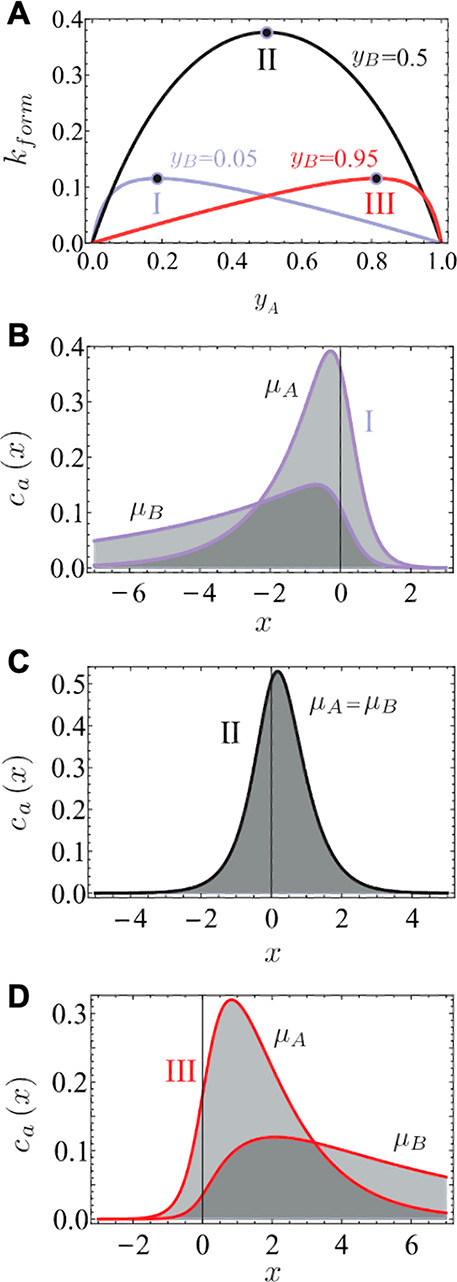
Analytical model predictions for the effect of reactant mobility on the rates of reaction accelerated using ITP. (A) Variation of the form factor k_form as a function of the mobility parameters of reactants y_A and y_B. (B–D) Concentration profile of reactants versus x corresponding to the parameters of points I, II, and III, respectively, in panel A. Figure was adapted with permission from ref (59). Copyright 2014 AIP Publishing.

In addition, Rubin et al.⁵⁹ also identified the time scale associated with ITP-aided reactions when the equilibrium constant is not negligible. In this case, the time to complete half the reaction τ̃_ITP scales as⁵⁹

113

Note that this scaling is different from τ_ITP for the case when k_off ≈ 0 (cf. eq 108). In the latter case, . The effect of k_off can be significant, especially at low analyte concentrations. For example, for standard DNA hybridization reactions with k_on ∼ 10⁴ M^–1 s^–1 and analyte concentrations on the order of 1 fM, Rubin et al.⁵⁹ found that reaction time scales for typical ITP conditions could be ∼10-fold lower when k_off took even a small but non-negligible value of 10^–4 s^–1 compared to the case when k_off ≈ 0.

Eid and Santiago⁶⁴ expanded aspects of the model of Rubin et al.⁵⁹ and explored the design of ITP systems that accelerate chemical reactions. They studied the effects of the initial sample placement (e.g., in the LE versus in the TE) on the influx rates of the reacting species and the associated product formation rates. Importantly, they identified that the amount (in moles) of product formed in ITP, N_AB, for time scales larger than the ITP reaction time scale τ̃_ITP is limited, in general, by the influx rates of the reacting species. Specifically,

114

Q_A^j and Q_B represent the influx rates of A and B into the ITP interface when initially loaded in the zone j (LE or TE). See Eid and Santiago⁶⁴ for a detailed discussion on parameters that govern influx rates in ITP. In the limit where species A is in excess compared to species B, N̅_AB^∞ approaches unity. In other words, the quasi-steady-state (i.e., for a sufficient reaction time) product formation rate in ITP is generally limited by the influx rate of the less abundant (limiting) reactant into the ITP interface.⁶⁴ Recently, Qi et al.¹⁹⁹ further expanded on the work of Rubin et al.⁵⁹ and Eid and Santiago⁶⁴ and studied the combined effects of species abundance and reaction off-rates on product formation dynamics in ITP. Specifically, they identified two key nondimensional parameters ϵ and v, which governed reaction dynamics in ITP, and studied regimes where the reaction was reactant- and kinetics-limited. Physically, ϵ represents the ratio of the reverse and forward reaction rates in ITP, and v represents the relative abundance (accumulation rate) of the reacting species within the ITP peak. Importantly, Qi et al.¹⁹⁹ observed that the amount of product formed in ITP under the quasi-steady state solely depends on v, while the time to reach the quasi-steady state is proportional to ϵ.

We have so far discussed homogeneous ITP reactions where both reactants focus in ITP. Eid et al.²⁰⁰ studied the case of homogeneous reactions in ITP where only one of the reacting species focuses and preconcentrates in ITP. A key nondimensional parameter that resulted from their analysis was a Damköhler-type number ,λ which represented a trade-off between reducing the assay time and increasing product formation. λ is given by²⁰⁰

115

where L₀ is the length of the channel. λ can be interpreted as a ratio between the advection time scale τ_adv that results from the electromigration of the ITP peak (which contains one of the reacting species) and the reaction time scale τ_rxn (which is governed by the abundant species, A). At low λ (i.e., when τ_adv ≪τ_rxn), the ITP peak migrates fast (i.e., low assay times) and the advective time scale is much smaller than the time scale for reaction completion, leading to minimal product formation in ITP. In contrast, for high values of λ (i.e., when τ_adv ≫τ_rxn), the reaction proceeds to near-completion over a time scale much smaller than that for ITP electromigration across the channel, leading to minimal effects of ITP on the reaction kinetics.²⁰⁰ Thus, desirable operating conditions should balance reaction completion and the assay time such that advective and reaction time scales are comparable (i.e., τ_adv ≈ τ_rxn). We here also note the work of Zeidman Kalman et al.,²⁰¹ who developed a detailed experimentally validated model for association–dissociation dynamics when only one of the reactants focused in ITP when the reverse reaction rate constant k_off was non-negligible. The unique dynamics associated with such reactions (for varying k_off) can be used to discriminate among specific versus nonspecific reaction products (e.g., for nucleic acid hybridization).

7.2. Theory and Models for Heterogeneous Reactions

We here discuss heterogeneous chemical reactions in ITP, which we define as those that involve at least one reactant immobilized to a surface or matrix within a microchannel while the other (solute) reactants electromigrate and focus in ITP. To a simple approximation, the reaction kinetics in such heterogeneous ITP reaction systems are governed by the interplay among transverse diffusion (diffusion to and from the surface), ITP peak advection, the kinetics time scale, and depletion effects. Consider that in such systems the immobilized reactant concentration is prescribed as a number density on the surface b_m with dimensions of moles per unit surface area, while the reactant that focuses in ITP has a concentration in dimensions of moles per volume c₀. The ratio of b_m and c₀ naturally provides a length scale that can be compared to the length scale normal to the immobilized reactant surface. We here suggest that a useful quantity is then the length scale of the dissolved-species reactant cloud, which must be “depleted” to completely saturate the surface. For a dissolved species in global abundance (relative to the surface reactant), this length scale is less than the channel dimension normal to the reaction surface, the channel depth h. For a low-abundance dissolved species, the maximum length scale for diffusion is the channel height, h.

Karsenty et al.²⁰² presented a model and scaling analysis for ITP systems involving heterogeneous reactions. They studied the reaction between target molecules focused in ITP and probe molecules immobilized on the surface of a microchannel (e.g., see Figure 14). They considered the limit where the diffusion time τ_D (τ_D = h²/D, where D is the diffusivity) across the channel depth was much smaller than the residence time of the ITP peak over the reaction surface (with the axial scale δ) τ_adv (τ_adv = δ/V_ITP), i.e., τ_D ≪ τ_adv. Further, they argued that the concentration of target molecules c_a in ITP remained nearly constant while electromigrating over the length l of the surface probes (i.e., Δc_a/c_a ∼ k_onb_ml/hV_ITP ≪ 1) and the system was kinetics-limited (not diffusion-limited).^202−204 These scaling arguments allowed them to model the concentration profile of an ITP-focused target as a top-hat function with a characteristic target concentration value (determined by the ITP preconcentration factor) and a characteristic width δ that travelled at V_ITP.^202−204 Paratore et al.²⁰³ later termed this simple operation method wherein ITP focused the target molecules as they electromigrated over surface probes as the “pass-over” (PO) mode. Karsenty et al.²⁰² described the reaction kinetics for the PO mode in terms of the following differential equation for the concentration of surface probes bound by the target b(t).

116

where τ_on^–1 = αc₀k_on (α is the ITP preconcentration factor and c₀ is the reservoir target concentration) and b_m is the total number of surface probes (free and bound). The reaction time scale τ_R in eq 116 is given by

117

where K_d = k_off/k_on. Note that α = 1 corresponds to the standard flow conditions without ITP. For the PO mode, the fraction of the bound probes (b_PO/b_m) versus the ITP residence time and kinetic rates was obtained from eq 116 as^202−204

118

where τ_PO is the duration that the ITP peak passes over the surface probes. Defining τ_tot as the total assay time (includes focusing, preconcentration, and reaction), Karsenty et al.²⁰² obtained the following enrichment factor from ITP compared to standard flow conditions:

119

An upper bound for ITP enrichment R is obtained at low concentrations and for τ_PO,τ_tot ≪ τ_off, and the enrichment factor is equal to ατ_PO/τ_tot. In the limit of high concentrations compared to the equilibrium constant, R approaches unity and ITP is not beneficial. A major limitation of the PO mode is that only a small fraction of target molecules (for example, Karsenty et al.²⁰² reported ∼1%) react with surface probes due to the short incubation time of the ITP peak over the probes relative to the advection of the ITP peak.

Figure 14.

Schematic representation and raw experimental images of the ITP-based surface immunoassay from Paratore et al.²⁰³ (A) ITP focuses target proteins and delivers them to the site where the surface reaction occurs. (B) Schematic of the acceleration of the reaction between surface-immobilized capture antibodies and the proteins focused (in solution) in ITP, which can be achieved using three modes. In pass-over ITP, the ITP peak electromigrates continuously past the surface reaction site. In the stop and diffuse mode, the electric field is temporarily turned off when the ITP peak is over the reaction site, and the peak is allowed to diffuse away from the reaction site with time. In counterflow ITP, a pressure-driven counterflow is used to hold the ITP peak stationary over the reaction site. (C) Detection is achieved by measuring the labeled antibodies bound to the reacted targets. The figure was reproduced with permission from ref (203). Copyright 2017 American Chemical Society.

Subsequently, Paratore et al.²⁰³ presented novel operation methods and associated models to improve the overall reaction efficiency of ITP heterogeneous reactions (cf. Figure 14). They introduced two new operating methods for ITP reactions, which they termed “stop and diffuse” (SD) and “counterflow” (CF).

In the SD method, the applied voltage is turned off when the ITP peak is over the surface probes, and the focused target is allowed to diffuse (and broaden) while reacting with the probes for some long duration. Paratore et al.²⁰³ studied the limit where the diffusion time scale across the depth was much smaller than the depletion time due to the surface reaction, an ITP peak width that was smaller than the reaction site, and a kinetic regime where the surface probes were far from saturation and the on-rate dominated the reaction kinetics. For this regime, Paratore et al.²⁰³ found the following analytical expression for the fraction of surface probes bound to the target in SD mode (b_SD/b_m):

120

where

121

In eqs 120 and 121, τ_dep = h/b_mk_on and τ_Dx = δ²/D, where h is the depth of the channel and δ is the ITP peak width. For long times t≫ τ_dep,τ_Dx, the bound fraction of the surface probes approaches a value of χαc₀. The SD mode is especially beneficial for the binding of large molecules with low diffusivities, such as proteins or antibodies, since low-diffusivity species retain the higher bulk concentration (due to ITP preconcentration and low diffusivity) for a longer time.²⁰³

To further improve the reaction efficiency, Paratore et al.²⁰³ considered counterflow (CF) ITP wherein the electromigration velocity of the ITP peak containing the targets is balanced by pressure-driven flow in the opposite direction such that the ITP peak remains stationary above the reaction site. They modeled reaction kinetics for a dispersion-free CF mode and derived the following expression for the fraction of bound surface probes (b_CF/b_m) for time scales greater than the depletion time scale:

122

where τ_acc = x_s/V_ITP is the electromigration time of the target from the reservoir to the ITP peak. Note that for the standard flow-through reaction the bound fraction scales as ∼k_onc₀t. Thus, the gain factor for the CF mode is proportional to ). This gain factor can be tuned by adjusting ITP focusing conditions such as the electric field strength, buffer concentrations and pH, and channel geometry.

Lastly, Shkolnikov and Santiago²⁰⁵ developed a numerical and analytical model for volumetric homogeneous reactions that involves the coupling of ITP and affinity chromatography (using a custom functionalized porous column). They used the model to predict spatiotemporal dynamics associated with the coupled electromigration, diffusion, and affinity reaction problem and to evaluate key figures of merit, including the capture efficiency, the assay time, and required length of the capture region. Importantly, they identified key limiting regimes of operation and obtained three nondimensionalized parameters that collapsed the dynamics. The first parameter was a Damköhler number that described the ratio between the electrophoretic time scale and the reaction time scale. The second parameter was the equilibrium constant nondimensionalized by the initial probe concentration. The last parameter represented the peak target concentration in ITP scaled by the initial probe concentration. We note that, in the latter case and the aforementioned cases of functionalized gels,^206,207 the time scales of diffusion to and from the immobilized species is negligible. Hence, the dynamics in such systems tend to be governed by competition between the advection time of the ITP zone and the reaction time scale. In these systems, diffusion plays a role only in the balance between the nonuniform axial electromigration and axial diffusion inherent in ITP.

8. Practical Considerations and Limitations for Microfluidic ITP

In this section, we review several considerations, useful practices, and limitations in the design of microfluidic ITP systems. We discuss topics related to interface dispersion, electrokinetic instability, Joule heating, pH buffering, separation capacity, the trade-off between sample volume and sensitivity, the operation method, and channel materials.

8.1. Interface Dispersion and Electrokinetic Instabilities

As discussed in section 5, an ideal one-dimensional ITP interface can become distorted (or disrupted) due to dispersion associated with external pressure gradients, unsuppressed residual EOF, and electrokinetic instabilities (typically at high electric fields). These effects can strongly influence the resolution and sensitivity of ITP systems. We here briefly review these effects and approaches that can be used to mitigate such nonideal behaviors.

Residual EOF in the channel often causes nonuniform EOF between the migrating LE and TE zones, which leads to the generation of internal pressure gradients and interface distortion (see Figure 15). In systems where the EOF is significant, adding a high-molecular=weight neutral polymer such as PVP, HPMC, or PEO in the LE or TE buffers suppresses EOF via the dynamic coating of the channel walls and results in a stable ITP interface.^183−189 Among the polymers, PVP at a 0.5 to 1% concentration is the most commonly used approach for glass- and plastic-based microfluidic channels. In case the addition of PVP results in undesirable sieving effects, the combination of a silanol coating such as Sigmacote and a surfactant such as Triton-X 100 is an effective alternative solution to suppress EOF, especially for borosilicate glass channels.³⁴ See Dolník¹⁸⁹ for a comprehensive review on various dynamic and permanent wall-coating approaches used in microfluidics to suppress EOF, including for channels fabricated using PMMA, polycarbonate, PDMS, and glass materials.

Figure 15.

Schematic depicting the curvature of the interface between the LE and adjusted TE zones at two different locations in the microchannel. An axially nonuniform electric field results in nonuniform EO slip velocities in the two zones. The latter leads to the generation of internal pressure gradients, which can lead to a distorted ITP interface. The figure was reproduced with permission from ref (61). Copyright 2011 Cambridge University Press.

In addition to EOF, pressure-driven flow can also disperse the ITP interface. This can arise from , for example, residual pressure-driven flow due to imbalances in the volume of liquid in the reservoirs or processes that are designed to include counter-pressure-driven flow in ITP.⁶⁰⁻⁶² Another source of pressure-driven flow can be random bubble formation processes at the electrode tips in the reservoirs due to electrolysis and the resulting differential gas generation at the two electrodes.²⁰⁸ Consider that 2 mol hydrogen gas is produced at the cathode for 1 mol oxygen produced at the anode. Effects due to such pressure differences can be mitigated by the use of gel-based plugs composed of buffer in agarose¹⁶² or Pluronic F-127 in the reservoirs.^204,209 Agarose melts at high temperatures, Pluronic F-127 is a liquid below 4 °C,²¹⁰ and both solidify and form gels when brought to room temperature. Next, note that instabilities in ITP can also occur due to differential Joule heating between LE and TE and internally generated temperature gradients, factors that result in a three-dimensional temperature field¹⁶² and secondary flow fields across the interface. Joule heating effects are discussed in section 8.2.

ITP as an electrophoretic process is characterized by an ion-concentration shock wave with self-sharpening gradients in the ionic conductivity and ion concentrations, which are primarily collinear with an applied electric field.^142,211,212 The sharp gradient in conductivity results in the accumulation of free charge at the moving ITP interface, which in turn couples with the local electric field and generates destabilizing electric body forces. This destabilizing force can disrupt the stability of the ITP interface and result in the dispersion of focused samples, which can lower the sensitivity of detection. Electric fields in microfluidic ITP are typically on the order of ∼1–10 kV m^–1 within channels of dimensions on the order of 10 to 100 μm. Typically, high electric field values are desired for ITP applications to improve the sensitivity and assay speeds. However, overly high electric fields can result in electrohydrodynamic instabilities,^70,213−215 and such effects can disrupt the sharp ITP interface and adversely affect the sensitivity.

Finite (including nonuniform) electroosmotic flow and pressure-driven flow (including counterflow) can cause dispersion of the ITP interface and lead to asymmetric profiles; existing numerical models and theories can predict some aspects of this behavior.⁵⁹⁻⁶² At high electric fields, the ITP interface can become significantly distorted and dispersed due to the onset of electrokinetic instabilities (EKIs, a regime of electrohydrodynamic (EHD) instabilities; see Figure 16).^124,216 The latter regime is characterized by unsteady three-dimensional fluctuations of concentration, the conductivity, and the electric fields near the ITP interface, which can lead to time-varying body force fields.

Figure 16.

Experimental visualization of an ITP peak at different time points in a straight-channel peak-mode ITP experiment. Images are shown for three different applied electric fields. Higher electric field strengths can lead to electrokinetic instabilities, which can distort the ITP peak. The figure was reproduced with permission from ref (124). Copyright 2009 IOP Publishing Ltd.

In general, EKI occurs when electric body forces dominate viscous forces in the flow. Posner and Santiago⁷³ summarized various formulations for the scaling of electric body forces relevant for EKI in terms of an electric Rayleigh number.^{182,217−219} Later, Persat and Santiago¹²⁴ presented a scaling for the electric body force ρ_eE at an ITP interface in terms of a modified electric Rayleigh number. Here, ρ_e is the free charge density at the ITP interface and E is the local electric field. Note that for typical EKI studies of symmetric binary electrolytes the length scale associated with the free charge is determined by convective-diffusive transport (not on the electric field). In contrast, for ITP, the length scales associated with free charge scale as the width of the ITP interface, which varies inversely with electric field. Persat and Santiago¹²⁴ thus report the scaling

123

where, E_avg = (E^L + E^T)/2 is the average of the electric field in the leading and trailing zones,and γ is the ratio between the leading and trailing zone conductivities. Importantly, this study strongly suggested an E³-type (stronger) dependence on the electric field for ITP compared to the E²-type scaling of typical other EKI studies.^{182,217−219} The study also suggested that the value of ρ_eE based on the above scaling empirically provides an upper threshold value of the electric field, which can be used to predict the onset of instability.

Later, Gaur and Bahga²²⁰ performed a detailed EHD instability analysis of a canonical single-interface ITP in an unbounded domain. They performed a linear stability analysis and showed that electroviscous flow destabilized ITP, while the electromigration of the shock wave had a stabilizing effect. Importantly, to quantify the effect of instability, they obtained a nondimensional number for the ITP in microchannels that was equal to the ratio of electroviscous flow time scale (τ_ev) to the restoring electromigration time scale (τ_em). The nondimensional number is expressed as

124

where μ_L is the electrophoretic mobility of the leading ion, E^L is the electric field in the LE, d is the (shallow) depth of the channel, ϵ is the dielectric permittivity, and η is the viscosity of the fluid. The ITP shock wave instability was found to set at low values of τ_ev/τ_em when the electroviscous flow dominated electromigration. Gaur and Bahga²²⁰ hypothesized that the exact value of τ_ev/τ_em below which ITP instability sets in depends on the channel geometry.

From eq 124, high values for the conductivity ratio, the channel depth, and the electric field promote instability, while high values for the fluid viscosity and the LE ion mobility have a stabilizing effect on ITP. In addition, the use of an array of posts²²¹ or porous structures¹⁸⁰ within the microchannels can increase the hydrodynamic resistance and stabilize the ITP interface. For example, van Kooten et al.²²² optimized and fabricated a microfluidic chip for ITP with an array of cylindrical pillars, where the pillars reportedly served to suppress the dispersion of the ITP interface due to potential spatial instabilities. The micropillars reduced the characteristic lateral dimension for viscous effects and conferred overall stability to the moving ITP interface.

Goet et al.²²³ also reported instabilities in the context of ITP with emulsions. They studied the ITP focusing of oil droplets initially suspended in the LE and noticed that the ITP peak formation exhibited vortical flow structures. They attributed these vortex structures to the body force on the droplets generated by space charge density at the interface. They hypothesized that the electric body force was balanced by the Stokes drag²²⁴ on the droplets within the ITP interface and developed a scaling approximation for the rotational velocity u_rot, where u_rot ∝ E² (E is the applied electric field). The model and scaling of Goet et al.²²³ is perhaps applicable to systems that involve the ITP focusing of micrometer-sized particles and beads.^224,225 Interestingly, in their bead-based ITP hybridization assay, Shintaku et al.²²⁵ deliberately operated at moderately high electric fields to utilize such secondary flow and vortex structures (see the video in the SI of that reference). This improved mixing of reagents enhanced the hybridization efficiency of the reaction between probe-functionalized beads and nucleic acid targets that cofocused in ITP. The latter study demonstrates that instabilities in ITP at moderate-to-high electric fields can be beneficial, especially for assays that require the efficient mixing of focused analytes involved in chemical reactions.

Lastly, note that the distortion of the ITP interface due to instability is reversible. Specifically, a stable interface can be quickly reestablished by lowering the electric field.^204,222

8.2. Joule Heating and Temperature Effects

Joule heating is ubiquitous in electrophoresis systems, including ITP, and can lead to the disruption of separation processes.^108,162,226 Joule heating is also the likely the most significant impediment to scaling up microfluidic ITP systems to process large sample volumes.^91,227 Further, the requirement to mitigate temperature increases in the microchannel due to Joule heating in ITP can strongly influence both chip design and assay time.^{179,222,228−230}

In ITP, the LE and TE zones have high and low conductivities, respectively. The volumetric heating rate (and temperature change) due to Joule heating is inversely proportional to the conductivity for a fixed current density. Further, the instantaneous current density is, to a very high accuracy, approximately uniform through the channel at any one time. Hence, LE and TE zones necessarily experience different Joule heating rates. The LE region is typically cooler than the TE zone, and there is an associated jump in temperature between the two migrating zones (see Figure 17).^{114,162,227,231,232} This feature has been employed for the thermometric detection of zone boundaries (cf. section 10.3). In general, the temperature increase due to Joule heating is function of the applied current, the ionic and thermal conductivities of the electrolyte, the thermal coupling of the channel to external environment, and the channel geometry. Moreover, the liquid is hotter near the center (interior) of the channel than the surrounding regions near the walls and reservoirs (in the absence of external heating), which results in nonuniform temperature fields within the cross-section (Figure 17). There are several detailed numerical and theoretical models that predict temperature fields in ITP.^{114,231−233} The temperature fields with the LE and TE evolve both spatially and temporally, with high temperature gradients occurring near the ITP interface.^114,162,232 Nonuniform temperature fields within the channel cross-section can also lead to internal secondary flow (e.g., due to buoyancy and electrothermal effects), which can significantly disperse the ITP interface (Figure 17A).¹⁶²

Figure 17.

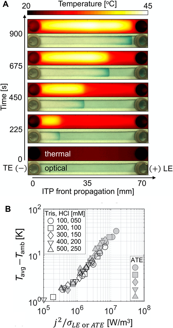
(A) Optical and thermal images of the ITP process vs time in a straight microchannel. Optical images show the focusing of a dye in peak-mode ITP and help track the LE–TE interface. Thermal images show spatial temperature fields in the channel. The temperature is significantly higher in the adjusted TE zone compared to that in the LE. (B) Spatiotemporal averages of the quasi-steady-state temperature increase from ambient temperature within the LE and adjusted TE zones as a function of the estimated volumetric Joule heating rates (proportional to the square of the applied current density). The figure was reproduced with permission from ref (162). Copyright 2020 Elsevier.

A passive approach to mitigate Joule heating effects is to use high-aspect-ratio channels (wide channels with shallow depths) to maximize the contact surface area of the liquid with the top and bottom channel walls and decrease the channel center-to-wall distance to enable efficient heat transfer.²³³ For channels with aspect ratios of perhaps three and higher, the difference in temperature between the center of the channel (T_cent) and the exterior walls (T_ext) due to Joule heating (in absence of external cooling) under a quasi-equilibrium steady state can be approximated as^179,233

125

The subscript i refers to the zone (LE and TE), h is the channel depth, d_wall is the thickness of the channel walls, and k_L and k_wall are the thermal conductivities of the liquid and the channel walls, respectively. The approximation and scaling in eq 125 assume negligible EOF or pressure-driven flow, i.e., there is negligible heat advection in the channel and the temperature field is predominantly governed by a balance between volumetric heating and heat conduction across the channel cross section. In other words, thermal equilibrium within the channel is achieved within the time scale of electromigration.²³⁴ Several studies^114,162,227 have experimentally validated the temperature scaling in eq 125 for ITP. For a given microchannel, ITP with higher ionic conductivity solutions (i.e., higher concentrations) and a lower current density results in a lower temperature change due to Joule heating. Note that higher current results in faster assay times and is in direct trade-off with Joule heating effects. Equation 125 can further be used to obtain an approximate expression for the maximum current, I_max, that can be applied in ITP due to constraints on maximum allowable temperature rise (ΔT_max).¹⁷⁹

126

Here, A_min is cross-section area of the channel and σ is the conductivity of the liquid at the “min” location, where “min” subscripts refer to locations along the channel where the product is the lowest. Equation 126 assumes negligible changes in material properties due to temperature. The value of ΔT_max depends, of course, on the application. For ITP applications involving proteins (e.g., immunoassays), the maximum operable temperature is typically less than around 40 °C to prevent protein denaturation. For ITP nucleic acids assays (e.g., hybridization reactions or on-chip ITP-mediated isothermal amplification), a higher temperature (e.g., 60 °C) might be desirable to provide stringency or optimize enzyme activity, which requires operation at higher currents. van Kooten et al.²²² and Terzis et al.¹⁶² demonstrated that temperatures of ∼65 °C could be achieved in ITP without overly disrupting the ITP interface (merely some additional dispersion). Higher temperatures due to Joule heating can lead to the degassing of buffers and significant bubble formation within the channel, which can disrupt ITP.

Another consequence of Joule heating is changes in buffer properties. For example, ion mobilities, ionic conductivity, thermal conductivity (of buffers and the chip material), the degree of dissociation, pH, and viscosity all change with temperature.^84,163 Of course, higher temperature changes result in larger changes of these thermophysical properties and consequently affect properties such as the ITP electromigration velocity and the electrical power required.¹⁶² These changes may sometimes be undesirable due to the need to preserve design characteristics of the electrolytes chosen for a particular ITP experiment. In addition to good channel geometry design (passive approach), active on-chip cooling mechanisms can be employed (e.g., Peltier cooling or contact with circulating cold water bath) to mitigate Joule heating effects.²³⁵

Lastly, we note that although Joule heating is usually an impediment in ITP processes, temperature changes and gradients associated with Joule heating in ITP may potentially be useful for certain applications. For example, Bender et al.²³⁶ leveraged the increased temperature (35 to 40 °C) in the adjusted TE zone that arose from Joule heating to simultaneously perform ITP and isothermal nucleic amplification using a method called recombinase polymerase amplification (RPA); see section 11.3 for more details.

8.3. Separation Parameter, Capacity, Charge, and Distance

Operation conditions and assay design parameters that optimize separations in analytical ITP applications have been well-studied in several works.^{2,85,244,168,237−243} An important concept in such system design is the so-called separation capacity, which plays a key role in regulating the efficiency of the ITP process.^237,238 The separation capacity is a measure of the amount of ions (e.g., moles of all ions in a sample volume) that can be processed by a given ITP process. Specifically, the separation capacity is a relationship between the amount of electrical charge required to be applied to separate and migrate a given amount and composition of the sample mixture. In this section, we will limit our discussion to the analysis of ITP figures of merit and design parameters relevant to the purification of sample analytes in peak-mode ITP (Figure 18). We refer to the studies of refs (2), (85), (243), (168), (194), and (237−242) for detailed discussions around optimization and design parameters for ITP processes involving separations in plateau-mode ITP.

Figure 18.

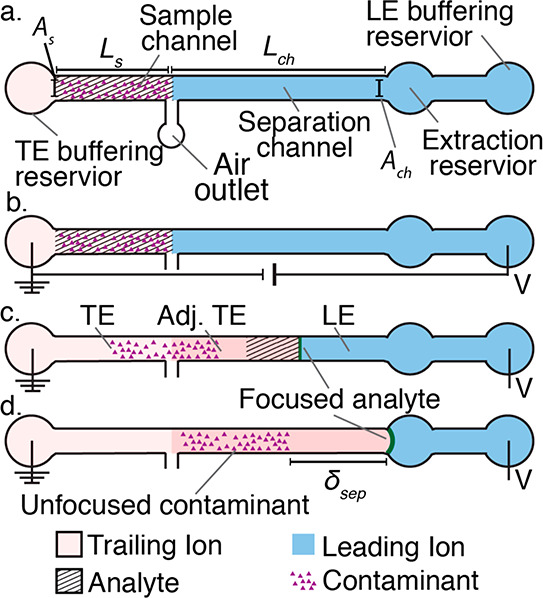
Schematic of an example system for ITP purification experiments. (A) Initial sample loading using finite injection. The sample is diluted in the TE prior to loading. (B) Application of an electric field in the main channel to initiate ITP. (C) Analytes focus in ITP while contaminants are left behind. (D) The experiment ends when the ITP peak (containing the analytes) reaches the extraction reservoir. Purified analytes are eluted from the extraction reservoir. The figure was reproduced with permission from the author of ref (179).

The discussion presented here follows the general approach of Boček et al.,²³⁸ which was originally developed for separation of ITP zones (plateau-mode ITP) and later expanded by Marshall¹⁷⁹ for peak-mode ITP purification applications and weakly ionized species. Marshall¹⁷⁹ considered an ITP problem of the purification and elution of a dilute analyte ion with a relatively high mobility from a sample that contained impurity ions of lower mobility. Marshall¹⁷⁹ considered the system shown in Figure 18, where the sample mixture is injected in a finite region between pure LE and TE buffers over a channel length L_s (and cross section area A_s), which is followed by a separation channel of length L_ch (and cross section area A_ch). Marshall considered a simple ITP process free of applied bulk flows.^{180,221,242,245−247} Further, for simplicity, Marshall studied a system with five ionic species comprised of a desired trace analyte, the highest-mobility trace impurity ion, leading and trailing electrolyte co-ions, and a counterion common to the LE and TE zones. The analyte and impurities were assumed to be in such low concentrations such that they did not significantly alter the zone conductivities or the pH. Such systems are common, for example, in ITP applications for the purification of nucleic acids or proteins from biological samples, which may contain several impurities and inhibitors for downstream analyses.³¹ Marshall further proposed a minimum set of design chip aspects for such applications that included air outlet sections to aid finite injection in addition to extraction and buffering reservoirs. The relations presented below assume that the raw sample is diluted in the TE during finite injection. We refer to Marshall¹⁷⁹ for results for the condition wherein the sample is diluted in the LE.

A key figure of merit relevant to purification processes is the recovery efficiency of the desired analyte from the sample. Recovery efficiency can also be formulated in terms of a separation capacity and a separation parameter.^179,238 Marshall obtained the number of moles of the focused analyte N_A per unit applied charge Q as

127

where c_A and c_T are the concentrations of the analyte and trailing ion, respectively; p_AT = (μ_A – μ_T)/μ_T is the separability parameter between the analyte with effective mobility μ_A and the TE co-ion with effective mobility μ_T;¹⁷⁸T_T is the transference number of the trailing ion (i.e., the fraction of total current carried by the TE co-ion);²³⁷ and λ_T is the molar conductivity of the trailing ion. The molar conductivity λ_i and the effective mobility μ_i of species i can be obtained as λ_i=∑_zμ_i,zg_i,zFz and μ_i = ∑_zμ_i,zg_i,z, respectively, where μ_i,z and g_i,z are the absolute mobility and the molar fraction of species i in charge state z, respectively. Note that the parameters in eq 127 are evaluated in the adjusted TE (ATE) zone, which is the newly formed TE zone formerly occupied by the LE. Ions in the ATE zone are subject to the appropriate regulating functions.⁷⁸

The separation parameter Q_s is equal to the amount of applied electric charge required to accumulate N_A moles of analyte at the ITP interface.^179,237,238 The total electrical charge Q_s required to extract all analyte ions from the sample can be obtained by setting N_A equal to the total analyte content of the raw sample and integrating eq 127 to give

128

where the subscript s indicates that N_A is being evaluated in the initial sample zone. Further, Marshall assumed well-buffered ITP where the pH of all zones is nearly the same and the effective mobility of the ions and the concentration ratio c_T/c_A are nearly the same in both TE and ATE zones.^179,248 Under this assumption, Marshall obtained the separation parameter Q_s in terms of the amount of TE co-ions in the initial sample zone (assuming the sample is diluted in the TE) [N_T]_s as

129

Equation 129 is more useful than eq 128, since the number of target analytes is often unknown a priori while the TE ion concentration (used to dilute the sample) is a design parameter easily controlled by the user. Further, note from eq 129 that the separation parameter Q_s is dependent only on the initial number of TE ions in the sample (or LE ions if the sample is diluted in the LE¹⁷⁹) and the properties of the ATE (or the LE if sample is diluted in the LE¹⁷⁹). Recall that ATE properties are regulated by the LE.

In practice, the charge transferred to the ITP system prior to the end of experiment (i.e., when the ITP interface reaches the elution reservoir) is limited by the time it takes for the ITP interface to traverse the separation channel region. This limits the actual amount of charge that can transferred in an ITP experiment, Q_L, which is the separation capacity.^179,238Q_L is best expressed in terms of the LE properties as^179,238

130

where the subscript L refers to the LE co-ion and the variables in the bracket are evaluated in the separation region of the channel initially filled with the LE. Note from eqs 129 and 130 that, for a given ITP buffer chemistry, the separation capacity and the separation parameter are directly proportional to the number of ions in the separation and sample regions of the channel, respectively.¹⁷⁹

The recovery efficiency of the ITP purification η under finite injection conditions, defined as the fraction of analyte ions that accumulate in the ITP interface before the interface reaches the end of the separation region, is the ratio of separation capacity and separation parameter, obtained as¹⁷⁹

131

where R_vol = ∀_ch/∀_s is the volume ratio of the separation and sample channel regions, [c_L]_LE is the concentration of the LE co-ion in the separation region, and [c_T]_s is the concentration of the TE co-ion in the sample region. Eid and Santiago⁶⁴ later obtained the following expression for the recovery efficiency in the case of the semi-infinite injection of the sample in the TE, η_si:

132

where β is the ratio of the TE ion concentration in the ATE and TE zones, ∀_ITP is the volume of the channel swept by the ITP peak, and ∀_well is the reservoir volume. In the limit when only a small fraction of the sample is processed (e.g., when the reservoir to channel volume ratio is large), then η_si ≈ p_ATβ∀_ITP/∀_well.

Next, the separation time t_sep, defined as the duration for the ITP interface to traverse the separation channel, can be obtained by dividing the transferred charge by the applied current (in the case of constant-current operation). t_sep is given by

133

t_sep scales inversely with the applied current and is proportional to both the LE co-ion concentration and the separation channel volume. Recall here the importance of Joule heating in limiting the applied current (see section 8.2).

Marshall¹⁷⁹ further considered the separation of the focused analyte from trace amounts of background nonfocused co-ion impurities in the sample. For simplicity, the separation of the analyte from the fastest moving background impurity (with effective mobility μ_R, less than μ_A) was considered in the analysis. In this case, the contaminant of interest electromigrates with velocity U_R less than the ITP interface velocity U_ITP, which is given by

134

When the ITP interface reaches the end of the separation channel (e.g., defined by the location of some detector), the distance of the focused analyte from the contaminant δ_sep, defined as the separation distance, can be obtained as¹⁷⁹

135

Notice that when the sample is diluted in the TE, δ_sep depends only on the separability of the contaminant and the length of the separation channel. When the sample is diluted in the LE, δ_sep depends additionally on the amount of LE ions in the sample and separation channels and the separability of the LE co-ion with respect to the contaminant.¹⁷⁹ Marshall¹⁷⁹ also presented an expression for the extra charge Q_ex that can be supplied to the ITP system between the time of arrival of the LE–ATE interface and the arrival of the leading contaminant. Q_ex is given by

136

In other words, Q_ex is the maximum additional charge that be applied to the system beyond Q_L to avoid any contaminants in the extraction reservoir. This extra charge may be useful, for example, to help move and guide the purified analyte within the extraction reservoir to enable efficient elution for off-chip analyses.

Another figure of merit for ITP purification is the sample dilution factor, F_dil.¹⁷⁹F_dil is defined as the ratio between the concentration of the target analyte in the raw sample and that in the extracted liquid. F_dil can be obtained in terms of the recovery efficiency η_f and the initial sample (∀_s) and extracted (∀_extract) liquid volumes as¹⁷⁹

137

In practice, ∀_extract depends on the extraction reservoir geometry and design and the liquid handing techniques used in the system.

8.4. Well-Buffered ITP Systems

This section presents some comments around the pH buffering of ITP experiments. pH buffering is important to ensure stable and/or functional (e.g., enzymes) biological species. pH buffering is also important for reproducible ITP processes, since weak electrolyte effective mobilities and solubilities depend on the local pH (as well as the ionic strength and the temperature). Of course, effective mobilities of species influence the conductivity and couple with the applied current (or voltage) to determine ITP front velocities. In turn, these quantities determine the system separation efficiency and accumulation rates. In this section, we will discuss two main aspects of buffering in ITP. The first is the chemical choice of the buffering ion(s) and titrant(s) among the anionic and cationic species of the LE and TE buffers. The second is the requirements (in particular, the volume and concentration) of reservoirs required to promote stable and reproducible system performance. Our discussion will assume the reader has a basic working knowledge of pH buffers, including buffer capacity, and familiarity with common buffering species (e.g., Good’s type buffer ions) and common titrants (e.g., chloride and sodium). See refs (76) and (77) for a detailed tutorial on pH buffers, including the coupling among ion mobility, ion velocity, and pH. We will also assume typical pH ranges of, say, 4–10 and buffers of sufficient ionic strength such that the safe pH and moderate pH assumptions apply.

8.4.1. Choices for Buffer Species

Our goal is to ensure the pH buffering of the LE and TE zones and, ideally, the pH buffering of plateau-mode zones. Note that we do not need a separate strategy to ensure the buffering of a trace species being focused in peak-mode species, as the distribution of pH (as well as the conductivity and the electric field) within such peaks is governed by the pH values of the neighboring plateaus. There are several approaches to ensure stable and reproducible pH values in an ITP process. We will here discuss what is, to our knowledge, the most widely applicable and reproducible method: buffering all zones using the LE counterion as the single buffering ion. The counterion of the original LE buffer is continuously supplied to the system by the LE reservoir. After sufficient time, the counterion from the LE zone displaces whatever counterion was in the original TE and so, eventually, the LE’s counterion is the only counterion in the adjusted TE region. The most straightforward method to ensure good pH buffering is then to make the LE counterion serve as the system’s buffering ion and the LE, adjusted TE, and any plateau-mode co-ionic species act as titrants to this buffering ion. Figure 19A and B demonstrate this arrangement for anionic (top) and cationic (bottom) ITP. Although not shown in the Figure 19, we consider the analyte X to be introduced via finite injection. In the top (bottom) schematic, the weak base (weak acid) migrates in the opposite direction of the LE anion (cation), eventually replacing the original cation (anion) in the initial nearby TE zone. Downstream, we observe that the adjusted TE is composed of the co-ionic TE anion (cation) and the weak base (weak acid), which migrates from LE to the ATE. To ensure well-buffered LE and ATE zones, we can choose an LE counterion with a convenient pK_a as the buffering weak electrolyte. Hence, in creating the LE buffer, we titrate this weak electrolyte using the other LE ion as the titrant. For anionic (cationic) ITP, we titrate the LE weak base (weak acid) using the LE anion (cation) as a titrant. For strong electrolyte univalent ion titrants, strong buffering is achieved when the titrant concentration is roughly half the concentration of the weak electrolyte. This 1:2 ratio also holds for weak electrolyte titrants with pK_a values roughly 1.5 pH units greater (lesser) than the pK_a of the buffering weak acid (weak base) (see Persat et al.⁷⁶ for the design of buffers using weak electrolyte titrants).

Figure 19.

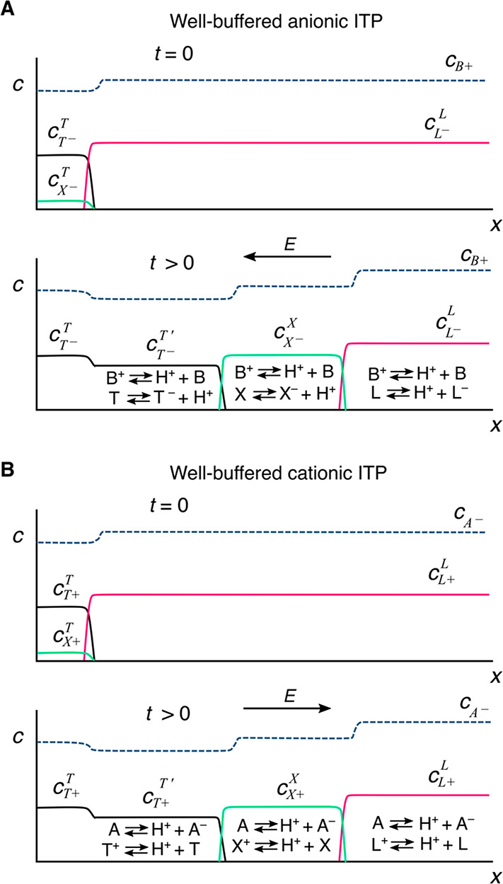
Schematic of well-buffered (A) anionic and (B) cationic plateau-mode ITP. Each subfigure depicts the concentration distributions of ions at the initial (top) and steady-state (bottom) separation conditions. Within each zone, the associated acid–base chemical equilibrium reactions are shown. A common weak base B (weak acid A) was used to buffer all zones in the anionic (cationic) ITP, as indicated by dashed lines. Although not shown here, the analyte X is considered to be introduced via finite injection.

As discussed in section 4, the concentration of the ATE co-ion will be on the same order as, and typically just smaller than, the LE co-ion. If we apply this section’s conservation principles to the counterion (which we leave as an exercise for the reader), we can show that the counterion’s concentration in the ATE will be roughly the same as its concentration in the LE. Hence, we expect the LE and ATE to each be buffered mixtures with a pH approximately the same as the pK_a of the weak electrolyte counterion (originating from the LE). Similarly, any plateau zone will be buffered near the pK_a of the counterion if the plateau species is an acid (base) with a pK_a at least about 1.5 pH units below (above) the pK_a of the weak base (weak acid) counterion. In summary, the idea is that the TE ion and the ions of any plateau zones in the system act as titrants to the LE buffer’s buffering ion. A common example system, applicable to a wide range of biological applications, is an anionic ITP process created using Tris and chloride as the LE buffer and Tris and HEPES as the TE buffer.^31,63,94,162 In creating the LE buffer, the analytical concentration of Tris is set at about twice the that of chloride. Conservation principles (see sections 2 and 4) then ensure that Tris enters the ATE at roughly twice the concentration of HEPES. Hence, Tris is the buffering counterion, with chloride and HEPES as titrants in the LE and ATE, respectively. The two zones are then well=buffered with a pH near the pK_a of Tris. In Supporting Information section S2, we provide general guidelines and a few recommendations on choosing ions and designing buffers for ITP.

8.4.2. Reservoir Buffering

All ITP is driven by Faraday reactions at electrodes. For microfluidics, these are nearly always electrodes inserted into end-channel reservoirs where electrolysis occurs. These reservoirs are typically open to the atmosphere to accommodate hydrogen (oxygen) gas generation at the cathode (anode). Importantly, the buffering capacity of the reservoir chemistry needs to be sufficiently strong to resist pH changes associated with electrolysis (i.e., acid and base generation at the anode and cathode, respectively).

A properly designed ITP system requires reservoirs with sufficient buffering capacities relative to the amount of charge injected into the system by the electrodes. The relevant proper design of reservoirs is discussed in detail by Persat et al.⁷⁷ and is merely summarized here. See the example system of Figure 20A. This figure considers a generic electrokinetic experiment where the current is driven by two end-channel electrodes though a microchannel. The species A and B in the diagram refer to generic “acid” and “base” ions of a buffer. As an example, consider A to be chloride ions migrating into the anodic reservoir (which is buffered by Tris). In this anodic reservoir, the pH drops over time as more charge is applied to the system. The drop in pH at the anodic reservoir is rapid if the initial pH is less than the pK_a of the weak base B, namely Tris (cf. Figure 20B). Likewise, the counterion Tris (weak base B in Figure 20A) migrates to the cathodic reservoir and increases the pH of the cathodic reservoir. However, the increase in pH at the cathodic buffer (Figure 20C) under the same conditions is more gradual.

Figure 20.

(A) Schematic depiction of a generic on-chip electrokinetic system where the electrolyte is a solution of a weak base B titrated with a strong acid A. (B and C) Predicted variations of the pH at the anodic and cathodic reservoirs vs time, respectively, due to electrode reactions. A Tris–HCl buffer system was considered, and a 100 μL reservoir volume was assumed. Shown are model predictions for various initial titrations of the pH of the buffer within one pK_a unit of the weak base Tris. The figure was reproduced with permission from ref (77). Copyright 2009 The Royal Society of Chemistry.

These observations lead us to another important consideration in the design of buffers in ITP, which is related to the buffering capacity (or buffer index), β. β represents the ability of the buffer to resist changes in pH and, as we discuss below, is proportional to the amount of applied charge.^76,77 β can be expressed as the amount of strong base or acid required to induce a small change in the pH of a weak electrolyte buffer, i.e., β = −∂c_A/∂pH (for the addition of strong acid A) or β = −∂c_B/∂pH (for the addition of strong base B). β is a property of the buffer and is a complex function of the ionic strength, pKa, temperature, charge transferred by the electrodes (equivalently, the duration of the experiment), and electrode reservoir volume.^76,77 For example, for the common example of a buffer composed of a 2:1 molar ratio of a weak base and a strong acid, β ≈ 0.56c_B, where c_B is the concentration of the weak base. For a given buffering capacity β and small pH changes (less than one pH unit), the applied charge Q is directly proportional to the change in the pH (ΔpH) and the buffering volume ∀_buf as follows:^76,77,179

138

Equation 138 can be used to estimate the maximum transferable charge Q_max for a maximum tolerable pH change in ITP (a design parameter), say, ΔpH_max, for given a reservoir volume ∀_buf.¹⁷⁹ Typical recommended values for ΔpH_max are around 0.2 to 0.4. Note further from eq 138 that a larger reservoir volume and a higher ionic strength allow for more charge to be transferred to the system while ensuring stable pH (see also the inset of Figure 20C).

Furthermore, anodic and cathodic buffers can also be designed by “anticipating” pH changes. For example, in anionic ITP, the pH of the anode (cathode) can be titrated such that the solution pH is slightly above (below) the pK_a of the weak base (acid). Similar strategies can be applied to cationic ITP systems.

Lastly, we note that atmospheric carbon dioxide dissolved in buffers can, in some cases, lead to unwanted side reactions⁸¹ and byproducts (e.g., carbamate and carbonate), which may result in the formation of additional (undesirable and unknown) zones during ITP.⁸⁰ For example, dissolved carbon dioxide can react with buffer species containing primary amines to form carbamate, which has a relatively high anionic mobility and focuses just behind the LE.⁸⁰ To mitigate the effects of carbon dioxide and related species, barium hydroxide has been mixed with the TE prior to chip loading to precipitate out dissolved carbon dioxide.⁸⁰

8.4.3. Operational Regime Map

The design of buffers is particularly important for the case of relatively large fluidic channels used to process relatively large reagent volumes (or relatively large reagent ionic strengths). As one instructive design process, see the work of Marshall¹⁷⁹ and Marshall et al.,²³⁰ who considered the combined constraints of the maximum permissible amount of electrical charge transferred (for stable pH buffering) provided by eq 138 together with system limitations imposed on the current magnitude by Joule heating (as a function of the LE concentration) (eq 126) and bubble generation at the electrodes due to electrolysis. These constraints were combined to create an “operational regime map” useful in system design (Figure 21). Contour lines represent achievable extraction times as functions of the applied current and the LE concentration (and the separation capacity in Coulombs). Shaded areas in the plot are precluded by design constraints and result in unstable operation. Such operation maps can be used to guide design trade-offs among assay time, the volume processed, the maximum allowable temperature achieved, and robust operation, including repeatable electrolysis bubble release.

Figure 21.

Example operational regime map for ITP purification experiments performed on a custom microchip designed by Marshall et al.²³⁰ Contours of the extraction time as a function of the LE concentration and the applied current are shown. Shaded regions are precluded by design and operational constraints. A low LE concentration results in high Joule heating. At high currents, large bubbles form at the electrode surface, leading to a poor electrical connection. Electrolysis can change the pH in the electrode reservoirs at a high separation capacity. The figure was reproduced with permission from Marshall et al.²³⁰ Copyright 2014 Elsevier.

8.5. Other Considerations for Practical ITP Experiments

There are, of course, many of other considerations associated with electrokinetic experiments and the design and operation of microfluidic devices.²⁴⁹ In this section, we briefly mention a few considerations particular to ITP experiments, including operation with constant current or constant voltage, trade-offs between sample volume and sensitivity, and channel materials.

ITP experiments are typically performed using either constant-voltage or constant-current operation. In channels of uniform cross-section operated at constant current, the system voltage typically increases linearly with time (since the total resistance of the channel increases as TE ions displace LE ions), while the ITP velocity is nearly constant. In this case, ITP dynamics are easier to analyze since, for example, finite injection samples will achieve a steady-state condition (in the frame of reference of the moving ITP interfaces). Experimentally, constant ITP interfaces are easier to track in space and time. Typical applied current values (e.g., using ionic strengths on the order of 100 mM) are a few microamps to tens of microamps for channels with cross-sectional areas on the order 100–1000 μm² and on the order of milliamps for cross sections on the order of 0.01 to 0.1 mm². In constant-voltage operation, the current and ITP-front velocity decrease with time (see the Supporting Information document of Bahga et al.¹²¹). Compared to constant-current sources, constant-voltage power supplies are generally more widely available and simpler and offer higher maximum voltage and power (compared to constant-current supplies). Typical values of applied voltages for ITP channels with lengths on the order of centimeters are on the order of 0.1–1 kV. It is important to estimate the maximum voltage and current requirements of an experiment. One approach is to perform preliminary experiments where the channel(s) is filled with either pure TE buffer or pure LE buffer and then perform simple current versus voltage calibrations of the channel. A nonlinear dependence between voltage and current in such experiments is indicative of Joule heating and, for large amounts of injected charge (compared to charge in buffered wells⁷⁷), can also indicate insufficient reservoir buffering (cf. section 8.4).

Another consideration is the amount of sample volume that can be processed on the chip. Electrokinetic microfluidic chips are generally designed to handle low sample volumes, typically on the order of few hundreds of nanoliters to a microliter. Larger volumes (and, in particular, channels with larger cross-sectional areas) are more difficult because of the constraints of Joule heating. However, larger sample volumes are sometimes required such as in the case of biological samples with trace concentration targets, which can require the processing of volumes on the order of 10–100 μL of raw sample (or larger). A common approach in such cases is to employ channels with high-aspect-ratio cross-sections, typically a large width and a small depth (along the vertical direction). Such channels are very compatible with microfabrication techniques and imaging and can offer larger volumes while mitigating Joule heating. Example ITP chips for processing relatively large volumes include those of Marshall et al.²³⁰ and van Kooten et al.,²²² which processed, respectively, 25 and 50 μL. A recently developed commercial device (IONIC ITP system, Purigen Biosystems, Pleasanton, CA) developed an injection-molded ITP chip to process 200 μL. There are, of course, systems that aim to both process large volumes and achieve high focusing and high plateau resolution. A classic approach to this is so-called column-coupled ITP, which employs a T-junction between a tube with a large cross-sectional area (for upstream volume processing) and a tube with a smaller cross-sectional area (for downstream high resolution).²⁵⁰ Tapered-area channels are also used in microfluidics for similar purposes.^121,251 In addition to the aforementioned methods, EOF or pressure-driven hydrodynamic counterflow can also be used to improve the throughput and amount of processed sample in relatively small volumes (although sometimes at the cost of longer assay times), a topic we review in section 12.

Lastly, we note that ITP microfluidic channels are typically fabricated from glass, fused silica, plastics or, less frequently, paper-based materials. Glass microfluidic chips are available from several vendors. Some examples include Caliper Life Sciences (a PerkinElmer company, MA), Micronit (Netherlands), and Microfluidic ChipShop (Germany). Common polymers used are PMMA,³⁰ polycarbonate,²⁵² polystyrene,²⁵³ cyclic olefin copolymer (COC),²³⁰ and elastomers, particularly PDMS.^26,204 Paper-based ITP systems are typically fabricated using nitrocellulose,^254,255 glass fiber,²⁵⁶ or the proprietary Fusion 5 membrane materials.^256,257 Recently, 3D printed microchannels were fabricated for ITP applications.²⁵⁸ A few important considerations for choosing channel materials include the low surface adsorption of the target molecules, the ability to sustain a high voltage prior to breakdown (e.g., silicon channels are rarely used for ITP for this reason), amenability to surface functionalization (e.g., for surface-based ITP reaction assays), stable thermal properties, high thermal conductivity and diffusivity (e.g., as offered by glass), and compatibility with precision fabrication and microfabrication methods. We refer to refs (259−264) for comparisons and detailed discussions around various channel materials useful for on-chip electrophoresis applications, including ITP.

9. Brief Review of Simulation Tools

The theory presented in the above sections does not always allow for simple analytical calculations associated with the ITP process. Computer simulations have therefore played an important role in bridging the gap between theory and practice and have greatly aided in the design and optimization of microfluidic ITP systems. Note, however, that simulating ITP dynamics can be computationally challenging since it is a highly nonlinear process that involves multiple chemical species, chemical equilibrium reactions, sharp gradients in concentration, coupling with electric fields and, at times, coupling with bulk flow. Significant improvements have been made in the modeling and simulation of electrokinetic processes over the last three to four decades. In this section, we briefly review simulations tools useful for ITP, with an emphasis on those which are publicly available. As we shall see below, 1D dynamic simulators are at present the most widely used design tools for ITP. We note, however, that complex ITP phenomena (e.g., dispersion) and channel geometries (e.g., nonuniform cross-sections) may require simulations that are area-averaged, 2D, or 3D for better accuracy.

9.1. One-Dimensional ITP Simulation Tools

The earliest studies on numerical simulations of electrophoretic processes in general include the related works of Bier et al.,²⁶⁵ Saville and Palusinski,⁷⁹ and Palusinski et al.²⁶⁶ Bier et al.²⁶⁵ were the first study to implement any kind of an electrophoresis code applicable to ITP. In later (related) publications, Saville and Palusinski⁷⁹ and Palusinski et al.²⁶⁶ presented generalized formulations for electromigration–diffusion–advection processes that included multiple weak electrolytes (including ampholytes with univalent ionization states) and provided a unified framework for simulating a variety of electrokinetic processes, including ITP. Thereafter, several improvements in the physical modeling of electrokinetic processes were suggested and implemented in numerical codes and simulation software packages, as mentioned below. Some of the key improvements include adaptive grid techniques to efficiently resolve high-concentration gradients,^78,142 effects of ionic strength on species mobility and ionic activity,^144,169 Taylor–Aris-type dispersion to account for sample dispersion in the presence of nonuniform EOF or pressure-driven flow,^78,267 axially varied channel cross-sections,^268,269 and the simulation of complex-formation equilibria^37,270 and nonequilibrium chemical reaction kinetics.²⁷¹

At present, commonly used dynamic electrophoresis simulation packages for modeling microfluidic ITP include SIMUL,¹⁴⁴ GENTRANS,^{79,265,266,272} and SPRESSO.^78,121,169 These software programs are largely based on the theoretical formulation of Saville and Palusinski,⁷⁹ and have been periodically (and significantly) updated to include new computational capabilities and physical models such as those mentioned earlier. In 2009, Bercovici et al.⁷⁸ introduced a Taylor–Aris-type dispersion model to account for sample dispersion in the presence of nonuniform EOF and pressure-driven flow in the SPRESSO software. In a similar vein, GENTRANS was later expanded by Caslavska et al.²⁶⁷ to include Taylor–Aris-type dispersion effects. GENTRANS was also expanded by Breadmore et al.³⁷ to include calculations involving electrokinetic chiral separations with a neutral ligand. A similar extension of SIMUL 5 was presented by Hruška et al.²⁷³ and Svobodová et al.,²⁷⁴ which led to SIMUL 5 Complex software. Dagan and Bercovici²⁷¹ extended SPRESSO to include nonequilibrium homogeneous and heterogeneous reaction kinetics of chemical species. Ionic strength effects, which are typically modeled using the Onsager-Fuoss model¹⁷³ and the extended Debye–Hückel theory¹⁷⁴ for ionic activity, were included originally in SIMUL 5¹⁴⁴ and later implemented in SPRESSO by Bahga et al.¹⁶⁹ Recently, the software SIMUL 6²⁷⁵ was launched as a successor of SIMUL 5. SIMUL 6 uses parallelization and multithread computation to significantly speed up the computation time compared to SIMUL 5. In 2021, Avaro et al.²⁷⁶ published an open source, web-based, and cross-browser-compatible ITP simulation tool called CAFES. CAFES enables rapid computations of the dynamic ion concentration and pH fields during ITP for a wide range of sample injection configurations. It has a built-in database of buffer ions but also enables custom-designed buffer mixtures. CAFES has a simple graphical interface for user inputs, and the simulations are directly performed on the user’s computer (by their browser software), requiring absolutely no prior installation or compilation of the software.

The aforementioned 1D simulators are strictly applicable only to straight channel 1D ITP. Hence, they predict only streamwise variations in the concentrations of species and cannot account for spanwise (and transverse) variations in concentration, for example, due to dispersion or cross-sectional area changes. The latter requires two- or three-dimensional simulations, which we discuss in section 9.2. However, Hruška et al.²⁶⁸ and Bahga et al.¹²¹ used area-averaged 3D species transport equations to approximate the effect of cross-sectional area variation in 1D. They, respectively, expanded SIMUL and SPRESSO to include a quasi 1D model to account for cross-sectional area changes in the channel. As an illustration, Figure 22 depicts the present capabilities of the SPRESSO software.

Figure 22.

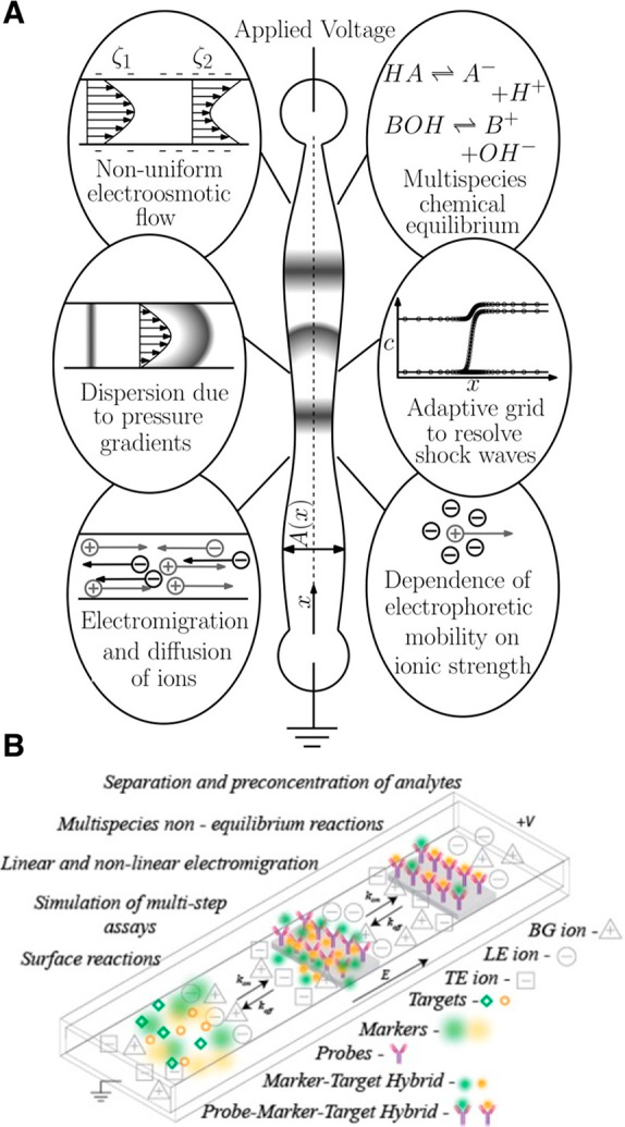
(A) Schematic highlighting the various physical features of the SPRESSO simulation tool developed in refs (78), (142), and (269). The figure was reproduced with permission from ref (269). Copyright 2012 John Wiley and Sons. (B) Illustration of the extended version of SPRESSO by Dagan and Bercovici,²⁷¹ including a chemical reaction module that simulates electrophoresis-driven hybridization, binding, or chemical reaction processes. The figure was reproduced with permission from ref (271). Copyright 2014 American Chemical Society.

SPRESSO is freely available for download from http://stanfordspresso.blogspot.com/. GENTRANS is available upon author request (from wolfgang.thormann@ikp.unibe.ch). CAFES simulations can be performed for free at https://microfluidics.stanford.edu/cafes. We note that PeakMaster is another often used electrophoresis software, but it is only applicable for zone electrophoresis (and provides a rapid way of determining buffer equilibria and species mobility). The latter software is based on the linear theory of electromigration. Both SIMUL and PeakMaster software packages can be downloaded for free from https://web.natur.cuni.cz/gas/.

Further, we note that although the underlying physical models are largely common among the simulation software and several other numerical studies of ITP, the numerical methods (in particular, the spatial discretization scheme) used are significantly different. The choice of the numerical method determines the trade-offs among computational speed, accuracy, and spatial resolution. It is instructive to broadly categorize the numerical schemes (based on the spatial discretization) as dissipative or nondissipative. Dissipative schemes use numerical diffusion to provide a stable nonoscillatory solution at the expense of low accuracy (e.g., they predict a much larger interface width than is physical). Examples of dissipative schemes include the upwind scheme,²⁷⁷ the flux-corrected transport scheme,²⁷⁸ the space-time conservation element solution element scheme,²⁷⁹ and the symmetric limited positive scheme.²⁶⁹ In contrast, nondissipative schemes offer higher accuracy at the expense of increased computational time. Nondissipative schemes typically require a higher number of grid points to prevent oscillatory solutions. Examples of such schemes include the second-order central difference²⁷² and sixth-order compact schemes.⁷⁸ Additionally, as mentioned above, numerical schemes that use adaptive grid refinement⁷⁸ (e.g., SPRESSO) or those based on pseudospectral methods²⁸⁰ have shown improvements in computational time and accuracy. The latter pseudospectral method was recently developed by Gupta and Bahga²⁸⁰ for electrophoresis simulations, including transient ITP (t-ITP), and was released as a free software package called SPYCE, which can be downloaded at https://web.iitd.ac.in/~bahga/SPYCE.html. We refer to refs (281−283) for studies that directly compare the performance and accuracy of several 1D simulators across various electrophoretic processes, including ITP. Lastly, we mention a free open-source software tool called STEEP that enables detailed calculations of temperature effects of ionic species mobility and pH equilibria.¹⁶³

9.2. Multidimensional ITP Simulation Tools

As mentioned above, ITP in microfluidic channels can strongly exhibit two- and three-dimensional concentration fields, for example, in the presence of a streamwise variation in the channel geometry or due to dispersion associated with pressure-driven flow or EOF. Additionally, complex sample injection strategies²⁸⁴ and ITP processes very often involve microfluidic chips with branched channel networks,³⁶ and these require at least 2D simulations to model the underlying electrokinetic transport. To study such effects, researchers have mostly relied on multiphysics software packages, which include COMOSL Multiphysics^{61,180,251,270,285} (COMSOL, Inc., Burlington, MA), CFD-ACE+^284,286 (CFD Research, Huntsville, AL), and the freeware OpenFOAM.²⁸⁷ For example, Garcia-Schwarz et al.⁶¹ and Schönfeld et al.¹³⁹ used COMSOL to study 2D fields associated with sample dispersion in ITP due to nonuniform EOF. Likewise, GanOr et al.⁶⁰ and Liu and Ivory²⁸⁸ used COMSOL in 2D to study the effects of counterflow in ITP. Paschkewitz et al.²⁸⁹ used CFD-ACE to study ITP focusing in serpentine passages in a microfluidic chip.

In addition, custom numerical codes have also been developed to simulate and study ITP processes in 2D. For example, Bhattacharyya et al.⁶² developed a third-order QUICK scheme to study sample dispersion in the presence of a counterflow in ITP. Likewise, Shim et al.²⁹⁰ developed a finite-volume solver to study a five-component ITP system.

To our knowledge, the only study to date that reports the 3D simulation of ITP is the work of Bottenus et al.²⁵¹ They used COMSOL to simulate 3D ITP sample focusing and preconcentration in a cascade microchip, which had a channel cross-sectional area that decreased 100-fold along the streamwise direction. It was later reported that this simulation took several weeks to complete.¹⁹

Though insightful, the main drawback of using multidimensional tools to simulate ITP is the computational cost. At present, 2D simulations take several hours to days, while 3D simulations require several weeks or longer, depending on the computational power and memory. In contrast, 1D simulations can take seconds to minutes to run and can be performed on personal computers. For this reason, we believe that 1D dynamic simulators will continue to play an important role, at least in the near future, for quick ITP assay designs, including buffer chemistry, injection, initial configuration, operating electric field, detector placement, and overall optimization (including trade-offs among resolution, sensitivity, and assay time).

10. Experimental Tools and Detection Methods

In this section, we begin by providing scaling arguments for the resolution and sensitivity of separation processes that use plateau-mode ITP. We then review various methods used for experimental visualization and analyte detection in microfluidic ITP. We place special emphasis on fluorescence, thermometric, and conductometric detection approaches, as these are the most compatible with microfluidic devices. Additionally, we focus on detection systems for analytical ITP and do not review methods that couple ITP purification, focusing, and separation with downstream analyses such as zone electrophoresis, mass spectroscopy, or chromatography. See refs (22), (24), (242), and (291−294) for discussions on the latter topic. Also refer to https://microfluidics.stanford.edu/resources for a series of ITP tutorial videos showing protocols for carrying out on-chip ITP experiments including buffer and chip preparation, electric field control, and imaging.

10.1. Sensitivity and Resolution for Plateau Zones

The width of plateau regions, Δx_i, is proportional to the amount of analyte i collected (eq 95). These widths, and the widths of the interfaces between plateaus, δ, therefore determine the minimum amount of analyte that can be detected via plateau identification. The step heights in the signal plateau regions, Δs_i, are related to differences between the effective mobilities of the analytes and that of the LE. For example, an analyte mobility much lower than that of the LE will cause a large step height.

In the plateau mode, we can therefore define the sensitivity, S, as a measure of whether an analyte that forms a local plateau region can be differentiated from both of its two adjoining plateaus. Well-resolved peaks will have plateaus widths Δx_i much larger than the interface width between zones δ (cf. Figure 16). Hence, we recommend that S can be formulated as

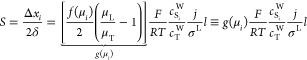139

Here, g(μ_i) is a function of the mobilities (between the square brackets of eq 139) and, as an estimate, we have used the expression for the boundary width δ from eq 45. We see that for a given applied current, decreasing the leading ion conductivity increases the electric field overall and decreases the interface width, thereby increasing the sensitivity. Of course, sources of dispersion (e.g., unwanted pressure gradients) would result in larger interface widths than our simple diffusion-only model used here (and hence reduce the sensitivity).

Next, in the plateau mode, we can define resolution, R, as our ability to detect the mobility of one analyte versus another. To do so, we should have a sufficient signal difference, Δs, relative to the LE ion (whose mobility is precisely known). This signal difference can be compared to background signal noise σ_s (cf. Figure 23) as follows

140

Figure 23.

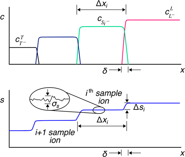
Schematic depicting typical (A) concentration vs x and (B) generic detector signal s vs x (equivalently, time) plots for fully formed and separated plateau zones for an arbitrary number of analyte species S_i. The length of the i^th plateau zone is indicated by Δx_i, and the interface width between successive zones is indicated by δ. σ_s is a measure of the noise of the detector.

As an example, for a monovalent strong electrolyte sample initially loaded in the TE, the signal difference Δs scales as

141

From eq 141, we see that an increased LE concentration results in a stronger signal difference. This is because a high c_L^L yields large absolute values of signal throughout all ITP zones, and the resolution R scales as the difference (in the units of the signal) between these absolute values. The noise of plateau signals, σ_s, is determined by several factors, including the noise in the detector (e.g., due to amplification or readout noise) and spatiotemporal variations in background signal.

Overall, for plateau-mode ITP, the analysis presented above suggests that decreasing c_L^L (thereby decreasing LE conductivity σ^L) increases sensitivity S, while increasing c_L increases resolution R. A simple approach to improve sensitivity is to use tapered channels wherein the detection region has a smaller channel cross-sectional area, as has been demonstrated by several studies.^{121,251,269,295} This is because a smaller cross-sectional area (like decreasing the conductivity) increases the electric field for the same applied current. Bahga¹²¹ presents analytical expressions for the plateau length as a function of the local cross-sectional area in an ITP channel.

10.2. Fluorescence Detection

Fluorescence-based detection is very attractive for on-chip microfluidic applications due to its ease of implementation and high sensitivity and the fact that it is a contactless approach. Microchannels typically have good optical access (e.g., channels made from glass or plastic) and sufficiently low background fluorescence (albeit with a short optical path length) for sensitive fluorescence detection. Fluorescence detection can be used to directly detect fluorescent analyte species or to indirectly detect analytes using nonfocusing tracers,³³ fluorescent mobility markers,¹⁰⁶ or fluorescent carrier ampholytes.¹⁰⁵ We will review these methods in more detail below. In principle, direct and indirect detection approaches are both applicable in the detection of both peak and plateau mode analytes. However, in practice, direct detection is typically used for peak-mode analyte detection, while indirect detection is used to identify separated analyte zones in the plateau mode. Key components of fluorescence-based detection include a light source (e.g., LED, laser, or mercury bulb), optical filters, microscope optics, and a detector (e.g., CCD and CMOS cameras or pointwise detectors such as PMT and a photodiode). Fluorescence detection systems are possible in various formats, including miniaturized and portable systems compatible with microfluidic systems.

10.2.1. Direct Detection

In the direct detection approach, fluorescent molecules are directly focused in ITP and detected. The species of interest are either natively fluorescent (e.g., inherently fluorescent proteins and molecules) or fluorescence-labeled (e.g., SYBR-based labeling of nucleic acids or fluorescent-tagged proteins) prior to or during ITP. Some of the earliest demonstrations of direct fluorescence-based detection in ITP were in the works of Reijenga et al.,²⁹⁶ Kaniansky et al.,²⁹⁷ Schmitz et al.,²⁹⁸ and Jarofke.¹⁵³ Reijenga et al.²⁹⁶ combined simultaneous fluorescence detection and UV absorption in ITP to directly detect quinone in soft drinks and bovine serum albumin. Kaniansky et al.²⁹⁷ used ITP and fluorescence measurements to detect as low as 250 fmol amino acids labeled with 2,4-dinitrophenyl. Likewise, Schmitz et al.²⁹⁸ prestained lipoproteins with a fluorescent lipophilic dye called 7-nitrobenz-2-oxa-1,3-diazole-ceramide and detected them using ITP from human serum samples. Jarofke¹⁵³ used ITP to detect up to 3 ng mL^–1 fluorescent histamines.

Fluorescence detection methods gained significant popularity in the late l990s with the rapid growth of microfabrication techniques and significant improvements in the sensitivity of optical detectors, and they have been widely employed in ITP.^{245,299−303} Direct detection can be used to visualize or track plateau zones as well as the interface region between zones (e.g., using a fluorescent molecule that focuses in the peak mode between two consecutive plateau zones). This is useful, for example, for extracting trace analytes such as nucleic acids from raw biological samples (see Figure 24C),^32,92,94 or before they interact with downstream zone electrophoresis (ZE) to improve resolution.³⁰ It can also be used for the highly sensitive quantification of trace amounts of analytes and to estimate the degree of preconcentration in ITP.^111,304 We discuss the physics around the manipulation and detection of trace analytes in peak-mode ITP in section 5 and mention applications and achievable LODs in section 11. Direct detection of the ITP peak, especially using spatial detectors such as CCD and CMOS cameras, also provides access to detailed two- or three-dimensional information on the shape of the focused species. This has led to a new fundamental physical understanding of the ITP processes and has been useful in the development of methods to minimize sample dispersion for in-line quantification.^{61,62,222,230} For example, see the optimized chip design and associated ITP visualization in Figure 24A from the study of van Kooten et al.²²² As another example, Khurana and Santiago⁹⁸ and Garcia-Schwarz et al.³⁴ (see Figure 24B) quantified the scaling and relations among peak-mode width, sample concentration, and current using fluorescence imaging of AF488 dye in peak-mode ITP. In the same vein, Garcia-Schwarz et al.⁶¹ and Bhattacharyya et al.⁶² measured 2D depth-integrated peak shapes in ITP using fluorescent species to study the mechanisms underlying sample dispersion in ITP. Direct fluorescence readouts have also been useful in the design of several ITP-enhanced chemical reaction assays that require the monitoring, separation, and control of cofocused species.^{39,94,112,204} ITP-aided reactions are reviewed in detail in section 8. We also note here that, for millimeter-scale ITP devices, fluorescence visualization may be performed directly without the need for a microscope (of course, however, with the presence of an appropriate excitation light source and filters).^209,230

Figure 24.

Direct detection and visualization of peak-mode ITP in various microfluidic systems. (A) Fluorescence images of the peak-mode ITP focusing and preconcentration of dye SYTO9 at various axial positions in a custom large-volume PDMS–glass microfluidic chip. The figure was reproduced from with permission from ref (222). CC BY 4.0. (B) Peak-mode ITP focusing of the fluorescent dye AF488 vs various applied currents between 0.4 and 4 μA. Experiments were performed in a commercially available borosilicate glass microfluidic chip (NS12A, Caliper Life Sciences, MA). The figure was reproduced with permission from ref (34) Copyright 2012 JoVE. (C) Visualization of the ITP peak during the extraction, purification, and preconcentration of nucleic acids from a raw nasopharyngeal swab sample. Nucleic acids were stained using the fluorescent intercalating dye SYBR Green I. Experiments were performed in an NS12A Caliper chip (same as panel B). The figure was reproduced with permission from ref (94). Copyright 2020 National Academy of Sciences.

An obvious limitation of direct fluorescence detection in ITP is the availability of inherently fluorescent analytes or difficult with labeling analytes. Only a limited number of species offer native fluorescence in convenient wavelengths or contain functional groups such as thiols, free amines, or hydroxyls that enable derivatization.¹⁰⁶ The simultaneous detection of multiple species (in the same zone) can also be hampered by methods to discriminate among excitation and emission wavelengths simultaneously. This can be addressed to a degree using multichannel (i.e., different wavelengths) detectors, but multiplexing is often limited to 3–5 different channels. Another consideration is the dye photostability or the pH insensitivity of the fluorophore, which enables concentration quantification and assay reproducibility (e.g., unlike fluorescein, AF488 has excellent photostability, and its fluorescence is insensitive to pH for pH values above ∼4).^98,305 Interestingly, pH-dependent dyes have also been used to indirectly detect and identify species in ITP.^1,306,307 Lastly, note that the lower limit of detection of all fluorescent detection methods is limited by the detector noise and background auto fluorescence of the chip and reagents.

It is worth noting that most microfluidic ITP studies involving trace analyte detection have almost exclusively used fluorescence-based detection. This is due its high sensitivity, ease of implementation, and compatibility with standard microfluidic setups (cf. sections 5 and 11). Several strategies can be combined and used to optimize the sensitivity of detection in peak-mode ITP.^98,111 For example, the concentration of the focused analyte is proportional to the leading ion concentration, thus a higher LE concentration can enable an increased peak concentration. Likewise, a low TE concentration locally increases the electric field in the reservoir or initial sample zone and thus favors higher sample influx rates. In addition, semi-infinite sample injection allows for the continuous injection of the analyte into the peak and can be more beneficial than a finite injection mode for trace analytes. In a similar vein, counterflow ITP and increases in channel length can also used to increase the focusing time and the amount of sample focused in peak-mode ITP. Reducing the channel cross-sectional area also allows for a higher current density (by mitigating the effects of Joule heating) and can also be used to improve sensitivity.^121,188,308

10.2.2. Indirect Detection

In the indirect fluorescence detection (IFD) approach, nonfluorescent analytes are identified indirectly (with minimal or no a priori knowledge of the physicochemical properties) by adding nonreacting fluorescent tracer species.^{33,106,296,309,310} In IFD approaches, the fluorescence-labeled species are typically present in trace quantities in the LE or TE buffers and thus contribute negligibly to the local conductivity. This is unlike indirect detection methods that use UV absorption, where the concentration of UV-sensitive species is often on the same order of the buffering ions and can contribute significantly to the local conductivity.^{307,311−314}

We here can classify IFD methods into two broad classes. The first IFD approach, called the nonfocusing tracer (NFT) technique,³³ utilizes fluorescent species tracers that do not focus in ITP (but electromigrate) and whose fluorescence intensity varies and adjusts spatially depending on the physicochemical properties of the separated zones. This is schematically depicted in Figure 25. As discussed by Chambers and Santiago,³³ detection using the NFT approach can be achieved using fluorescent (nonfocusing) co-ions or counterions. The NFT ion can be either an overspeeder or an underspeeder. Overspeeders or underspeeders can electromigrate in the direction of the ITP wave but do not focus because they have mobility magnitudes that are higher than the LE ion or lower than the TE ion, respectively. When a fluorescent counterion NFT species is used, the ion is called a counterspeeder. The counterspeeder migrates from the LE to the TE, traversing all zones. Chambers and Santiago³³ also presented the theory around detection using the NFT technique. By conserving ion fluxes, they derived the follows expression for the concentration ratio of the NFT ion i in zone A (analyte A) versus zone B (analyte B) in terms of the effective mobilities of the species:

142

The second equality in eq 142 assumes that the fluorescence intensity is proportional to the concentration of the NFT species (which is valid in the absence of self-quenching^296,315). The mobilities in the expression are effective mobilities. Despite the striking similarity between eqs 142 and 79 (the latter equation represents adjusted concentrations of trailing zone analytes), it is important to note that the concentrations in eq 142 are necessarily trace quantities unlike the concentrations in eq 79, which are on the order of the buffering ions. Additionally, eq 142 holds true for both univalent and multivalent species. For a fully ionized high-mobility counterspeeder, the intensity ratio approaches the effective mobility ratio, i.e., I_A/I_B ≈ μ_A^A/μ_B. The sensitivity of counterion NFT is nearly uniform across all analyte mobilities. On the other hand, the most sensitive regime for co-ionic NFT is where μ_i^A ≈ μ_A, i.e., where the mobility of the analyte is nearly equal to the NFT. The NFT-based approach, like thermometric detection, is a fairly universally applicable method for plateau-mode ITP. Figure 25C is an example from Chambers and Santiago³³ which shows the NFT-based detection of HEPES and MOPS using the counterspeeder species rhodamine 6G (R6G). Garcia-Schwarz et al.³⁴ later demonstrated the separation and NFT-based indirect detection of two amino acids (arginine and lysine) in cationic ITP using R6G as an underspeeder. In a similar vein, Smejkal et al.³¹⁶ demonstrated the separation and detection of eight carboxylic acids using R6G as the counterspeeder.

Figure 25.

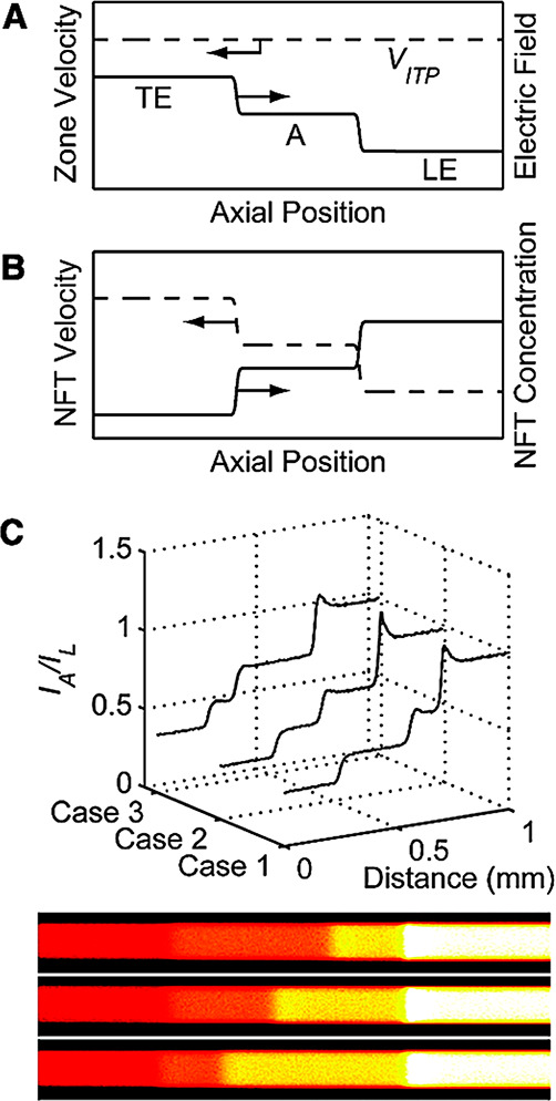
Qualitative representation of the indirect fluorescence detection method using a nonfocusing tracer (NFT) ion. (A) Depiction of plateau-mode ITP with a single analyte A under steady-state conditions. (B) Adjustment of the NFT concentration and velocity profiles within each zone. (C) Experimental detection of HEPES and MOPS in plateau-mode ITP using a counterionic fluorescent NFT rhodamine 6G. The top panel shows the ratios of the zone intensities (each zone intensity was normalized by the LE value), and the bottom panel shows the corresponding experimental images. Figure was adapted with permission from ref (33). Copyright 2009 American Chemical Society.

A major advantage of the NFT approach is that only a single fluorophore is required to detect multiple analytes. Drawbacks of the NFT technique is that self-quenching can become an issue at sufficiently high NFT concentrations (e.g., within the LE zone) and there can be undesirable chemical interactions between the NFT and the analytes (e.g., via complex formation).³¹⁷ Other challenges may include the adsorption of the dye to the channel walls (e.g., R6G is cationic and adsorb to negatively charged glass channel walls).³³

A second approach to IFD uses fluorescent mobility marker species.^{105,106,310,318,319} These are fluorescent spacer ions that focus between plateaus (including the LE and the TE) and thereby help determine the effective mobility of nonfluorescent analytes in plateau zones (see also refs (80), (318), and (320−322)). Khurana and Santiago¹⁰⁶ demonstrated this approach using a set of carefully selected fluorescent mobility markers (e.g., Oregon Green carboxylic acid, fluorescein, and Bodipy) for the indirect detection of amino acids and achieved a detection sensitivity of ∼10 μM. Their assay was limited by the possible number of fluorescent markers with appropriate mobilities required for separation and also had the disadvantage of requiring a careful a priori choice of markers depending for specific target analytes.

An analyst can use many fluorescent mobility markers to relax the requirement for a priori knowledge of the analyte mobility and to improve both the resolution and the dynamic range of potentially detectable species. A good example of this is the fluorescent carrier ampholyte assay (FCA) of Bercovici et al.^105,310 and Kaigala et al.³¹⁹ Carrier ampholytes are amphoteric small molecules, typically synthetic polypeptides with varying isoelectric points, and can aid separations in ITP.^323−326 The latter mixtures of hundreds or thousands of carrier ampholytes are typically used to establish a background pH gradient in isoelectric focusing experiments.³²⁷ In the FCA assay, this mixture was added to the ITP buffers, and many carrier ampholytes accumulated between the LE and the TE. Analyte ions (that are not fluorescent) present in sufficiently high concentrations displace these labeled ampholytes and create “gaps” in an otherwise contiguous (albeit nonuniform) fluorescence signal. Figure 26 shows the concept of the FCA assay. Integrating the fluorescent signal (e.g., from left to right) with and without analytes helps identify the fraction of ampholytes focused to the left or right of an analyte “gap” and hence quantifies the analyte effective mobility relative to the mobility distribution of the FCAs. The gap width quantifies the amount of analyte present (see eq 143).^1,195 As with the NFT approach, this approach can be used only for analytes present in sufficient concentrations such that they are at least near the plateau mode. Bercovici et al.³¹⁰ demonstrated this technique for the detection and quantification of four model analytes consisting of 20 μM MES, 40 μM MOPS, 30 μM ACES, and 50 μM HEPES (see Figure 26C). Bercovici et al.¹⁰⁵ also applied the technique to the label-free detection of 2-nitrophenol (2NP) and 2,4,6-trichlorophenol (TCP) toxins in tap water on a hand–hand portable ITP device (compatible with point-of-care) and achieved detection limits of ∼1 μM.

Figure 26.

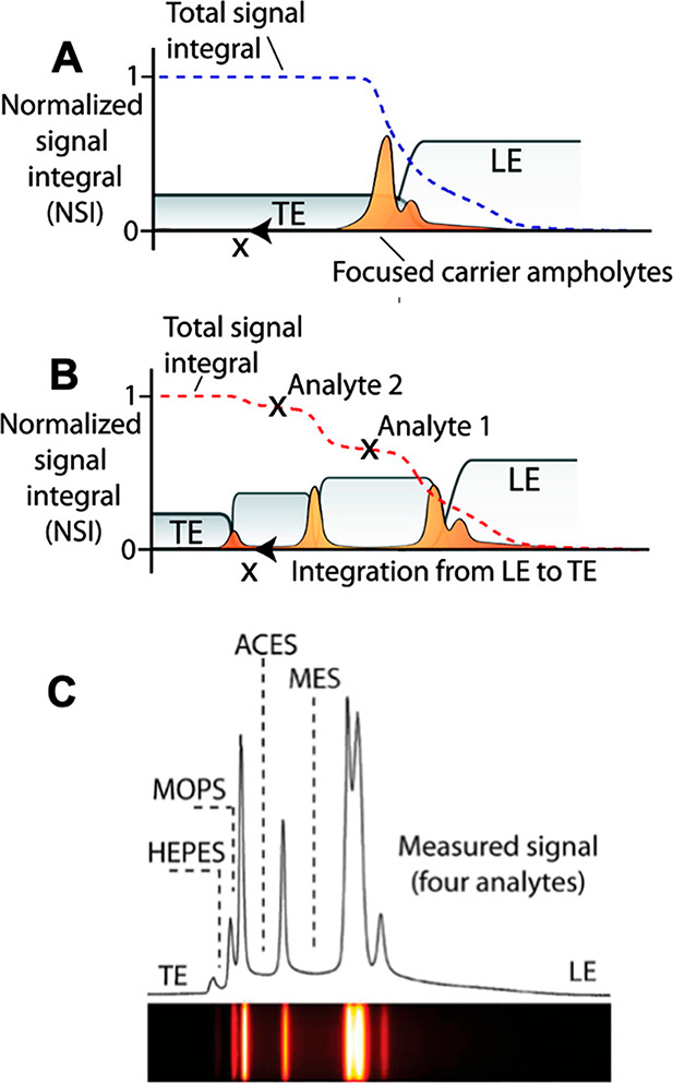
Schematic and experimental demonstration of the indirect detection of ITP separation using the fluorescent carrier ampholyte (FCA) assay. (A) All the labeled carrier amphoytes (CAs) focus at the LE–TE interface in the absence of the sample, resulting in a continuous fluorescence signal. (B) Analytes focused under ITP displace subsets of the labeled CAs, resulting in gaps in the measured fluorescence signal. Plateau regions in the normalized signal integral (NSI) indicate the presence of specific focused analytes. The NSI value can provide quantitative information about the effective mobility of the focused analytes. (C) Experimental demonstration of the FCA assay for the indirect detection of four analytes consisting of 20 μM MES, 40 μM MOPS, 30 μM ACES, and 50 μM HEPES. The heatmap of the raw signal (below) and the corresponding intensity profile (top) are shown. Figure was adapted with permission from ref (310). Copyright 2010 American Chemical Society.

10.3. Thermometric Detection

In ITP, the conductivity of the zones typically decreases from the highest value in the LE to the lowest value in the adjusted TE. This variation in conductivity affects both the volumetric Joule heating rate and the associated temperature increase within each electromigrating zone. The temperature within each zone typically achieves a quasi-steady-state equilibrium value, which is determined by the balance of heat conduction fluxes (away from the channel axis, through the liquid, and across channel walls) and the volumetric Joule heating rate (see more details in section 8).^{15,114,162,227} For a given local current density j, the local temperature increase ΔT within a zone scales inversely with the zone conductivity σ as ΔT ∝ j²/σ. Thus, the temperature increases (in a roughly stepwise fashion) from the LE to the TE zone (and across analyte zones), as shown by the experimental data in Figure 27. This variation in temperature over zones is the basis for thermometric detection in ITP.

Figure 27.

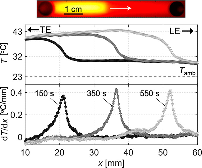
(Top) Heatmap of the experimental spatial temperature profile measured during ITP. Measurements were obtained using contactless infrared thermal imaging. (Middle) Plot of the spanwise-averaged temperature vs the channel length at three intermediate times during ITP. (Bottom) Plot of the temperature gradient versus the channel length at three intermediate times during ITP. Figure was adapted with permission from ref (162) Copyright 2020 Elsevier.

The temperature (and its gradients) can be measured using point-wise detectors such as thermocouples^1,17,18,157 and thermistors,^2,328,329 which are typically bonded to the exterior channel walls, by point-wise measurements of the differential absorbances of narrow-band diode lasers,³³⁰ or by contactless thermal imaging, for example, using an infrared (IR) sensor or camera.^162,179 Though early works used thermistors immersed in liquids,¹³⁴ such an approach is not recommended, since the sensor can itself disturb and interfere with the ITP process. Current thermometric detection approaches do not involve direct contact with the liquid in the channel. Such sensors rely on the assumption that a rapid thermal equilibrium is attained between the solution within the channel and the channel wall over time scales much smaller than the time required for the electromigrating zone to pass by the detector. We also note that temperature-dependent fluorescent dyes (e.g., Rhodamine B) exist that could, in principle, be used as an approach for thermometric detection in ITP. This approach has been used for other microfluidic applications,³³¹ but to our knowledge remains unexplored for ITP.

The thermometric detection method is a universal approach¹ (i.e., applicable to all species) because the measured temperature signal is a function of the conductivity (and consequently the constituent ion mobilities) of the separated zones that is not inherently species-specific. For this reason, this method cannot be used for peak-mode ITP, since the trace sample ions in peak mode contribute negligibly to the local conductivity. Note further that this method (and in general all universal detection methods, including thermometric and conductometric) cannot distinguish pure zones (consisting of single focused species) from so-called shared ITP zones (zones that contain a stable mixture of two or more species in a plateau).¹⁹³ We will limit our discussion here to the common case of the detection of pure zones.

To well-resolve zone boundaries using thermometric detection, the length scale of the zones of varying temperature l_T should be larger than the interface width δ between zones (i.e., a zone truly in the plateau mode, see section 7). l_T should also be larger than the characteristic integration length (along the channel axis) of the temperature sensor. Sharp changes in the measured temperature can be used to quantitatively estimate the lengths of the plateau zones. The measured zone length can, in turn, be related to the species concentration in the plateau, and one can infer the original analyte concentration from these data. For finite sample injection width l_inj of analyte X, which is focused into an ITP plateau zone of length l_X (measured) with steady-state concentration c_X^X (measured or predicted by a model or simulation), the initial injected analyte concentration c_X,inj can be obtained from species conservation as^1,195

143

where γ = S_det/S_inj is the area ratio between the detection and injection regions, respectively.^33,121 Note that this above relation is also applicable to fluorescence- (cf. section 10.2) and conductivity-based (cf. section 10.4) detection methods.

A limitation of pointwise temperature sensors such as thermocouples and thermistors is that they usually require more complex device fabrication or setup to achieve sufficient thermal contact with the wetted channel wall. Direct thermal imaging is much more versatile and provides spatiotemporal information within the entire field of view. One limitation of the latter is that IR cameras tend to have lower resolutions than visible-light cameras (one recent optical setup provided a resolution of 10 pixels mm^–1).¹⁶²

Generally speaking, the spatial resolutions of thermometric methods are poorer than those of methods based on UV absorbance or fluorescence.¹ Using thermometric detection, typical minimum detectable zone lengths are around 2–5 mm.^{1,108,227,328} The resolution of concentration value (via the accurate measurement of the plateau zone length) can be improved by increasing the time of separation, which results in longer plateau lengths (cf. sections 6 and 10.1). Lowering the LE concentration can also increase the resolution by proportionally decreasing the concentrations of trailing zones (this also increases the Joule heating for the same applied current density). The latter approach is, in turn, constrained by the minimum desired buffering capacity of the system at low ionic strengths and other problems associated with significant Joule heating (cf. section 8). Another limitation of thermometric approaches is that the temperature increases can depend on the thermophysical properties of the channel wall. Thus, temperature detection methods require the careful calibration for each different channel design and material if quantitative information is desired. Lastly, sensitive thermometric detection also requires that plateau zone conductivities be sufficiently different to result in measurable temperature differences The latter requirement may be a design trade-off with the need to maintain sufficiently low temperatures. High absolute temperatures can modify or damage analyte species (e.g., in bioassay applications), and high temperatures and temperature gradients can result in poor reproducibility or even unstable flow fields. A potential way to mitigate temperature effects is to ensure good thermostatic temperature control along the entire chip, particularly near the detection region.

10.4. Conductivity Detection

As discussed in sections 2–4, the conductivities of plateau zones in ITP vary in accordance with charge neutrality, species effective mobilities, and current continuity. Specifically, the conductivity typically decreases monotonically from the LE to the TE across zones, and the ratio of the conductivity between two generic zones A (species A) and B (species B) can be expressed in terms of the effective mobility and the concentration of the species as follows:

144

where subscript C refers to the counterion and the concentrations are the “adjusted” values governed by the Jovin and Alberty relations (cf. section 4). This variation is the basis for conductivity-based zone detection methods for ITP.^332−336 Note that the ratio in eq 144 also helps govern the temperature fields for thermometric detection (as discussed in section 10.3). Conductivity detection is a fairly universal method and can be used to detect ions that focus and segregate into plateau zones in ITP.¹ As with other techniques, conductivity methods provide information on the zone length, which is useful for quantifying the amount (or initial concentration) of analyte, as given by eq 143 (in addition to direct measurements of the zone conductivity). As with other methods, conductivity-based methods cannot be used to detect peak-mode analytes, since such ions contribute negligibly to the local conductivity.

Early applications of this method directly measured the conductance of the solution using sensing electrodes in direct contact with the solution within the channel and a high-frequency alternating current–voltage operation to avoid Faradaic reactions.^{1,168,337,338} This approach is currently disfavored because direct electrode contact with the solution can lead to undesirable bubble formation, polarization and unwanted passivation of the sensing electrodes, and signal interference from the high separation voltages in the main channel.^339,340 Moreover, in the direct contact approach, which was originally developed for capillaries with large inner dimensions, sensing electrodes were typically introduced into the channel through laser-drilled holes, which required complicated fabrication procedures. Direct contact is also less convenient and incompatible with the small channel dimensions typical of microfluidic applications. To address these limitations, in 1980, a new class of contactless conductivity detection methods was developed for capillary ITP systems by Gaš et al.³⁴¹ and later improved by Vacík et al.³⁴² Gaš et al.³⁴¹ demonstrated good reproducibility and better resolving power in ITP separations that used the contactless conductivity detection compared to those that used thermometric detection. It is also worth noting that the studies of Gaš et al.³⁴¹ and Vacík et al.³⁴² were among the earliest reported demonstrations of the contactless conductivity technique across all electrophoresis separation methods. Contactless conductivity methods were then significantly improved in 1998 by Fracassi da Silva et al.³⁴³ and Zemann et al.,¹⁰⁴ mainly geared toward capillary electrophoresis applications. The early 2000s saw several studies that developed novel microfabrication techniques for integrating contactless conductivity on-chip for ITP and several other on-chip electrophoresis applications.^{250,344−350} A notable example is the study of Graß et al.³⁵¹ from 2001, which was the first to describe the fabrication and testing of a fully integrated contactless conductivity detector on a poly(methyl methacrylate) (PMMA) chip for ITP separations. Figure 28C shows an example isotachopherogram for the separation and detection of oxalate and acetate based on conductivity measurements from the latter study.

Figure 28.

Depiction of and sample data for capacitively coupled contactless conductivity detection (C⁴D) detection for ITP separations. (A) Integration of planar electrodes for C⁴D on a microchip. Figure adapted with permission from ref (345). Copyright 2008 John Wiley and Sons. (B) Equivalent circuit model for a typical C⁴D microcell, consisting of the solution resistance R_s, the wall capacitance C_w, and a stray capacitance C₀. The figure was reproduced with permission from ref (347). Copyright 2012 The Royal Society of Chemistry. (C) Detection of the ITP separation of oxalate and acetate in a custom PMMA microfluidic chip using C⁴D. The figure was reproduced with permission from ref (351). Copyright 2001 Elsevier.

The contactless conductivity method, now commonly known as capacitively coupled contactless conductivity detection (C⁴D), typically uses high-frequency alternating current measurements between two (or four) closely spaced electrodes placed directly on or around the external surface of the microchannel. Hence, there is no direct electrode material-to-solution contact. This configuration can be achieved by either directly fabricating the electrodes on the chip (see Figure 28A) or by attaching an externally connected C⁴D cell in close proximity to the channel within a chip.^104,343Figure 28B shows a simple equivalent circuit model for a C⁴D measurement cell consisting of two electrodes (viz., excitation and sensing) separated longitudinally along the channel.³⁴⁷ The main circuit components include the solution resistance R_s, the wall capacitance C_w (since the wall acts as a dielectric layer in series), and a stray capacitance C₀ due to the direct capacitive coupling between the electrodes. See refs (104) and (335) for more detailed models, which include effects due to the electric double layer capacitance and the resistance. We refer to refs (352−357) for some excellent reviews on recent developments in the instrumentation, fabrication, and design of contactless conductometric detection methods for on-chip electrophoresis applications.

C⁴D modules are now available commercially and are commonly used as detectors for on-chip microfluidic ITP applications. For example, Cong et al.³⁵⁸ and Bottenus et al.³⁵⁹ used commercial C⁴D units to monitor the ITP separation of lanthanides on custom-built PMMA and fused-silica microfluidic devices, respectively. As another example, Koczka et al.¹⁸⁶ combined UV detection and C⁴D and performed ITP analyses on a variety of samples such as red wine, fizzy drink, and juice. The study of Koczka et al.¹⁸⁶ also importantly highlighted a major limitation associated with the resolution power of C⁴D systems. The resolving power of C⁴D systems is limited by the separation distance between the sensing electrodes (which is typically around 1 to 2 mm). For example, a separation distance of 1 mm requires that the ITP plateau zone width be greater than about 1 mm to achieve good resolution. Another major consideration for C⁴D is the requirement of a thin channel wall (on the side where the electrodes are placed), which is typically limited to a few 100 μm. A thinner wall enables better capacitive coupling with the solution in the channel and results in a higher sensitivity. Typical sensitivity values for C⁴D systems are in the sub-micromolar range.¹⁸⁶ It is also important to note that conductivity methods are currently limited to pointwise measurements in ITP, i.e., signal versus time can be measured only at a single or at most a few spatial locations along the channel. This is in contrast to fluorescence imaging or thermal imaging methods, which provide detailed spatiotemporal information.

10.5. Other Methods

We here briefly mention several other methods, including uncommon methods, applicable to on-chip ITP detection. A few of these methods have special historical significance as early approaches to ITP detection.

UV-based detection was widely used in early studies of ITP (both off-chip and on-chip). This method utilizes at least one species focused in (near-plateau-mode) ITP that exhibits significant UV absorbance.^1,103,360 For example, a UV-detectable counterion can be used to detect unlabeled species in plateau-mode ITP as it traverses from the LE to the TE and adjusts its concentration (and associated UV absorbance) across various zones.^296,361 Another implementation involves the use of UV-detectable spacer ions that form intermediate zones between non-UV-detectable (UV-detectable) analyte zones, thus enabling indirect (direct) analyte detection.^321,322 Of course, a straightforward application for UV-based detection involves the direct detection of analytes that significantly absorb light in the UV wavelengths.^129,362 Importantly, UV methods require concentrations of the UV-detectable species to be on the same order as that of the buffer (unlike fluorescence methods, which are applicable down to trace concentrations). Additionally, UV absorbance methods are often not very sensitive for microfluidic applications due to the small optical path lengths in the microchannels. Lastly, like the UV-based method, chromophores^186,363,364 and radioactive^365−367 species can also be used for detection in ITP (of course, using the appropriate detectors), although such methods usually have relatively low sensitivities.

Another class of detection methods is based on electrochemical measurements (amperometric,^368,369 potentiometric,^370−373 and potential gradient^374−376). Recall that the electric field and the conductivity vary across ITP zones and, respectively, increase and decrease monotonically from the LE to the TE. This effect forms the basis for electrochemical detection methods in ITP. These methods involve current or voltage measurements made locally in-line using the direct contact of source and sensing electrodes with the solution. In such methods, it is important that detection-associated measurements do not significantly affect the driving current or voltage supplied through the main channel for ITP separation. As mentioned in section 10.4, fabricating such systems with direct electrode contact with the solution can involve complicated procedures (rarely compatible with microfluidics) and can often lead to undesirable effects at the electrode surface (e.g., bubble formation, Faradaic reactions, and passivation).

Lastly, we note that it is generally challenging to visualize or detect nonfluorescent trace analytes in peak-mode ITP. In this regard, Karsenty et al. developed a method based on current monitoring within a channel, with multiple constrictions to detect the peak-mode sample location. In a different approach, Eid et al.³⁷⁷ used a fluorescence-tracking dye (AF647) compatible with their downstream assay to detect an ITP peak that contained nucleic acids. Interestingly, nonfluorescent dyes such as tartrazine and cresol red can also been used in the visualization of ITP experiments.³⁶⁴

11. Applications of Microfluidic ITP

This section summarizes various references that employ microfluidic ITP for practical applications. Applications reviewed here include the use of ITP for analyte purification, preconcentration, separation, reactions, and sensitive detection. We will place a special emphasis on bioassay systems involving ITP. The discussions are not meant to be comprehensive but instead to present examples aimed at indicating the variety of systems that have been explored.

11.1. Purification and Concentration of Trace Analytes for Sensitive Detection

ITP is a powerful purification and preconcentration tool that can be used for a variety of on-chip applications. We will here mostly focus on peak-mode ITP applications that involve the direct detection of trace analytes. ITP can also be used as a preconcentration step prior to separation using zone electrophoresis to improve the latter’s resolution and sensitivity, a topic we discussed in more detail in section 10.1. Some of the early demonstrations of the peak mode (called by some early researchers the spike mode) were performed in the late 1970s in capillary ITP systems in the work of Svoboda and Vacík³⁶⁰ and Everaerts et al.,³⁷⁸ where peaks in UV isotachopherograms were used for the direct quantitative evaluation of trace analytes involving organic weak acids. Picomolar levels of trace analytes were detected using this approach.

The years between late 1990s and early 2000s saw the first implementations of ITP in microfluidic chips.²⁵⁻³⁰ In several of these studies, ITP was primarily used as a preconcentration method in tandem with downstream separation using zone electrophoresis. Nevertheless, we briefly review below some of the ITP aspects of these studies, since these studies were among the earliest to demonstrate and quantify the degree of preconcentration achievable using peak-mode ITP. Wainright et al.³⁰ reported a ∼500-fold increase in the concentration of their fluorescence-labeled eTAG reporter molecules in peak-mode transient ITP performed in a PMMA microchannel. Their limit of detection was in the subpicomolar range of reporter molecules. Similar fold increases were reported by Jeong et al.²⁹ for ITP experiments involving fluorescein as sample, which were performed in a PDMS chip in around 2 min. In 2006, Jung et al.¹¹¹ reported the preconcentration of an AF488 sample on the order of a million-fold in a few minutes using peak-mode ITP performed on a commercially available glass microchannel. They detected initial sample concentrations as low as 100 fM. Later, Jung et al.³⁰⁴ implemented high-numerical-aperture light collection and a PMT to improve the sensitivity and reported the detection of an initial AF488 concentration as small as 100 aM. Sample preconcentration was also, more recently, demonstrated in a nitrocellulose paper-based microfluidic device by Moghadam et al.²⁵⁴ The latter group reported a 900-fold increase in the AF488 sample concentration in peak-mode ITP in ∼2 min (see Figure 29). Figure 29 also shows that the amount of sample focused in peak-mode ITP in their device increased linearly with time (see data for x/L_i < 0.6) for constant-current operation (as discussed in section 5.2). The deviation from linearity for x/L_i > 0.6 was attributed to dispersion due to nonuniform EOF.

Figure 29.

(A) Experimental images of the ITP preconcentration and focusing of an AF 488 sample in peak-mode ITP implemented on a nitrocellulose-based paper device. Snapshots taken at (i) 1, (ii) 30, (iii) 60, (iv) 90, and (v) 140 s after the application of the electric field. (B) Plot of the sample concentration normalized by the initial sample concentration (C/C_i) and accumulated moles of sample normalized by the initial moles of sample in the TE reservoir (N/N_i) versus the normalized axial length. Refer to Moghadam et al. for details on the experimental setup and the device design. The figure was reproduced with permission from ref (254). Copyright 2014 American Chemical Society.

Peak-mode ITP has also been used for other microfluidic applications and assays involving biomolecules such as nucleic acids and proteins. In such applications, ITP is typically used to simultaneously purify and preconcentrate target molecules from background contaminants and ions present in the raw biological samples, followed by either direct on-chip detection or downstream analysis (e.g., PCR). For example, Persat et al.³² purified and preconcentrated nucleic acids from whole blood using ITP and demonstrated the compatibility of the extracted volume with downstream PCR. Bercovici et al.³⁹ reported the preconcentration of nucleic acids in ITP on the order of 1000 to 10 000-fold. Similarly, Bottenus et al.¹⁸⁸ and Bottenus et al.²⁵¹ demonstrated the preconcentration of proteins in ITP on the order of 10,000-fold prior to on-chip detection. Refer to Rogacs et al.³¹ for a comprehensive review of the applications of microfluidic ITP for nucleic acid purification. We review such bioassay ITP systems in more detail in section 11.3. Preconcentration provided by peak-mode ITP can also be applied to initiate and accelerate chemical reactions involving molecules that focus in ITP, a topic we discuss in section 11.4. Lastly, refer to sections 10.2.1, 5, and S2 for discussions around methods to increase trace analyte focusing rates in ITP and improve the sensitivity.

11.2. Applications of ITP for Separations

Applications of ITP in microfluidics for separations can broadly be categorized into two types. The first type segregates (and therefore separates) co-ionic species into plateaus, and these are detected while the species are still in plateau-mode ITP. The second type uses ITP as an initial preconcentration process and then ends or disrupts ITP to effect a capillary electrophoresis-type separation. In this section, we shall concentrate on the first type. We summarize the second type in section 12.

Separation and detection while still in the ITP mode require that all analytes of interest necessarily form plateau zones. These zones can be detected either directly (e.g., UV or fluorescence) or indirectly (e.g., conductivity, fluorescent markers such as NFT, or temperature) (cf. section 10). Plateau-mode ITP was among the earliest forms of ITP separations, starting at least as far back as the 1970s, and has been extensively used in capillary systems.^1,168,238 This approach has also been implemented in microfluidic ITP separation processes. For example, Cong et al.³⁵⁸ and later Bottenus et al.³⁵⁹ (cf. Figure 30) demonstrated the separation of lanthanides in microfluidic devices. Similarly, Cui et al.³⁶ separated and directly detected three fluorescent proteins using ITP. The indirect detection of plateau-mode analytes can also be achieved using focusing spacer ions with known mobilities (which are used as “mobility markers”).^{105,106,321,322} Such spacer ions can either be trace or abundant ions, which focus in either peak- or plateau-mode ITP, respectively, between the target analytes of interest. In the latter approach, “gaps” in the signal between the separated markers correspond to the existence of a plateau-mode analyte with the appropriate mobility range. Such indirect methods and applications are reviewed in more detail in section 10. Alternately, peak-mode ions can also be separated and detected using background spacer ions (sometimes also in combination with a sieving matrix). Such approaches have been used to separate unreacted reactants from products in ITP-aided reactions^95,200 (cf. section 11.4) and for the size-based selection of target analytes (e.g., RNA).²⁰⁹

Figure 30.

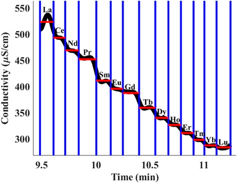
Experimental demonstration of the separation of trivalent lanthanides using plateau-mode ITP. A graph of the measured conductivity signals vs time is shown. The distance between the vertical lines represents the characteristic temporal band length. The mean conductivity signals for each lanthanide are indicated by horizontal lines. The figure was reproduced with permission from ref (359). Copyright 2019 John Wiley and Sons.

11.3. Bioassay Systems That Leverage ITP

11.3.1. DNA and RNA purification and On-Chip Assays

ITP has been extensively used in the development of several DNA- and RNA-based assays over the past decade.^{32,91,92,94,112,202,207,209,379} ITP NA assays are currently the most common applications of microfluidic ITP in biology and biotechnology. Microfluidic ITP applications for NA analyses can be broadly categorized as either those that use ITP for NA purification and preconcentration (i.e., sample prep) prior to downstream analyses (e.g., PCR) or those that combine ITP-based preconcentration or separation with direct on-chip target NA detection. NAs are highly soluble, have a high electrophoretic mobility and a relatively low pK_a of ∼3, and are ideally suited for manipulation and focusing using anionic ITP. These ITP systems are typically buffered near pH 7–9 to ensure that background contaminants (e.g., proteins and downstream inhibitors) from raw biological samples such as blood, urine, and plasma do not focus and interfere with NA-based ITP assays. In all NA-based ITP applications, NAs are typically detected in peak-mode ITP (e.g., using fluorescence), since they are usually present in trace quantities (e.g., nanomolar or lower concentrations) compared to the buffering ions (e.g., millimolar concentration). Further, the free-solution electrophoretic mobilities of DNA and RNA are nearly independent of the length or sequence.³⁸⁰ Hence, all DNA and RNA typically focus into a single concentrated peak in ITP. For fluorescence detection, nucleic acids are typically either synthetically prelabeled (e.g., using fluorescence-tagged oligos) prior to the assay or labeled on-chip using intercalating fluorescent dyes (e.g., SYBR). We refer to Rogacs et al.³¹ for a comprehensive review on the design, development, and applications of ITP systems for nucleic acid purification and sample prep. We also refer to three review articles^38,65,381 that discuss in detail ITP applications for NA-based assays.

The studies of Kondratova et al.³⁸³ and Kondratova et al.⁹² in 2005 were the earliest to report the extraction of DNA from biological samples such as plasma and serum using ITP. They demonstrated their method using fairly standard laboratory equipment (not microfluidics) and agarose gels as a downstream step following a series of purification steps. The study of Schoch et al.¹¹⁰ published in 2009 was likely the first to demonstrate the extraction of nucleic acids using ITP in microfluidic channels. They used ITP and a sieving matrix to selectively extract and preconcentrate small RNAs from the cell lysate (refer also to Han et al.²⁰⁹ for another recent example of simultaneous RNA extraction and size selection using ITP). Subsequently, Persat et al.³² demonstrated the ITP extraction of DNA from whole blood (Figure 31A) and showed the compatibility of the extract with PCR. Thereafter, several ITP systems were developed that combined the ITP extraction of nucleic acids with downstream nucleic acid amplification. For example, Marshall et al.³⁷⁹ used ITP to extract DNA from malaria-containing erythrocyte mixtures and then detected and quantified the extracted pathogenic DNA using off-chip PCR. A similar assay was later integrated on a printed circuit board device (Figure 31B).³⁸² As another example, Borysiak et al.³⁸⁴ used ITP to extract DNA and integrated it with on-chip LAMP amplification to detect Escherichia coli from whole milk. In a similar vein, Eid and Santiago³⁷⁷ combined ITP extraction and downstream recombinase polymerase amplification (RPA) to detect inactivated Listeria monocytogenes from whole blood.

Figure 31.

(A) Purification of genomic DNA from whole blood using ITP. The experimental visualization of the ITP peak containing label DNA (top) and the quantification of the amount of focused DNA (bottom) are shown. The figure was reproduced with permission from ref (32). Copyright 2009 American Chemical Society. (B) Schematic of an ITP assay for cell lysis and nucleic acid extraction implemented on a printed circuit board-based device. Purified DNA was extracted into the LE reservoir and used for off-chip PCR analysis for malaria detection. The figure was reproduced with permission from ref (382). Copyright 2012 American Chemical Society.

More recently similar methods have been implemented on paper-based devices.^236,257,385 A notable example is the work of Bender et al.,²³⁶ who used a paper-based device for the simultaneous ITP extraction of DNA and RPA-based target amplification and demonstrated the detection of HIV-1 DNA from whole blood within clinically relevant viral abundances. As another example, Sullivan et al.³⁸⁵ recently developed a paper-based microfluidic ITP device for extracting nucleic acid from whole blood. Notably, their device integrates whole blood fractionation, plasma protein digestion, and ITP extraction of nucleic acids on a single device. Such portable paper-based devices are likely compatible with point-of-care applications. Research efforts toward rapid point-of-care ITP applications are currently being pursued, with the main goals of reducing intermediate manual steps, the on-chip integration of sample lysis and pre-extraction protocols, improving sensitivity and assay robustness, and minimizing bulky instrumentation.

These studies have demonstrated that ITP is an attractive method for NA purification because of its selectivity to NAs without the use of membranes or toxic chemicals typical of conventional approaches. Besides, ITP provides high yields of NAs regardless of the input sample amount and does not incur losses for small NAs, unlike conventional solid-phase or liquid-phase extractions methods.³¹ Nucleic acid extraction efficiencies of up to 80% have been demonstrated in microfluidic ITP for DNA sample inputs in the range from 250 pg to 250 ng.²³⁰ Using ITP, a similar high efficiency was also demonstrated for input sample amounts as small as the total RNA from a single cell.³⁸⁶ ITP-based NA purification has also been shown to be superior (by over two orders of magnitude) in terms of extraction efficiency compared to commercially available kits for small size nucleic acids (e.g., <60 nt).³⁸⁷

We note that most of the ITP-based NA assays described above require sample lysis (e.g., using Proteinase K, heat, or a surfactant) prior to loading the sample on the chip. It is important that the lysis procedure is compatible with ITP. We refer to ref (31) for a detailed discussion on this topic, including different procedures recommended for RNA versus DNA extraction. Another limitation of ITP is the common requirement to dilute the raw sample (typically between 1:10 and 1:100 in either the TE or the LE) prior to on-chip loading . This is typically required because raw biological samples typically contain overly high salt concentrations (on the order of ∼100 mM strong salts). The ITP processing of such mixtures can lead to strong variations in pH or challenges associated with the separation capacity.

Most of the studies mentioned above used ITP as a sample preparation process prior to downstream target NA detection. However, ITP systems have also been developed to perform direct on-chip target NA detection. A common strategy used in such applications involve ITP-accelerated hybridization reactions between the probe and target NA, which are typically followed by the on-chip separation of excess unreacted species from reacted molecules (e.g., in homogeneous reaction assays; cf. section 11.4) to improve the sensitivity.^95,207 We refer to the discussion in section 11.4 on ITP-based reactions for a detailed review of such ITP systems (see also the review of Eid and Santiago³⁸).

Another mode of application for the direct on-chip detection and quantification of NAs in ITP is the combination of ITP with downstream separations, including various forms of on-chip capillary electrophoresis,^24,30 for example, for the analysis of DNA fragments such as PCR amplicons. For example, Liu et al.³⁸⁸ used transient ITP to preconcentrate PCR amplicons and used coupled capillary gel electrophoresis to separate, quantify, and analyze DNA fragments between ∼70 and ∼1400 bp. Similarly, Bahga et al.²¹¹ used bidirectional ITP to first preconcentrate a 1 kbp dsDNA ladder and then separated fragments using bidirectional ITP-induced zone electrophoresis, all in a single straight channel in solution. A couple other recent examples of direct on-chip target NA detection are the works of Bender et al.²³⁶ mentioned earlier (simultaneous ITP and RPA) and the ITP-CRISPR approach of Ramachandran et al.⁹⁴ (see section 11.4 for more details).

11.3.2. Protein-Based Assays

Like nucleic acids, proteins can also be focused, preconcentrated, and separated in ITP.^{66,203,373,389} There are , however, generally a smaller number of applications involving on-chip (microfluidic) ITP for proteins analyses compared to NA-based systems. This is likely due to the challenges associated with working with proteins, including their sometimes-limited solubility and the fact that they exhibit a wide range of pH- and buffer-dependent electrophoretic mobilities due to their varied isoelectric points (pI) and size. Such variability makes it difficult to develop generally applicable ITP assay designs and chemistries. Despite these challenges, protein-based systems have been developed in both cationic^90,177,256 and anionic^{36,94,200,390} ITP formats depending on the charge of target proteins. Applications of ITP involving proteins can also be broadly categorized as those that extract, preconcentrate, or separate target proteins (e.g., for direct on-chip detection and quantification) of those that use ITP to aid chemical reactions involving proteins (e.g., for immunoassays). We will here only briefly review a few such applications as illustrations. We refer to a recent article by Han and Khnouf⁶⁶ for a detailed review focused on ITP-based protein systems and applications.

Cui et al.³⁶ used anionic ITP to focus, preconcentrate, and separate three fluorescent proteins, namely, green fluorescent protein (GFP), allophycocyanin, and r-phycoerythrin, into distinct zones. Jacroux et al.⁹⁰ used a series of two cationic ITP systems to separate fluorescence-tagged cardiac troponin I (CTnI) from two other proteins, namely r-phycoerythrin and albumin, with similar isoelectric points. This study highlighted that a judicious choice of buffer and separation conditions is required for protein separations in ITP. Other systems for the detection of CTnI were later developed, as presented in refs (89), (188), and (256). Another interesting example is the work of Qu et al.,¹⁷⁷ who developed an ITP system to extract proteins and nucleic acids simultaneously from raw biological samples using bidirectional ITP (cf. section 12). In this system, proteins (e.g., albumin) focused in cationic ITP, while nucleic acids focused in anionic ITP. This method is shown in Figure 32. Briefly, the raw sample is diluted in a mixture containing TE+ and TE– ions and sandwiched between two zones (located on opposite sides), where one of the zones contains LE+ and the other contains LE– (Figure 32). Here, + and – indicate cationic and anionic components, respectively. Upon the application of an electric field, the cationic and anionic ITP shock waves originate from the same TE or sample reservoir and migrate away in opposite directions. We note that this implementation of bidirectional ITP from Qu et al.¹⁷⁷ is very different from the common case of bidirectional ITP where the cationic and anionic ITP shocks interact²¹² (cf. section 12).

Figure 32.

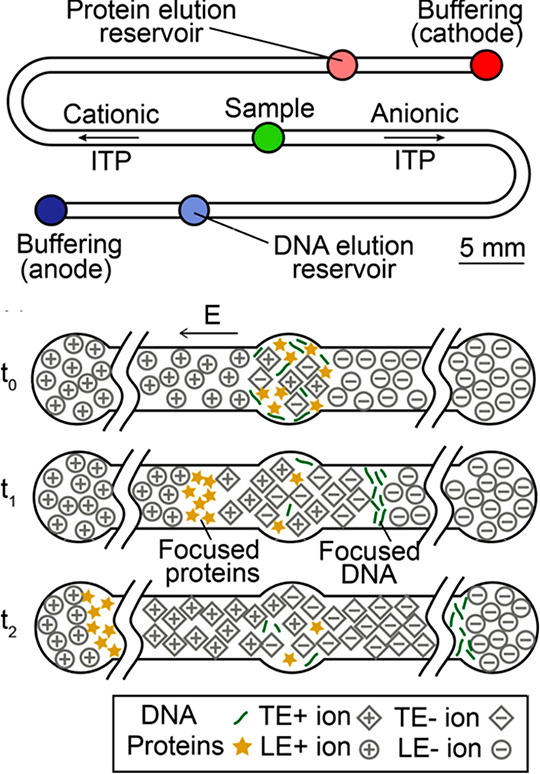
Schematic of an ITP chip (top) and assay (bottom) for the simultaneous extraction of proteins and nucleic acids from raw biological samples through the simultaneous use of noninteracting cationic and anionic ITP, respectively. The cationic and anionic ITP shock waves start from a common sample reservoir and electromigrate in opposite directions to the cathode and the anode, respectively. The figure was reproduced with permission from ref (177). Copyright 2014 American Chemical Society.

Proteins analyses have also been performed by combining microfluidic transient ITP with zone or gel electrophoresis and mass spectrometry. Such systems have been developed, for example, for the analyses of functional proteins in infant milk,³⁹¹ urinary proteins,³⁹² and several other trace-protein analyses.^393,394 Immunoassays that use simultaneous ITP preconcentration and reaction acceleration have also been developed in various formats, including the bead-based assay,^202,389 paper-based lateral flow devices,^255,256 chips with antibody surface functionalization,³⁸⁹ and devices with integrated biosensors that contain binding aptamers³⁹⁰ (cf. Figure 33A). We review in detail several such homogeneous and heterogeneous reaction-based ITP assays for proteins in section 11.4. Lastly, we note that several techniques can be used to “modify” the mobilities of proteins to enable their focusing in ITP. Examples include complexing the protein of interest with specialized aptamers²⁰⁰ (cf. Figure 33B), nucleic acids,⁹⁴ or antibodies²⁵⁶ prior to ITP. Co-focusing proteins and nucleic acids in ITP can also aid NA-based assays (for e.g., RPA and CRISPR),^94,236 which rely on the enzymatic action of proteins on DNA and RNA.

Figure 33.

(A) Schematic illustration of the porous silicon biosensor for ITP-based protein detection. Target proteins are focused in ITP and bind to the aptamers immobilized on a PSiO₂ biosensor. Raw fluorescence images of target protein focusing in peak-mode ITP under pass-over and counterflow operational modes are shown on the right. The figure was reproduced with permission from ref (390). Copyright 2017 American Chemical Society. (B) Schematic of the ITP–spacer assay of Eid et al.²⁰⁰ Initially at t₁, SOMAmers and the target protein are mixed with the LE buffer, and spacer ions are mixed with the TE buffer. Then, at t₂, SOMAmers and the target proteins bind to form low-mobility complexes that electromigrate but are outpaced by spacer ions. At t₃, unreacted SOMAmer molecules focus between the LE and spacer, whereas SOMAmer–target complexes focus between the spacer and the TE. The figure was reproduced with permission from ref (200). Copyright 2015 American Chemical Society.

11.3.3. Single-Cell Analyses

Single cell analyses have gained significant interest over the past few years, since they help explain heterogeneity in cell populations and uncover gene-level interactions between subcellular components. To this end, various microfluidic ITP systems have been developed to study RNA and DNA at the level of single cells, including subcellular components. In 2014, Shintaku et al.⁶³ first developed a microfluidic ITP system that enabled the selective lysing of single living cells, followed by the ITP extraction and quantification of cytoplasmic RNA and its physical separation from the DNA-containing nucleus. In this method, a brief biphasic electric pulse was first used to selectively lyse the outer cell membrane while keeping the nuclear membrane intact. ITP was then used to selectively focus the cytoplasmic RNA (sans the intact nucleus). On-chip fluorescence measurements were used to quantify the heterogeneity in the amounts of DNA and RNA among single lymphocyte cells from the same mouse. Soon thereafter, Kuriyama et al.^386,395 extended the method of Shintaku et al.⁶³ and developed an integrated microfluidic ITP system for the fractionation and recovery of the nucleus and cytoplasmic RNA from single cells (Figure 34). Electric fields (for lysis and ITP) were used to automatically extract cytoplasmic RNA and the nucleus from the same cell at two different channel reservoirs. Downstream RT-qPCR and qPCR were used to quantify cytoplasmic RNA and genomic DNA, respectively. Abdelmoez et al.³⁹⁶ later found that the distinct focusing kinetics observed during ITP-based NA extraction from single cells could be used to distinguish soluble RNA molecules from mitochondrial RNA.

Figure 34.

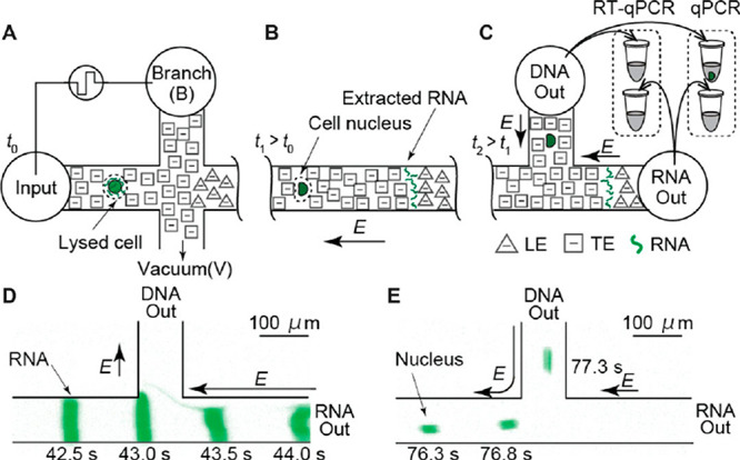
Schematic illustration of the single-cell microfluidic assay of Kuriyama et al.³⁸⁶ (A) A short b-phasic electric pulse is used to selectively lyse the outer membrane of the cell. (B) ITP is used to focus and preconcentrate nucleic acids from the cytoplasm. The nucleus does not focus in ITP but instead electromigrates in the same direction as the ITP peak. (C) Automated electric field control was used to collect the cytoplasmic nucleic acids and nucleus into separate reservoirs. (D and E) Experimental visualizations of the fractionation process shown in panel C. The figure was reproduced with permission from ref (386). Copyright 2015 John Wiley and Sons.

In 2018, Abdelmoez et al.³⁹⁷ significantly expanded the aforementioned ITP-based single-cell approaches and studied correlations of gene expression between nuclear and cytoplasmic RNA (using off-chip RNA sequencing). Their chip included an automated protocol to capture single cells using an integrated hydrodynamic trap. This study was also the first to integrate ITP-based systems with downstream genomic sequencing technologies. The ITP-integrated sequencing approach presented in Abdelmoez et al.³⁹⁷ was termed SINC-Seq.³⁹⁷ A very recent work by Oguchi et al.³⁹⁸ integrated SINC-Seq with nanopore sequencing and studied mRNA isoform diversity within the nucleus and the cytoplasm. As more applications continue to emerge, it is important to keep in mind that current ITP systems for single-cell analyses are limited in throughput (typically limited to one cell per chip/channel) compared to several other high-throughput single cell systems, for example, those based on droplets.^399,400

11.4. Applications of ITP for Accelerating Chemical Reactions

11.4.1. Applications of Homogeneous Reactions Using ITP

In 2008, Kawabata et al.⁴⁰¹ first demonstrated the use of on-chip ITP to control chemical reactions. They used ITP to effect an immunoassay reaction to measure the amount of α-fetoprotein (AFP), a liver cancer marker in blood. ITP was used to focus and preconcentrate a DNA-coupled anti-AFP antibody prior to its reaction with AFP (which did not focus in ITP) in an adjacent zone on chip. The coupling of DNA with the antibody increased the mobility of the DNA–antibody complex and thus enabled it to focus in ITP. Kawabata et al.⁴⁰¹ used on-chip capillary gel electrophoresis (CGE) to separate reaction products and quantify the amount of AFP using LIF. They demonstrated a 140-fold increase in signal due to the ITP format and a detection sensitivity of 5 pM AFP in 136 s. Kawabata et al.⁴⁰¹ called their assay the electrokinetic analyte transport assay (EATA), which involved a homogeneous reaction where only one of the two reactants was focused and preconcentrated in ITP. Such reactions were later modeled by Eid et al.²⁰⁰ Later, Park et al.⁴⁰² presented a method to improve the sensitivity and reproducibility of the EATA assay, and Kagebayashi et al.⁴⁰³ developed a fully automated microfluidic platform that integrated the EATA assay.

Nucleic acids have approximately size-independent and high-magnitude mobilities and are thus attractive for ITP applications. Thus, most of the existing applications of ITP for accelerating biochemical reactions also involved some form of nucleic acid hybridization reactions, including both DNA and RNA. Such reactions involve the reaction between single-stranded nucleic acids and their complementary nucleic acid strand. Goet et al.⁴⁰⁴ first demonstrated that ITP could be utilized to control and bring together two samples and focus them in ITP to initiate chemical reactions. They suggested and qualitatively showed this approach for DNA hybridization reactions. Persat and Santiago¹¹² first applied ITP to initiate, control, and perform hybridization reactions between nucleic acids that were cofocused in ITP. In their study, Persat and Santiago¹¹² showed experiments to quantify hybridization reactions between microRNA (miRNA) and molecular beacons (functionalized with a fluorophore–quencher pair), both of which cofocused in peak-mode ITP (Figure 35). Using this approach, they demonstrated miRNA detection with a 10 pM sensitivity and showed that the ITP reaction was also specific. Subsequently, Bercovici et al.⁴⁰⁵ presented an assay for the detection of bacterial urinary tract infections using ITP-enhanced homogeneous hybridization reactions between bacterial 16S rRNA and complementary molecular beacons. This study integrated the sample purification of urine samples and demonstrated a sensitivity of 100 pM pathogenic target RNA. Later, Bercovici et al.³⁹ developed a comprehensive model for ITP-enhanced second-order homogeneous reactions (cf. section 7.1) and experimentally demonstrated that ITP could accelerate nucleic acid hybridization reactions ∼14 000 fold. The latter was the first study to quantitatively demonstrate the degree of reaction acceleration attributable specifically to the effects of ITP.

Figure 35.

Schematic depiction the ITP hybridization assay of Persat et al.¹¹² (A) The three-stage ITP strategy used for purification and hybridization. LE1 allows for the strong preconcentration of small RNA. LE2 contains a higher polymer concentration to selectively focus miRNA. LE3 allows for specific hybridization. (b) Schematic of the molecular beacon (MB)-based hybridization reaction in ITP. MBs are loaded in the LE, and miRNA is loaded in the TE. They co-focus, preconcentrate, and react in ITP. (C) The reaction of target miRNA with probe MBs results in sequence-specific increase in the fluorescence of the ITP peak. The figure was reproduced with permission from ref (112). Copyright 2011 American Chemical Society.

The aforementioned studies of nucleic acid hybridization utilized molecular beacon reporters to detect a fluorescence signal upon reaction. In their native unreacted state, these reporters have a hairpin structure with quenched fluorescence; this structure disrupted upon hybridization, increasing the fluorescence. An important limitation of such strategies is the finite fluorescence signal of the quenched state, which limits the dynamic range of the signal increase (typically less than two orders of magnitude).

A few studies have addressed the aforementioned limitation of quenched reporters by effecting physical separations of reacted and unreacted species after ITP focusing. Bahga et al.⁴⁰⁶ integrated ITP-enhanced DNA hybridization and capillary zone electrophoresis in-solution using a novel bidirectional ITP scheme. In their approach, anionic ITP was used to speed up the DNA hybridization reaction of the target with a complementary molecular beacon. After a sufficient reaction time, the anionic ITP front interacted with a counter-migrating cationic ITP front, which disrupted the ITP peak and initiated zone electrophoresis that separated the hybrid products from the unreacted beacons. They demonstrated a 5 pM detection sensitivity and an assay time of 3 min and showed that the approach could be used to detect multiple-length ssDNA targets. A limitation of the bidirectional ITP approach is the complexity of buffer design to effect efficient focusing and separation. See Bahga et al.²¹¹ for detailed principles of bidirectional ITP and procedures to choose appropriate buffers. Later, Garcia-Schwarz and Santiago^206,207 developed an alternate strategy wherein the unreacted molecular beacons were captured (and removed from a moving ITP zone) after the reaction using photopatterned, DNA-functionalized hydrogels. In their multistage assay, Garcia-Schwarz and Santiago^206,207 used ITP to first enable a rapid reaction between miRNA and molecular beacons in solution, which was followed by an on-chip separation stage. In the separation stage, the ITP peak migrated into a region of the hydrogel functionalized with probe molecules to capture unreacted beacons. Note that the latter separation stage used a heterogeneous reaction involving immobilized capture probes in the hydrogel, and we will discuss such heterogeneous reactions in the next subsection. The ITP peak that migrated beyond the functionalized hydrogel region consisted only of the hybrid product (i.e., was devoid of unreacted molecular beacons) and was used for detection. Their assay achieved a ∼1 pM detection limit and exhibited a four orders of magnitude dynamic range in detection. Eid et al.⁹⁵ developed another multistage strategy to separate reaction products from unreacted molecules on-chip using ionic spacers and a sieving matrix (Figure 36). In their assay, the spacer ion had a mobility between those of the LE and the TE and formed a plateau between the LE and TE zones in ITP. The reactants focused in peak-mode ITP in solution between the spacer ion an the d LE zone during the first stage of their assay. After the reaction, the ITP peak (and spacer zone) migrated into a region with a sieving matrix (Eid et al.⁹⁵ used 1.8% hydroxyethyl cellulose, HEC, although polyvinylpyrrolidone is another choice¹¹²), where the spacer ion migrated faster than the reaction products but slower than the unreacted probes, thus effecting separation. After a sufficient separation time (∼40 s), the reaction products and unreacted species were refocused among the two ITP interfaces, followed by detection (Figure 36). Using this approach, Eid et al.⁹⁵ obtained a 220 fM ssDNA target detection sensitivity in 10 min and a ∼3.5 orders of magnitude dynamic range. The sieving matrix approach of Eid et al.⁹⁵ requires a well-tailored choice of the sieving matrix and spacer ions depending on the application, which can limit its applicability.

Figure 36.

Schematic of the ITP–spacer assay of Eid et al.⁹⁵ Their assay included three on-chip stages: (1) The reaction between the probe and the target DNA in peak-mode ITP in free solution. In this step, spacer ions electromigrate slower than DNA. (2) The ITP peak electromigrates into a 1.8% HEC sieving matrix region where the spacer molecules outpace the target molecules and probe–target hybrids. (3) The reaction products are fully separated from the unreacted probe, and the molecules are refocused among the two ITP interfaces. The figure was reproduced with permission from ref (95). Copyright 2013 The Royal Society of Chemistry.

A more recent single-step approach to eliminating free probes in ITP-aided reaction assays involves the use of synthetic nucleic acid analogues with weakly charged backbones, such as peptide nucleic acid (PNA) or morpholino, as reaction probes. Assays that rely on PNA and morpholino probes make use of the significantly lower electrophoretic mobilities of probes in solution compared to the higher mobility of the probe-target hybrid. In such assays, a significant excess of probes is typically mixed with the target ssDNA in the TE reservoir to enable rapid target–probe binding prior to the application of electric field. Furthermore, a TE ion is chosen so as to focus only probes that hybridize to the target focus. Ostromohov et al.⁴⁰⁷ utilized PNA probes and an ITP-based “focus upon hybridization” approach and demonstrated a ssDNA detection sensitivity of 100 fM with a dynamic range of five orders of magnitude. See Ostromohov et al.⁴⁰⁷ for the model and theory associated with the approach. Morpholino probes are more soluble than PNA,⁴⁰⁸ which reduces the adsorbance to surfaces and enables the design of longer probe sequences (for example, Ostromohov et al.⁴⁰⁷ used 14 nt PNA probes, whereas Rosenfeld and Bercovici⁹⁹ used 25 nt morpholino probes). Zeidman-Kalman et al.²⁰¹ demonstrated a similar assay based on morpholino probes and used it to develop a method to measure the dissociation kinetics of hybridization. Later, Rosenfeld and Bercovici⁹⁹ implemented an assay based on Morpholino probes in a microfluidic paper-based analytical device (μPAD) to detect ssDNA with a sensitivity of 5 pM in 10 min. The “focus upon hybridization” approach has advantages over excess probe elimination using gel separation or a sieving matrix, as it is a single-step assay and uses simple buffer chemistry.

Unlike DNA and RNA, proteins are large molecules with low mobilities and highly variable ionic charges in solution (due to a wide range of isoelectric points). Electrophoretic mobility depends on the local pH, the ionic strength, and the temperature. For this reason, designing ITP-aided reactions that involve protein focusing is typically more difficult than designing those for nucleic acids. Eid et al.²⁰⁰ presented an ITP assay where modified aptamers called SOMAmers (slow off-rate modified aptamer) were used to bind to typically nonfocusing C-reactive protein (CRP) and enable its focusing and preconcentration in ITP. In this assay, only SOMAmers focused in ITP; native CRP did not focus in ITP but instead remained as a background ion in the LE. As the focused ITP peak swept past the LE, CRP reacted with the preconcentrated SOMAmers and was recruited into the ITP peak. Similar to Eid et al.,⁹⁵ Eid et al.²⁰⁰ used a multistage assay with an ionic spacer and a sieving matrix to separate unreacted SOMAmers from the SOMAmer–protein complex prior to detection to improve the sensitivity. More recently, Ramachandran et al.⁹⁴ demonstrated the use of ITP to control and enhance a reaction involving clustered regularly interspaced short palindromic repeats (CRISPR)-associated enzyme, Cas12 (Figure 37). They showed that the complex comprised of the enzyme and target-specific RNA (guide RNA or gRNA) cofocused in ITP along with free nucleic acids. In their assay, the CRISPR–gRNA first recognized the target nucleic acid via sequence complementarity, then the CRISPR enzyme became activated and cleaved reporter molecules, which released fluorescence. The cofocusing of the CRISPR–gRNA complex together with target and reporter nucleic acids accelerated enzymatic activity and enabled them to develop a rapid, 35 min assay to detect the RNA of SARS-CoV-2 (the virus that causes COVID-19). The ITP-controlled, CRISPR enzyme reaction process in this assay was completed in 5 min. Unlike the assay of Eid et al.,²⁰⁰ the CRISPR assay of Ramachandran et al.⁹⁴ involved the ITP preconcentration and focusing of all reactants, including protein enzymes and nucleic acids.

Figure 37.

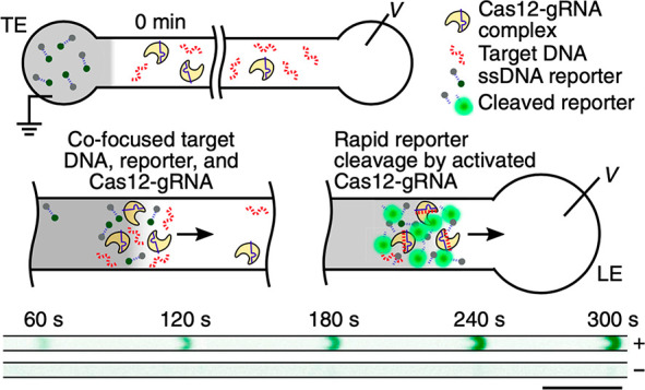
ITP–CRISPR enzymatic assay from Ramachandran et al.⁹⁴ for nucleic acid detection. ITP co-focuses the CRISPR–Cas12–gRNA complex along with the target and reporter nucleic acids. Recognition of the target DNA by the enzyme complex activates the enzyme. Upon activation, the enzyme cleaves ssDNA reporter molecules, resulting in an increase in the fluorescence signal of the ITP peak. The scale bar represents 0.5 mm. The figure was reproduced with permission from ref (94). Copyright 2020 National Academy of Sciences.

11.4.2. Applications of Heterogeneous Reactions Using ITP

In 2014, Karsenty et al.²⁰² first demonstrated the control and enhancement of surface reactions using ITP. They studied nucleic acid hybridization aided by ITP, wherein the target molecules focused in ITP and the probes were immobilized on a surface of the microchannel. The reactive surface was formed within a microchannel by fabricating a trench on one of the channel wall, then prefilling the trench with probe-functionalized paramagnetic beads and immobilizing them. The nucleic acid probes were biotinylated and bound to streptavidin-coated magnetic beads prior to on-chip loading. As the ITP peak passed over the reaction surfaces, fluorescence-labeled target molecules from the ITP peak reacted with surface probes, and the probe–target hybrids were immobilized on the beads, enabling detection. A limitation of this simple pass-over approach (cf. section 7.2) of Karsenty et al.²⁰² is the short incubation time of the target molecules in ITP with surface probes for reaction; this value is limited by the finite residence time of the ITP zone. Despite this, Karsenty et al.²⁰² demonstrated ∼100-fold improvements in the signal and LOD for a 3 min assay compared to standard flow-through assay.

Also in 2014, Han et al.²⁰⁴ demonstrated that ITP could be used to improve the speed and sensitivity of traditional microarray-based assays involving nucleic acid hybridization (Figure 38). Notably, Han et al.²⁰⁴ were the first study to demonstrate multiplexed DNA hybridization reactions using ITP. The study involved reactions between 20 probe and target pairs across 60 microarray spots, with the probes immobilized on the spots and the targets focused in ITP. They developed an operation scheme where a high electric field was applied to rapidly focus nucleic acids, then turned off to allow the ITP peak to diffuse and homogenize within a narrow channel cross-section. ITP focusing and electromigration was then reinitiated at a slower migration velocity over the microarray spots for efficient hybridization. They demonstrated a 30-fold decrease in assay time compared to conventional 15 h microarray assays and simultaneously improved the sensitivity by an order of magnitude without sacrificing specificity.

Figure 38.

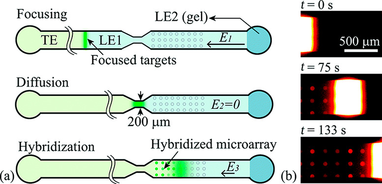
Schematic of the multiplexed microarray heterogeneous reaction system of Han et al.²⁰⁴ (A) ITP is used to focus target DNA in peak-mode ITP. When the ITP peak reaches the constriction, the electric field is briefly turned off to allow the ITP peak to homogenize prior to downstream hybridization. A low electric field is used for the latter hybridization step to maintain a homogeneous ITP peak across the channel width. (B) Experimental images showing the increase in the fluorescence of the microarray spots when the immobilized probes hybridize with fluorescent DNA target molecules. The figure was reproduced with permission from ref (204). Copyright 2014 The Royal Society of Chemistry.

In 2014, Khnouf et al.³⁸⁹ demonstrated a proof-of-concept method for the ITP-based enhancement of the sensitivities of immunoassays involving heterogeneous reactions. They presented two methods that involved the reaction of a target model protein (BSA) with surface-immobilized antibody probes. In the first method, they used antibody-coated magnetic beads that were initially loaded in the LE buffer and then immobilized on chip using an external magnet to create a reactive surface prior to ITP. In the second approach, they directly bound capture antibodies to the surface a PMMA microchannel using a chemical treatment. In both methods, electrokinetic injection was used to introduce a fixed amount of the target protein. The target was focused and preconcentrated in ITP in solution and then reacted with the probes when the ITP zone passed over the reactive surface region. The ITP-based immunoassay achieved a 100-fold preconcentration of the protein and a LOD in the picomolar range.

In 2017, Paratore et al.²⁰³ significantly expanded on the surface-reaction method of Karsenty et al.²⁰² by designing an ITP-based surface immunoassay and demonstrating the detection of enhanced green fluorescent protein. Paratore et al.²⁰³ used paramagnetic streptavidin beads, which were functionalized with biotinylated capture antibodies off-chip (prior to ITP) and then immobilized within a trench in the microchannel. Notably, this study explored the use of counterflow ITP (CF mode; cf. section 8.2) and the stop-and-diffuse mode (SD mode; cf. section 8.2) to enhance the reaction efficiency. The SD mode is advantageous for low-diffusivity target molecules and a high-viscosity medium. The SD mode provided a 10-fold better LOD of 300 fM compared to that of the simple PO mode (LOD of 3 pM). The SD mode is a useful approach when the location of the ITP peak is tractable in real-time (e.g., using current or voltage monitoring or optical methods). The CF mode performed better than the SD mode and lowered the LOD to 220 fM, but it required a more complicated experimental setup involving accurate flow control. For this reason, the CF mode is recommended only for applications that require extremely low levels of detection. Under optimal assay conditions, Paratore et al.²⁰³ demonstrated a 1300-fold improvement in the LOD compared to that of a standard immunoassay in 6 min. The study further noted that the sensitivity of the ITP-based immunoassay is strongly influenced by the pH and salt concentration, factors that require careful optimization depending on the protein target.

We next review applications involving an ITP-focused reactant and an immobilized reactant in a gel or porous column. Garcia-Schwarz et al.²⁰⁶ first demonstrated volumetric heterogeneous reactions in ITP. In their multistage assay for miRNA detection, Garcia-Schwarz et al.²⁰⁶ first performed homogeneous ITP reaction between target miRNA and (excess) complementary molecular beacons. In the next stage of their assay, excess unreacted beacons were removed from ITP prior to detection using an in-line capture region that consisted of a hydrogel functionalized with capture probes complementary to the reporters. This approach decreased the background signal from molecular beacons in ITP and improved the assay sensitivity. Later, Garcia-Schwarz et al.²⁰⁷ adopted this approach and developed a highly specific ITP assay with single-nucleotide specificity for miRNA detection. In particular, they demonstrated the enrichment and specific detection of let-7a miRNA from a mixture of eight miRNAs of the let-7 miRNA family, which differed by a single to a few nucleotides. Their 15 min assay was 1000-fold more sensitive than Northern Blotting and 10-fold faster than RT-PCR.

Another application of ITP to enhance a volumetric heterogeneous reaction is the work of Shkolnikov and Santiago.^205,409 They developed a method that coupled in-line ITP and affinity chromatography (AC) and applied it to the detection and separation of sequence-specific nucleic acids. The affinity substrate was poly(glycidyl methacrylate-co-ethylene dimethacrylate) porous polymer monolith (GMA-EDMA PPM), which allowed for the easy immobilization of affinity probes. Moreover, the affinity column had negligible nonspecific binding and, unlike gels, the affinity column was nonsieving. Shkolnikov and Santiago^205,409 used ITP to first preconcentrate all nucleic acids from the sample in free solution. The ITP peak then electromigrated to the affinity-based column region to capture target DNA molecules. They demonstrated the capture of target DNA from a 10 000-fold higher abundance of background DNA, starting from 200 μL of the sample in a column with a length less than 1 mm in <10 min. They also developed and experimentally validated a model to predict the spatiotemporal behavior of the coupled ITP and AC process, including figures of merit such as the capture efficiency and the capture length.

ITP has also been implemented on paper-based microfluidic devices to improve the sensitivity of lateral flow assays (LFA). Moghadam et al.²⁵⁴ demonstrated ITP sample extraction on a nitrocellulose-based paper microfluidic device and showed that ITP could preconcentrate sample by 900-fold, achieving about a 60% sample recovery efficiency. Later, Moghadam et al.²⁵⁵ integrated ITP extraction in a later-flow immunoassay format and demonstrated both fluorescent (using AF488 dye) and colorimetric (using gold nanoparticles) readouts. IgG secondary antibodies were used as the target and capture reagents. ITP was used to focus target analytes into a thin band and transport them via electromigration to the LFA capture line. The preconcentration of the target prior to the reaction with the capture probes on the LFA capture line dramatically increased the reaction rate associated with the slow reaction kinetics of surface binding in LFA (Figure 39). They demonstrated a 400-fold improvement in the LOD for a 90 s assay time compare to conventional LFA. They estimated the gain factor in the LOD in terms of the fraction of bound probe in ITP-LFA versus conventional LFA formats scales as pk_offt_ITP. Here, p is the effective focusing ratio, k_off is the reaction off-rate, and t_ITP is the ITP residence time. Importantly, they found that the LOD gain factor due to ITP is independent of the dissociation constant, K_D. The gain can be tuned by controlling applied current, which in turn governs the focusing ratio and the ITP residence time. In a similar approach, Guo et al.⁴¹⁰ devised a novel approach to alter the electrophoretic mobility of proteins by immunobinding the target proteins to primary and secondary antibodies and showed that BSA (negatively charged protein) focused in cationic ITP in a fiberglass paper-based microfluidic device. Guo et al.²⁵⁶ expanded on the work of Guo et al.⁴¹⁰ and developed an ITP-LFA assay for the simultaneous detection of two cardiac makers (cTnT and cTnI) from human serum. Similar to Moghadam et al.,²⁵⁵ Guo et al.²⁵⁶ utilized ITP (specifically cationic ITP) to preconcentrate target cardiac protein markers prior to the LFA capture line and to enhance the reaction of the target with monoclonal antibody (mAb) probes on the LFA capture line.

Figure 39.

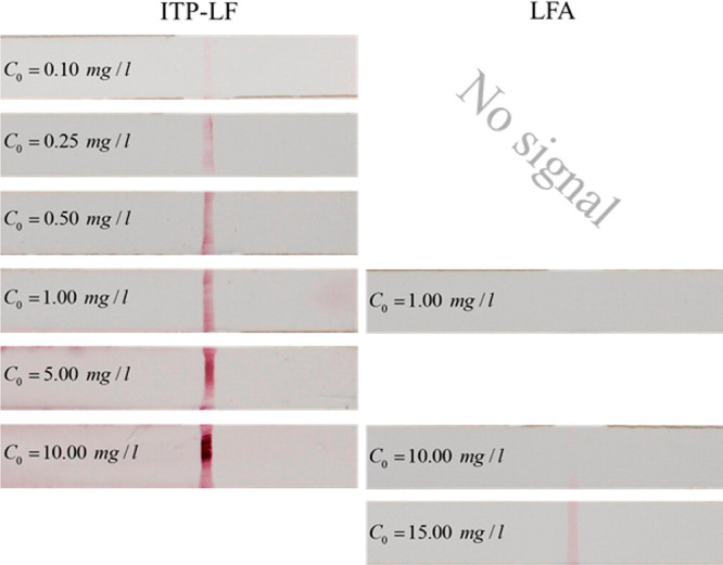
Improvement in the sensitivity of lateral flow assays with ITP. Qualitative estimation of the LOD of an ITP-enhanced assay vs a conventional lateral flow assay (LFA). Here, goat antimouse IgG labeled with 40 nm colloidal gold was used as the target, and the assay time was 5 min. Qualitatively, no signal was observed in the conventional LFA for target concentrations below 10 mg/L, whereas the ITP-enhanced assay detected target concentrations as low as 0.1 mg/L. The figure was reproduced with permission from ref (255). Copyright 2015 American Chemical Society.

11.4.3. ITP Reactions Involving Molecules and Particles or Cells

We here discuss ITP reaction assays that involve particles such as cells and functionalized micrometer-sized beads that either focus in peak-mode ITP or are involved in a reaction with focused small molecules. For small particles, the particle number density multiplied by the number of reactive sites per particle can be treated as an effective volumetric concentration affected by ITP focusing. For sufficiently small particle-to-particle distances, we can ignore diffusion to and from particle surfaces and treat the particle-bound reactant in a manner very similar to a dissolved species (this results in a pseudo-homogeneous ITP reaction). If the particle diameter is on the order of or significantly larger than the axial length of the ITP zone, we can treat the particle as a finite immobilized surface.

Goet et al.²²⁴ first demonstrated that micrometer-sized beads can focus in ITP and presented an analysis of focusing conditions. Later, Shintaku et al.²²⁵ developed a multiplexed bead-based assay to speed up nucleic acid hybridization reactions (Figure 40A). In their work, Shintaku et al.²²⁵ used commercially available ∼6.5 μm magnetic beads (Luminex, Austin, TX) functionalized with 10 different ssDNA probe sequences complementary to various targets in the sample. Upon the application of the electric field, both beads and target DNA focused and preconcentrated in peak-mode ITP, enabling the acceleration of the reaction kinetics. They applied moderate-to-high voltages to induce instabilities in the ITP peak to promote the mixing of the beads with the target. The assay was operated in a regime where the probes (via focused beads) were in excess and the rate of product formation was limited by the influx of the target into the ITP peak. They demonstrated a 60-fold reduction in the reaction time due to the bead-based ITP reaction, achieving the same level of sensitivity and specificity as a well-stirred standard reaction.

Figure 40.

Three example ITP systems involving reactions among molecules and particles or cells. (A) Bead-based hybridization assay from Shintaku et al.²²⁵ Beads functionalized with probe DNA co-focus with target nucleic acids in ITP. This co-focusing and preconcentration accelerates the reaction between the probe and the target. The figure was reproduced with permission from ref (225). Copyright 2014 John Wiley and Sons. (B) ITP-based in situ fluorescence hybridization assay of intact bacterial cells from Phung et al.⁴¹¹ Intact cells co-focus and preconcentrate along with 16s RNA probes in ITP. The figure was reproduced with permission from ref (411). Copyright 2017 American Chemical Society. (C) Microfluidic assay for continuous bacteria detection from Schwartz et al.²⁴⁷ The ITP peak, which contains focused antimicrobial peptides, is held stationary using a counterflow, while bacterial cells flow through the channel via pressure-driven flow. As the cells flow though the ITP peak, they are labeled and detected downstream. The figure was reproduced with permission from ref (247). Copyright 2014 American Chemical Society.

Schwartz et al.²⁴⁷ first demonstrated that ITP could be used for the in-line labeling of bacterial cells (Figure 40C). They used a stationary cationic ITP peak (electromigration countered by a pressure-driven flow) to preconcentrate and focus fluorescence-labeled antimicrobial peptides (AMP). Bacterial cells were continuously flowed through the LE, but they did not focus in ITP. As the cells flowed through the ITP peak, they rapidly reacted with the AMPs and were labeled prior to inline downstream quantification. In this case, to achieve efficient labeling, the reaction time scale must be short compared to the advection time scale of the cells across the ITP peak. This provides a physical limit on the maximum electric field and the throughput of the system. The work of Schwartz et al.²⁴⁷ used AMPs that nonspecifically bound to the negatively charged outer membrane of bacteria and thus provided the ability to selectivity detect bacteria. However, the method was not able to distinguish between different bacteria. To overcome this limitation, Phung et al.⁴¹¹ developed a two-stage ITP assay for the in-line fluorescence in situ hybridization (FISH) labeling of bacterial cells (Figure 40B). Specificity in FISH was obtained by designing appropriate FISH probes for target bacterial cells in the sample. The FISH probes and bacterial cells were simultaneously focused into a small volume and reacted in ITP, and a counter-pressure-driven flow was used to increase the hybridization time. Similar to Eid et al.,⁹⁵ unhybridized probes were then separated from cells in-line using a sieving matrix and spacer ion prior to detection. Phung et al.⁴¹¹ compared their ITP-based FISH to off-line standard FISH and reported a decrease in total assay time from 2.5 h to 30 min.

12. Miscellaneous Configurations of Microfluidic ITP

This section briefly reviews miscellaneous configurations used for ITP processes and analyses. Our intent is not to provide an extensive review but instead to present illustrative examples of (and some references for) the wide variety of configurations possible.

12.1. ITP Preconcentration Followed by Electrophoretic Separation

Capillary electrophoresis (CE) typically provides the best separation performance of any electrokinetic separation method.⁴³ This is due to CE’s capability for analyte mobility resolution and peak capacity (the number of separated species in one experiment), among other figures of merit. In the plateau mode, ITP offers some separation capacity. However, compared to CE, ITP’s clear advantage is a superior sensitivity due to its strong capability for, and highly selective, analyte focusing (i.e., increase of the concentration). In the peak mode, ITP also offers the ability to achieve highly focused and spatially resolved peaks containing multiple species. An excellent way to combine the separation power of CE and the focusing capabilities of ITP is to couple ITP preconcentration with subsequent capillary electrophoresis. Bahga and Santiago²⁴ cover in detail methods, configurations, chemistries, advantages, and disadvantages of such couplings. In this section, we review just a couple of these many coupling strategies.

The most common and easiest to implement method to couple ITP and CE (and even mass spectrometry) is t-ITP.⁸⁴Figure 41 shows an example t-ITP chip layout that uses a column-coupled configuration (essentially a T-junction) for coupling ITP with downstream zone electrophoresis.²⁴ In this configuration, the sample is mixed with the TE and placed in the west reservoir, while the rest of channels, including the north and east reservoirs, are filled with the LE. In the first step, an electric field is applied from east to west (i.e., from the LE to TE reservoirs) to focus and preconcentrate the target analytes in (peak- or plateau-mode or a combination thereof) ITP. The second step is initiated once the ITP peak migrates past the T-junction. Here, an electric field is applied from the north to east reservoirs (both of which are LE reservoirs). The latter step introduces LE ions behind the TE ions. LE ions outpace the TE ions, eventually exposing the analytes locally only to LE ions, hence disrupting ITP and commencing capillary zone electrophoresis-type separation. Various other chip designs (including simple straight channels) and loading configurations can be used for t-ITP.²⁴ Recently, changes in temperature have been used to effect t-ITP using thermally responsive gels, which can be used to strongly vary micromolar analyte mobility.⁴¹² t-ITP is likely most effective when preconcentration is achieved in the peak mode. By far the biggest disadvantage of t-ITP is the high degree of electromigration dispersion imparted on the analyte ions as LE ions are used to displace TE ions (or vice versa). This dispersion limits the resolution that can be achieved by CE as it increases the effective injection sample width at the start of CE. We refer to the ref (24) for a detailed review on coupling t-ITP with zone electrophoresis and refs (29), (96), (109), (111), (304), (306), (324), and (413−415) for various applications of t-ITP in microfluidics.

Figure 41.

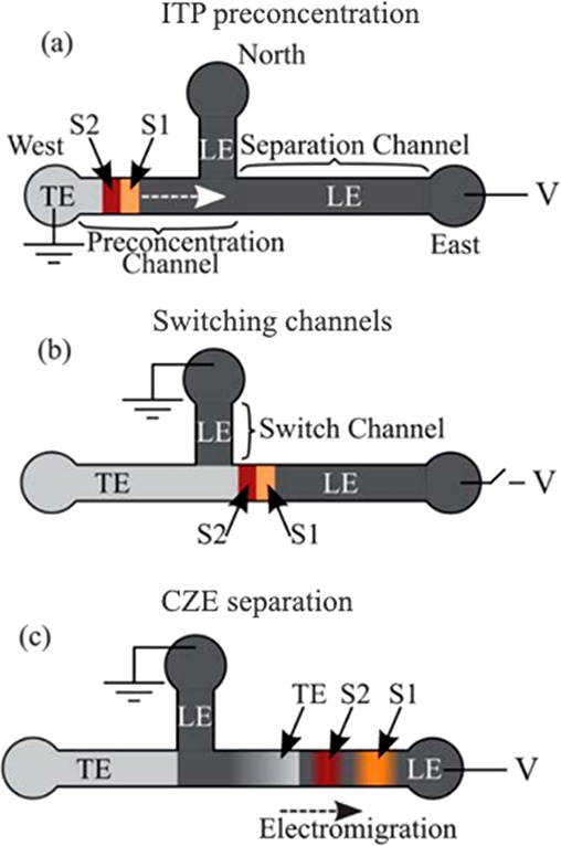
Schematic of an example column-coupling configuration for t-ITP/CZE implemented in a microfluidic chip. The west reservoir is loaded with the TE and the sample, and the remaining channel (including the main channel and the north and east reservoirs) is loaded with the LE. (A) ITP preconcentration of the sample is initiated by the application of an electric field between the east and west reservoirs. (B) As the ITP zone passes the branched section, the applied electric field is switched and applied between the east and north reservoirs. (C) Disruption of ITP and the initiation of CZE separation. The figure was reproduced with permission from ref (24). Copyright 2013 The Royal Society of Chemistry.

Bidirectional ITP offers a way to preserve and leverage the initial high spatial resolution and sample concentration of a peak-mode ITP process while also coupling CE separation. In bidirectional ITP, counter-migrating cationic and anionic ITP processes are established in the same channel. As shown in Figure 42, the cationic and anionic ITP shock waves typically originate in the two end-channel reservoirs and migrate toward each other. This is achieved using two sets of LE and TE ions, namely, cations LE+ and TE+ for cationic ITP and anions LE– and TE– for anionic ITP. LE+ and TE– ions are loaded in the cathodic reservoir, TE+ and LE– ions are loaded in the anodic reservoir, and the main channel is filled with a mixture containing LE+ and LE–. Upon the application of an electric field, the cationic shock wave migrates from the anodic reservoir toward the cathode, and the anionic shock wave migrates from the cathodic reservoir toward the anode. At an intermediate time, these two countermigrating shock waves interact with each other and disrupt the ITP process, resulting in the formation of a new (background) zone composed of TE+ and TE–, wherein analyte ions undergo CE-type separation. This configuration was used by Bahga et al.²¹¹ and Bahga et al.⁴⁰⁶ to preconcentrate and subsequently separate DNA molecules, including a 1 kbp DNA ladder and hybridized DNA products, from unhybridized ssDNA. We refer to refs (416−423) for detailed discussions around theory, simulations, and applications of bidirectional ITP. A disadvantage of the bidirectional ITP method is that the design of assay chemistries can be complex (requiring two sets of carefully chosen and compatible LEs and TEs), which can limit the possible range of analyte mobilities that can be separated.

Figure 42.

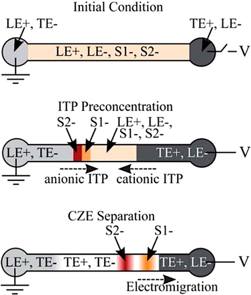
Schematic depicting ITP/CZE achieved using bidirectional ITP in a straight channel. Sample ions focus and preconcentrate in anionic ITP prior to the interaction of the anionic ITP shock wave with a countermigrating cationic ITP shock wave. Upon the interaction of these shock waves, ITP is disrupted and electrophoretic separation is initiated via the formation of a new “background” zone composed of TE⁺ and ^TE– ions. The figure was reproduced with permission from ref (24). Copyright 2013 The Royal Society of Chemistry.

12.2. Cascade ITP

Recall from section 6 that the concentration of plateau zones in ITP scale proportionally with the LE ion concentration. Additionally, the plateau-mode concentration is determined by the LE ion concentration, the LE ion mobility, and the plateau species mobility. Cascade ITP leverages these features using a sequence of LE zones with varied LE ion concentrations to improve the detection sensitivity. In one approach, analytes are initially focused behind one LE zone with a high concentration, enabling strong sample focusing and a high separation capacity. Subsequently, the focused zone electromigrates into a downstream region formerly occupied by a LE with a lower ionic strength. The local electric field is higher in the latter zone, which can be used to raise the concentration of a peak-mode analyte distribution. The approach was first introduced by Boček et al.⁴²³ for capillary ITP systems, who used it to demonstrate the complete separation of ions that typically formed mixed zones in ITP. Cascade ITP was later introduced in microfluidic ITP by Kaniansky et al.²⁵⁰ using a column-coupled configuration to load electrolytes. More recently, Bahga et al.²¹² adapted bidirectional ITP to achieve a cascade of LE concentrations and used it to demonstrated cascade ITP in a single straight channel chip. See also Guo et al.²⁵⁶ for an example of cascade ITP implemented on a paper-based microfluidic device.

12.3. Counterflow and Gradient-Elution ITP

One approach for increasing the processing capacity of an ITP system while minimizing the sample length is to apply the flow of the bulk liquid in a direction opposed to the direction of the ITP. The flow can be achieved using an externally applied pressure gradient⁴²⁴ or the inherent electro-osmotic mobility of the channels.⁴²⁵ In either case, the effect is to enable a longer duration of ITP in a relatively short channel. Figure 43 shows an example implementation of counterflow ITP from the work of Phung et al.⁴²⁶ In step i, the sample is diluted in the TE and loaded in a semi-infinite injection mode. In step ii, a constant pressure-driven flow is applied to approximately balance the electrophoretic motion of the ITP peak. Between steps ii and iii, sample ions continuously focus at the stationary ITP interface. Finally, in step iv, the pressure-driven flow is stopped and the peak is allowed to electromigrate to a detector placed downstream. Phung et al.⁴²⁶ used this setup to detect bacterial cells in ITP and showed that the counterflow improved the LOD by a factor of four compared to the case with no flow. See refs (60), (180), (328), (379), (427), and (428) for various other studies and applications that use counterflow in ITP.

Figure 43.

Schematic of counterflow ITP. In step i, the sample is mixed with the TE, and the mixture is loaded via semi-infinite injection. In step ii, the electric field is applied and ITP is initiated. A counterflow is also applied using a hydrodynamic pressure head to balance the electromigration. In step iii, the sample accumulates in the stationary ITP zone over time. In step iv, the counterflow is turned off, and the ITP peak migrates downstream for detection. The shape of the LE-to-TE interface is idealized, as the pressure-driven flow tends to disperse this interface. The figure was reproduced with permission from Phung et al.⁴²⁶ Copyright 2015 Springer Nature.

Another implementation of counterflow in ITP is so-called gradient elution ITP, first shown by Shackman and Ross.⁴²⁹ In a first step, the effect of the applied electric field and a (dominant) counter-flow (EOF or pressure-driven flow) lead to a configuration where LE anions fill the entire length of a free-standing capillary connected to a reservoir filled with the TE buffer and anionic analyte species, as shown in Figure 44. In this configuration, analyte ions focus at the LE–TE interface near the channel entrance, as indicated in the figure. After sufficient analyte focusing, the counterflow is controlled to permit analyte ions to enter in an order indicative of the effective mobility of the analytes. We know of no quantitative analysis of this process, but the operation is reportedly robust and has been applied to the ITP separation and controlled elution of amino acids and DNA.^430−434 Disadvantages of the technique include a requirement for precise pressure-driven flow control and repeatable and controllable EOF channel mobility.

Figure 44.

Gradien- elution ITP. (a) Schematic of the experimental setup used by Shackman and Ross.⁴²⁹ (b) A combination of EOF and hydrodynamic flow is used to focus and accumulate analyte ions between the LE and TE interface at the entrance of the capillary or channel. After this initial focusing, the counterflow is regulated to control the release of analyte species in to the main channel based on the species mobility values. (c–f) Experimental images showing the controlled injection of carboxyfluorescein (FAM) and fluorescein (F) I to the channel for applied pressures of 1800, 850, 730, and (f) 590 Pa, respectively. (g) Electropherogram showing the separation of F and FAM using gradient-elution ITP. The figure was reproduced with permission from ref (429). Copyright 2007 American Chemical Society.

12.4. Free-Flow ITP

Free-flow ITP is a two-dimensional process that couples bulk flow and ITP electromigration in perpendicular directions. The system configuration is similar to that of so-called free-flow electrophoresis.^245,435,436Figure 45 shows experimental visualizations of free-flow ITP from Janasek et al.²⁴⁵ In the figure, pressure-driven flow is established along the axial direction of a channel (downward) with a relatively shallow depth (into the image) and a relatively large spanwise width (horizontal). Along the left and right spanwise (vertical) edges of the chamber are trenches of TE and LE buffers integrated with linear electrodes, which establish a horizontal electric field directed from right to left. Sample ions introduced at the entrance (top) undergo ITP-type focusing as they flow downward. Free-flow ITP allows for continuous focusing and spatial separation (e.g., if focused to the point of plateau-mode ITP). Refer to Turgeon et al.²⁴⁶ and Novo and Janasek⁴³⁷ for detailed reviews around the theory and applications of microfluidic free-flow ITP.

Figure 45.

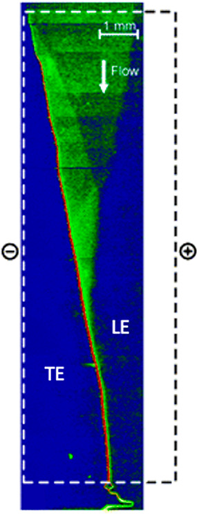
Experimental demonstration of free-flow ITP by Janasek et al.²⁴⁵ A heatmap of the fluorescence intensity in x (horizontal) vs t (vertical) is shown, where red and blue represent the highest and lowest fluorescence intensities, respectively. Here, 5 μM fluorescein was preconcentrated and focused in free-flow ITP under an applied electric field of 525 V/cm. The flow was directed from the top to the bottom at a velocity of 10 μL/min. Figure was adapted with permission from ref (245). Copyright 2006 American Chemical Society.

13. Outlook for ITP in Microfluidics

Microfluidic ITP has been pursued with increased interest and shown significant developments over the last two decades. New applications for the use of ITP in microfluidics continue to emerge, especially in fields of biological science, including molecular biology and diagnostics, chemical analysis, and food and plant sciences. These applications include the use of ITP as both an analytical tool and an intermediate preparatory tool for downstream analyses. We here offer comments around several areas of microfluidic ITP that would benefit from improvements and improved understanding.

Although microfluidic ITP technologies were initially developed (and are easily suited) to handle small sample volumes (typically a few microliters), many emerging technologies, particularly in the field of molecular diagnostics and trace analyte identification, require the processing of large sample volumes—as much as several hundreds of microliters to one or more milliliters—to achieve sufficient sensitivity. To the best of our knowledge, the commercial microfluidic ITP system of Purigen Biosystems, Inc. (IONIC ITP system) currently processes the highest sample input volumes, around 200 μL in under an hour. Key impediments to scaling up ITP channels are Joule heating and the buoyancy effects associated with larger volume systems. The requirement to mitigate Joule heating effects can significantly influence chip and system design and limit the minimum assay time. For example, Joule heating can drive the material, fabrication method, and geometry of system. Buoyancy effects in ITP systems with relatively large cross-sections can arise due to differences in the mass densities of various ITP zones (e.g., the adjusted TE and the LE), which can create an important orientation dependence.

Microfluidic ITP technologies can also strongly benefit from the development of more (or fully) integrated and automated systems and workflows. This is of particular interest for molecular diagnostic systems that seek to provide automated and rapid raw sample-to-answer solutions. One example is nucleic acid detection and identification technologies, including the integration of on-chip sample lysis, ITP-based purification, focusing, mixing, and chemical reactions (such as enzymatic amplification), followed by sensitive on-chip detection (e.g., via fluorescence). Typical challenges associated with such integrated assay systems that use ITP include developing optimized buffer chemistries compatible with the various phases of the assay, optimizing channel designs for ease of use and interfacing various steps, and operation schemes that, in either open- or closed-loop, control and regulate the entire assay. Further, reproducible sample and buffer loading configurations (e.g., that use automatic pressure valves) within the reservoirs and channels are important to ensure the robustness of assays.

Another area for improvement is to better leverage the preconcentration ability of ITP to improve the performance (particularly the sensitivity but also the resolution) of downstream separation systems. As we have discussed, such efforts have been ongoing for decades, but it is the opinion of the current authors that ITP is nevertheless under-utilized as a preconcentration technique prior to separation and identification methods such as capillary electrophoresis, chromatography (including electrochromatography), and mass spectroscopy. In our experience, ITP can often be integrated as a preconcentration method using existing hardware by carefully designing the chemistries and the initial configuration of the sample versus buffers. Another related and emerging research area is the development and integration of hybrid matrix systems for ITP, for example, those involving liquid- and gel-based matrices, including functionalized gels and matrices for specific heterogeneous assay and processing steps (including separations). Such systems should enable new modalities and functionalities.

Lastly, we recommend that easy-to-use modeling and simulation tools be developed (or existing ones expanded) to enable simple assay design and the optimization of buffer chemistries and geometries. Current simulation tools are limited to testing ideas based on ad-hoc user inputs for chemistry and geometry and preclude an easy approach to optimization. We suggest research into the development of “inverse problem” approaches and simulation tools for ITP wherein the user provides target performance requirements and constraints (e.g., estimates of analyte mobilities and pK_a values) as inputs to the simulation and the simulation outputs suggested possible design solutions ranked by performance metrics.

Biographies

Ashwin Ramachandran received his B. Tech in Aerospace Engineering from the Indian Institute of Technology Bombay in 2015 and both his MS and Ph.D. in Aeronautics and Astronautics and his PhD minor in Bioengineering from Stanford University in 2022. His Ph.D. research focused on the modeling and development of electrokinetic microfluidic techniques for biochemical analyses and water desalination. He is currently a postdoctoral scholar at Princeton University in the Departments of Mechanical and Aerospace Engineering and Molecular Biology.

Juan G. Santiago received his Ph.D. in Mechanical Engineering from the University of Illinois at Urbana–Champaign in 1995. He holds the Charles Lee Powell Foundation endowed professorship at Stanford University and is Professor and Vice Chair of the Mechanical Engineering Department. His research includes the development of microsystems for on-chip chemical and biochemical analysis, methods for DNA quantification and analyses, and capacitive deionization. He is a Fellow of the American Physical Society, a Fellow of the American Society of Mechanical Engineering, and a Fellow of the American Institute for Medical and Biological Engineering. He was elected to the American Academy of Arts and Sciences in 2022. He serves and has served on the editorial board of several journals and has cofounded several companies in microfluidics. He is the founding Editor-in-Chief of the Cambridge University Press journal Flow.

Supporting Information Available

The Supporting Information is available free of charge at https://pubs.acs.org/doi/10.1021/acs.chemrev.1c00640.

• Nomenclature of variables and guidelines for buffer design (PDF)

Special Issue

This paper is an additional review for Chem. Rev. 2022, volume 122, issue (7), , “Microfluidics”.

The authors declare no competing financial interest.

References

- Everaerts F. M.; Beckers J. L.; Verheggen T. P. E. M.. Isotachophoresis: Theory, Instrumentation and Applications; Elsevier, 2011. [Google Scholar]
- Boček P.Analytical Isotachophoresis. In Analytical Problems; Topics in Current Chemistry, Vol. 95; Springer, 1981; pp 131–177. [Google Scholar]
- Longsworth L. G.; MacInnes D. A. Electrophoresis of Proteins by the Tiselius Method. Chem. Rev. 1939, 24 (2), 271–287. 10.1021/cr60078a006. [DOI] [Google Scholar]
- Tiselius A. A New Apparatus for Electrophoretic Analysis of Colloidal Mixtures. Trans. Faraday Soc. 1937, 33, 524–531. 10.1039/tf9373300524. [DOI] [Google Scholar]
- Hall J. L. Moving Boundary Electrophoretic Study of Insulin. J. Biol. Chem. 1941, 139 (1), 175–184. 10.1016/S0021-9258(19)51374-6. [DOI] [Google Scholar]
- Gebauer P.; Boćek P. Predicting Peak Symmetry in Capillary Zone Electrophoresis: The Concept of the Peak Shape Diagram. Anal. Chem. 1997, 69 (8), 1557–1563. 10.1021/ac960796d. [DOI] [Google Scholar]
- Gebauer P.; Caslavska J.; Thormann W.; Boček P. Prediction of Zone Patterns in Capillary Zone Electrophoresis with Conductivity Detection: Concept of the Zone Conductivity Diagram. J. Chromatogr. A 1997, 772 (1–2), 63–71. 10.1016/S0021-9673(97)00103-9. [DOI] [Google Scholar]
- Gaš B.; Kenndler E. Dispersive Phenomena in Electromigration Separation Methods. Electrophor. An Int. J. 2000, 21 (18), 3888–3897. . [DOI] [PubMed] [Google Scholar]
- Šustáček V.; Foret F.; Boček P. Selection of the Background Electrolyte Composition with Respect to Electromigration Dispersion and Detection of Weakly Absorbing Substances in Capillary Zone Electrophoresis. J. Chromatogr. A 1991, 545 (2), 239–248. 10.1016/S0021-9673(01)88716-1. [DOI] [Google Scholar]
- Haglund H. Isotachophoresis. Sci. Tools 1970, 17, 2–13. [Google Scholar]
- Everaerts F. M.; Verheggen T. P. E. M. Isotachophoresis. Electrophoretic Analysis in Capillaries. J. Chromatogr. A 1970, 53 (2), 315–328. 10.1016/S0021-9673(01)98471-7. [DOI] [Google Scholar]
- Kendall J.; Crittenden E. D. The Separation of Isotopes. Proc. Natl. Acad. Sci. U. S. A. 1923, 9 (3), 75. 10.1073/pnas.9.3.75. [DOI] [PMC free article] [PubMed] [Google Scholar]
- Longsworth L. G.8. Moving Boundary Separation of Salt Mixtures. In Electrochemical Constants; U.S. Department of Commerce, National Bureau of Standards: Washington, D.C., 1953; p 59. [Google Scholar]
- Ornstein L. Disc Electrophoresis. I., Background and Theory. Ann. N.Y. Acad. Sci. 1964, 121 (2), 321–349. 10.1111/j.1749-6632.1964.tb14207.x. [DOI] [PubMed] [Google Scholar]
- Martin A. J. P.; Everaerts F. M. Displacement Electrophoresis. Anal. Chim. Acta 1967, 38, 233–237. 10.1016/S0003-2670(01)80582-1. [DOI] [PubMed] [Google Scholar]
- Coxon M.; Binder M. J. Isotachophoresis (Displacement Electrophoresis. Transphoresis) Theory: Structure of the Ionic Species Interface. J. Chromatogr. A 1974, 95 (2), 133–145. 10.1016/S0021-9673(00)84072-8. [DOI] [Google Scholar]
- Everaerts F. M.; Verheggen T. P. E. M. Isotachophoresis: Electrophoretic Analysis in Capillaries. J. Chromatogr. A 1970, 53 (2), 315–328. 10.1016/S0021-9673(01)98471-7. [DOI] [Google Scholar]
- Verheggen T. P. E. M.; Mikkers F. E. P.; Everaerts F. M. Isotachophoresis in Narrow-Bore Tubes: Influence of the Diameter of the Separation Compartment. J. Chromatogr. A 1977, 132 (2), 205–215. 10.1016/S0021-9673(00)89293-6. [DOI] [Google Scholar]
- Smejkal P.; Bottenus D.; Breadmore M. C.; Guijt R. M.; Ivory C. F.; Foret F.; Macka M. Microfluidic Isotachophoresis: A Review. Electrophoresis 2013, 34 (11), 1493–1509. 10.1002/elps.201300021. [DOI] [PubMed] [Google Scholar]
- Jorgenson J. W.; Lukacs K. D. Free-Zone Electrophoresis in Glass Capillaries. Clin. Chem. 1981, 27 (9), 1551–1553. 10.1093/clinchem/27.9.1551. [DOI] [PubMed] [Google Scholar]
- Jorgenson J. W.; Lukacs K. D. Capillary Zone Electrophoresis. Science (80-.). 1983, 222, 266–274. 10.1126/science.6623076. [DOI] [PubMed] [Google Scholar]
- Kaniansky D.; Marak J. On-Line Coupling of Capillary Isotachophoresis with Capillary Zone Electrophoresis. J. Chromatogr. A 1990, 498, 191–204. 10.1016/S0021-9673(01)84247-3. [DOI] [Google Scholar]
- Foret F.; Szökő E.; Karger B. L. Trace Analysis of Proteins by Capillary Zone Electrophoresis with On-column Transient Isotachophoretic Preconcentration. Electrophoresis 1993, 14 (1), 417–428. 10.1002/elps.1150140167. [DOI] [PubMed] [Google Scholar]
- Bahga S. S.; Santiago J. G. Coupling Isotachophoresis and Capillary Electrophoresis: A Review and Comparison of Methods. Analyst 2013, 138 (3), 735–754. 10.1039/C2AN36150G. [DOI] [PubMed] [Google Scholar]
- Walker P. A.; Morris M. D.; Burns M. A.; Johnson B. N. Isotachophoretic Separations on a Microchip. Normal Raman Spectroscopy Detection. Anal. Chem. 1998, 70 (18), 3766–3769. 10.1021/ac980195h. [DOI] [PubMed] [Google Scholar]
- Chen L.; Prest J. E.; Fielden P. R.; Goddard N. J.; Manz A.; Day P. J. R. Miniaturised Isotachophoresis Analysis. Lab Chip 2006, 6 (4), 474–487. 10.1039/b515551g. [DOI] [PubMed] [Google Scholar]
- Vreeland W. N.; Williams S. J.; Barron A. E.; Sassi A. P. Tandem Isotachophoresis-Zone Electrophoresis via Base-Mediated Destacking for Increased Detection Sensitivity in Microfluidic Systems. Anal. Chem. 2003, 75 (13), 3059–3065. 10.1021/ac0259921. [DOI] [PubMed] [Google Scholar]
- Zhang B.; Liu H.; Karger B. L.; Foret F. Microfabricated Devices for Capillary Electrophoresis- Electrospray Mass Spectrometry. Anal. Chem. 1999, 71 (15), 3258–3264. 10.1021/ac990090u. [DOI] [PubMed] [Google Scholar]
- Jeong Y.; Choi K.; Kang M. K.; Chun K.; Chung D. S. Transient Isotachophoresis of Highly Saline Samples Using a Microchip. Sensors Actuators B Chem. 2005, 104 (2), 269–275. 10.1016/j.snb.2004.05.011. [DOI] [Google Scholar]
- Wainright A.; Williams S. J.; Ciambrone G.; Xue Q.; Wei J.; Harris D. Sample Pre-Concentration by Isotachophoresis in Microfluidic Devices. J. Chromatogr. A 2002, 979 (1–2), 69–80. 10.1016/S0021-9673(02)01246-3. [DOI] [PubMed] [Google Scholar]
- Rogacs A.; Marshall L. A.; Santiago J. G. Purification of Nucleic Acids Using Isotachophoresis. J. Chromatogr. A 2014, 1335, 105–120. 10.1016/j.chroma.2013.12.027. [DOI] [PubMed] [Google Scholar]
- Persat A.; Marshall L. A.; Santiago J. G. Purification of Nucleic Acids from Whole Blood Using Isotachophoresis. Anal. Chem. 2009, 81 (22), 9507–9511. 10.1021/ac901965v. [DOI] [PubMed] [Google Scholar]
- Chambers R. D.; Santiago J. G. Imaging and Quantification of Isotachophoresis Zones Using Nonfocusing Fluorescent Tracers. Anal. Chem. 2009, 81 (8), 3022–3028. 10.1021/ac802698a. [DOI] [PubMed] [Google Scholar]
- Garcia-Schwarz G.; Rogacs A.; Bahga S. S.; Santiago J. G. On-Chip Isotachophoresis for Separation of Ions and Purification of Nucleic Acids. J. Vis. Exp. 2012, (61), e3890. 10.3791/3890. [DOI] [PMC free article] [PubMed] [Google Scholar]
- Bharadwaj R.; Santiago J. G. Dynamics of Field-Amplified Sample Stacking. J. Fluid Mech. 2005, 543, 57–92. 10.1017/S0022112005005975. [DOI] [Google Scholar]
- Cui H.; Dutta P.; Ivory C. F. Isotachophoresis of Proteins in a Networked Microfluidic Chip: Experiment and 2-D Simulation. Electrophoresis 2007, 28 (7), 1138–1145. 10.1002/elps.200600525. [DOI] [PubMed] [Google Scholar]
- Breadmore M. C.; Kwan H. Y.; Caslavska J.; Thormann W. Dynamic High-resolution Computer Simulation of Electrophoretic Enantiomer Separations with Neutral Cyclodextrins as Chiral Selectors. Electrophoresis 2012, 33 (6), 958–969. 10.1002/elps.201100472. [DOI] [PubMed] [Google Scholar]
- Eid C.; Santiago J. G. Isotachophoresis Applied to Biomolecular Reactions. Lab Chip 2018, 18, 11–26. 10.1039/C7LC00852J. [DOI] [PubMed] [Google Scholar]
- Bercovici M.; Han C. M.; Liao J. C.; Santiago J. G. Rapid Hybridization of Nucleic Acids Using Isotachophoresis. Proc. Natl. Acad. Sci. U. S. A. 2012, 109 (28), 11127–11132. 10.1073/pnas.1205004109. [DOI] [PMC free article] [PubMed] [Google Scholar]
- Svensson H.; Barfod B.; Gjertsen P. The Behaviour of Weak Electrolytes in Moving Boundary Systems I. The Moving Boundary Equation.. ACTA Chem. Scand. 1948, 2, 841–855. 10.3891/acta.chem.scand.02-0841. [DOI] [Google Scholar]
- Dismukes E. B.; Alberty R. A. Weak Electrolyte Moving Boundary Systems Analogous to the Electrophoresis of a Single Protein1. J. Am. Chem. Soc. 1954, 76 (1), 191–197. 10.1021/ja01630a050. [DOI] [Google Scholar]
- Křivaánková L.; Gebauer P.; Boček P.. Isotachophoresis. In High Resolution Separation and Analysis of Biological Macromolecules Part A: Fundamentals; Karger B. L., Hancock W. S., Eds.; Methods in Enzymology, Vol. 270; Academic Press, 1996; pp 375–401. [DOI] [PubMed] [Google Scholar]
- Handbook of Capillary and Microchip Electrophoresis and Associated Microtechniques; Landers J. P., Ed.; CRC Press: Boca Raton, FL, 2007. [Google Scholar]
- Breadmore M. C.; Dawod M.; Quirino J. P. Recent Advances in Enhancing the Sensitivity of Electrophoresis and Electrochromatography in Capillaries and Microchips (2008–2010). Electrophoresis 2011, 32 (1), 127–148. 10.1002/elps.201000412. [DOI] [PubMed] [Google Scholar]
- Kašička V. Recent Developments in CE and CEC of Peptides (2009–2011). Electrophoresis 2012, 33 (1), 48–73. 10.1002/elps.201100419. [DOI] [PubMed] [Google Scholar]
- Kitagawa F.; Kawai T.; Sueyoshi K.; Otsuka K. Recent Progress of On-Line Sample Preconcentration Techniques in Microchip Electrophoresis. Anal. Sci. 2012, 28 (2), 85. 10.2116/analsci.28.85. [DOI] [PubMed] [Google Scholar]
- Wen Y.; Li J.; Ma J.; Chen L. Recent Advances in Enrichment Techniques for Trace Analysis in Capillary Electrophoresis. Electrophoresis 2012, 33 (19–20), 2933–2952. 10.1002/elps.201200240. [DOI] [PubMed] [Google Scholar]
- Breadmore M. C. Recent Advances in Enhancing the Sensitivity of Electrophoresis and Electrochromatography in Capillaries and Microchips. Electrophoresis 2007, 28 (1–2), 254–281. 10.1002/elps.200600463. [DOI] [PubMed] [Google Scholar]
- Gebauer P.; Boček P. Recent Progress in Capillary Isotachophoresis. Electrophoresis 2002, 23 (22–23), 3858–3864. 10.1002/elps.200290006. [DOI] [PubMed] [Google Scholar]
- Gebauer P.; Malá Z.; Boček P. Recent Progress in Capillary ITP. Electrophoresis 2007, 28 (1–2), 26–32. 10.1002/elps.200600396. [DOI] [PubMed] [Google Scholar]
- Gebauer P.; Boček P. Recent Progress in Capillary Isotachophoresis. Electrophor. An Int. J. 2000, 21 (18), 3898–3904. . [DOI] [PubMed] [Google Scholar]
- Malá Z.; Gebauer P. Recent Progress in Analytical Capillary Isotachophoresis. Electrophoresis 2019, 40 (1), 55–64. 10.1002/elps.201800239. [DOI] [PubMed] [Google Scholar]
- Malá Z.; Gebauer P.; Boček P. Recent Progress in Analytical Capillary Isotachophoresis. Electrophoresis 2013, 34 (1), 19–28. 10.1002/elps.201200323. [DOI] [PubMed] [Google Scholar]
- Malá Z.; Gebauer P.; Boček P. Recent Progress in Analytical Capillary Isotachophoresis. Electrophoresis 2015, 36, 2. 10.1002/elps.201400337. [DOI] [PubMed] [Google Scholar]
- Gebauer P.; Malá Z.; Boček P. Recent Progress in Analytical Capillary Isotachophoresis. Electrophoresis 2011, 32 (1), 83–89. 10.1002/elps.201000304. [DOI] [PubMed] [Google Scholar]
- Gebauer P.; Boček P. Recent Application and Developments of Capillary Isotachophoresis. Electrophoresis 1997, 18 (12–13), 2154–2161. 10.1002/elps.1150181206. [DOI] [PubMed] [Google Scholar]
- Bocek P.; Gebauer P.; Dolnik V.; Foret F. Recent Developments in Isotachophoresis. J. Chromatogr. 1985, 334 (2), 157–195. 10.1016/S0021-9673(00)80270-8. [DOI] [PubMed] [Google Scholar]
- Malá Z.; Gebauer P.; Boček P. Analytical Capillary Isotachophoresis after 50 Years of Development: Recent Progress 2014–2016. Electrophoresis 2017, 38 (1), 9–19. 10.1002/elps.201600289. [DOI] [PubMed] [Google Scholar]
- Rubin S.; Schwartz O.; Bercovici M. Sample Distribution in Peak Mode Isotachophoresis. Phys. Fluids 2014, 26 (1), 012001. 10.1063/1.4861399. [DOI] [Google Scholar]
- GanOr N.; Rubin S.; Bercovici M. Diffusion Dependent Focusing Regimes in Peak Mode Counterflow Isotachophoresis. Phys. Fluids 2015, 27 (7), 072003. 10.1063/1.4927230. [DOI] [Google Scholar]
- Garcia-Schwarz G.; Bercovici M.; Marshall L. A.; Santiago J. G. Sample Dispersion in Isotachophoresis. J. Fluid Mech. 2011, 679, 455–475. 10.1017/jfm.2011.139. [DOI] [Google Scholar]
- Bhattacharyya S.; Gopmandal P. P.; Baier T.; Hardt S. Sample Dispersion in Isotachophoresis with Poiseuille Counterflow. Phys. Fluids 2013, 25 (2), 022001. 10.1063/1.4789967. [DOI] [Google Scholar]
- Shintaku H.; Nishikii H.; Marshall L. A.; Kotera H.; Santiago J. G. On-Chip Separation and Analysis of RNA and DNA from Single Cells. Anal. Chem. 2014, 86 (4), 1953–1957. 10.1021/ac4040218. [DOI] [PubMed] [Google Scholar]
- Eid C.; Santiago J. G. Influx and Production Rates in Peak-Mode Isotachophoresis. Anal. Chem. 2016, 88 (23), 11352–11357. 10.1021/acs.analchem.6b03467. [DOI] [PubMed] [Google Scholar]
- Datinská V.; Voráčová I.; Schlecht U.; Berka J.; Foret F. Recent Progress in Nucleic Acids Isotachophoresis. J. Sep. Sci. 2018, 41, 236. 10.1002/jssc.201700878. [DOI] [PubMed] [Google Scholar]
- Khnouf R.; Han C. Isotachophoresis-Enhanced Immunoassays: Challenges and Opportunities. IEEE Nanotechnol. Mag. 2020, 14 (2), 6–17. 10.1109/MNANO.2020.2966028. [DOI] [Google Scholar]
- Probstein R. F.Physicochemical Hydrodynamics: An Introduction, 2nd ed.; John Wiley & Sons, 2005. [Google Scholar]
- Newman J.; Thomas-Alyea K. E.. Electrochemical Systems, 3rd ed.; John Wiley & Sons, 2012. [Google Scholar]
- Deen W. M.Analysis of Transport Phenomena; Oxford University Press: New York, NY, 1998. [Google Scholar]
- Melcher J. R.; Smith C. V. Electrohydrodynamic Charge Relaxation and Interfacial Perpendicular-field Instability. Phys. Fluids 1969, 12 (4), 778–790. 10.1063/1.1692556. [DOI] [Google Scholar]
- Lin H.; Storey B. D.; Santiago J. G. A Depth-Averaged Electrokinetic Flow Model for Shallow Microchannels. J. Fluid Mech. 2008, 608, 43–70. 10.1017/S0022112008001869. [DOI] [Google Scholar]
- Persat A.; Santiago J. G. An Ohmic Model for Electrokinetic Flows of Binary Asymmetric Electrolytes. Curr. Opin. Colloid Interface Sci. 2016, 24, 52–63. 10.1016/j.cocis.2016.06.001. [DOI] [Google Scholar]
- Posner J. D.; Santiago J. G. Convective Instability of Electrokinetic Flows in a Cross-Shaped Microchannel. J. Fluid Mech. 2006, 555, 1–42. 10.1017/S0022112005008542. [DOI] [Google Scholar]
- Oddy M. H.; Santiago J. G. Multiple-Species Model for Electrokinetic Instability. Phys. Fluids 2005, 17 (6), 064108. 10.1063/1.1931727. [DOI] [Google Scholar]
- Bazant M. Z.; Thornton K.; Ajdari A. Diffuse-Charge Dynamics in Electrochemical Systems. Phys. Rev. E 2004, 70, 021506. 10.1103/PhysRevE.70.021506. [DOI] [PubMed] [Google Scholar]
- Persat A.; Chambers R. D.; Santiago J. G. Basic Principles of Electrolyte Chemistry for Microfluidic Electrokinetics. Part I: Acid-Base Equilibria and PH Buffers. Lab Chip 2009, 9 (17), 2437–2453. 10.1039/b906465f. [DOI] [PubMed] [Google Scholar]
- Persat A.; Suss M. E.; Santiago J. G. Basic Principles of Electrolyte Chemistry for Microfluidic Electrokinetics. Part II: Coupling between Ion Mobility, Electrolysis, and Acid-Base Equilibria. Lab Chip 2009, 9 (17), 2454–2469. 10.1039/b906468k. [DOI] [PubMed] [Google Scholar]
- Bercovici M.; Lele S. K.; Santiago J. G. Open Source Simulation Tool for Electrophoretic Stacking, Focusing, and Separation. J. Chromatogr. A 2009, 1216, 1008. 10.1016/j.chroma.2008.12.022. [DOI] [PubMed] [Google Scholar]
- Saville D. A.; Palusinski O. A. Theory of Electrophoretic Separations. Part I: Formulation of a Mathematical Model. AIChE J. 1986, 32 (2), 207–214. 10.1002/aic.690320206. [DOI] [Google Scholar]
- Khurana T. K.; Santiago J. G. Effects of Carbon Dioxide on Peak Mode Isotachophoresis: Simultaneous Preconcentration and Separation. Lab Chip 2009, 9 (10), 1377–1384. 10.1039/b815460k. [DOI] [PubMed] [Google Scholar]
- Gebauer P.; Boček P. Chemical Kinetics in Isotachophoresis: Effects of Non-Instantaneously Reversible Complexing Equilibria on the Stability of Zones. J. Chromatogr. A 1984, 299, 321–330. 10.1016/S0021-9673(01)97848-3. [DOI] [Google Scholar]
- Consden R.; Gordon A. H.; Martin A. J. P. Ionophoresis in Silica Jelly: A Method for the Separation of Animo-Acids and Peptides. Biochem. J. 1946, 40 (1), 33. 10.1042/bj0400033. [DOI] [PMC free article] [PubMed] [Google Scholar]
- Duso A. B.; Chen D. D. Y. Proton and Hydroxide Ion Mobility in Capillary Electrophoresis. Anal. Chem. 2002, 74 (13), 2938–2942. 10.1021/ac0112420. [DOI] [PubMed] [Google Scholar]
- Boček P.; Demi M.; Gebauer P.; Dolnik V.. Analytical Isotachophoresis; VCH Publishers: New York, NY, 1988. [Google Scholar]
- Brouwer G.; Postema G. A. Theory of the Separation in Displacement Electrophoresis. J. Electrochem. Soc. 1970, 117 (7), 874. 10.1149/1.2407660. [DOI] [Google Scholar]
- Everaerts F. M.; Verheggen T. P. E. M.; Reijenga J. C.; Aben G. V. A.; Gebauer P.; Boček P. Determination of Heavy Metals by Isotachophoresis. J. Chromatogr. A 1985, 320 (1), 263–268. 10.1016/S0021-9673(01)90504-7. [DOI] [PubMed] [Google Scholar]
- Kjellin K. G.; Hallander L. Isotachophoresis in Capillary Tubes of CSF Proteins—Especially Gammaglobulins. J. Neurol. 1979, 221 (4), 235–244. 10.1007/BF00314640. [DOI] [PubMed] [Google Scholar]
- Stover F. S. Spacer Performance in the Cationic Isotachophoresis of Proteins. J. Chromatogr. A 1989, 470 (1), 201–208. 10.1016/S0021-9673(00)94213-4. [DOI] [PubMed] [Google Scholar]
- Bottenus D.; Hossan M. R.; Ouyang Y.; Dong W.-J.; Dutta P.; Ivory C. F. Preconcentration and Detection of the Phosphorylated Forms of Cardiac Troponin I in a Cascade Microchip by Cationic Isotachophoresis. Lab Chip 2011, 11 (22), 3793–3801. 10.1039/c1lc20469f. [DOI] [PMC free article] [PubMed] [Google Scholar]
- Jacroux T.; Bottenus D.; Rieck B.; Ivory C. F.; Dong W. Cationic Isotachophoresis Separation of the Biomarker Cardiac Troponin I from a High-abundance Contaminant, Serum Albumin. Electrophoresis 2014, 35 (14), 2029–2038. 10.1002/elps.201400009. [DOI] [PMC free article] [PubMed] [Google Scholar]
- Kondratova V. N.; Botezatu I. V.; Shelepov V. P.; Lichtenstein A. V. Isotachophoresis of Nucleic Acids in Agarose Gel Rods. Biochemistry Moscow 2009, 74, 1285. 10.1134/S0006297909110169. [DOI] [PubMed] [Google Scholar]
- Kondratova V. N.; Serd’uk O. I.; Shelepov V. P.; Lichtenstein A. V. Concentration and Isolation of DNA from Biological Fluids by Agarose Gel Isotachophoresis. Biotechniques 2005, 39, 695. 10.2144/000112020. [DOI] [PubMed] [Google Scholar]
- Böttcher A.; Möllers C.; Lackner K. J.; Schmitz G. Automated Free-solution Isotachophoresis: Instrumentation and Fractionation of Human Serum Proteins. Electrophoresis 1998, 19 (7), 1110–1116. 10.1002/elps.1150190710. [DOI] [PubMed] [Google Scholar]
- Ramachandran A.; Huyke D. A.; Sharma E.; Sahoo M. K.; Huang C.; Banaei N.; Pinsky B. A.; Santiago J. G. Electric Field-Driven Microfluidics for Rapid CRISPR-Based Diagnostics and Its Application to Detection of SARS-CoV-2. Proc. Natl. Acad. Sci. U. S. A. 2020, 117 (47), 29518–29525. 10.1073/pnas.2010254117. [DOI] [PMC free article] [PubMed] [Google Scholar]
- Eid C.; Garcia-Schwarz G.; Santiago J. G. Isotachophoresis with Ionic Spacer and Two-Stage Separation for High Sensitivity DNA Hybridization Assay. Analyst 2013, 138 (11), 3117. 10.1039/c3an00374d. [DOI] [PubMed] [Google Scholar]
- Hirokawa T.; Okamoto H.; Gaš B. High-sensitive Capillary Zone Electrophoresis Analysis by Electrokinetic Injection with Transient Isotachophoretic Preconcentration: Electrokinetic Supercharging. Electrophoresis 2003, 24 (3), 498–504. 10.1002/elps.200390058. [DOI] [PubMed] [Google Scholar]
- Xu Z. Q.; Hirokawa T.; Nishine T.; Arai A. High-Sensitivity Capillary Gel Electrophoretic Analysis of DNA Fragments on an Electrophoresis Microchip Using Electrokinetic Injection with Transient Isotachophoretic Preconcentration. J. Chromatogr. A 2003, 990 (1–2), 53–61. 10.1016/S0021-9673(03)00053-0. [DOI] [PubMed] [Google Scholar]
- Khurana T. K.; Santiago J. G. Sample Zone Dynamics in Peak Mode Isotachophoresis. Anal. Chem. 2008, 80 (16), 6300–6307. 10.1021/ac800792g. [DOI] [PubMed] [Google Scholar]
- Rosenfeld T.; Bercovici M. Amplification-Free Detection of DNA in a Paper-Based Microfluidic Device Using Electroosmotically Balanced Isotachophoresis. Lab Chip 2018, 18 (6), 861–868. 10.1039/C7LC01250K. [DOI] [PubMed] [Google Scholar]
- de Boer T.; Ensing K. Influence of the Sample Volume and the Position of the Electrode and the Capillary-End in the Sample Vial on the Electrokinetic Injection in Capillary Electrophoresis. J. Chromatogr. A 1997, 788 (1–2), 212–217. 10.1016/S0021-9673(97)00708-5. [DOI] [Google Scholar]
- Hirokawa T.; Koshimidzu E.; Xu Z. Electrokinetic Sample Injection for High-Sensitivity Capillary Zone Electrophoresis (Part 1): Effects of Electrode Configuration and Setting. Electrophoresis 2008, 29 (18), 3786–3793. 10.1002/elps.200800172. [DOI] [PubMed] [Google Scholar]
- Xu Z.; Koshimidzu E.; Hirokawa T. Electrokinetic Sample Injection for High-Sensitivity CZE (Part 2): Improving the Quantitative Repeatability and Application of Electrokinetic Supercharging-CZE to the Detection of Atmospheric Electrolytes. Electrophoresis 2009, 30 (20), 3534–3539. 10.1002/elps.200900198. [DOI] [PubMed] [Google Scholar]
- Arlinger L. Analytical Isotachophoresis. Resolution, Detection Limits and Separation Capacity in Capillary Columns. J. Chromatogr. A 1974, 91, 785. 10.1016/S0021-9673(01)97960-9. [DOI] [Google Scholar]
- Zemann A. J.; Schnell E.; Volgger D.; Bonn G. K. Contactless Conductivity Detection for Capillary Electrophoresis. Anal. Chem. 1998, 70 (3), 563–567. 10.1021/ac9707592. [DOI] [PubMed] [Google Scholar]
- Bercovici M.; Kaigala G. V.; Backhouse C. J.; Santiago J. G. Fluorescent Carrier Ampholytes Assay for Portable, Label-Free Detection of Chemical Toxins in Tap Water. Anal. Chem. 2010, 82 (5), 1858–1866. 10.1021/ac902526g. [DOI] [PubMed] [Google Scholar]
- Khurana T. K.; Santiago J. G. Preconcentration, Separation, and Indirect Detection of Nonfluorescent Analytes Using Fluorescent Mobility Markers. Anal. Chem. 2008, 80 (1), 279–286. 10.1021/ac701706h. [DOI] [PubMed] [Google Scholar]
- Ludwig M.; Kohler F.; Belder D. High-speed Chiral Separations on a Microchip with UV Detection. Electrophoresis 2003, 24 (18), 3233–3238. 10.1002/elps.200305427. [DOI] [PubMed] [Google Scholar]
- Evenhuis C. J.; Haddad P. R. Joule Heating Effects and the Experimental Determination of Temperature during CE. Electrophoresis 2009, 30 (5), 897–909. 10.1002/elps.200800643. [DOI] [PubMed] [Google Scholar]
- Mohamadi M. R.; Kaji N.; Tokeshi M.; Baba Y. Online Preconcentration by Transient Isotachophoresis in Linear Polymer on a Poly (Methyl Methacrylate) Microchip for Separation of Human Serum Albumin Immunoassay Mixtures. Anal. Chem. 2007, 79 (10), 3667–3672. 10.1021/ac0623890. [DOI] [PubMed] [Google Scholar]
- Schoch R. B.; Ronaghi M.; Santiago J. G. Rapid and Selective Extraction, Isolation, Preconcentration, and Quantitation of Small RNAs from Cell Lysate Using on-Chip Isotachophoresis. Lab Chip 2009, 9 (15), 2145–2152. 10.1039/b903542g. [DOI] [PubMed] [Google Scholar]
- Jung B.; Bharadwaj R.; Santiago J. G. On-Chip Millionfold Sample Stacking Using Transient Isotachophoresis. Anal. Chem. 2006, 78 (7), 2319–2327. 10.1021/ac051659w. [DOI] [PubMed] [Google Scholar]
- Persat A.; Santiago J. G. MicroRNA Profiling by Simultaneous Selective Isotachophoresis and Hybridization with Molecular Beacons. Anal. Chem. 2011, 83 (6), 2310–2316. 10.1021/ac103225c. [DOI] [PubMed] [Google Scholar]
- Kundu P. K.; Cohen I. M.. Fluid Mechanics, 3rd ed.;Elsevier,2004. [Google Scholar]
- Babskii V. G.; Zhukov M. Y.; Yudovich V. I.. Mathematical Theory of Electrophoresis; Springer, 1989. [Google Scholar]
- Zhukov M. Y. A Non-Stationary Model of Isotachophoresis. USSR Comput. Math. Math. Phys. 1984, 24 (2), 138–149. 10.1016/0041-5553(84)90099-5. [DOI] [Google Scholar]
- LeVeque R. J.Finite Volume Methods for Hyperbolic Problems; Cambridge University Press: Cambridge, U.K., 2002. [Google Scholar]
- Marák J.; Nagyová I.; Kaniansky D. Computer-Assisted Choice of Discrete Spacers for Anionic Isotachophoresis Separations. J. Chromatogr. A 2003, 1018 (2), 233–249. 10.1016/j.chroma.2003.08.030. [DOI] [PubMed] [Google Scholar]
- Hirokawa T.Capillary Isotachophoresis. In Capillary Electromigration Separation Methods; Poole C. F., Ed.; Handbooks in Separation Science; Elsevier, 2018; pp 189–208. [Google Scholar]
- Beckers J. L.; Everaerts F. M. Isotachophoresis with Two Leading Ions and Migration Behaviour in Capillary Zone Electrophoresis: I., Isotachophoresis with Two Leading Ions. J. Chromatogr. A 1990, 508, 3–17. 10.1016/S0021-9673(00)91235-4. [DOI] [Google Scholar]
- Křivánková L.; Pantůčková P.; Boček P. Isotachophoresis in Zone Electrophoresis. J. Chromatogr. A 1999, 838 (1–2), 55–70. 10.1016/S0021-9673(99)00169-7. [DOI] [PubMed] [Google Scholar]
- Bahga S. S.; Kaigala G. V.; Bercovici M.; Santiago J. G. High-sensitivity Detection Using Isotachophoresis with Variable Cross-section Geometry. Electrophoresis 2011, 32 (5), 563–572. 10.1002/elps.201000338. [DOI] [PubMed] [Google Scholar]
- MacInnes D. A.; Longsworth L. G. Transference Numbers by the Method of Moving Boundaries. Chem. Rev. 1932, 11 (2), 171–230. 10.1021/cr60039a001. [DOI] [Google Scholar]
- White F. M.Fluid Mechanics, 3rd ed.; McGraw-Hill. New York, 1994. [Google Scholar]
- Persat A.; Santiago J. G. Electrokinetic Control of Sample Splitting at a Channel Bifurcation Using Isotachophoresis. New J. Phys. 2009, 11 (7), 075026. 10.1088/1367-2630/11/7/075026. [DOI] [Google Scholar]
- Mosher R. A.; Thormann W. A Discussion of the Constraints Which Lead to Steady State Electrophoretic Boundaries. Electrophoresis 1985, 6 (10), 477–482. 10.1002/elps.1150061002. [DOI] [Google Scholar]
- Kohlrausch F. Ueber Concentrations-Verschiebungen Durch Electrolyse Im Inneren von Lösungen Und Lösungsgemischen. Ann. Phys. 1897, 298 (10), 209–239. 10.1002/andp.18972981002. [DOI] [Google Scholar]
- Thormann W.; Mosher R. A.; Bier M. Computer-aided Analysis of the Electrophoretic Regulating Function Omega. Electrophoresis 1985, 6 (2), 78–81. 10.1002/elps.1150060205. [DOI] [Google Scholar]
- Thormann W.; Mosher R. A. Electrophoretic Transport Equations: Electrophoretic Models Based on Migration Only and Their Interrelationships. Electrophoresis 1985, 6 (9), 413–418. 10.1002/elps.1150060902. [DOI] [Google Scholar]
- Hjertén S.; Öfverstedt L.-G.; Johansson G. Free Displacement Electrophoresis (Isotachophoresis): An Absolute Determination of the Kohlrausch Functions and Their Use in Interaction Studies. J. Chromatogr. A 1980, 194 (1), 1–10. 10.1016/S0021-9673(00)81044-4. [DOI] [Google Scholar]
- Beckers J. L.; Boček P. Sample Stacking in Capillary Zone Electrophoresis: Principles, Advantages and Limitations. Electrophor. An Int. J. 2000, 21 (14), 2747–2767. . [DOI] [PubMed] [Google Scholar]
- Thormann W. Description and Detection of Moving Sample Zones in Zone Electrophoresis: Zone Spreading Due to the Sample as a Necessary Discontinuous Element. Electrophoresis 1983, 4 (6), 383–390. 10.1002/elps.1150040603. [DOI] [Google Scholar]
- Hjertén S. Free Zone Electrophoresis. Theory, Equipment, and Applications. Methods Biochem. Anal. 1970, 18, 55–79. 10.1002/9780470110362.ch2. [DOI] [PubMed] [Google Scholar]
- Zhang W.; Jin J.; Fan L.; Li S.; Shao J.; Cao C. Theoretical and Experimental Investigations on Relationship between Kohlrausch Regulating Function/Inequality and Moving Reaction Boundary in Electrophoresis. J. Sep. Sci. 2009, 32 (12), 2123–2131. 10.1002/jssc.200800765. [DOI] [PubMed] [Google Scholar]
- Kaimakov E. A.; Varshavskaya N. L. Measurement of Transport Numbers in Aqueous Solutions of Electrolytes. Russ. Chem. Rev. 1966, 35 (2), 89–105. 10.1070/RC1966v035n02ABEH001433. [DOI] [Google Scholar]
- Gaš B.; Kenndler E. System Zones in Capillary Zone Electrophoresis. Electrophoresis 2004, 25 (23–24), 3901–3912. 10.1002/elps.200406159. [DOI] [PubMed] [Google Scholar]
- Hruška V.; Gaš B. Kohlrausch Regulating Function and Other Conservation Laws in Electrophoresis. Electrophoresis 2007, 28 (1–2), 3–14. 10.1002/elps.200600513. [DOI] [PubMed] [Google Scholar]
- Yoshida H.; Tanaka S.; Hirama Y.; Kan M.. Separation and Determination of Trace Elements by Isotachophoresis. In Preconcentration Techniques for Trace Elements; Alfassi Z. B., Wai C. M., Eds.; CRC Press: Boca Raton, FL, 1992; pp 417–426.. [Google Scholar]
- Reijenga J.; Kašička V. Discontinuities of PH at Zone Boundaries in Isotachophoretic Systems with Poorly Buffering Leading Electrolytes. Electrophoresis 1998, 19 (10), 1601–1605. 10.1002/elps.1150191014. [DOI] [PubMed] [Google Scholar]
- Schönfeld F.; Goet G.; Baier T.; Hardt S. Transition Zone Dynamics in Combined Isotachophoretic and Electro-Osmotic Transport. Phys. Fluids 2009, 21 (9), 092002. 10.1063/1.3222866. [DOI] [Google Scholar]
- Ermakov S. V.; Zhukov M. Y.; Capelli L.; Righetti P. G. Isotachophoresis at PH Extremes: Theory and Experimental Validation. Electrophoresis 1998, 19 (2), 192–205. 10.1002/elps.1150190210. [DOI] [PubMed] [Google Scholar]
- Gaš B.; Vacík J.; Zelenský I. Computer-Aided Simulation of Electromigration. J. Chromatogr. A 1991, 545 (2), 225–237. 10.1016/S0021-9673(01)88715-X. [DOI] [Google Scholar]
- Bercovici M.; Lele S. K.; Santiago J. G. Compact Adaptive-Grid Scheme for High Numerical Resolution Simulations of Isotachophoresis. J. Chromatogr. A 2010, 1217 (4), 588–599. 10.1016/j.chroma.2009.11.072. [DOI] [PubMed] [Google Scholar]
- Gopmandal P. P.; Bhattacharyya S.. Numerical Study on Isotachophoretic Separation of Ionic Samples in Microfluidics. In Modelling and Simulation of Diffusive Processes; Basu S. K., Kumar N., Eds.; Springer, 2014; pp 97–117. [Google Scholar]
- Hruška V.; Jaroš M.; Gaš B. Simul 5-Free Dynamic Simulator of Electrophoresis. Electrophoresis 2006, 27 (5–6), 984–991. 10.1002/elps.200500756. [DOI] [PubMed] [Google Scholar]
- Pospíšilová M.; Kavalírová A.; Polášek M. Assay of Acebutolol in Pharmaceuticals by Analytical Capillary Isotachophoresis. J. Chromatogr. A 2005, 1081 (1), 72–76. 10.1016/j.chroma.2005.04.034. [DOI] [PubMed] [Google Scholar]
- Kašička V. Recent Developments in Capillary and Microchip Electroseparations of Peptides (2015-Mid 2017). Electrophoresis 2018, 39 (1), 209–234. 10.1002/elps.201700295. [DOI] [PubMed] [Google Scholar]
- de Lassichère C. C.; Mai T. D.; Taverna M. Antibody-Free Detection of Amyloid Beta Peptides Biomarkers in Cerebrospinal Fluid Using Capillary Isotachophoresis Coupled with Mass Spectrometry. J. Chromatogr. A 2019, 1601, 350–356. 10.1016/j.chroma.2019.05.006. [DOI] [PubMed] [Google Scholar]
- Blatny P.; Kvasnicka F.; Kenndler E. Determination of Phytic Acid in Cereal Grains, Legumes, and Feeds by Capillary Isotachophoresis. J. Agric. Food Chem. 1995, 43 (1), 129–133. 10.1021/jf00049a024. [DOI] [Google Scholar]
- Jastrzębska A.; Kowalska S.; Szłyk E. New procedure for column-switching isotachophoretic determination of vitamins B1 and B6 in beer samples. J. Food Compos. Anal. 2017, 57, 80–86. 10.1016/j.jfca.2016.12.021. [DOI] [Google Scholar]
- Jabłońska J.; Kluska M.; Erchak N. Analytics of Biologically Active Derivatives of Electrostatically Stabilized Silanates by Isotachophoresis. J. Liq. Chromatogr. Relat. Technol. 2018, 41 (19–20), 1098–1103. 10.1080/10826076.2019.1566139. [DOI] [Google Scholar]
- Kvasnička F. Application of Isotachophoresis in Food Analysis. Electrophor. An Int. J. 2000, 21 (14), 2780–2787. . [DOI] [PubMed] [Google Scholar]
- Kuçi Z.; Hins J.; Kuçi S.; Renner S.; Flottmann D.; Bruchelt G. Determination of Glucose Metabolites in Stored Erythrocytes and in Erythrocytes from Patients with Thalassemia by Analytical Isotachophoresis. J. Biochem. Biophys. Methods 2006, 69 (1–2), 79–87. 10.1016/j.jbbm.2006.03.002. [DOI] [PubMed] [Google Scholar]
- Jarofke R. Determination of Histamine in Biological Fluids by Capillary Isotachophoresis and Fluorescence. J. Chromatogr. A 1987, 390 (1), 161–167. 10.1016/S0021-9673(01)94371-7. [DOI] [PubMed] [Google Scholar]
- Bisswanger H. Enzyme Assays. Perspect. Sci. 2014, 1 (1–6), 41–55. 10.1016/j.pisc.2014.02.005. [DOI] [Google Scholar]
- Vestermark A.Cons Electrophoresis: An Experimental Study; Stockholm University: Stockholm, Sweden, 1966. [Google Scholar]
- Davis B. J. Disc Electrophoresis. II., Method and Application to Human Serum Proteins. Ann. N.Y. Acad. Sci. 1964, 121 (2), 404–427. 10.1111/j.1749-6632.1964.tb14213.x. [DOI] [PubMed] [Google Scholar]
- Porter M. A. J.; Everaerts F. M. Displacement Electrophoresis. Proc. R. Soc. London. A. 1970, 316 (1527), 493–514. 10.1098/rspa.1970.0092. [DOI] [Google Scholar]
- Peel D.; Hinckley J. O. N.; Martin A. J. P. Quantitative Analysis of Proteins by Displacement Electrophoresis. Biochem. J. 1970, 117, 69P 10.1042/bj1170069pa. [DOI] [PMC free article] [PubMed] [Google Scholar]
- Spiro M. Determination of Transference Numbers of Weak Electrolyte Solutions by the Moving Boundary Method. Trans. Faraday Soc. 1965, 61, 350–359. 10.1039/tf9656100350. [DOI] [Google Scholar]
- Catsimpoolas N. Isoelectric Focusing and Isotachophoresis of Proteins. Separation Sci. 1973, 8 (1), 71–121. 10.1080/00372367308057990. [DOI] [Google Scholar]
- Jovin T. M. Multiphasic Zone Electrophoresis. I. Steady-State Moving-Boundary Systems Formed by Different Electrolyte Combinations. Biochemistry 1973, 12 (5), 871–879. 10.1021/bi00729a014. [DOI] [PubMed] [Google Scholar]
- Terzis A.; Ramachandran A.; Kang J.; Santiago J. G. Simultaneous Optical and Infrared Thermal Imaging of Isotachophoresis. Anal. Chim. Acta 2020, 1131, 9–17. 10.1016/j.aca.2020.07.014. [DOI] [PubMed] [Google Scholar]
- Rogacs A.; Santiago J. G. Temperature Effects on Electrophoresis. Anal. Chem. 2013, 85 (10), 5103–5113. 10.1021/ac400447k. [DOI] [PubMed] [Google Scholar]
- Hirokawa T.; Kiso Y.; Gaš B.; Zusková I.; Vacík J. Simulated Quantitative and Qualitative Isotachophoretic Indices of 73 Amino Acids and Peptides in the PH Range 6.4–10. J. Chromatogr. A 1993, 628 (2), 283–308. 10.1016/0021-9673(93)80012-W. [DOI] [PubMed] [Google Scholar]
- Hirokawa T.; Gojo T.; Kiso Y. Isotachophoretic Determination of Mobility and PKa by Means of Computer Simulation: IV., Evaluation of M0 and PKa, of Twenty-Six Amino Acids and Assessment of the Separability. J. Chromatogr. A 1986, 369, 59–81. 10.1016/S0021-9673(00)90099-2. [DOI] [PubMed] [Google Scholar]
- Hirokawa T.; Nishino M.; Aoki N.; Kiso Y.; Sawamoto Y.; Yagi T.; Akiyama J.-I. Table of Isotachophoretic Indices: I., Simulated Qualitative and Quantitative Indices of 287 Anionic Substances in the Range Ph 3–10. J. Chromatogr. A 1983, 271 (2), D1–D106. 10.1016/S0021-9673(00)80225-3. [DOI] [Google Scholar]
- Hirokawa T.; Nishino M.; Kiso Y. Isotachophoretic Determination of Mobility and PKa by Means of Computer Simulation: II., Evaluation of Mo and PKa of 65 Anions. J. Chromatogr. A 1982, 252, 49–65. 10.1016/S0021-9673(01)88397-7. [DOI] [PubMed] [Google Scholar]
- Everaerts F. M.; Geurts M.; Mikkers F. E. P.; Verheggen T. P. E. M. Analytical Isotachophoresis. J. Chromatogr. A 1976, 119, 129–155. 10.1016/S0021-9673(00)86777-1. [DOI] [Google Scholar]
- Bahga S. S.; Bercovici M.; Santiago J. G. Ionic Strength Effects on Electrophoretic Focusing and Separations. Electrophoresis 2010, 31 (5), 910–919. 10.1002/elps.200900560. [DOI] [PubMed] [Google Scholar]
- Štĕdrý M.; Jaroš M.; Hruška V.; Gaš B. Eigenmobilities in Background Electrolytes for Capillary Zone Electrophoresis: III., Linear Theory of Electromigration. Electrophoresis 2004, 25 (18–19), 3071–3079. 10.1002/elps.200405981. [DOI] [PubMed] [Google Scholar]
- Jaroš M.; Včeláková K.; Zusková I.; Gaš B. Optimization of Background Electrolytes for Capillary Electrophoresis: II., Computer Simulation and Comparison with Experiments. Electrophoresis 2002, 23 (16), 2667–2677. . [DOI] [PubMed] [Google Scholar]
- Li D.; Fu S.; Lucy C. A. Prediction of Electrophoretic Mobilities. 3. Effect of Ionic Strength in Capillary Zone Electrophoresis. Anal. Chem. 1999, 71 (3), 687–699. 10.1021/ac980843x. [DOI] [PubMed] [Google Scholar]
- Onsager L.; Fuoss R. M. Irreversible Processes in Electrolytes. Diffusion, Conductance and Viscous Flow in Arbitrary Mixtures of Strong Electrolytes. J. Phys. Chem. 1932, 36 (11), 2689–2778. 10.1021/j150341a001. [DOI] [Google Scholar]
- Debye P.; Huckel E. The Theory of Electrolytes. Z. Phys. 1923, 24, 305–324. [Google Scholar]
- Ryšlavý Z.; Boček P.; Deml M.; Janák J. High-Speed Isotachophoresis. Analytical Aspects of the Steady-State Longitudinal Temperature Profiles. Collect. Czechoslov. Chem. Commun. 1979, 44 (3), 841–853. 10.1135/cccc19790841. [DOI] [Google Scholar]
- Kašička V.; Vacík J.; Prusík Z. Determination of Dissociation Constants of Weak Electrolytes by Capillary Isotachophoresis. J. Chromatogr. A 1985, 320 (1), 33–43. 10.1016/S0021-9673(01)90477-7. [DOI] [Google Scholar]
- Qu Y.; Marshall L. A.; Santiago J. G. Simultaneous Purification and Fractionation of Nucleic Acids and Proteins from Complex Samples Using Bidirectional Isotachophoresis. Anal. Chem. 2014, 86 (15), 7264–7268. 10.1021/ac501299a. [DOI] [PubMed] [Google Scholar]
- Gebauer P.; Boček P. Optimization in Isotachophoresis: The Concept of Selectivity and Separation Speed. J. Chromatogr. A 1985, 320 (1), 49–65. 10.1016/S0021-9673(01)90479-0. [DOI] [Google Scholar]
- Marshall L. A.Designing Automated Systems for Sample Preparation of Nucleic Acids Using Isotachophoresis. Ph.D. Dissertation, Stanford University, Stanford, CA, 2013. [Google Scholar]
- Liu B.; Cong Y.; Ivory C. F. Counterflow Isotachophoresis in a Monolithic Column. J. Sep. Sci. 2014, 37 (17), 2395–2402. 10.1002/jssc.201400392. [DOI] [PubMed] [Google Scholar]
- Bharadwaj R.; Huber D. E.; Khurana T.; Santiago J. G.. Taylor Dispersion in Sample Preconcentration Methods. In Handbook of Capillary and Microchip Electrophoresis and Associated Microtechniques; Landers J. P., Ed.; CRC Press: Boca Raton, FL, 2007; pp 1085–1116. [Google Scholar]
- Chen C.-H.; Lin H.; Lele S. K.; Santiago J. G. Convective and Absolute Electrokinetic Instability with Conductivity Gradients. J. Fluid Mech. 1999, 524, 263. 10.1017/S0022112004002381. [DOI] [Google Scholar]
- Kong F.-Z.; Yang Y.; Wang Y.; Li G.-Q.; Li S.; Xiao H.; Fan L.-Y.; Liu S.-R.; Cao C.-X. Reciprocating Free-Flow Isoelectric Focusing Device for Preparative Separation of Proteins. J. Chromatogr. A 2015, 1422, 318–324. 10.1016/j.chroma.2015.10.016. [DOI] [PubMed] [Google Scholar]
- Madajová V.; Turcelová E.; Kaniansky D. Influence of Poly (Vinylpyrrolidone) on Isotachophoretic Separations of Inorganic Anions in Aqueous Electrolyte Systems. J. Chromatogr. A 1992, 589 (1–2), 329–332. 10.1016/0021-9673(92)80040-2. [DOI] [Google Scholar]
- Kaneta T.; Ueda T.; Hata K.; Imasaka T. Suppression of Electroosmotic Flow and Its Application to Determination of Electrophoretic Mobilities in a Poly (Vinylpyrrolidone)-Coated Capillary. J. Chromatogr. A 2006, 1106 (1–2), 52–55. 10.1016/j.chroma.2005.08.062. [DOI] [PubMed] [Google Scholar]
- Koczka P. I.; Bodor R.; Masár M.; Gáspár A. Application of Isotachophoresis in Commercial Capillary Electrophoresis Instrument Using C4D and UV Detection. Electrophoresis 2016, 37 (17–18), 2384–2392. 10.1002/elps.201600194. [DOI] [PubMed] [Google Scholar]
- Gebauer P.; Thormann W. Isotachophoresis of Proteins in Uncoated Open-Tubular Fused-Silica Capillaries with a Simple Approach for Column Conditioning. J. Chromatogr. A 1991, 558 (2), 423–429. 10.1016/0021-9673(91)80009-6. [DOI] [PubMed] [Google Scholar]
- Bottenus D.; Jubery T. Z.; Ouyang Y.; Dong W.-J.; Dutta P.; Ivory C. F. 10000-Fold Concentration Increase of the Biomarker Cardiac Troponin I in a Reducing Union Microfluidic Chip Using Cationic Isotachophoresis. Lab Chip 2011, 11 (5), 890–898. 10.1039/c0lc00490a. [DOI] [PMC free article] [PubMed] [Google Scholar]
- Dolník V. Wall Coating for Capillary Electrophoresis on Microchips. Electrophoresis 2004, 25 (21–22), 3589–3601. 10.1002/elps.200406113. [DOI] [PubMed] [Google Scholar]
- Baier T.; Schoenfeld F.; Hardt S. Analytical Approximations to the Flow Field Induced by Electroosmosis during Isotachophoretic Transport through a Channel. J. Fluid Mech. 2011, 682, 101–119. 10.1017/jfm.2011.250. [DOI] [Google Scholar]
- Thormann W.; Caslavska J.; Mosher R. A. Impact of Electroosmosis on Isotachophoresis in Open-tubular Fused-silica Capillaries: Analysis of the Evolution of a Stationary Steady-state Zone Structure by Computer Simulation and Experimental Validation. Electrophoresis 1995, 16 (1), 2016–2026. 10.1002/elps.11501601330. [DOI] [PubMed] [Google Scholar]
- Saville D. A. The Effects of Electroosmosis on the Structure of Isotachophoresis Boundaries. Electrophoresis 1990, 11 (11), 899–902. 10.1002/elps.1150111103. [DOI] [PubMed] [Google Scholar]
- Hanibalová D.; Vacík J.; Fidler V. Spectrophotometric Detection in Capillary Isotachophoresis: Determination of the Composition of Mixed Zones. J. Chromatogr. A 1985, 320 (1), 185–192. 10.1016/S0021-9673(01)90494-7. [DOI] [Google Scholar]
- Mikkers F. E. P.; Everaerts E. M.; Peek J. A. F. Isotachophoresis: The Concepts of Resolution, Load Capacity and Separation Efficiency I., Theory. J. Chromatogr. A 1979, 168 (2), 293–315. 10.1016/0021-9673(79)80001-1. [DOI] [Google Scholar]
- Gebauer P.; Boček P. Theory of Zone Separation in Isotachophoresis: A Diffusional Approach. Electrophoresis 1995, 16 (1), 1999–2007. 10.1002/elps.11501601328. [DOI] [PubMed] [Google Scholar]
- Gebauer P.; Boček P. Zone Order in Isotachophoresis: The Concept of the Zone Existence Diagram and Its Use in Cationic Systems. J. Chromatogr. A 1983, 267, 49–65. 10.1016/S0021-9673(01)90818-0. [DOI] [Google Scholar]
- Boček P.; Gebauer P. Some Problems Encountered in the Selection of Electrolyte Systems in Isotachophoresis. Electrophoresis 1984, 5 (6), 338–342. 10.1002/elps.1150050603. [DOI] [Google Scholar]
- Křivánková L.; Foret F.; Gebauer P.; Boček P. Selection of Electrolyte Systems in Isotachophoresis. J. Chromatogr. A 1987, 390 (1), 3–16. 10.1016/S0021-9673(01)94355-9. [DOI] [Google Scholar]
- Jiang Q.; Ramachandran A.; Santiago J. G. Species Abundance and Reaction Off-Rate Regulate Product Formation in Reactions Accelerated Using Isotachophoresis. Anal. Chem. 2021, 93 (37), 12541–12548. 10.1021/acs.analchem.1c01805. [DOI] [PubMed] [Google Scholar]
- Eid C.; Palko J. W.; Katilius E.; Santiago J. G. Rapid Slow Off-Rate Modified Aptamer (SOMAmer)-Based Detection of C-Reactive Protein Using Isotachophoresis and an Ionic Spacer. Anal. Chem. 2015, 87 (13), 6736–6743. 10.1021/acs.analchem.5b00886. [DOI] [PubMed] [Google Scholar]
- Zeidman Kalman T.; Khalandovsky R.; Tenenbaum Gonikman E.; Bercovici M. Monitoring Dissociation Kinetics during Electrophoretic Focusing to Enable High-Specificity Nucleic Acid Detection. Angew. Chem. 2018, 130 (13), 3401–3406. 10.1002/ange.201711673. [DOI] [PubMed] [Google Scholar]
- Karsenty M.; Rubin S.; Bercovici M. Acceleration of Surface-Based Hybridization Reactions Using Isotachophoretic Focusing. Anal. Chem. 2014, 86 (6), 3028–3036. 10.1021/ac403838j. [DOI] [PubMed] [Google Scholar]
- Paratore F.; Zeidman Kalman T.; Rosenfeld T.; Kaigala G. V.; Bercovici M. Isotachophoresis-Based Surface Immunoassay. Anal. Chem. 2017, 89 (14), 7373–7381. 10.1021/acs.analchem.7b00725. [DOI] [PubMed] [Google Scholar]
- Han C. M.; Katilius E.; Santiago J. G. Increasing Hybridization Rate and Sensitivity of DNA Microarrays Using Isotachophoresis. Lab Chip 2014, 14 (16), 2958–2967. 10.1039/C4LC00374H. [DOI] [PubMed] [Google Scholar]
- Shkolnikov V.; Santiago J. G. Coupling Isotachophoresis with Affinity Chromatography for Rapid and Selective Purification with High Column Utilization, Part 1: Theory. Anal. Chem. 2014, 86, 6220. 10.1021/ac5011052. [DOI] [PMC free article] [PubMed] [Google Scholar]
- Garcia-Schwarz G.; Santiago J. G. Integration of On-Chip Isotachophoresis and Functionalized Hydrogels for Enhanced-Sensitivity Nucleic Acid Detection. Anal. Chem. 2012, 84 (15), 6366–6369. 10.1021/ac301586q. [DOI] [PubMed] [Google Scholar]
- Garcia-Schwarz G.; Santiago J. G. Rapid High-specificity MicroRNA Detection Using a Two-stage Isotachophoresis Assay. Angew. Chem. 2013, 125 (44), 11748–11751. 10.1002/ange.201305875. [DOI] [PubMed] [Google Scholar]
- Gabrielli C.; Huet F.; Keddam M.; Macias A.; Sahar A. Potential Drops Due to an Attached Bubble on a Gas-Evolving Electrode. J. Appl. Electrochem. 1989, 19 (5), 617–629. 10.1007/BF01320636. [DOI] [Google Scholar]
- Han C. M.; Catoe D.; Munro S. A.; Khnouf R.; Snyder M. P.; Santiago J. G.; Salit M. L.; Cenik C. Simultaneous RNA Purification and Size Selection Using On-Chip Isotachophoresis with an Ionic Spacer. Lab Chip 2019, 19 (16), 2741–2749. 10.1039/C9LC00311H. [DOI] [PMC free article] [PubMed] [Google Scholar]
- Vadnere M.; Amidon G.; Lindenbaum S.; Haslam J. L. Thermodynamic Studies on the Gel-Sol Transition of Some Pluronic Polyols. Int. J. Pharm. 1984, 22 (2–3), 207–218. 10.1016/0378-5173(84)90022-X. [DOI] [Google Scholar]
- Bahga S. S.; Chambers R. D.; Santiago J. G. Coupled Isotachophoretic Preconcentration and Electrophoretic Separation Using Bidirectional Isotachophoresis. Anal. Chem. 2011, 83 (16), 6154–6162. 10.1021/ac200268f. [DOI] [PubMed] [Google Scholar]
- Bahga S. S.; Santiago J. G. Concentration Cascade of Leading Electrolyte Using Bidirectional Isotachophoresis. Electrophoresis 2012, 33 (6), 1048–1059. 10.1002/elps.201100510. [DOI] [PubMed] [Google Scholar]
- Posner J. D.; Pérez C. L.; Santiago J. G. Electric Fields Yield Chaos in Microflows. Proc. Natl. Acad. Sci. U. S. A. 2012, 109 (36), 14353–14356. 10.1073/pnas.1204920109. [DOI] [PMC free article] [PubMed] [Google Scholar]
- Hoburg J. F.; Melcher J. R. Electrohydrodynamic Mixing and Instability Induced by Co-linear Fields and Conductivity Gradients. Phys. Fluids 1977, 20 (6), 903–911. 10.1063/1.861967. [DOI] [Google Scholar]
- Kath G. S.; Hoburg J. F. Interfacial Electrohydrodynamic Instability in Normal Electric Field. Phys. Fluids 1977, 20 (6), 912–916. 10.1063/1.861978. [DOI] [Google Scholar]
- Harrison S. L. M.Prediction of Isotachophoresis Steady-State Zone Position and Analysis of Zone Behavior Around a 180° Turn. M.S. Thesis, Washington State University, Pullman, WA, 2007. [Google Scholar]
- Baygents J. C.; Baldessari F. Electrohydrodynamic Instability in a Thin Fluid Layer with an Electrical Conductivity Gradient. Phys. fluids 1998, 10 (1), 301–311. 10.1063/1.869567. [DOI] [Google Scholar]
- Lin H.; Storey B. D.; Oddy M. H.; Chen C.-H.; Santiago J. G. Instability of Electrokinetic Microchannel Flows with Conductivity Gradients. Phys. Fluids 2004, 16 (6), 1922–1935. 10.1063/1.1710898. [DOI] [Google Scholar]
- Storey B. D.; Tilley B. S.; Lin H.; Santiago J. G. Electrokinetic Instabilities in Thin Microchannels. Phys. Fluids 2005, 17 (1), 018103. 10.1063/1.1823911. [DOI] [Google Scholar]
- Gaur R.; Bahga S. S. Electrohydrodynamic Instability of Ion-Concentration Shock Wave in Electrophoresis. Phys. Rev. E 2017, 95 (6), 63109. 10.1103/PhysRevE.95.063109. [DOI] [PubMed] [Google Scholar]
- Zhang C.-X.; Manz A. High-Speed Free-Flow Electrophoresis on Chip. Anal. Chem. 2003, 75 (21), 5759–5766. 10.1021/ac0345190. [DOI] [PubMed] [Google Scholar]
- Van Kooten X. F.; Truman-Rosentsvit M.; Kaigala G. V.; Bercovici M. Focusing Analytes from 50 μL into 500 pL: On-Chip Focusing from Large Sample Volumes Using Isotachophoresis. Sci. Rep. 2017, 7, 10467. 10.1038/s41598-017-10579-5. [DOI] [PMC free article] [PubMed] [Google Scholar]
- Goet G.; Baier T.; Hardt S.; Sen A. K. Isotachophoresis with Emulsions. Biomicrofluidics 2013, 7 (4), 044103. 10.1063/1.4816347. [DOI] [PMC free article] [PubMed] [Google Scholar]
- Goet G.; Baier T.; Hardt S. Transport and Separation of Micron Sized Particles at Isotachophoretic Transition Zones. Biomicrofluidics 2011, 5 (1), 014109. 10.1063/1.3555194. [DOI] [PMC free article] [PubMed] [Google Scholar]
- Shintaku H.; Palko J. W.; Sanders G. M.; Santiago J. G. Increasing Hybridization Rate and Sensitivity of Bead-Based Assays Using Isotachophoresis. Angew. Chem. 2014, 126 (50), 14033–14036. 10.1002/ange.201408403. [DOI] [PubMed] [Google Scholar]
- Swinney K.; Bornhop D. J. Quantification and Evaluation of Joule Heating in On-chip Capillary Electrophoresis. Electrophoresis 2002, 23 (4), 613–620. . [DOI] [PubMed] [Google Scholar]
- Ryšlavý Z.; Boček P.; Deml M.; Janák J. Effects of Joule Heat on the Steady-State Temperature Profiles and the Mean Values of Temperature in Isotachophoresis. J. Chromatogr. A 1977, 144 (1), 17–25. 10.1016/0021-9673(77)80002-2. [DOI] [Google Scholar]
- Boček P.; Ryšlavý Z.; Deml M.; Janák J. High-Speed Isotachophoresis: Effect of Driving Current on the Qualitative Interpretation of Isotachopherograms. J. Chromatogr. A 1980, 191, 271–277. 10.1016/S0021-9673(00)86388-8. [DOI] [Google Scholar]
- Deml M.; Boček P.; Janák J. High-Speed Isotachophoresis: Current Supply and Detection System. J. Chromatogr. A 1975, 109, 49–55. 10.1016/S0021-9673(01)81017-7. [DOI] [Google Scholar]
- Marshall L. A.; Rogacs A.; Meinhart C. D.; Santiago J. G. An Injection Molded Microchip for Nucleic Acid Purification from 25 Microliter Samples Using Isotachophoresis. J. Chromatogr. A 2014, 1331, 139–142. 10.1016/j.chroma.2014.01.036. [DOI] [PubMed] [Google Scholar]
- Coxon M.; Binder M. J. Radial Temperature Distribution in Isotachophoresis Columns of Circular Cross-section. J. Chromatogr. A 1974, 101, 1–16. 10.1016/S0021-9673(01)94724-7. [DOI] [Google Scholar]
- Shim J.; Dutta P. Joule Heating Effect in Constant Voltage Mode Isotachophoresis in a Microchannel. Int. J. Nonlinear Sci. Numer. Simul. 2012, 13 (5), 333–344. 10.1515/ijnsns-2012-0403. [DOI] [Google Scholar]
- Cifuentes A.; Poppe H. Rectangular Capillary Electrophoresis: Some Theoretical Considerations. Chromatographia 1994, 39 (7–8), 391–404. 10.1007/BF02278753. [DOI] [Google Scholar]
- Zehavi M.; Boymelgreen A.; Yossifon G. Competition between Induced-Charge Electro-Osmosis and Electrothermal Effects at Low Frequencies around a Weakly Polarizable Microchannel Corner. Phys. Rev. Appl. 2016, 5 (4), 44013. 10.1103/PhysRevApplied.5.044013. [DOI] [Google Scholar]
- Jenkins M. A.; Ratnaike S.. Capillary Electrophoresis in Clinical Analysis. In Medical BioMethods Handbook; Walker J. M., Rapley R.; Springer, 2005; pp 519–530. [Google Scholar]
- Bender A. T.; Borysiak M. D.; Levenson A. M.; Lillis L.; Boyle D. S.; Posner J. D. Semiquantitative Nucleic Acid Test with Simultaneous Isotachophoretic Extraction and Amplification. Anal. Chem. 2018, 90 (12), 7221–7229. 10.1021/acs.analchem.8b00185. [DOI] [PMC free article] [PubMed] [Google Scholar]
- Thormann W. Principles of Isotachophoresis and Dynamics of the Isotachophoretic Separation of Two Components. Sep. Sci. Technol. 1984, 19 (8–9), 455–467. 10.1080/01496398408060328. [DOI] [Google Scholar]
- Boček P.; Deml M.; Kaplanová B.; Janák J. Analytical Isotachophoresis: The Concept of the Separation Capacity. J. Chromatogr. A 1978, 160 (1), 1–9. 10.1016/S0021-9673(00)91776-X. [DOI] [Google Scholar]
- Hirokawa T.; Nakahara K.; Kiso Y. The Separation Process in Isotachophoresis: II., Binary Mixtures and Transient State Models. J. Chromatogr. A 1989, 463, 51–71. 10.1016/S0021-9673(01)84453-8. [DOI] [Google Scholar]
- Hirokawa T.; Nakahara K.; Kiso Y. The Separation Process in Isotachophoresis: IA 32-Channel Ultraviolet-Photometric Zone Detector. J. Chromatogr. A 1989, 463, 39–49. 10.1016/S0021-9673(01)84452-6. [DOI] [Google Scholar]
- Hirokawa T.; Yokota Y.; Kiso Y. Effect of Sample Composition on the Separation Efficiency of Isotachophoresis. J. Chromatogr. A 1991, 545 (2), 267–281. 10.1016/S0021-9673(01)88718-5. [DOI] [Google Scholar]
- Hirokawa T.; Kiso Y. Preparative Procedures in Isotachophoresis. J. Chromatogr. A 1994, 658 (2), 343–354. 10.1016/0021-9673(94)80024-3. [DOI] [Google Scholar]
- Dolník V.; Deml M.; Gebauer P.; Boček P. Optimization of Isotachophoretic Analysis: Use of the Charge-Based Transient-State Model. J. Chromatogr. A 1991, 545 (2), 249–266. 10.1016/S0021-9673(01)88717-3. [DOI] [Google Scholar]
- Hirokawa T.; Kiso Y. Complex-Forming Equilibria in Isotachophoresis: III., Estimation of Optimum Separation Conditions of Several Organic Acids by Means of Computer Simulation. J. Chromatogr. A 1983, 257, 197–210. 10.1016/S0021-9673(01)88176-0. [DOI] [Google Scholar]
- Janasek D.; Schilling M.; Franzke J.; Manz A. Isotachophoresis in Free-Flow Using a Miniaturized Device. Anal. Chem. 2006, 78 (11), 3815–3819. 10.1021/ac060063l. [DOI] [PubMed] [Google Scholar]
- Turgeon R. T.; Bowser M. T. Micro Free-Flow Electrophoresis: Theory and Applications. Anal. Bioanal. Chem. 2009, 394 (1), 187–198. 10.1007/s00216-009-2656-5. [DOI] [PMC free article] [PubMed] [Google Scholar]
- Schwartz O.; Bercovici M. Microfluidic Assay for Continuous Bacteria Detection Using Antimicrobial Peptides and Isotachophoresis. Anal. Chem. 2014, 86 (20), 10106–10113. 10.1021/ac5017776. [DOI] [PubMed] [Google Scholar]
- Electrophoresis: Theory, Methods and Applications; Bier M., Ed.; Academic Press, 1959. [Google Scholar]
- Persat A.; Zangle T.; Posner J.; Santiago J.. On-Chip Electrophoresis Devices: Do’s, Don’t’s and Dooms. Chips and Tips. Royal Society of Chemistry, March 26, 2007. https://blogs.rsc.org/chipsandtips/2007/03/26/on-chip-electrophoresis-devices-dos-donts-and-dooms/?doing_wp_cron=1655316700.7009210586547851562500.
- Kaniansky D.; Masár M.; Bielćiková J.; Iványi F.; Eisenbeiss F.; Stanislawski B.; Grass B.; Neyer A.; Jöhnck M. Capillary Electrophoresis Separations on a Planar Chip with the Column-Coupling Configuration of the Separation Channels. Anal. Chem. 2000, 72 (15), 3596–3604. 10.1021/ac991236s. [DOI] [PubMed] [Google Scholar]
- Bottenus D.; Jubery T. Z.; Dutta P.; Ivory C. F. 10 000-fold Concentration Increase in Proteins in a Cascade Microchip Using Anionic ITP by a 3-D Numerical Simulation with Experimental Results. Electrophoresis 2011, 32 (5), 550–562. 10.1002/elps.201000510. [DOI] [PMC free article] [PubMed] [Google Scholar]
- Smejkal P.; Breadmore M. C.; Guijt R. M.; Foret F.; Bek F.; Macka M. Analytical Isotachophoresis of Lactate in Human Serum Using Dry Film Photoresist Microfluidic Chips Compatible with a Commercially Available Field-Deployable Instrument Platform. Anal. Chim. Acta 2013, 803, 135–142. 10.1016/j.aca.2013.01.046. [DOI] [PubMed] [Google Scholar]
- Prest J. E.; Fielden P. R.; Goddard N. J.; Brown B. J. T. Isotachophoretic Analysis Using Injection-Moulded Polystyrene Chip Devices. Meas. Sci. Technol. 2008, 19 (6), 065801. 10.1088/0957-0233/19/6/065801. [DOI] [Google Scholar]
- Moghadam B. Y.; Connelly K. T.; Posner J. D. Isotachophoretic Preconcenetration on Paper-Based Microfluidic Devices. Anal. Chem. 2014, 86, 5829. 10.1021/ac500780w. [DOI] [PubMed] [Google Scholar]
- Moghadam B. Y.; Connelly K. T.; Posner J. D. Two Orders of Magnitude Improvement in Detection Limit of Lateral Flow Assays Using Isotachophoresis. Anal. Chem. 2015, 87 (2), 1009–1017. 10.1021/ac504552r. [DOI] [PubMed] [Google Scholar]
- Guo S.; Schlecht W.; Li L.; Dong W.-J. Paper-Based Cascade Cationic Isotachophoresis: Multiplex Detection of Cardiac Markers. Talanta 2019, 205, 120112. 10.1016/j.talanta.2019.07.007. [DOI] [PMC free article] [PubMed] [Google Scholar]
- Bender A. T.; Sullivan B. P.; Zhang J. Y.; Juergens D. C.; Lillis L.; Boyle D. S.; Posner J. D. HIV Detection from Human Serum with Paper-Based Isotachophoretic RNA Extraction and Reverse Transcription Recombinase Polymerase Amplification. Analyst 2021, 146 (9), 2851–2861. 10.1039/D0AN02483J. [DOI] [PMC free article] [PubMed] [Google Scholar]
- Li F.; Macdonald N. P.; Guijt R. M.; Breadmore M. C. Multimaterial 3D Printed Fluidic Device for Measuring Pharmaceuticals in Biological Fluids. Anal. Chem. 2019, 91 (3), 1758–1763. 10.1021/acs.analchem.8b03772. [DOI] [PubMed] [Google Scholar]
- Chen Y.; Zhang L.; Chen G. Fabrication, Modification, and Application of Poly (Methyl Methacrylate) Microfluidic Chips. Electrophoresis 2008, 29 (9), 1801–1814. 10.1002/elps.200700552. [DOI] [PubMed] [Google Scholar]
- Coltro W. K. T.; Lunte S. M.; Carrilho E. Comparison of the Analytical Performance of Electrophoresis Microchannels Fabricated in PDMS, Glass, and Polyester-toner. Electrophoresis 2008, 29 (24), 4928–4937. 10.1002/elps.200700897. [DOI] [PMC free article] [PubMed] [Google Scholar]
- Dolník V.; Liu S.; Jovanovich S. Capillary Electrophoresis on Microchip. Electrophor. An Int. J. 2000, 21 (1), 41–54. . [DOI] [PubMed] [Google Scholar]
- Rossier J.; Reymond F.; Michel P. E. Polymer Microfluidic Chips for Electrochemical and Biochemical Analyses. Electrophoresis 2002, 23 (6), 858–867. . [DOI] [PubMed] [Google Scholar]
- Ren K.; Zhou J.; Wu H. Materials for Microfluidic Chip Fabrication. Acc. Chem. Res. 2013, 46 (11), 2396–2406. 10.1021/ar300314s. [DOI] [PubMed] [Google Scholar]
- Belder D.; Ludwig M. Surface Modification in Microchip Electrophoresis. Electrophoresis 2003, 24 (21), 3595–3606. 10.1002/elps.200305648. [DOI] [PubMed] [Google Scholar]
- Bier M.; Palusinski O. A.; Mosher R. A.; Saville D. A. Electrophoresis: Mathematical Modeling and Computer Simulation. Science (80-.). 1983, 219 (4590), 1281–1287. 10.1126/science.6828855. [DOI] [PubMed] [Google Scholar]
- Palusinski O. A.; Graham A.; Mosher R. A.; Bier M.; Saville D. A. Theory of Electrophoretic Separations. Part II: Construction of a Numerical Simulation Scheme and Its Applications. AIChE J. 1986, 32 (2), 215–223. 10.1002/aic.690320207. [DOI] [Google Scholar]
- Caslavska J.; Mosher R. A.; Thormann W. Impact of Taylor-Aris Diffusivity on Analyte and System Zone Dispersion in CZE Assessed by Computer Simulation and Experimental Validation. Electrophoresis 2015, 36 (14), 1529–1538. 10.1002/elps.201500034. [DOI] [PubMed] [Google Scholar]
- Hruška V.; Gaš B.; Vigh G. Simulation of Desalting That Occurs during Isoelectric Trapping Separations. Electrophoresis 2009, 30 (3), 433–443. 10.1002/elps.200800372. [DOI] [PubMed] [Google Scholar]
- Bahga S. S.; Bercovici M.; Santiago J. G. Robust and High-resolution Simulations of Nonlinear Electrokinetic Processes in Variable Cross-section Channels. Electrophoresis 2012, 33 (19–20), 3036–3051. 10.1002/elps.201200264. [DOI] [PubMed] [Google Scholar]
- Dixon D. R.; Clark S. B.; Ivory C. F. O Ne-Dimensional Simulation of Lanthanide Isotachophoresis Using COMSOL. Electrophoresis 2012, 33 (5), 880–888. 10.1002/elps.201100389. [DOI] [PubMed] [Google Scholar]
- Dagan O.; Bercovici M. Simulation Tool Coupling Nonlinear Electrophoresis and Reaction Kinetics for Design and Optimization of Biosensors. Anal. Chem. 2014, 86 (15), 7835–7842. 10.1021/ac5018953. [DOI] [PubMed] [Google Scholar]
- Mosher R. A.; Dewey D.; Thormann W.; Saville D. A.; Bier M. Computer Simulation and Experimental Validation of the Electrophoretic Behavior of Proteins. Anal. Chem. 1989, 61 (4), 362–366. 10.1021/ac00179a015. [DOI] [PubMed] [Google Scholar]
- Hruška V.; Beneš M.; Svobodová J.; Zusková I.; Gaš B. Simulation of the Effects of Complex-formation Equilibria in Electrophoresis: I., Mathematical Model. Electrophoresis 2012, 33 (6), 938–947. 10.1002/elps.201100529. [DOI] [PubMed] [Google Scholar]
- Svobodová J.; Beneš M.; Hruška V.; Ušelová K.; Gaš B. Simulation of the Effects of Complex-formation Equilibria in Electrophoresis: II., Experimental Verification. Electrophoresis 2012, 33 (6), 948–957. 10.1002/elps.201100503. [DOI] [PubMed] [Google Scholar]
- Gaš B.; Bravenec P. Simul 6: A Fast Dynamic Simulator of Electromigration. Electrophoresis 2021, 42, 1291–1299. 10.1002/elps.202100048. [DOI] [PubMed] [Google Scholar]
- Avaro A. S.; Sun Y.; Jiang K.; Bahga S. S.; Santiago J. G. Web-Based Open-Source Tool for Isotachophoresis. Anal. Chem. 2021, 93 (47), 15768–15774. 10.1021/acs.analchem.1c03925. [DOI] [PubMed] [Google Scholar]
- Martens J. H. P. A.; Reijenga J. C.; ten Thije Boonkkamp J. H. M.; Mattheij R. M. M.; Everaerts F. M. Transient Modelling of Capillary Electrophoresis: Isotachophoresis. J. Chromatogr. A 1997, 772 (1–2), 49–62. 10.1016/S0021-9673(97)00121-0. [DOI] [Google Scholar]
- Sounart T. L.; Baygents J. C. Simulation of Electrophoretic Separations by the Flux-Corrected Transport Method. J. Chromatogr. A 2000, 890 (2), 321–336. 10.1016/S0021-9673(00)00500-8. [DOI] [PubMed] [Google Scholar]
- Chou Y.; Yang R.-J. Numerical Solutions for Isoelectric Focusing and Isotachophoresis Problems. J. Chromatogr. A 2010, 1217 (3), 394–404. 10.1016/j.chroma.2009.11.044. [DOI] [PubMed] [Google Scholar]
- Gupta P.; Bahga S. S. High-resolution Numerical Simulations of Electrophoresis Using the Fourier Pseudo-spectral Method. Electrophoresis 2021, 42 (7–8), 890–898. 10.1002/elps.202000259. [DOI] [PubMed] [Google Scholar]
- Mosher R. A.; Breadmore M. C.; Thormann W. High-resolution Electrophoretic Simulations: Performance Characteristics of One-dimensional Simulators. Electrophoresis 2011, 32 (5), 532–541. 10.1002/elps.201000517. [DOI] [PubMed] [Google Scholar]
- Thormann W.; Breadmore M. C.; Caslavska J.; Mosher R. A. Dynamic Computer Simulations of Electrophoresis: A Versatile Research and Teaching Tool. Electrophoresis 2010, 31 (5), 726–754. 10.1002/elps.200900613. [DOI] [PubMed] [Google Scholar]
- Thormann W.; Caslavska J.; Breadmore M. C.; Mosher R. A. Dynamic Computer Simulations of Electrophoresis: Three Decades of Active Research. Electrophoresis 2009, 30 (S1), S16–S26. 10.1002/elps.200900058. [DOI] [PubMed] [Google Scholar]
- Hirokawa T.; Takayama Y.; Arai A.; Xu Z. Study of a Novel Sample Injection Method (Floating Electrokinetic Supercharging) for High-performance Microchip Electrophoresis of DNA Fragments. Electrophoresis 2008, 29 (9), 1829–1835. 10.1002/elps.200700590. [DOI] [PubMed] [Google Scholar]
- Mikkonen S.; Ekström H.; Thormann W. High-Resolution Dynamic Computer Simulation of Electrophoresis Using a Multiphysics Software Platform. J. Chromatogr. A 2018, 1532, 216–222. 10.1016/j.chroma.2017.11.060. [DOI] [PubMed] [Google Scholar]
- Kurnik R. T.; Boone T. D.; Nguyen U.; Ricco A. J.; Williams S. J. Use of Floating Electrodes in Transient Isotachophoresis to Increase the Sensitivity of Detection. Lab Chip 2003, 3 (2), 86–92. 10.1039/b212729f. [DOI] [PubMed] [Google Scholar]
- Damián S. M.; Schaumburg F.; Kler P. A. Open-Source Toolbox for Electromigrative Separations. Comput. Phys. Commun. 2019, 237, 244–252. 10.1016/j.cpc.2018.11.015. [DOI] [Google Scholar]
- Liu B.; Ivory C. F. Isotachophoresis with Counterflow in an Open Capillary: Computer Simulation and Experimental Validation. J. Sep. Sci. 2013, 36 (12), 1986–1995. 10.1002/jssc.201300066. [DOI] [PubMed] [Google Scholar]
- Paschkewitz J. S.; Molho J. I.; Xu H.; Bharadwaj R.; Park C. C. Turn-induced Isotachophoretic Focusing in Microfluidic Channels. Electrophoresis 2007, 28 (24), 4561–4571. 10.1002/elps.200700320. [DOI] [PubMed] [Google Scholar]
- Shim J.; Dutta P.; Ivory C. F. Finite-Volume Methods for Isotachophoretic Separation in Microchannels. Numer. Heat Transfer Part A Appl. 2007, 52 (5), 441–461. 10.1080/10407780701298585. [DOI] [Google Scholar]
- Arlinger L. Preparative Capillary Isotachophoresis: Principle and Some Applications. J. Chromatogr. A 1976, 119, 9–24. 10.1016/S0021-9673(00)86766-7. [DOI] [Google Scholar]
- Hendriks P. J. M.; Claessens H. A.; Noij T. H. M.; Everaerts F. M.; Cramers C. A. On-Line Isotachophoresis. A Selective Sample Pretreatment Prior to Column Liquid Chromatographic Analysis. Chromatographia 1992, 33 (11), 539–545. 10.1007/BF02262245. [DOI] [Google Scholar]
- Melzer T.; Wimmer B.; Bock S.; Posch T. N.; Huhn C. Challenges and Applications of Isotachophoresis Coupled to Mass Spectrometry: A Review. Electrophoresis 2020, 41 (12), 1045–1059. 10.1002/elps.201900454. [DOI] [PubMed] [Google Scholar]
- Gahoual R.; Biacchi M.; Chicher J.; Kuhn L.; Hammann P.; Beck A.; Leize-Wagner E.; François Y. N. Monoclonal Antibodies Biosimilarity Assessment Using Transient Isotachophoresis Capillary Zone Electrophoresis-Tandem Mass Spectrometry. mAbs 2014, 6, 1464–1473. 10.4161/mabs.36305. [DOI] [PMC free article] [PubMed] [Google Scholar]
- Šlais K. Model of Isotachophoresis (Displacement Electrophoresis) in Tapered Capillaries. Electrophoresis 1995, 16 (1), 2060–2068. 10.1002/elps.11501601335. [DOI] [PubMed] [Google Scholar]
- Reijenga J. C.; Verheggen T. P. E. M.; Everaerts F. M. Fluorescence Emission and Fluorescence Quenching as Detection Methods in Isotachophoresis. J. Chromatogr. A 1984, 283, 99–111. 10.1016/S0021-9673(00)96245-9. [DOI] [Google Scholar]
- Kaniansky D.; Madajová V.; Marák J.; Šimuničová E.; Zelenský I.; Zelenská V. Photometric Detection at 405 Nm in Trace Analysis by Capillary Isotachophoresis. J. Chromatogr. A 1987, 390 (1), 51–60. 10.1016/S0021-9673(01)94359-6. [DOI] [PubMed] [Google Scholar]
- Schmitz G.; Möllers C.; Richter V. Analytical Capillary Isotachophoresis of Human Serum Lipoproteins. Electrophoresis 1997, 18 (10), 1807–1813. 10.1002/elps.1150181015. [DOI] [PubMed] [Google Scholar]
- Hadd A. G.; Raymond D. E.; Halliwell J. W.; Jacobson S. C.; Ramsey J. M. Microchip Device for Performing Enzyme Assays. Anal. Chem. 1997, 69 (17), 3407–3412. 10.1021/ac970192p. [DOI] [PubMed] [Google Scholar]
- Koutny L. B.; Schmalzing D.; Taylor T. A.; Fuchs M. Microchip Electrophoretic Immunoassay for Serum Cortisol. Anal. Chem. 1996, 68 (1), 18–22. 10.1021/ac9508311. [DOI] [PubMed] [Google Scholar]
- Effenhauser C. S.; Bruin G. J. M.; Paulus A.; Ehrat M. Integrated Capillary Electrophoresis on Flexible Silicone Microdevices: Analysis of DNA Restriction Fragments and Detection of Single DNA Molecules on Microchips. Anal. Chem. 1997, 69 (17), 3451–3457. 10.1021/ac9703919. [DOI] [PubMed] [Google Scholar]
- Martynova L.; Locascio L. E.; Gaitan M.; Kramer G. W.; Christensen R. G.; MacCrehan W. A. Fabrication of Plastic Microfluid Channels by Imprinting Methods. Anal. Chem. 1997, 69 (23), 4783–4789. 10.1021/ac970558y. [DOI] [PubMed] [Google Scholar]
- Jacobson S. C.; Hergenroder R.; Koutny L. B.; Ramsey J. M. High-Speed Separations on a Microchip. Anal. Chem. 1994, 66 (7), 1114–1118. 10.1021/ac00079a029. [DOI] [Google Scholar]
- Jung B.; Zhu Y.; Santiago J. G. Detection of 100 AM Fluorophores Using a High-Sensitivity on-Chip CE System and Transient Isotachophoresis. Anal. Chem. 2007, 79 (1), 345–349. 10.1021/ac060949p. [DOI] [PubMed] [Google Scholar]
- Milanova D.; Chambers R. D.; Bahga S. S.; Santiago J. G. Electrophoretic Mobility Measurements of Fluorescent Dyes Using On-Chip Capillary Electrophoresis. Electrophoresis 2011, 32, 3286–3294. 10.1002/elps.201100210. [DOI] [PubMed] [Google Scholar]
- Church M. N.; Spear J. D.; Russo R. E.; Klunder G. L.; Grant P. M.; Andresen B. D. Transient Isotachophoretic- Electrophoretic Separations of Lanthanides with Indirect Laser-Induced Fluorescence Detection. Anal. Chem. 1998, 70 (13), 2475–2480. 10.1021/ac971043+. [DOI] [PubMed] [Google Scholar]
- Doble P.; Haddad P. R. Indirect Photometric Detection of Anions in Capillary Electrophoresis. J. Chromatogr. A 1999, 834 (1–2), 189–212. 10.1016/S0021-9673(98)00787-0. [DOI] [Google Scholar]
- Dolník V.; Deml M.; Boček P. Large Sample Volume Preseparation for Trace Analysis in Isotachophoresis. J. Chromatogr. A 1985, 320 (1), 89–97. 10.1016/S0021-9673(01)90483-2. [DOI] [PubMed] [Google Scholar]
- Gross L.; Yeung E. S. Indirect Fluorometric Detection of Cations in Capillary Zone Electrophoresis. Anal. Chem. 1990, 62 (5), 427–431. 10.1021/ac00204a002. [DOI] [Google Scholar]
- Bercovici M.; Kaigala G. V.; Santiago J. G. Method for Analyte Identification Using Isotachophoresis and a Fluorescent Carrier Ampholyte Assay. Anal. Chem. 2010, 82 (5), 2134–2138. 10.1021/ac9025658. [DOI] [PubMed] [Google Scholar]
- Reijenga J. C.; Lemmens A. A. G.; Verheggen T. P. E. M.; Everaerts F. M. Aspects of Detection and Identification in Isotachophoresis. J. Chromatogr. A 1985, 320 (1), 67–73. 10.1016/S0021-9673(01)90480-7. [DOI] [Google Scholar]
- Reijenga J. C.; Aben G. V. A.; Lemmens A. A. G.; Verheggen T. P. E. M.; De Bruijn C.; Everaerts F. M. Determination of Quinine in Beverages, Pharmaceutical Preparations and Urine by Isotachophoresis. J. Chromatogr. A 1985, 320 (1), 245–252. 10.1016/S0021-9673(01)90502-3. [DOI] [PubMed] [Google Scholar]
- Takeuchi T.; Sumida J. Indirect Detection of Halide Ions via Fluorescence Quenching of Quinine Sulfate in Microcolumn Ion Chromatography. Anal. Sci. 2004, 20 (6), 983–985. 10.2116/analsci.20.983. [DOI] [PubMed] [Google Scholar]
- Foret F.; Fanali S.; Ossicini L.; Boček P. Indirect Photometric Detection in Capillary Zone Electrophoresis. J. Chromatogr. A 1989, 470 (2), 299–308. 10.1016/S0021-9673(01)83558-5. [DOI] [Google Scholar]
- Arbeloa F. L.; Ojeda P. R.; Arbeloa I. L. Dimerization and Trimerization of Rhodamine 6G in Aqueous Solution. Effect on the Fluorescence Quantum Yield. J. Chem. Soc. Faraday Trans. 2 1988, 84 (12), 1903–1912. 10.1039/f29888401903. [DOI] [Google Scholar]
- Smejkal P.; Breadmore M. C.; Guijt R. M.; Foret F.; Bek F.; Macka M. Isotachophoresis on a Chip with Indirect Fluorescence Detection as a Field Deployable System for Analysis of Carboxylic Acids. Electrophoresis 2012, 33 (21), 3166–3172. 10.1002/elps.201200141. [DOI] [PubMed] [Google Scholar]
- Boček P.; Miedziak I.; Deml M.; Janák J. Use of Complex Formation Equilibria in the Analytical Isotachophoresis of Strong Electrolyte Ions: Separation of Halides and Sulphates. J. Chromatogr. A 1977, 137 (1), 83–91. 10.1016/S0021-9673(00)89243-2. [DOI] [Google Scholar]
- Nagyová I.; Kaniansky D. Discrete Spacers for Photometric Characterization of Humic Acids Separated by Capillary Isotachophoresis. J. Chromatogr. A 2001, 916 (1–2), 191–200. 10.1016/S0021-9673(00)01095-5. [DOI] [PubMed] [Google Scholar]
- Kaigala G. V.; Bercovici M.; Behnam M.; Elliott D.; Santiago J. G.; Backhouse C. J. Miniaturized System for Isotachophoresis Assays. Lab Chip 2010, 10 (17), 2242–2250. 10.1039/c004120c. [DOI] [PubMed] [Google Scholar]
- Acevedo F. Use of Discrete Spacers for the Separation of Proteins by Gel Isotachophoresis. J. Chromatogr. A 1991, 545 (2), 391–396. 10.1016/S0021-9673(01)88731-8. [DOI] [Google Scholar]
- Kopwillem A.; Merriman W. G.; Cuddeback R. M.; Smolka A. J. K.; Bier M. Serum Protein Fractionation by Isotachophoresis Using Amino Acid Spacers. J. Chromatogr. A 1976, 118 (1), 35–46. 10.1016/S0021-9673(00)81028-6. [DOI] [PubMed] [Google Scholar]
- Oerlemans F.; De Bruyn C.; Mikkers F.; Verheggen T.; Everaerts F. Isotachophoresis of Urinary Purines and Pyrimidines: The Use of Spacers and Enzymes for Identification. J. Chromatogr. B Biomed. Sci. Appl. 1981, 225 (2), 369–379. 10.1016/S0378-4347(00)80285-6. [DOI] [PubMed] [Google Scholar]
- Rejtar T.; Šlais K. Isotachophoretic Focusing of Strong Electrolytes on the Background of Carrier Ampholytes. J. Chromatogr. A 1998, 798 (1–2), 223–232. 10.1016/S0021-9673(97)00996-5. [DOI] [Google Scholar]
- Busnel J.; Descroix S.; Godfrin D.; Hennion M.; Kašička V.; Peltre G. Transient Isotachophoresis in Carrier Ampholyte-based Capillary Electrophoresis for Protein Analysis. Electrophoresis 2006, 27 (18), 3591–3598. 10.1002/elps.200600230. [DOI] [PubMed] [Google Scholar]
- Smuts H. E. M.; Russell B. W.; Moodie J. W. Isotachophoresis of Cerebrospinal Fluid. J. Neurol. Sci. 1982, 56 (2–3), 283–292. 10.1016/0022-510X(82)90149-6. [DOI] [PubMed] [Google Scholar]
- Thormann W.; Mosher R. A. High-resolution Computer Simulation of the Dynamics of Isoelectric Focusing Using Carrier Ampholytes: Focusing with Concurrent Electrophoretic Mobilization Is an Isotachophoretic Process. Electrophoresis 2006, 27 (5–6), 968–983. 10.1002/elps.200500575. [DOI] [PubMed] [Google Scholar]
- Righetti P. G.; Simó C.; Sebastiano R.; Citterio A. Carrier Ampholytes for IEF, on Their Fortieth Anniversary (1967–2007), Brought to Trial in Court: The Verdict. Electrophoresis 2007, 28 (21), 3799–3810. 10.1002/elps.200700232. [DOI] [PubMed] [Google Scholar]
- Ryšlavý Z.; Vacík J.; Zuska J. Temperature Profiles in Capillary Isotachophoresis. J. Chromatogr. A 1975, 114 (2), 315–320. 10.1016/S0021-9673(01)91995-8. [DOI] [Google Scholar]
- Vacik J.; Zuska J. Capillary Isotachophoresis with Electrolyte Counter-Flow: Temperature and Concentration Profiles of the Zone Boundary. J. Chromatogr. A 1974, 91, 795–808. 10.1016/S0021-9673(01)97961-0. [DOI] [Google Scholar]
- Krivtzun V.; Graß B.; Hergenröder R.; Bolshov M.; Niemax K.; Zybin A. Temperature Measurement of Liquids by Differential Absorption of Two Diode Lasers: Application of Contactless Optical Detection in Isotachophoresis. Appl. Spectrosc. 2001, 55, 1251–1258. 10.1366/0003702011953270. [DOI] [Google Scholar]
- Ross D.; Gaitan M.; Locascio L. E. Temperature Measurement in Microfluidic Systems Using a Temperature-Dependent Fluorescent Dye. Anal. Chem. 2001, 73 (17), 4117–4123. 10.1021/ac010370l. [DOI] [PubMed] [Google Scholar]
- Tanyanyiwa J.; Hauser P. C. High-Voltage Capacitively Coupled Contactless Conductivity Detection for Microchip Capillary Electrophoresis. Anal. Chem. 2002, 74 (24), 6378–6382. 10.1021/ac020489+. [DOI] [PubMed] [Google Scholar]
- Kubáň P.; Hauser P. C. A Review of the Recent Achievements in Capacitively Coupled Contactless Conductivity Detection. Anal. Chim. Acta 2008, 607 (1), 15–29. 10.1016/j.aca.2007.11.045. [DOI] [PubMed] [Google Scholar]
- Brito-Neto J. G. A.; Fracassi da Silva J. A.; Blanes L.; do Lago C. L. Understanding Capacitively Coupled Contactless Conductivity Detection in Capillary and Microchip Electrophoresis. Part 1. Fundamentals. Electroanal. 2005, 17 (13), 1198–1206. 10.1002/elan.200503237. [DOI] [Google Scholar]
- Zemann A. J. Capacitively Coupled Contactless Conductivity Detection in Capillary Electrophoresis. Electrophoresis 2003, 24 (12–13), 2125–2137. 10.1002/elps.200305476. [DOI] [PubMed] [Google Scholar]
- Capillary Electrophoresis and Microchip Capillary Electrophoresis: Principals, Applications, and Limitations; García C. D., Chumbimuni-Torres K. Y., Carrilho E., Eds.; John Wiley & Sons, 2013. [Google Scholar]
- Evaraerts F. M.; Verheggen T. P. E. M. High Resolution Isotachophoresis by Means of Direct Conductivity Measurements with Miniature Sensing Electrodes. J. Chromatogr. A 1972, 73 (1), 193–210. 10.1016/S0021-9673(01)80215-6. [DOI] [Google Scholar]
- Křiváková L.; Samcová E.; Boček P. Determination of Thiodiacetic Acid in Urine of People Exposed to Vinyl Chloride by Analytical Capillary Isotachophoresis. Electrophoresis 1984, 5 (4), 226–230. 10.1002/elps.1150050408. [DOI] [Google Scholar]
- Tanyanyiwa J.; Leuthardt S.; Hauser P. C. Conductimetric and Potentiometric Detection in Conventional and Microchip Capillary Electrophoresis. Electrophoresis 2002, 23 (21), 3659–3666. . [DOI] [PubMed] [Google Scholar]
- Everaerts F. M.; Rommers P. J. Isotachophoresis: Phenomena That Occur When Conductometric Detection Is Applied. J. Chromatogr. A 1974, 91, 809–818. 10.1016/S0021-9673(01)97962-2. [DOI] [Google Scholar]
- Gaš B.; Demjaněnko M.; Vacík J. High-Frequency Contactless Conductivity Detection in Isotachophoresis. J. Chromatogr. A 1980, 192 (2), 253–257. 10.1016/S0021-9673(80)80001-X. [DOI] [Google Scholar]
- Vacík J.; Zuska J.; Muselasová I. Improvement of the Performance of a High-Frequency Contactless Conductivity Detector for Isotachophoresis. J. Chromatogr. A 1985, 320 (1), 233–240. 10.1016/S0021-9673(01)90500-X. [DOI] [Google Scholar]
- Fracassi da Silva J. A.; do Lago C. L. An Oscillometric Detector for Capillary Electrophoresis. Anal. Chem. 1998, 70 (20), 4339–4343. 10.1021/ac980185g. [DOI] [Google Scholar]
- Lichtenberg J.; de Rooij N. F.; Verpoorte E. A Microchip Electrophoresis System with Integrated In-plane Electrodes for Contactless Conductivity Detection. Electrophoresis 2002, 23 (21), 3769–3780. . [DOI] [PubMed] [Google Scholar]
- Coltro W. K. T.; da Silva J. A. F.; Carrilho E. Fabrication and Integration of Planar Electrodes for Contactless Conductivity Detection on Polyester-toner Electrophoresis Microchips. Electrophoresis 2008, 29 (11), 2260–2265. 10.1002/elps.200700761. [DOI] [PubMed] [Google Scholar]
- Pumera M.; Wang J.; Opekar F.; Jelínek I.; Feldman J.; Löwe H.; Hardt S. Contactless Conductivity Detector for Microchip Capillary Electrophoresis. Anal. Chem. 2002, 74 (9), 1968–1971. 10.1021/ac011219e. [DOI] [PubMed] [Google Scholar]
- Coltro W. K. T.; Lima R. S.; Segato T. P.; Carrilho E.; de Jesus D. P.; do Lago C. L.; da Silva J. A. F. Capacitively Coupled Contactless Conductivity Detection on Microfluidic Systems—Ten Years of Development. Anal. Methods 2012, 4 (1), 25–33. 10.1039/C1AY05364G. [DOI] [Google Scholar]
- Guijt R. M.; Baltussen E.; van der Steen G.; Frank H.; Billiet H.; Schalkhammer T.; Laugere F.; Vellekoop M.; Berthold A.; Sarro L.; et al. Capillary Electrophoresis with On-chip Four-electrode Capacitively Coupled Conductivity Detection for Application in Bioanalysis. Electrophoresis 2001, 22 (12), 2537–2541. . [DOI] [PubMed] [Google Scholar]
- Guijt R. M.; Armstrong J. P.; Candish E.; Lefleur V.; Percey W. J.; Shabala S.; Hauser P. C.; Breadmore M. C. Microfluidic Chips for Capillary Electrophoresis with Integrated Electrodes for Capacitively Coupled Conductivity Detection Based on Printed Circuit Board Technology. Sensors Actuators B Chem. 2011, 159 (1), 307–313. 10.1016/j.snb.2011.06.023. [DOI] [Google Scholar]
- Graß B.; Siepe D.; Neyer A.; Hergenröder R. Comparison of Different Conductivity Detector Geometries on an Isotachophoresis PMMA-Microchip. Fresenius. J. Anal. Chem. 2001, 371 (2), 228–233. 10.1007/s002160100965. [DOI] [PubMed] [Google Scholar]
- Grass B.; Neyer A.; Jöhnck M.; Siepe D.; Eisenbeiß F.; Weber G.; Hergenröder R. A New PMMA-Microchip Device for Isotachophoresis with Integrated Conductivity Detector. Sensors Actuators B Chem. 2001, 72 (3), 249–258. 10.1016/S0925-4005(00)00643-2. [DOI] [Google Scholar]
- Duong H. A.; Nguyen T. D.; Mai T. D.; Sáiz J.; Pham H. V. Inexpensive and Versatile Measurement Tools Using Purpose-Made Capillary Electrophoresis Devices Coupled with Contactless Conductivity Detection: A View from the Case Study in Vietnam. J. Sci. Adv. Mater. Devices 2016, 1 (3), 273–281. 10.1016/j.jsamd.2016.08.003. [DOI] [Google Scholar]
- Zhang M.; Phung S. C.; Smejkal P.; Guijt R. M.; Breadmore M. C. Recent Trends in Capillary and Micro-Chip Electrophoretic Instrumentation for Field-Analysis. Trends Environ. Anal. Chem. 2018, 18, 1–10. 10.1016/j.teac.2018.03.001. [DOI] [Google Scholar]
- Kubáň P.; Hauser P. C. 20th Anniversary of Axial Capacitively Coupled Contactless Conductivity Detection in Capillary Electrophoresis. TrAC Trends Anal. Chem. 2018, 102, 311–321. 10.1016/j.trac.2018.03.007. [DOI] [Google Scholar]
- Hauser P. C.; Kubáň P. Capacitively Coupled Contactless Conductivity Detection for Analytical Techniques-Developments from 2018 to 2020. J. Chromatogr. A 2020, 1632, 461616. 10.1016/j.chroma.2020.461616. [DOI] [PubMed] [Google Scholar]
- Kubáň P.; Hauser P. C. Contactless Conductivity Detection for Analytical Techniques: Developments from 2016 to 2018. Electrophoresis 2019, 40 (1), 124–139. 10.1002/elps.201800248. [DOI] [PubMed] [Google Scholar]
- Breadmore M. C.; Grochocki W.; Kalsoom U.; Alves M. N.; Phung S. C.; Rokh M. T.; Cabot J. M.; Ghiasvand A.; Li F.; Shallan A. I.; et al. Recent Advances in Enhancing the Sensitivity of Electrophoresis and Electrochromatography in Capillaries and Microchips (2016–2018). Electrophoresis 2019, 40 (1), 17–39. 10.1002/elps.201800384. [DOI] [PubMed] [Google Scholar]
- Cong Y.; Bottenus D.; Liu B.; Clark S. B.; Ivory C. F. ITP of Lanthanides in Microfluidic PMMA Chip. Electrophoresis 2014, 35 (5), 646–653. 10.1002/elps.201300382. [DOI] [PubMed] [Google Scholar]
- Bottenus D.; Branch S.; Lackey H.; Ivory C.; Katalenich J.; Clark S.; Lines A. Design and Optimization of a Fused-silica Microfluidic Device for Separation of Trivalent Lanthanides by Isotachophoresis. Electrophoresis 2019, 40 (18-19), 2531–2540. 10.1002/elps.201900027. [DOI] [PubMed] [Google Scholar]
- Svoboda M.; Vacik J. Capillary Isotachophoresis with Ultraviolet Detection Some Quantitative Aspects. J. Chromatogr. A 1976, 119, 539–547. 10.1016/S0021-9673(00)86814-4. [DOI] [PubMed] [Google Scholar]
- Beckers J. L.; Everaerts F. M.; Ackermans M. T. Isotachophoresis with Electroosmotic Flow: Open versus Closed Systems. J. Chromatogr. A 1991, 537, 429–442. 10.1016/S0021-9673(01)88915-9. [DOI] [Google Scholar]
- Verheggen T. P. E. M.; Everaerts F. M.; Reijenga J. C. UV Detection at 206 Nm in Isotachophoresis. J. Chromatogr. A 1985, 320 (1), 99–104. 10.1016/S0021-9673(01)90484-4. [DOI] [Google Scholar]
- Karovičová J.; Polonský J.; Príbela A.; Šimko P. Isotachophoresis of Some Synthetic Colorants in Foods. J. Chromatogr. A 1991, 545 (2), 413–419. 10.1016/S0021-9673(01)88735-5. [DOI] [Google Scholar]
- Eid C.; Branda S. S.; Meagher R. J. A Rapidly-Prototyped Microfluidic Device for Size-Based Nucleic Acid Fractionation Using Isotachophoresis. Analyst 2017, 142 (12), 2094–2099. 10.1039/C7AN00431A. [DOI] [PubMed] [Google Scholar]
- Kaniansky D.; Rajec P.; Švec A.; Havaši P.; Macášek F. On-line radiometric detection in capillary isotachophoresis. J. Chromatogr. A 1983, 258, 238–243. 10.1016/S0021-9673(00)96418-5. [DOI] [Google Scholar]
- Kaniansky D.; Marák J.; Rajec P.; Švec A.; Koval’ M.; Lúčka M.; Sabanoš G. On-Column Radiometric Detector for Capillary Isotachophoresis and Its Use in the Analysis of 14C-Labelled Constituents. J. Chromatogr. A 1989, 470 (1), 139–153. 10.1016/S0021-9673(00)94208-0. [DOI] [Google Scholar]
- Kaniansky D.; Rajec P.; Švec A.; Marák J.; Koval’ M.; Lúčka M.; Franko Š.; Sabanoš G. On-Column Radiometric Detector for Capillary Isotachophoresis. J. Radioanal. Nucl. Chem. 1989, 129 (2), 305–325. 10.1007/BF02039828. [DOI] [Google Scholar]
- Wang J.; Mannino S.; Camera C.; Chatrathi M. P.; Scampicchio M.; Zima J. Microchip Capillary Electrophoresis with Amperometric Detection for Rapid Separation and Detection of Seleno Amino Acids. J. Chromatogr. A 2005, 1091 (1–2), 177–182. 10.1016/j.chroma.2005.07.055. [DOI] [PubMed] [Google Scholar]
- Kaniansky D.; Havaši P.; Marák J.; Sokolik R. Post-Column Amperometric Detection in Capillary Isotachophoresis. J. Chromatogr. A 1986, 366, 153–160. 10.1016/S0021-9673(01)93463-6. [DOI] [Google Scholar]
- Verheggen T. P. E. M.; Van Ballegooijen E. C.; Massen C. H.; Everaerts F. M. Detection Electrodes for Electrophoresis. J. Chromatogr. 1972, 64 (1), 185–189. 10.1016/S0021-9673(00)92966-2. [DOI] [Google Scholar]
- Thormann W. Automation of Analytical Isotachophoresis. J. Chromatogr. A 1985, 334, 83–94. 10.1016/S0021-9673(00)80267-8. [DOI] [Google Scholar]
- Reijenga J. C.; Aben G. V. A.; Verheggen T. P. E. M.; Everaerts F. M. Effect of Electroosmosis on Detection in Isotachophoresis. J. Chromatogr. A 1983, 260, 241–254. 10.1016/0021-9673(83)80034-X. [DOI] [Google Scholar]
- Delmotte P. Separation of Proteins and Other Compounds by Capillary Isotachophoresis. Sep. Purif. Methods 1981, 10 (1), 29–52. 10.1080/03602548108066006. [DOI] [Google Scholar]
- Yagi T.; Kojima K.; Nariai H.; Motooka I. Separation and Quantification for Various Phosphorus Oxoacids by Isotachophoresis. Bull. Chem. Soc. Jpn. 1982, 55 (6), 1831–1833. 10.1246/bcsj.55.1831. [DOI] [Google Scholar]
- Haruki T.; Akiyama J. A New Potential Gradient Detection System for Isotachophoresis. Anal. Lett. 1973, 6 (11), 985–992. 10.1080/00032717308058177. [DOI] [Google Scholar]
- Nishiyama F.; Hirokawa T.; Kiso Y. Potential Gradient Detector for Capillary Type Isotachophoresis. Bull. Chem. Soc. Jpn. 1981, 54 (3), 933–934. 10.1246/bcsj.54.933. [DOI] [Google Scholar]
- Eid C.; Santiago J. G. Assay for: Listeria Monocytogenes Cells in Whole Blood Using Isotachophoresis and Recombinase Polymerase Amplification. Analyst 2017, 142, 48. 10.1039/C6AN02119K. [DOI] [PubMed] [Google Scholar]
- Everaerts F. M.; Verheggen T. P. E. M.; Mikkers F. E. P. Determination of Substances at Low Concentrations in Complex Mixtures by Isotachophoresis with Column Coupling. J. Chromatogr. A 1979, 169, 21–38. 10.1016/0021-9673(75)85030-8. [DOI] [Google Scholar]
- Marshall L. A.; Han C. M.; Santiago J. G. Extraction of DNA from Malaria-Infected Erythrocytes Using Isotachophoresis. Anal. Chem. 2011, 83 (24), 9715–9718. 10.1021/ac202567j. [DOI] [PubMed] [Google Scholar]
- Stellwagen N. C.; Gelfi C.; Righetti P. G. The Free Solution Mobility of DMA. Biopolym. 1997, 42 (6), 687–703. . [DOI] [PubMed] [Google Scholar]
- Shallan A. I.; Guijt R. M.; Breadmore M. C. Electrokinetics for Sample Preparation of Biological Molecules in Biological Samples Using Microfluidic Systems. Bioanalysis 2014, 6 (14), 1961–1974. 10.4155/bio.14.140. [DOI] [PubMed] [Google Scholar]
- Marshall L. A.; Wu L. L.; Babikian S.; Bachman M.; Santiago J. G. Integrated Printed Circuit Board Device for Cell Lysis and Nucleic Acid Extraction. Anal. Chem. 2012, 84 (21), 9640–9645. 10.1021/ac302622v. [DOI] [PubMed] [Google Scholar]
- Kondratova V. N.; Serdyuk O. I.; Shelepov V. P.; Potapova G. I.; Likhtenshtein A. V. Counterflow Isotachophoresis as a Method of Concentration and Isolation of DNA from Biological Fluids. Dokl. Biochem. Biophys. 2005, 402, 200–203. 10.1007/s10628-005-0070-2. [DOI] [PubMed] [Google Scholar]
- Borysiak M. D.; Kimura K. W.; Posner J. D. NAIL: Nucleic Acid Detection Using Isotachophoresis and Loop-Mediated Isothermal Amplification. Lab Chip 2015, 15 (7), 1697–1707. 10.1039/C4LC01479K. [DOI] [PubMed] [Google Scholar]
- Sullivan B. P.; Bender A. T.; Ngyuen D. N.; Zhang J. Y.; Posner J. D. Nucleic Acid Sample Preparation from Whole Blood in a Paper Microfluidic Device Using Isotachophoresis. J. Chromatogr. B 2021, 1163, 122494. 10.1016/j.jchromb.2020.122494. [DOI] [PMC free article] [PubMed] [Google Scholar]
- Kuriyama K.; Shintaku H.; Santiago J. G. Isotachophoresis for Fractionation and Recovery of Cytoplasmic RNA and Nucleus from Single Cells. Electrophoresis 2015, 36 (14), 1658–1662. 10.1002/elps.201500040. [DOI] [PubMed] [Google Scholar]
- Khnouf R.; Han C. M.; Munro S. A. Isolation of Enriched Small RNA from Cell-Lysate Using on-Chip Isotachophoresis. Electrophoresis 2019, 40 (23–24), 3140–3147. 10.1002/elps.201900215. [DOI] [PubMed] [Google Scholar]
- Liu D.; Ou Z.; Xu M.; Wang L. Simplified Transient Isotachophoresis/Capillary Gel Electrophoresis Method for Highly Sensitive Analysis of Polymerase Chain Reaction Samples on a Microchip with Laser-Induced Fluorescence Detection. J. Chromatogr. A 2008, 1214 (1–2), 165–170. 10.1016/j.chroma.2008.10.066. [DOI] [PubMed] [Google Scholar]
- Khnouf R.; Goet G.; Baier T.; Hardt S. Increasing the Sensitivity of Microfluidics Based Immunoassays Using Isotachophoresis. Analyst 2014, 139 (18), 4564. 10.1039/C4AN00545G. [DOI] [PubMed] [Google Scholar]
- Arshavsky-Graham S.; Massad-Ivanir N.; Paratore F.; Scheper T.; Bercovici M.; Segal E. On Chip Protein Pre-Concentration for Enhancing the Sensitivity of Porous Silicon Biosensors. ACS sensors 2017, 2 (12), 1767–1773. 10.1021/acssensors.7b00692. [DOI] [PubMed] [Google Scholar]
- Wu R.; Wang Z.; Fung Y. S.. Multidimensional Microchip-Capillary Electrophoresis Device for Determination of Functional Proteins in Infant Milk Formula. In Microchip Capillary Electrophoresis Protocols; Schepdael A. V., Ed.; Methods in Molecular Biology, Vol. 1274; Springer, 2015; pp 111–118. [DOI] [PubMed] [Google Scholar]
- Wu R.; Yeung W. S. B.; Fung Y. 2-D T-ITP/CZE Determination of Clinical Urinary Proteins Using a Microfluidic-chip Capillary Electrophoresis Device. Electrophoresis 2011, 32 (23), 3406–3414. 10.1002/elps.201100214. [DOI] [PubMed] [Google Scholar]
- Lin C.; Hsu B.; Chen S. Integrated Isotachophoretic Stacking and Gel Electrophoresis on a Plastic Substrate and Variations in Detection Dynamic Range. Electrophoresis 2008, 29 (6), 1228–1236. 10.1002/elps.200700479. [DOI] [PubMed] [Google Scholar]
- Crevillén A. G.; de Frutos M.; Diez-Masa J. C. On-Chip Single Column Transient Isotachophoresis with Free Zone Electrophoresis for Preconcentration and Separation of α-Lactalbumin and β-Lactoglobulin. Microchem. J. 2017, 133, 600–606. 10.1016/j.microc.2017.04.040. [DOI] [Google Scholar]
- Kuriyama K.; Shintaku H.; Santiago J. G. Protocol for Microfluidic System to Automate the Preparation and Fractionation of the Nucleic Acids in the Cytoplasm versus Nuclei of Single Cells. Bio-protocol 2016, 6 (12), e1844 10.21769/BioProtoc.1844. [DOI] [Google Scholar]
- Abdelmoez M. N.; Oguchi Y.; Ozaki Y.; Yokokawa R.; Kotera H.; Shintaku H. Distinct Kinetics in Electrophoretic Extraction of Cytoplasmic RNA from Single Cells. Anal. Chem. 2020, 92 (1), 1485–1492. 10.1021/acs.analchem.9b04739. [DOI] [PubMed] [Google Scholar]
- Abdelmoez M. N.; Iida K.; Oguchi Y.; Nishikii H.; Yokokawa R.; Kotera H.; Uemura S.; Santiago J. G.; Shintaku H. SINC-Seq: Correlation of Transient Gene Expressions between Nucleus and Cytoplasm Reflects Single-Cell Physiology. Genome Biol. 2018, 19, 66. 10.1186/s13059-018-1446-9. [DOI] [PMC free article] [PubMed] [Google Scholar]
- Oguchi Y.; Ozaki Y.; Abdelmoez M. N.; Shintaku H. NanoSINC-Seq Dissects the Isoform Diversity in Subcellular Compartments of Single Cells. Sci. Adv. 2021, 7 (15), eabe0317 10.1126/sciadv.abe0317. [DOI] [PMC free article] [PubMed] [Google Scholar]
- Matuła K.; Rivello F.; Huck W. T. S. Single-cell Analysis Using Droplet Microfluidics. Adv. Biosyst. 2020, 4 (1), 1900188. 10.1002/adbi.201900188. [DOI] [PubMed] [Google Scholar]
- Zilionis R.; Nainys J.; Veres A.; Savova V.; Zemmour D.; Klein A. M.; Mazutis L. Single-Cell Barcoding and Sequencing Using Droplet Microfluidics. Nat. Protoc. 2017, 12 (1), 44–73. 10.1038/nprot.2016.154. [DOI] [PubMed] [Google Scholar]
- Kawabata T.; Wada H. G.; Watanabe M.; Satomura S. Electrokinetic Analyte Transport Assay” for Α-fetoprotein Immunoassay Integrates Mixing, Reaction and Separation On-chip. Electrophoresis 2008, 29 (7), 1399–1406. 10.1002/elps.200700898. [DOI] [PubMed] [Google Scholar]
- Park C. C.; Kazakova I.; Kawabata T.; Spaid M.; Chien R.-L.; Wada H. G.; Satomura S. Controlling Data Quality and Reproducibility of a High-Sensitivity Immunoassay Using Isotachophoresis in a Microchip. Anal. Chem. 2008, 80 (3), 808–814. 10.1021/ac701709n. [DOI] [PubMed] [Google Scholar]
- Kagebayashi C.; Yamaguchi I.; Akinaga A.; Kitano H.; Yokoyama K.; Satomura M.; Kurosawa T.; Watanabe M.; Kawabata T.; Chang W.; et al. Automated Immunoassay System for AFP-L3% Using on-Chip Electrokinetic Reaction and Separation by Affinity Electrophoresis. Anal. Biochem. 2009, 388 (2), 306–311. 10.1016/j.ab.2009.02.030. [DOI] [PubMed] [Google Scholar]
- Goet G.; Baier T.; Hardt S. Micro Contactor Based on Isotachophoretic Sample Transport. Lab Chip 2009, 9 (24), 3586–3593. 10.1039/b914466h. [DOI] [PubMed] [Google Scholar]
- Bercovici M.; Kaigala G. V.; Mach K. E.; Han C. M.; Liao J. C.; Santiago J. G. Rapid Detection of Urinary Tract Infections Using Isotachophoresis and Molecular Beacons. Anal. Chem. 2011, 83 (11), 4110–4117. 10.1021/ac200253x. [DOI] [PMC free article] [PubMed] [Google Scholar]
- Bahga S. S.; Han C. M.; Santiago J. G. Integration of Rapid DNA Hybridization and Capillary Zone Electrophoresis Using Bidirectional Isotachophoresis. Analyst 2013, 138 (1), 87–90. 10.1039/C2AN36249J. [DOI] [PubMed] [Google Scholar]
- Ostromohov N.; Schwartz O.; Bercovici M. Focused upon Hybridization: Rapid and High Sensitivity Detection of DNA Using Isotachophoresis and Peptide Nucleic Acid Probes. Anal. Chem. 2015, 87 (18), 9459–9466. 10.1021/acs.analchem.5b02547. [DOI] [PubMed] [Google Scholar]
- Summerton J. E.Morpholinos and PNAs Compared. In Peptide Nucleic Acids, Morpholinos and Related Antisense Biomolecules; Janson C. G., During M. J., Eds.; Medical Intelligence Unit; Springer, 2006; pp 89–113. [Google Scholar]
- Shkolnikov V.; Santiago J. G. Coupling Isotachophoresis with Affinity Chromatography for Rapid and Selective Purification with High Column Utilization, Part 2: Experimental Study. Anal. Chem. 2014, 86 (13), 6229–6236. 10.1021/ac5011074. [DOI] [PMC free article] [PubMed] [Google Scholar]
- Guo S.; Jacroux T.; Ivory C. F.; Li L.; Dong W. Immunobinding-induced Alteration in the Electrophoretic Mobility of Proteins: An Approach to Studying the Preconcentration of an Acidic Protein under Cationic Isotachophoresis. Electrophoresis 2019, 40 (9), 1314–1321. 10.1002/elps.201800441. [DOI] [PMC free article] [PubMed] [Google Scholar]
- Phung S. C.; Cabot J. M.; Macka M.; Powell S. M.; Guijt R. M.; Breadmore M. Isotachophoretic Fluorescence in Situ Hybridization of Intact Bacterial Cells. Anal. Chem. 2017, 89 (12), 6513–6520. 10.1021/acs.analchem.7b00598. [DOI] [PubMed] [Google Scholar]
- Burton J. B.; Ward C. L.; Klemet D. M.; Linz T. H. Incorporation of Thermal Gels for Facile Microfluidic Transient Isotachophoresis. Anal. Methods 2019, 11 (37), 4733–4740. 10.1039/C9AY01384A. [DOI] [Google Scholar]
- Timerbaev A. R.; Hirokawa T. Recent Advances of Transient Isotachophoresis-capillary Electrophoresis in the Analysis of Small Ions from High-conductivity Matrices. Electrophoresis 2006, 27 (1), 323–340. 10.1002/elps.200500320. [DOI] [PubMed] [Google Scholar]
- Busnel J.-M.; Schoenmaker B.; Ramautar R.; Carrasco-Pancorbo A.; Ratnayake C.; Feitelson J. S.; Chapman J. D.; Deelder A. M.; Mayboroda O. A. High Capacity Capillary Electrophoresis-Electrospray Ionization Mass Spectrometry: Coupling a Porous Sheathless Interface with Transient-Isotachophoresis. Anal. Chem. 2010, 82 (22), 9476–9483. 10.1021/ac102159d. [DOI] [PubMed] [Google Scholar]
- Larsson M.; Lutz E. S. M. Transient Isotachophoresis for Sensitivity Enhancement in Capillary Electrophoresis-mass Spectrometry for Peptide Analysis. Electrophor. An Int. J. 2000, 21 (14), 2859–2865. . [DOI] [PubMed] [Google Scholar]
- Hirokawa T.; Ohta T.; Nakamura K.; Nishimoto K.; Nishiyama F. Bidirectional Isotachophoretic Separation of Metal Cations Using EDTA as a Chelating Agent. J. Chromatogr. A 1995, 709 (1), 171–180. 10.1016/0021-9673(95)00110-9. [DOI] [Google Scholar]
- Šlais K.; Štastná M. Electrolyte System for Fast Preparative Focusing in Wide PH Range Based on Bidirectional Isotachophoresis. Electrophoresis 2014, 35 (17), 2438–2445. 10.1002/elps.201400057. [DOI] [PubMed] [Google Scholar]
- Hirokawa T. Bidirectional Isotachophoresis: II., Fifteen Electrolyte Systems Covering the PH Range 3.5–10. J. Chromatogr. A 1994, 686 (1), 158–163. 10.1016/S0021-9673(94)89016-1. [DOI] [Google Scholar]
- Caslavska J.; Thormann W. Bidirectional Isotachophoresis in Open-Tubular, Untreated Fused-Silica Capillaries. J. Chromatogr. A 1997, 772 (1–2), 3–17. 10.1016/S0021-9673(97)00140-4. [DOI] [Google Scholar]
- Hirokawa T.; Watanabe K.; Yokota Y.; Kiso Y. Bidirectional Isotachophoresis: I., Verification of Bidirectional Isotachophoresis and Simultaneous Determination of Anionic and Cationic Components. J. Chromatogr. A 1993, 633 (1–2), 251–259. 10.1016/0021-9673(93)83161-K. [DOI] [Google Scholar]
- Prest J. E.; Baldock S. J.; Fielden P. R.; Goddard N. J.; Brown B. J. T. Bidirectional Isotachophoresis on a Planar Chip with Integrated Conductivity Detection. Analyst 2002, 127 (11), 1413–1419. 10.1039/b207462a. [DOI] [PubMed] [Google Scholar]
- Thormann W.; Arn D.; Schumacher E. Bidirectional Analytical Isotachophoresis: Simultaneous Determination of Anionic and Cationic Boundaries. Electrophoresis 1985, 6 (1), 10–18. 10.1002/elps.1150060104. [DOI] [Google Scholar]
- Boček P.; Deml M.; Janák J. Effect of a Concentration Cascade of the Leading Electrolyte on the Seperation Capacity in Isotachophoresis. J. Chromatogr. A 1978, 156 (2), 323–326. 10.1016/S0021-9673(00)88321-1. [DOI] [Google Scholar]
- Everaerts F. M.; Vaci'k J.; Verheggen T. P. E. M.; Zuska J. Isotachophoresis: Experiments with Electrolyte Counterflow. J. Chromatogr. A 1971, 60, 397–405. 10.1016/S0021-9673(00)95577-8. [DOI] [Google Scholar]
- Breadmore M. C.; Quirino J. P. 100 000-Fold Concentration of Anions in Capillary Zone Electrophoresis Using Electroosmotic Flow Controlled Counterflow Isotachophoretic Stacking under Field Amplified Conditions. Anal. Chem. 2008, 80 (16), 6373–6381. 10.1021/ac8007835. [DOI] [PubMed] [Google Scholar]
- Phung S. C.; Nai Y. H.; Macka M.; Powell S. M.; Guijt R. M.; Breadmore M. C. Counter-Pressure-Assisted ITP with Electrokinetic Injection under Field-Amplified Conditions for Bacterial Analysis. Anal. Bioanal. Chem. 2015, 407 (23), 6995–7002. 10.1007/s00216-015-8838-4. [DOI] [PubMed] [Google Scholar]
- Chen S.; Lee M. L. Counterflow Isotachophoresis- Capillary Zone Electrophoresis on Directly Coupled Columns of Different Diameters. Anal. Chem. 1998, 70 (18), 3777–3780. 10.1021/ac9806106. [DOI] [Google Scholar]
- Deshmukh R. R.; Bier M. Counterflow in Isotachophoresis: Computer Simulation and Experimental Studies. Electrophoresis 1993, 14 (1), 205–213. 10.1002/elps.1150140134. [DOI] [PubMed] [Google Scholar]
- Shackman J. G.; Ross D. Gradient Elution Isotachophoresis for Enrichment and Separation of Biomolecules. Anal. Chem. 2007, 79 (17), 6641–6649. 10.1021/ac070857f. [DOI] [PubMed] [Google Scholar]
- Strychalski E. A.; Konek C.; Butts E. L. R.; Vallone P. M.; Henry A. C.; Ross D. DNA Purification from Crude Samples for Human Identification Using Gradient Elution Isotachophoresis. Electrophoresis 2013, 34 (17), 2522–2530. 10.1002/elps.201300133. [DOI] [PubMed] [Google Scholar]
- Vyas C. A.; Mamunooru M.; Shackman J. G. Amino Acid Measurements from a High Conductivity Matrix by Gradient Elution Isotachophoresis. Chromatographia 2009, 70 (1), 151–156. 10.1365/s10337-009-1122-z. [DOI] [Google Scholar]
- Davis N. I.; Mamunooru M.; Vyas C. A.; Shackman J. G. Capillary and Microfluidic Gradient Elution Isotachophoresis Coupled to Capillary Zone Electrophoresis for Femtomolar Amino Acid Detection Limits. Anal. Chem. 2009, 81 (13), 5452–5459. 10.1021/ac9006182. [DOI] [PubMed] [Google Scholar]
- Mamunooru M.; Jenkins R. J.; Davis N. I.; Shackman J. G. Gradient Elution Isotachophoresis with Direct Ultraviolet Absorption Detection for Sensitive Amino Acid Analysis. J. Chromatogr. A 2008, 1202 (2), 203–211. 10.1016/j.chroma.2008.07.005. [DOI] [PubMed] [Google Scholar]
- Danger G.; Ross D. Chiral Separation with Gradient Elution Isotachophoresis for Future in Situ Extraterrestrial Analysis. Electrophoresis 2008, 29 (19), 4036–4044. 10.1002/elps.200700950. [DOI] [PubMed] [Google Scholar]
- Kohlheyer D.; Eijkel J. C. T.; van den Berg A.; Schasfoort R. B. M. Miniaturizing Free-flow Electrophoresis-a Critical Review. Electrophoresis 2008, 29 (5), 977–993. 10.1002/elps.200700725. [DOI] [PubMed] [Google Scholar]
- Johnson A. C.; Bowser M. T. Micro Free Flow Electrophoresis. Lab Chip 2018, 18 (1), 27–40. 10.1039/C7LC01105A. [DOI] [PMC free article] [PubMed] [Google Scholar]
- Novo P.; Janasek D. Current Advances and Challenges in Microfluidic Free-Flow Electrophoresis—A Critical Review. Anal. Chim. Acta 2017, 991, 9–29. 10.1016/j.aca.2017.08.017. [DOI] [PubMed] [Google Scholar]
Associated Data
This section collects any data citations, data availability statements, or supplementary materials included in this article.