

Abstract
Latent Dirichlet Allocation (LDA) is an approach to unsupervised learning that aims to investigate the semantics among words in a document as well as the influence of a subject on a word. As an LDA-based model, Joint Sentiment-Topic (JST) examines the impact of topics and emotions on words. The emotion parameter is insufficient, and additional parameters may play valuable roles in achieving better performance. In this study, two new topic models, Weighted Joint Sentiment-Topic (WJST) and Weighted Joint Sentiment-Topic 1 (WJST1), have been presented to extend and improve JST through two new parameters that can generate a sentiment dictionary. In the proposed methods, each word in a document affects its neighbors, and different words in the document may be affected simultaneously by several neighbor words. Therefore, proposed models consider the effect of words on each other, which, from our view, is an important factor and can increase the performance of baseline methods. Regarding evaluation results, the new parameters have an immense effect on model accuracy. While not requiring labeled data, the proposed methods are more accurate than discriminative models such as SVM and logistic regression in accordance with evaluation results. The proposed methods are simple with a low number of parameters. While providing a broad perception of connections between different words in documents of a single collection (single-domain) or multiple collections (multidomain), the proposed methods have prepared solutions for two different situations (single-domain and multidomain). WJST is suitable for multidomain datasets, and WJST1 is a version of WJST which is suitable for single-domain datasets. While being able to detect emotion at the level of the document, the proposed models improve the evaluation outcomes of the baseline approaches. Thirteen datasets with different sizes have been used in implementations. In this study, perplexity, opinion mining at the level of the document, and topic_coherency are employed for assessment. Also, a statistical test called Friedman test is used to check whether the results of the proposed models are statistically different from the results of other algorithms. As can be seen from results, the accuracy of proposed methods is above 80% for most of the datasets. WJST1 achieves the highest accuracy on Movie dataset with 97 percent, and WJST achieves the highest accuracy on Electronic dataset with 86 percent. The proposed models obtain better results compared to Adaptive Lexicon learning using Genetic Algorithm (ALGA), which employs an evolutionary approach to make an emotion dictionary. Results show that the proposed methods perform better with different topic number settings, especially for WJST1 with 97% accuracy at |Z| = 5 on the Movie dataset.
1. Introduction
Opinion extraction is one of the main branches of natural language processing (NLP) research. Comment extraction (emotion analysis) now is widely used in websites containing different types of merchandise. Online product reviews can help customers buy a product and help manufacturers discover new opportunities by analyzing user feedback. Consequently, automated analysis of reviews is critical. Emotion Analyzer can browse comments on the web and categorize many comments as positive or negative tags. This research is important because it makes managing customer requests easier and more efficient because product owners automatically extract customer feedback and use customer feedback to sell products. There are different methods for extracting opinions and analyzing them, and in this research, an intelligent method has been used [1–7]. Topic modeling presumes that the input text document set contains several unknown subjects that need recognition. Each subject (topic) is an unknown distribution of words, and each review (text document) is a distribution of subjects. The aim is to detect concealed knowledge in textual data related to the user's comments. Several methods perform subject modelings, such as Latent Dirichlet Allocation (LDA) and Probabilistic Latent Semantics Analysis (PLSA). PLSA is a method that can produce the data perceived in a document-term matrix. LDA is a probabilistic method because it is exhibited in a probabilistic language, and it is a generative model because it is about ensuring that documents are produced. LDA has based on the premise that a review is a combination of subjects in which each topic is distributed over words. The linear growth of PLSA parameters indicates that the method is prone to overfitting. LDA can be easily extended to new documents. In addition, increasing the training data size does not lead to the growth of LDA-related parameters [7].
In LDA, subjects are related to documents, and words are related to subjects. To model the emotion of reviews, Joint Sentiment-Topic (JST) [8] establishes an extra layer of emotion between the layers of document and subject, where the emotion labels are related to the documents, the subjects are related to the emotion labels, and words are tagged with emotions and related topics. This study assumes that each word in a document affects its neighbors, and different words in the document may be affected simultaneously by several neighbor words. Thus, the proposed models consider the effect of words on each other. The proposed models add two parameters (weight and window) to JST. The window parameter represents the range of the effect of a word, and the weight parameter represents the strength of the effect of the word. These two parameters play an important role in better classification, as seen in the evaluation section. Using the parameters weight and window, two new methods are introduced that have revealed notable dominance over the baseline algorithms, such as JST, Topic Sentiment modeling (TS) [9], Reverse-JST (RJST) [10], and Tying-JST model (TJST) [8].
More and more improved algorithms and strategies are used to solve sentiment analysis problems. However, none of the researchers have improved the accuracy besides generating a sentiment dictionary. Different from other related studies, in this study, the proposed models improve topic-model-based sentiment classification using two parameters (weight and window). The proposed models consider the effect of words on each other. They can also generate a sentiment dictionary that includes words and scores that specify positive and negative labels and their weight. Accuracy is calculated using two formulas. Finally, by evaluating the proposed methods and the comparison with other algorithms on thirteen datasets of different sizes, the results show that the algorithms presented in this study are superior to the compared algorithms in terms of accuracy, perplexity, and topic_coherency.
The rest of this article is arranged as follows: Section 2 shows a summarized overview of previous works in emotion analysis and the use of topic modeling in emotion analysis. The proposed models are provided in Section 3. The evaluation results are discussed in Section 4, and Section 5 concludes this article.
2. Related Works
The value of emotion analysis may be highlighted by analyzing customer happiness from online services like email. It is also feasible to employ emotion mining to evaluate the opinions of various people in order to make them aware of things that have favorable reviews. Major types of classification in emotion analysis are document, sentence, and aspect. An opinion is a quadrilateral (g, s, h, t), where g is the target, s is sentiment, h is the author's opinion, and t is the opinion expression time [11, 12, 13]. Many attempts have been made to detect emotions and explore the knowledge embedded in text data. Topic modeling obtains concealed subjects of documents. In topic modeling, the aim is to discover the best set of hidden variables that can express the observed data. LDA has been used as a topic model to effectively explore subjects in the documents [7]. LDA has motivated countless algorithms to expand to solve different problems [14–17]. In [18], the authors exhibit three topic models which make better LDA using date, helpfulness, and subtopic parameters. Articles [8, 10, 19] describe the methodology JST. This model expands LDA using a sentiment layer. This method cannot accurately identify the different emotions and is used as a baseline method in most articles. Several methods are similar to JST [8, 10, 20]). The aspect and Sentiment Unification Model (ASUM) [20] is similar to JST. JST assumes that each word represents an aspect, but ASUM assumes that each sentence represents a description of an aspect. A variation of the JST model is TJST [8]. The main difference between JST and TJST is that to sample a word in a document during the generative process of documents, JST selects a subject-document distribution for each document, whereas TJST uses one subject-document distribution for all documents. According to [10], the emotion influences the subject in JST, whereas in RJST, the subject influences the emotion. According to [9], there is only one topic-sentiment distribution for all documents in the TS, while there is a distribution for each document in RJST.
Several methods have been introduced for text emotion analysis that uses topic modeling [21–23, 78]. In [24], the authors introduce an algorithm that creates a review containing both shared subjects and subjects distributed over words as special data. Two topic models are proposed in [79]: Multilabel Supervised Topic Model (MSTM) and Sentiment Latent Topic Model (SLTM). Both methods could be used to categorize social emotions. In [25], the authors introduce a Sentiment Enriched and Latent-Dirichlet-Allocation-based review rating Prediction (SELDAP) to predict ratings using topics and sentiments of reviews. In [26], the authors introduce a method named Hierarchical Clinical Embeddings combined with Topic modeling (HCET), which can integrate five types of Electronic Health Record (EHR) data over several visits to predict depression. The authors of [80] presented the word Sense aware LDA (SLDA) approach that uses word sense in topic formation. In [27], the authors introduce a survey of different short text topic modeling methods. They provide a detailed analysis of algorithms and discuss their performance. The authors proposed a segment-level joint topic-sentiment model (STSM) in [81], where each sentence is divided into parts by conjunctions, and the assumption that all terms in a section convey the same emotion is presented. In [28], the authors provided a thorough examination of subject modeling methods.
Deep learning provides an approach to utilizing large volumes of calculation and data using little manual engineering. Recently, deep learning approaches to analyzing emotions have reached a considerable triumph [29, 30, 47, 77]. Optimization methods have developed significantly in recent years [31–37]. Optimization methods are widely used in the feature section, notably for text. In [38], the authors proposed a multiobjective-grey wolf-optimization algorithm to categorize sentiments. In [39], the authors proposed a binary grey wolf optimizer method to classify labels in the text. In the following article [40], the authors introduced a new optimization method that mimics the model of a successful person in society. Their article used this method to categorize emotions, which achieved very good results. There are several works on using user behavior for sentiment analysis. Tag sentiment aspect (TSA) framework, a new probabilistic generative topic framework, was presented by [48] with three implementation editions. TSA is on the basis of LDA. In [41], the authors concentrate on user-based methods on social networks, where users create text data to show their views on different topics and make connections with other users to create a social network. In [42], the authors used a signed social network to detect the emotions of reviews as an unsupervised approach. Various works use other techniques for sentiment analysis problems [43–45]. In Adaptive Lexicon learning using a Genetic Algorithm (ALGA) [46], some emotion dictionaries for a dataset in the training stage are constructed using the genetic method. These sets are utilized in the testing stage. Each lexicon comprises both words and their scores. A chromosome is modeled as a vector of emotional words and scores in the genetic approach. Scores are in the range of (the lowest score of an emotional word, the highest score of an emotional word). The main goal of ALGA is to create a lexicon that minimizes the error in the training stage.
In [47], the authors proposed a deep learning-based topic-level opinion mining method. The approach is novel in that it works at thelevel of the sentence to explore the subject using online latent semanticindexing and then employs a subject-level attention method in an extendedshort-term memory network to detect emotion. In [62], the authors proposed a joint aspect-based sentiment topic model that extracts multigrained aspects and emotions. In [49], parts-of-speech (POS) tagging is performed via a hidden Markov model, and unigrams, bigrams, and bi-tagged features are extracted. Also, the nonparametric hierarchical Dirichlet process is employed to extract the joint sentiment-topic features. In [50], the authors used an unsupervised machine learning method to extract emotion at the document and word levels. In [51], the authors proposed a new framework for joint sentiment-topic modeling based on the Restricted Boltzmann Machine (RBM), a type of neural network. In [52], the authors proposed a probabilistic method to incorporate textual reviews and overall ratings, considering their natural connection for a joint sentiment-topic prediction. In [53], the authors proposed a hybrid topic model-based method for aspect extraction and emotion categorization of reviews. LDA is used for aspect extraction and two-layer bidirectional long short-term memory for emotion categorization. In [54], the authors proposed a joint sentiment-topic model that uses Markov Random Field Regularizer and can extract more coherent and diverse topics from short texts. In [55], the authors proposed a topic model with a new document-level latent sentiment variable for each topic, which moderates the word frequency within a topic. In [56], the authors proposed a new method for text emotion detection, aiming to improve the LSTM network by integrating emotional intelligence and attention mechanism. In [57], the authors proposed a new model for aspect-based emotion detection. The model is a novel adaptation of the LDA algorithm for product aspect extraction.
In [58], the authors introduced a new deep learning-based algorithm for emotion detection, using available ratings as weak supervision signals. In [59], the authors introduced a new deep learning-based algorithm for emotion detection, using two hidden layers. The first layer learns sentence vectors to represent the semantics of sentences, and in the second layer, the relations of sentences are encoded. In [60], the authors introduced a transformer-based model for emotion detection that encodes representation from a transformer and applies deep embedding to improve the quality of tweets. In [61], the authors introduced an attention-based deep method using two independent layers. By having to consider temporal information flow in two directions, it will retrieve both past and future contexts.
In this study, the proposed methods have tried to increase the accuracy with fewer parameters and, at the same time, simplicity compared to the existing methods. The proposed methods analyze emotions at the document-level and create an emotional dictionary. They are also the first methods that create an emotional dictionary through a topic modeling technique automatically and accurately. The proposed methods are the first methods that consider the words in the text and their effect on each other in a dynamic and weighty way.
Table 1 compares a number of articles presented in recent years in emotion analysis in terms of method, language, and dataset. In the method column, as can be seen, the combination of topic modeling and deep learning methods has recently been considered. In the language column, it is specified in which language the proposed method has been tested. The name of the dataset that has been tested can also be seen in the dataset column.
Table 1.
A general comparison of similar methods in recent years.
| References | Method | Language | Dataset | General result |
|---|---|---|---|---|
| Pathak et al. [47] | Deep learning + topic modeling | English | Facebook, Ethereum, Bitcoin, SemEval-2017 | Facebook-0.79, Ethereum-0.844, Bitcoin-0.817, SemEval-2017-0.889 |
| Tang et al.[62] | Topic modeling | English | Amazon, Yelp | Amazon-0.82, Yelp-0.84 |
| Kalarani and Selva Brunda [49] | Joint sentiment-topic features + POS tagging + SVM and ANN | English | Balanced dataset, unbalanced data | SVM-0.84, ANN-0.87 |
| Farkhod et al. [50] | Topic modeling | English | IMDB | IMDB-F1 score-70.0 |
| Fatemi and Safayani [51] | Topic modeling + restricted Boltzmann machine | English | 20-Newsgroups (20NG), movie review (MR), multidomain sentiment (MDS) | Perplexity: MR: 406.74 |
| Pathik and Shukla [53] | Deep learning + topic modeling | English | Yelp, Amazon, IMDB | Yelp- 0.75, Amazon-0.76, IMDB- 0.82 |
| Sengupta et al.[54] | Topic modeling | English | Movies, Twitter | Perplexity: Movies- 3834.7, Twitter- 280.75 |
| Huang et al.[56] | Deep learning | English | IMDB, Yelp | IMDB-0.963, Yelp-0.735 |
| Özyurt and Akcayol [57] | Topic modeling | English + Turkish | User reviews in Turkish language about smartphones, SemEval-2016, Task-5 Turkish restaurant reviews | Precision-81.36 Recall-83.43 F-score-82.39 |
| Zhao et al. [58] | Deep learning | English | Amazon review | CNN-87.7, LSTM-87.9 |
| Rao et al. [59] | Deep learning | English | Yelp 2014, 2015, IMDb | Yelp2014–63.9 Yelp2015–63.8, IMDb-44.3 |
| Naseem et al. [60] | Deep learning | English | Airline dataset | Airline dataset = 0.95 |
| Basiri et al. [61] | Attention-based deep learning | English | Sentiment140, Airline, Kindle dataset, movie review | Kindle dataset = 0.93, Airline = 0.92, movie review = 0.90, Sentiment140 = 0.81 |
The proposed models are deeply described step-by-step in the next section.
3. Proposed Models
This study proposes two novel topic sentiment models called Weighted Joint Sentiment-Topic (WJST) and Weighted Joint Sentiment-Topic 1 (WJST1). The proposed models improve JST using two extra parameters (weight and window).
According to Figure 1, the data type of the dataset is text. Preprocessing is performed by lowercasing all words, removing the stop words and words with too low and too high frequency, stemming, removing digits, and removing nonalphabetic characters such as (#, ! …). Proposed models can be summarized as follows: (1) in the Generative Model part, the procedure of generating a word in a document under a topic model is illustrated. (2) In the Plate Notation part, a graphical representation of the subject model is provided (in the style of plate notation). (3) In the Model Inference part, Gibbs sampling will be used (to fulfill approximation inference). In the Evaluation phase, the model's performance is evaluated using accuracy, perplexity, and topic_coherency.
Figure 1.

The framework chart of the proposed methods.
3.1. Motivation
The proposed models add two parameters to JST as latent variables in this study. From our view, it is assumed that the words in the documents affect their neighbors, and different words in the document may be affected simultaneously by several neighbor words. For example, in the sentence “My phone has a small memory, and its pictures quality is low,” the unigram small affects the unigram memory, and the bigram small memory affects the unigrams phone and pictures. So, unigram small affects unigrams memory, phone, and picture.
According to Figure 2, the reviews as input text data types are used for sentiment classification. The proposed models consider the effect of words on each other. They adopt Gibbs sampling to perform approximate inference of distributions. After completing the sampling in the Gibbs sampling algorithm, latent variables' distribution can be calculated. Sentiment classification at the document-level is calculated based on the probability of a sentiment label given to a document.
Figure 2.

The general architecture of the proposed methods.
Like the above example, a word can affect neighbor words in many sentences. So, in the proposed models, we consider the effect of words on each other using two parameters. The window parameter represents the range of the impact of a word, and the weight parameter represents the strength of the effect of the word. In the proposed models, each word has a weight, a sentiment label, and a topic and affects its neighbors as much as its window size, which means that each word has a window. For instance, as can be seen in Figure 3, word w3 has the window size equal to 1 and affects words w2 and w4, and w6 has the window size equal to 2 and affects words w4, w5, w7, and w8. If word w3 had weight h and negative sentiment, words w2 and w4 would have weight h and negative sentiment as well. Each word is affected by its neighbors. So, different words in a document may be affected simultaneously by several neighbor words.
Figure 3.

An example of a sentence with different windows.
3.2. The Problem Statement
In this study, given a corpus of |R| documents, R={r1, r2, r3,…, r|R|}, a document, r, consists of {w1, w2, w3,…, wNr} words, and each word belongs to a vocabulary set with a |V| distinct element. Furthermore, |Q| is the number of separate windows, |E| is the number of distinct weights, |S| is the number of distinct sentiment labels, and |Z| is the number of distinct topics. In the present study, five sets θ, φ, π, ψ, and ξ require to be inferred which are latent variables. The hyperparameters α, β, γ, δ, and μ are given based on the experience, which can be the prior observation counts before observing any actual words, where α is Dirichlet prior distribution for θ, β is Dirichlet prior distribution for φ, γ is Dirichlet prior distribution for π, δ is Dirichlet prior distribution for ψ, and μ is Dirichlet prior distribution for ξ. The latent parameters z, s, q, e, φ, θ, π, ξ, and ψ require to be approximated using observed variables, where z is topic variable, s is sentiment variable, q is window variable, and e is weight variable. The proposed models demonstrate the process of generating words in documents. Furthermore, they can approximate the latent variables. In the present study, the main aim of the proposed topic models is to categorize sentiments at the document-level.
3.2.1. The Problem We Are Trying to Solve or Improve
Analyzing user satisfaction with various services, products, or movies is the main problem in this study, mainly reflected in users' comments. A user's comment is formed by a message as text on the Internet which can be a tweet or a simple message on a website. So, for example, it is feasible to employ emotion mining to evaluate the opinions of various people in order to make them aware of things that have favorable reviews.
3.2.2. The Solution to the Problem
Many attempts have been made to detect emotions and explore the knowledge embedded in text data. Topic modeling as a known method can obtain concealed subjects of documents. LDA has been used as a topic model to effectively explore issues in the documents. As an LDA-based model, JST examines the impact of topics and emotions on words. The emotion parameter is insufficient, and additional parameters may play valuable roles in achieving better performance.
This study presents two new topic models that extend and improve JST through two new parameters and generate a sentiment dictionary. The proposed models consider the effect of words on each other, which, from our view, is an important factor and can increase the performance of baseline methods. Several methods have been introduced for text emotion analysis that uses topic modeling. However, none of the researchers have improved the accuracy besides generating a sentiment dictionary. Different from other related studies, in this study, the proposed models improve topic-model-based sentiment classification using two parameters (weight and window). The proposed models are deeply described step-by-step in the following sections.
3.3. The General Structure of WJST
This subsection introduces a new model named WJST, which improves JST using two parameters (weight and window). The primary goal of WJST is to classify sentiments at the document-level. A summary of symbols applied in the model is prepared in Table 2. The process of generating a word of a document in WJST can be outlined as follows: (1) for each document, an author first decides the distribution of sentiments. For example, sentiments are 70% positive and 30% negative, so the proposed model chooses a sentiment label from the per-document sentiment distribution. (2) After determining the sentiment label, the author writes a review about a product according to the distribution of topics. For example, topics are 70% about memory, 20% about speed, and 10% about battery, so WJST chooses a topic from the per-document topic distribution that depends on the sentiment label. (3) After determining the sentiment label and the topic, the author decides the distribution of weights and the distribution of windows. WJST then chooses a weight from the per-document weight distribution that depends on the sentiment label and topic. WJST chooses a window size from the per-document window distribution that depends on the topic. (4) Finally, the author chooses some words to express an opinion under the identified topic, sentiment label, weight, and window. So, WJST draws a word from the per-corpus word distribution that depends on the topic, sentiment label, weight, and window. The words with different topics may have different window sizes. For example, a word with topic memory has a smaller window size than a word with topic mobile because topic mobile is more general than topic memory which can cover topic memory. So, the topic affects window size.
Table 2.
A summary of notations used in WJST.
| Symbol | Description |
|---|---|
| Collections | |
| R | Set of all documents |
| V | Vocabulary set |
| Q | Set of all distinct windows (with different sizes) |
| Z | Set of all topics |
| E | Set of all distinct weights |
| S | Set of all sentiment labels |
|
| |
| Init parameters | |
| q | Window variable |
| e | Weight variable |
| r | Document variable |
| z | Topic variable |
| w | Word variable |
| s | Sentiment variable |
|
| |
| Distributions | |
| θ | Probability of z given s and r |
| φ | Probability of w given z, s, q, and e |
| π | Probability of s given r (s0 = Positive label, s1 = Negative label) |
| ψ | Probability of e given z, s, and r |
| ξ | Probability of q given z and r |
|
| |
| Hyper parameters | |
| α | Dirichlet prior distribution for θ |
| β | Dirichlet prior distribution for φ |
| γ | Dirichlet prior distribution for π |
| δ | Dirichlet prior distribution for ψ |
| μ | Dirichlet prior distribution for ξ |
The words with different topics may have different weights. For example, word size in topic memory is significant and considerable weight because all customers like memories with larger capacity. Word size in topic mobile is not important as word size in topic memory, and it has a small weight in topic mobile because some customers may like mobile phones with small size (iPhone 6s), and some customers may like the mobile phones with large size (iPhone 6s+). So, the topic affects weight. The words with different sentiment labels may have different weights. For example, suppose that topic memory contains two words size and cost. If the word size is positive, positive size will be more important than the word cost, and its weight will be larger than the cost. If word size is negative, the positive cost will be more important than the word size, and its weight will be larger than the size. Positive size means using words like large and big because customers like memories with larger capacity sizes. Negative size means using words like small because costumers do not like memories with smaller capacity size. Positive cost means using words like low and cheap because costumers like low-priced memories. Negative cost means using words like high and expensive because costumers do not like high-priced memories. So, sentiment label affects weight. The proposed model is parametric in this study [63]. Furthermore, the number of topics is constant. The generative model of WJST is demonstrated in Figure 4.
Figure 4.

The formal definition of the process of generating words in WJST.
The symbols of Multi and Dir demonstrate distributions of Multinomial and Dirichlet, respectively. Five sets of latent variables θ, φ, π, ψ, and ξ require to be inferred which are latent variables. The hyperparameters α, β, γ, δ, and μ are given based on the experience, which can be the prior observation counts before observing any actual words. The latent parameters z, s, q, e, θ, φ, π, ψ, and ξ require to be approximated using observed variables. The plate notation of WJST is exhibited in Figure 5. The plate notation is a method for expressing variables repeating in a graphical model. Furthermore, a probabilistic model shows the conditional dependency layout among the random variables as a graph.
Figure 5.

The plate notation of WJST.
According to Figure 5, the joint probability distributions for the model WJST can be factored as follows:
| (1) |
where by integrating out φ, we achieve:
| (2) |
where |V| is the vocabulary size, |S| is the number of sentiment labels, |Z| is the number of topics, |Q| is the number of distinct windows, and |E| is the number of weights. The symbol Nw,z,s,q,e is the number of times the word w has been assigned to topic z, window q, weight e, and sentiment s. The symbol Nz,s,q,e is the number of words with topic z, window q, weight e, and sentiment s.The symbol β is Dirichlet prior to φ. The symbol Γ is the gamma function. In addition, by integrating out θ, we achieve:
| (3) |
where |R| is the number of documents and Nz,s,r is the number of words with topic z with sentiment s in document r. The symbol Ns,r is the number of words with sentiment s in document r. The symbol α is Dirichlet before θ. And by integrating out π, we achieve:
| (4) |
where Fs,r is the effect of words with sentiment s in document r, which is equal to where ew,s,r is the weight of word w with sentiment s in document r and qw,s,r is the window size of word w with sentiment s in document r. The symbol Fr is the sum of the effect of words with different sentiments (positive and negative) in document r, which is equal to ∑s∈{positive, negative}Fs,r.The symbol γ is Dirichlet before π. And by integrating out ξ, we achieve:
| (5) |
where |Q| is the number of distinct windows. The symbol Nq,z,r is the number of words with topic z and window q in document r. The symbol Nz,r is the number of words with topic z in document r. The symbol μ is Dirichlet before ξ. And by integrating out ψ, we achieve:
| (6) |
where |E| is the number of weights, Ne,z,s,r is the number of words with topic z, weight e, and sentiment s in document r. The symbol Nz,s,r is the number of words with sentiment s and topic z in document r. The symbol δ is Dirichlet before ψ. To estimate the parameters φ, θ, π, ξ, and ψ, we need to evaluate the above distributions. These distributions are difficult to assess directly, so we adopt Gibbs sampling to perform approximate inference. Gibbs sampling is a widely used inference technique and is a popular approach for parameter estimation and inference in many topic models such as LDA [7]. The advantage of using the Gibbs sampling method is that it is simple and easy to implement. In this study, Gibbs sampling is used to estimate the distributions of the latent variables. The pseudocode of the Gibbs sampling algorithm is given in Figure 6 for the proposed model, and the meanings of all variables are seen in Table 2. The algorithm will sample each variable (z, s, q , and e) based on the following formula by canceling terms in equations (2)–(6) (by replacing terms in (1) with those in equations (2)–(6):
| (7) |
where zr,i, sr,i, qr,i, and er,i are topic, sentiment, window, and weight assignments, respectively, for all the words in the collection, except for the word considered at position i in document r. Posterior inference of parameters is performed using Gibbs sampling, as demonstrated in Figure 6.
Figure 6.
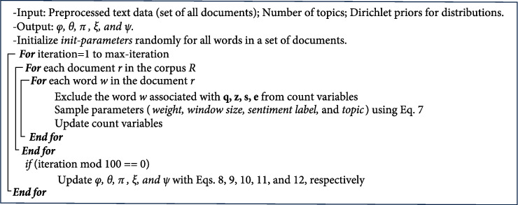
Adopted Gibbs sampling for WJST1.
In the section of initialization, the method randomly sets the parameters. A sentiment dictionary is employed for initializing sentiment labels. The sentiment dictionary contains words and scores that specify positive and negative labels and their weight. In this study, AFINN [64] is used as a sentiment dictionary, improving the model's accuracy. At the end of the sampling algorithm, each word has a weight and a sentiment label. Therefore, a dictionary can generate sentiment scores (weights and sentiment labels) and words. The scores are extracted from a dataset based on P(w| s, e). Each word's weight and sentiment with the most probability are selected as sentiment scores among all documents. Adaptive Lexicon learning using Genetic Algorithm (ALGA) [46] uses the genetic algorithm to generate a sentiment dictionary. However, we use topic modeling in WJST, to generate this dictionary. In WJST, the window size is different for various words. At each step of the sampling algorithm, count variables such as Fs,r and Fr are updated after sampling sentiment label, weight, and window size. After completing the sampling, the distribution of latent variables (φ, θ, π, ξ, and ψ) can be calculated as follows:
| (8) |
| (9) |
| (10) |
| (11) |
The probability of a word given a topic would be equal to, and the probability of a sentiment label given a document for sentiment classification at the document-level is calculated using π.
The time complexity of the proposed method quantifies the amount of time taken by the Gibbs sampling algorithm to run as the main function. Given the number of words in all documents wALL (wALL=∑r∈RNr, where Nr is the number of words in document r), the number of topics |Z|, the number of distinct windows |Q|, the number of weights |E|, and the total number of sentiment labels |S|, the time complexity of each Gibbs sampling iteration would be O(wALL·|S|·|Z|·|Q|·|E|). Furthermore, given the number of iterations G, the total time complexity of WJST would be O(G·wALL·|S|·|Z|·|Q|·|E|). Table 3 compares different methods in terms of time complexity.
Table 3.
The time complexity of different models.
| Model | Time complexity |
|---|---|
| JST, RJST, TJST, and TS | O(G· wALL·|S|·|Z|) |
| WJST | O(G· wALL·|S|·|Z|·|Q|·|E|) |
3.4. The General Structure of WJST1
A version of WJST called WJST1 is presented in Figure 7. The distributions θ, ξ, and ψ in WJST depend on the document, but in WJST1, the distributions θ, ξ, and ψ do not rely on the document. Dependency between documents of a domain is more than documents in different domains. A pattern in documents of a domain may not exist in documents of other domains. So, calculations on multidomain datasets should be local and not cover all domains. For example, considering the distributions P(z| s) and P(z| s, r), where z is topic, s is sentiment, and r documents, in the first state P(z| s), topic depends on sentiment. The distribution covers all documents in different domains. Perhaps a topic is positive in one domain and negative in another domain. So, it is better to depend the topic on the documents of a domain, not all domains. Thus, the topic is limited to the document (and domain), and contradiction between different domains is eliminated. So, WJST is suitable for multidomain datasets, and WJST1 is a version of WJST suitable for single-domain datasets. According to Figure 7, ξ is the probability of q given z, θ is the probability of z given s, and ψ is the probability of e given z and s, and the joint probability distribution for WJST1 can be factored as follows:
| (12) |
where by integrating out θ, we achieve:
| (13) |
where Nz,s is the number of words with topic z and sentiment s. The symbol Ns is the number of words with sentiment s. The symbol α is Dirichlet before θ. And by integrating out ξ, we achieve:
| (14) |
where Nq,z is the number of words with topic z and window q. The symbol Nz is the number of words with topic z. The symbol μ is Dirichlet before ξ. And by integrating out ψ, we achieve:
| (15) |
where Ne,z,s is the number of words with topic z, weight e, and sentiment s. The symbol Nz,s is the number of words with sentiment s and topic z. The symbol δ is Dirichlet before ψ. The symbols P(w| z, s, q, e) and P(s| r) are calculated using equations (2) and (4), respectively. After completing the sampling, the distribution of latent variables (θ, ξ, and ψ) is calculated as follows:
| (16) |
Figure 7.

The graphical model of WJST1.
And φ and π are computed through equations (8) and (10), respectively. Experimental results are demonstrated in the next section.
4. Experimental Results
The present study executes the methods on a computer with an Intel Core i7 CPU and 8 GB RAM. Proposed models are compared on 13 datasets. 4 datasets crawled from Amazon (https://www.amazon.com) opinions include Electronic, Movie, Android, and Automotive. 2 MDS datasets [65] contain Magazines and Sports. A dataset crawled from the IMDB movie archive [3] is MR. 3 UCI datasets [66] include Amazon, Yelp, and IMDB. 3 Twitter datasets [46] include STS-Test, SOMD, and Sanders. Data preprocessing contains (1) lowercasing all words, (2) removing digits, nonalphabetic characters, stop words, and words with too low and too high frequency, and (3) stemming. The details of the datasets are provided in Table 4.
Table 4.
Description of datasets.
| # | Dataset | Number of reviews | Vocabulary size | Number of words |
|---|---|---|---|---|
| 1 | Movie | 400 | 6592 | 41540 |
| 2 | Electronic | 400 | 4501 | 29117 |
| 3 | Automotive | 400 | 3590 | 19733 |
| 4 | Android | 400 | 2173 | 9723 |
| 5 | STS | 359 | 1489 | 3784 |
| 6 | SOMD | 916 | 2013 | 7772 |
| 7 | Sanders | 1224 | 3221 | 14100 |
| 8 | Magazines | 1800 | 8040 | 125387 |
| 9 | Sports | 2000 | 8582 | 113921 |
| 10 | MR | 2000 | 33054 | 733022 |
| 11 | Amazon | 1000 | 1521 | 7296 |
| 12 | IMDB | 1000 | 2556 | 9706 |
| 13 | Yelp | 1000 | 1679 | 7726 |
The number of topics is unknown, provided as a constant amount at the beginning of the Gibbs sampling algorithm. In this study, α, γ, β, and δ specific distributions are symmetric, and we empirically set the value of parameters, and this setting demonstrates fairly good performance in our experiments. Table 5 exhibits the initialization of parameters used in different algorithms.
Table 5.
Initial values of parameters.
| Model | Parameters |
|---|---|
| JST | Max_iteration:5000; |Z| = 5,10,15,20; α=0.1; γ=0.016 × (average document length); β=0.01; |
| RJST | Max_iteration:5000; |Z| = 5,10,15,20; α=0.1; γ=0.016 × (average document length); β=0.01; |
| TJST | Max_iteration:5000; |Z| = 5,10,15,20; α=0.1; γ=0.016 × (average document length); β=0.01; |
| TS | Max_iteration:5000; |Z| = 5,10,15,20; α=0.1; γ=0.016 × (average document length); β=0.01; |
| WJST | Max_iteration:5000; |Z| = 5,10,15,20; α=0.3; γ=0.016 × (average document length); β=0.01; μ=3; δ=9; E = [−5, +5]; Q = {1,2,3,4,5,6}; |
| WJST1 | Max_iteration:5000;
|Z| = 5,10,15,20;
α=0.3; γ=0.016 ×
(average document length);
β=0.01; μ=3; δ=9; E = [−5, +5]; Q = {1,2,3,4,5,6}; |
A sentiment dictionary is employed for initializing sentiment labels. Sentiment dictionaries such as AFINN [64], IMDB [67], 8-K [67], and Bing Liu [68, 69] contain words and scores that specify positive and negative labels as well as their weight. In the present study, AFINN is used as a sentiment dictionary which improves the model's accuracy. Sentiment detection at the document-level, perplexity, and topic_coherency are used to compare the efficacy of proposed models as three standard parameters which are used in different papers [7, 70, 71–73].
In the present study, the Accuracy parameter uses the formula of ((TP + TN))⁄((TP + FP + TN + FN)), where TP is the number of true positives, TN is the number of true negatives, FP is the number of false positives, and FN is the number of false negatives.
π distribution equation (10) determines how likely each comment is positive or negative. For example, if the value of P(+) is more significant than the value of P(−) (for a comment), the comment will be positive. The Accuracy's formula uses π distribution (equation (10)) to calculate TP, TN, FP, and FN values. For example, if a comment is positive and detected as positive (by the proposed methods), a unit is added to TP.
So, sentiment analysis (sentiment detection) at the document-level is realized using π distribution (equation (10)), and the formula of ((TP + TN))⁄((TP + FP + TN + FN)) is used to compute the Accuracy.
The error formula can be calculated using the formula of (1-Accuracy). Accuracy, perplexity, and topic_coherency are used for evaluations in the present study. Further study can investigate more parameters such as MSE, MAE, and RMSE for future research.
Furthermore, Better methods have lower perplexity and also higher topic_coherency. Given a test dataset DTest, the perplexity is computed through
| (17) |
where wr are the words in document r, Nr is the length of document r, and P(wr) is the probability of words in document r. The lower value of the formula over a held-out document demonstrates Better generalization efficacy. The evaluation results are shown in Tables 6–8, 9–14, and the proposed models demonstrate better results. In the report of Tables 6–8, 9–14, the perplexity of proposed methods is lower than that of baseline models. In the report of Tables 9–12, the perplexity is reduced with an increase in topics. Topic_coherency is also calculated using
| (18) |
where V(zi)=(v1(zi),…, vM(zi)) is the list of M words that have a high probability in the topic zi, C(V(zi)) is topic_coherency for the topic zi, Z is the set of all topics, |Z| is the number of distinct topics, DF is the document frequency, and CODF is the co-occurrence of two words in different documents. A smoothing count of 1 is included to avoid taking the logarithm of zero. In the present study, topic_coherency is computed through (18), equal to the average of topic_coherency values in Z. Furthermore, a higher value of topic_coherency reflects the better quality of the detected topics. M is equal to 10, and results are demonstrated in Tables 6–8, 9–14. A different number of topics (5, 10, 15, and 20) and different distinct windows (1, 2, 3, 4, 5, and 6) are applied for evaluating models. In this part, baseline methods include JST [8], RJST [10], TJST [8], and TS [9]. In the present section, the Friedman test [74, 75] is used to examine the achievements of the comparison methods. The Friedman test is a nonparametric multiple comparison test utilized to examine the differences between algorithms by assigning the lowest rank to the best approach in minimization problems and the highest rank to the best approach in maximization problems.
Table 6.
Sentiment classification on Android, Automotive, Electronic, and Movie datasets.
| Android | |||||||||
|---|---|---|---|---|---|---|---|---|---|
| Metric\ model | RND | AFINN | RND + AFINN | JST | TJST | RJST | TS | WJST | WJST1 |
| Accuracy1 | 0.48 | 0.6975 | 0.58 | 0.625 | 0.765 | 0.5825 | 0.5425 | 0.795 | 0.865 |
| Accuracy2 | — | — | — | — | — | — | — | 0.7825 | 0.8525 |
| Perplexity | — | — | — | 17.4581 | 19.7185 | 17.4426 | 17.8706 | 14.396 | 14.7631 |
| Topic_coherency | — | — | — | −2.0645 | −0.8536 | −1.9914 | −2.373 | −0.5547 | −0.187 |
|
| |||||||||
| Automotive | |||||||||
| Accuracy1 | 0.4925 | 0.625 | 0.535 | 0.6575 | 0.7675 | 0.615 | 0.5525 | 0.755 | 0.8 |
| Accuracy2 | — | — | — | — | — | — | — | 0.7475 | 0.795 |
| Perplexity | — | — | — | 22.6838 | 24.0385 | 21.8044 | 22.4878 | 18.4612 | 19.0627 |
| Topic_coherency | — | — | — | −1.0158 | −0.4712 | −1.4986 | −0.9008 | −0.9311 | −0.326 |
|
| |||||||||
| Electronic | |||||||||
| Accuracy1 | 0.465 | 0.675 | 0.52 | 0.7025 | 0.76 | 0.5525 | 0.5475 | 0.8625 | 0.8475 |
| Accuracy2 | — | — | — | — | — | — | — | 0.875 | 0.855 |
| Perplexity | — | — | — | 23.3586 | 24.3024 | 23.471 | 24.0239 | 19.2999 | 20.2452 |
| Topic_coherency | — | — | — | −1.5892 | −1.0482 | −1.2996 | −1.2719 | −0.5322 | −1.1683 |
|
| |||||||||
| Movie | |||||||||
| Accuracy1 | 0.525 | 0.595 | 0.555 | 0.7575 | 0.9475 | 0.62 | 0.5425 | 0.8475 | 0.97 |
| Accuracy2 | — | — | — | — | — | — | — | 0.8325 | 0.9675 |
| Perplexity | — | — | — | 25.2787 | 26.5813 | 25.1684 | 25.4488 | 21.0494 | 22.1082 |
| Topic_coherency | — | — | — | −0.4089 | −0.111 | −1.0947 | −1.0214 | −0.0602 | −0.1329 |
Table 7.
Sentiment classification on Magazine, Sport, MR, Amazon, IMDB, and Yelp datasets.
| Magazine | |||||||||
|---|---|---|---|---|---|---|---|---|---|
| Metric\ model | RND | AFINN | RND + AFINN | JST | TJST | RJST | TS | WJST | WJST1 |
| Accuracy1 | 0.515 | 0.6522 | 0.5822 | 0.6705 | 0.705 | 0.5411 | 0.5022 | 0.8355 | 0.81 |
| Accuracy2 | — | — | — | — | — | — | — | 0.8372 | 0.8083 |
| Perplexity | — | — | — | 21.8506 | 23.0349 | 21.4593 | 21.3828 | 19.9914 | 21.2095 |
| Topic_coherency | — | — | — | −0.0548 | −0.0348 | −0.0946 | −0.0561 | −0.132 | −0.0077 |
|
| |||||||||
| Sport | |||||||||
| Accuracy1 | 0.5285 | 0.686 | 0.5725 | 0.653 | 0.709 | 0.5565 | 0.5155 | 0.798 | 0.802 |
| Accuracy2 | — | — | — | — | — | — | — | 0.782 | 0.795 |
| Perplexity | — | — | — | 22.874 | 23.1356 | 22.0264 | 22.3361 | 21.968 | 21.4821 |
| Topic_coherency | — | — | — | −0.2234 | −0.0876 | −0.1369 | −0.0544 | −0.1406 | −0.2242 |
|
| |||||||||
| MR | |||||||||
| Accuracy1 | 0.4895 | 0.601 | 0.5455 | 0.613 | 0.62 | 0.51 | 0.5 | 0.821 | 0.8445 |
| Accuracy2 | — | — | — | — | — | — | — | 0.818 | 0.843 |
| Perplexity | — | — | — | 33.8663 | 35.0695 | 35.2359 | 34.6704 | 33.222 | 33.7698 |
| Topic_coherency | — | — | — | −0.021 | −0.0139 | −0.0012 | −0.0409 | −0.001 | −0.0106 |
|
| |||||||||
| Amazon | |||||||||
| Accuracy1 | 0.491 | 0.731 | 0.574 | 0.611 | 0.645 | 0.609 | 0.54 | 0.779 | 0.796 |
| Accuracy2 | — | — | — | — | — | — | — | 0.829 | 0.798 |
| Perplexity | — | — | — | 12.6442 | 13.7316 | 13.349 | 14.2397 | 10.9211 | 12.9946 |
| Topic_coherency | — | — | — | −0.8318 | −4.3775 | −0.4224 | −0.5411 | −0.5874 | −0.2696 |
|
| |||||||||
| IMDB | |||||||||
| Accuracy1 | 0.498 | 0.698 | 0.575 | 0.605 | 0.616 | 0.546 | 0.545 | 0.76 | 0.77 |
| Accuracy2 | — | — | — | — | — | — | — | 0.761 | 0.774 |
| Perplexity | — | — | — | 21.1053 | 20.4419 | 20.8543 | 19.7124 | 14.6719 | 18.9035 |
| Topic_coherency | — | — | — | −1.3334 | −1.4868 | −0.8853 | −1.1246 | −0.9666 | −0.9438 |
|
| |||||||||
| Yelp | |||||||||
| Accuracy1 | 0.506 | 0.689 | 0.559 | 0.579 | 0.614 | 0.561 | 0.547 | 0.737 | 0.773 |
| Accuracy2 | — | — | — | — | — | — | — | 0.726 | 0.769 |
| Perplexity | — | — | — | 15.4565 | 16.7169 | 15.5965 | 15.3614 | 12.2145 | 13.3453 |
| Topic_coherency | — | — | — | −2.1865 | −2.5609 | −1.9632 | −1.1714 | −2.0815 | −2.3715 |
Table 8.
Sentiment classification on different datasets based on different situations (AFINN and NO_AFINN).
| Android | |||
|---|---|---|---|
| Metric | Metric\Dic | AFINN | NO_AFINN |
| WJST | Accuracy1 | 0.7425 | 0.5725 |
| Accuracy2 | 0.7375 | 0.58 | |
| Perplexity | 15.53 | 16.1551 | |
| Topic_Coh | −2.2654 | −1.7346 | |
| WJST1 | Accuracy1 | 0.855 | 0.81 |
| Accuracy2 | 0.8475 | 0.8075 | |
| Perplexity | 16.3399 | 16.0482 | |
| Topic_Coh | −2.2228 | −0.1295 | |
|
| |||
| Automotive | |||
| WJST | Accuracy1 | 0.7125 | 0.6025 |
| Accuracy2 | 0.7025 | 0.6075 | |
| Perplexity | 20.4488 | 20.4065 | |
| Topic_Coh | −3.2282 | −1.6628 | |
| WJST1 | Accuracy1 | 0.7925 | 0.7025 |
| Accuracy2 | 0.79 | 0.7125 | |
| Perplexity | 20.5213 | 21.1296 | |
| Topic_Coh | −0.326 | −1.1809 | |
|
| |||
| Electronic | |||
| WJST | Accuracy1 | 0.8525 | 0.705 |
| Accuracy2 | 0.8425 | 0.6825 | |
| Perplexity | 20.0579 | 20.2615 | |
| Topic_Coh | −0.5322 | −0.5926 | |
| WJST1 | Accuracy1 | 0.8475 | 0.76 |
| Accuracy2 | 0.855 | 0.765 | |
| Perplexity | 21.8195 | 21.5739 | |
| Topic_Coh | −1.5586 | −1.6968 | |
|
| |||
| Movie | |||
| WJST | Accuracy1 | 0.8475 | 0.71 |
| Accuracy2 | 0.8325 | 0.715 | |
| Perplexity | 22.4588 | 22.6124 | |
| Topic_Coh | −0.9342 | −0.4637 | |
| WJST1 | Accuracy1 | 0.9575 | 0.485 |
| Accuracy2 | 0.945 | 0.4875 | |
| Perplexity | 23.5662 | 22.8134 | |
| Topic_Coh | −1.2359 | −1.3717 | |
Table 9.
Sentiment classification on the Android dataset according to the different number of topics.
| Model | Metric\topic | 5 | 10 | 15 | 20 |
|---|---|---|---|---|---|
| RND | Accuracy | 0.48 | 0.48 | 0.48 | 0.48 |
| AFINN | Accuracy | 0.6975 | 0.6975 | 0.6975 | 0.6975 |
| AFINN + RND | Accuracy | 0.58 | 0.58 | 0.58 | 0.58 |
| Bing_Liu | Accuracy | 0.6975 | 0.6975 | 0.6975 | 0.6975 |
| Bing_Liu + RND | Accuracy | 0.5775 | 0.5775 | 0.5775 | 0.5775 |
| IMDB | Accuracy | 0.7025 | 0.7025 | 0.7025 | 0.7025 |
| IMDB + RND | Accuracy | 0.6125 | 0.6125 | 0.6125 | 0.6125 |
| 8K | Accuracy | 0.5425 | 0.5425 | 0.5425 | 0.5425 |
| 8K + RND | Accuracy | 0.515 | 0.515 | 0.515 | 0.515 |
| JST | Accuracy | 0.625 | 0.6175 | 0.6225 | 0.6125 |
| Perplexity | 19.6726 | 19.5187 | 19.182 | 17.4581 | |
| Topic_Coh | −4.6026 | −2.5848 | −2.2753 | −2.0645 | |
| TJST | Accuracy | 0.7575 | 0.7175 | 0.765 | 0.7475 |
| Perplexity | 21.1487 | 20.3726 | 20.1516 | 19.7185 | |
| Topic_Coh | −0.8536 | −1.568 | −3.4285 | −2.8739 | |
| RJST | Accuracy | 0.5825 | 0.54 | 0.555 | 0.5325 |
| Perplexity | 19.9429 | 19.1915 | 18.137 | 17.4426 | |
| Topic_Coh | −3.3792 | −1.9914 | −3.403 | −3.4386 | |
| TS | Accuracy | 0.5425 | 0.5275 | 0.53 | 0.5175 |
| Perplexity | 20.4934 | 19.1762 | 18.3833 | 17.8706 | |
| Topic_Coh | −3.9618 | −3.2137 | −2.373 | −2.569 | |
| WJST | Accuracy1 | 0.7925 | 0.7425 | 0.795 | 0.79 |
| Accuracy2 | 0.7775 | 0.7375 | 0.775 | 0.7825 | |
| Perplexity | 16.7303 | 15.53 | 14.6351 | 14.396 | |
| Topic_Coh | −0.5547 | −2.2654 | −2.9122 | −2.6465 | |
| WJST1 | Accuracy1 | 0.81 | 0.855 | 0.865 | 0.85 |
| Accuracy2 | 0.7925 | 0.8475 | 0.8525 | 0.8375 | |
| Perplexity | 16.6787 | 16.3399 | 15.6662 | 14.7631 | |
| Topic_Coh | −0.187 | −2.2228 | −1.5703 | −2.0204 |
Table 10.
Sentiment classification on the Automotive dataset according to the different number of topics.
| Model | Metric\topic | 5 | 10 | 15 | 20 |
|---|---|---|---|---|---|
| RND | Accuracy | 0.4925 | 0.4925 | 0.4925 | 0.4925 |
| AFINN | Accuracy | 0.625 | 0.625 | 0.625 | 0.625 |
| AFINN + RND | Accuracy | 0.535 | 0.535 | 0.535 | 0.535 |
| Bing_Liu | Accuracy | 0.64 | 0.64 | 0.64 | 0.64 |
| Bing_Liu + RND | Accuracy | 0.535 | 0.535 | 0.535 | 0.535 |
| IMDB | Accuracy | 0.59 | 0.59 | 0.59 | 0.59 |
| IMDB + RND | Accuracy | 0.4825 | 0.4825 | 0.4825 | 0.4825 |
| 8K | Accuracy | 0.5025 | 0.5025 | 0.5025 | 0.5025 |
| 8K + RND | Accuracy | 0.48 | 0.48 | 0.48 | 0.48 |
| JST | Accuracy | 0.6275 | 0.6575 | 0.6325 | 0.5975 |
| Perplexity | 24.7154 | 23.6961 | 23.27 | 22.6838 | |
| Topic_Coh | −1.486 | −2.3443 | −1.1354 | −1.0158 | |
| TJST | Accuracy | 0.76 | 0.7375 | 0.7675 | 0.7275 |
| Perplexity | 25.5637 | 25.0633 | 24.5749 | 24.0385 | |
| Topic_Coh | −0.59 | −0.4712 | −1.6252 | −1.9377 | |
| RJST | Accuracy | 0.615 | 0.55 | 0.54 | 0.535 |
| Perplexity | 25.2654 | 23.8316 | 22.3905 | 21.8044 | |
| Topic_Coh | −1.5779 | −1.4986 | −2.0833 | −2.9936 | |
| TS | Accuracy | 0.5425 | 0.5375 | 0.5525 | 0.55 |
| Perplexity | 25.0705 | 23.8504 | 22.9364 | 22.4878 | |
| Topic_Coh | −2.5941 | −0.9008 | −6.2652 | −4.6902 | |
| WJST | Accuracy1 | 0.755 | 0.7125 | 0.74 | 0.745 |
| Accuracy2 | 0.7475 | 0.7025 | 0.745 | 0.735 | |
| Perplexity | 21.2008 | 20.4488 | 18.7049 | 18.4612 | |
| Topic_Coh | −1.6542 | −3.2282 | −1.6783 | −0.9311 | |
| WJST1 | Accuracy1 | 0.80 | 0.7925 | 0.7925 | 0.7925 |
| Accuracy2 | 0.79 | 0.79 | 0.79 | 0.795 | |
| Perplexity | 21.4357 | 20.5213 | 20.0481 | 19.0627 | |
| Topic_Coh | −1.1883 | −0.326 | −1.084 | −0.8349 |
Table 11.
Sentiment classification on the Electronic dataset according to the different number of topics.
| Model | Metric\topic | 5 | 10 | 15 | 20 |
|---|---|---|---|---|---|
| RND | Accuracy | 0.465 | 0.465 | 0.465 | 0.465 |
| AFINN | Accuracy | 0.675 | 0.675 | 0.675 | 0.675 |
| AFINN + RND | Accuracy | 0.52 | 0.52 | 0.52 | 0.52 |
| Bing_Liu | Accuracy | 0.695 | 0.695 | 0.695 | 0.695 |
| Bing_Liu + RND | Accuracy | 0.535 | 0.535 | 0.535 | 0.535 |
| IMDB | Accuracy | 0.6375 | 0.6375 | 0.6375 | 0.6375 |
| IMDB + RND | Accuracy | 0.5475 | 0.5475 | 0.5475 | 0.5475 |
| 8K | Accuracy | 0.5075 | 0.5075 | 0.5075 | 0.5075 |
| 8K + RND | Accuracy | 0.5075 | 0.5075 | 0.5075 | 0.5075 |
| JST | Accuracy | 0.675 | 0.7025 | 0.6475 | 0.6275 |
| Perplexity | 25.227 | 24.6719 | 24.6115 | 23.3586 | |
| Topic_Coh | −1.5892 | −4.1751 | −2.6007 | −2.1239 | |
| TJST | Accuracy | 0.75 | 0.74 | 0.73 | 0.76 |
| Perplexity | 25.2091 | 24.8028 | 24.4092 | 24.3024 | |
| Topic_Coh | −1.0482 | −1.8084 | −1.6694 | −1.8297 | |
| RJST | Accuracy | 0.5525 | 0.55 | 0.5375 | 0.53 |
| Perplexity | 25.3113 | 24.1779 | 23.8378 | 23.471 | |
| Topic_Coh | −1.2996 | −1.3991 | −4.472 | −5.4363 | |
| TS | Accuracy | 0.54 | 0.5375 | 0.5475 | 0.515 |
| Perplexity | 26.2295 | 24.885 | 24.5048 | 24.0239 | |
| Topic_Coh | −1.2719 | −1.6586 | −2.5403 | −3.2174 | |
| WJST | Accuracy1 | 0.8625 | 0.8525 | 0.7675 | 0.675 |
| Accuracy2 | 0.875 | 0.8425 | 0.755 | 0.665 | |
| Perplexity | 20.5489 | 20.0579 | 19.9009 | 19.2999 | |
| Topic_Coh | −2.0442 | −0.5322 | −1.3702 | −1.0887 | |
| WJST1 | Accuracy1 | 0.79 | 0.8475 | 0.8075 | 0.8275 |
| Accuracy2 | 0.80 | 0.855 | 0.8125 | 0.8225 | |
| Perplexity | 22.6012 | 21.8195 | 20.8551 | 20.2452 | |
| Topic_Coh | −1.1683 | −1.5586 | −1.6646 | −1.4681 |
Table 12.
Sentiment classification on the Movie dataset according to the different number of topics.
| Model | Metric\topic | 5 | 10 | 15 | 20 |
|---|---|---|---|---|---|
| RND | Accuracy | 0.525 | 0.525 | 0.525 | 0.525 |
| AFINN | Accuracy | 0.595 | 0.595 | 0.595 | 0.595 |
| AFINN + RND | Accuracy | 0.555 | 0.555 | 0.555 | 0.555 |
| Bing_Liu | Accuracy | 0.635 | 0.635 | 0.635 | 0.635 |
| Bing_Liu + RND | Accuracy | 0.565 | 0.565 | 0.565 | 0.565 |
| IMDB | Accuracy | 0.6425 | 0.6425 | 0.6425 | 0.6425 |
| IMDB + RND | Accuracy | 0.5975 | 0.5975 | 0.5975 | 0.5975 |
| 8K | Accuracy | 0.5025 | 0.5025 | 0.5025 | 0.5025 |
| 8K + RND | Accuracy | 0.51 | 0.51 | 0.51 | 0.51 |
| JST | Accuracy | 0.7575 | 0.6375 | 0.7175 | 0.6325 |
| Perplexity | 27.3111 | 26.9145 | 26.2463 | 25.2787 | |
| Topic_Coh | −1.0123 | −0.4089 | −1.2434 | −1.226 | |
| TJST | Accuracy | 0.915 | 0.9425 | 0.9475 | 0.9325 |
| Perplexity | 27.791 | 27.4122 | 26.993 | 26.5813 | |
| Topic_Coh | −0.111 | −1.6632 | −0.199 | −0.8503 | |
| RJST | Accuracy | 0.62 | 0.54 | 0.5175 | 0.5175 |
| Perplexity | 27.6284 | 26.5172 | 26.1489 | 25.1684 | |
| Topic_Coh | −2.6713 | −1.0947 | −1.979 | −2.3544 | |
| TS | Accuracy | 0.5425 | 0.515 | 0.5175 | 0.5175 |
| Perplexity | 27.6707 | 26.4786 | 26.1138 | 25.4488 | |
| Topic_Coh | −1.5025 | −1.3799 | −1.0214 | −4.6598 | |
| WJST | Accuracy1 | 0.7225 | 0.8475 | 0.7525 | 0.6975 |
| Accuracy2 | 0.71 | 0.8325 | 0.7575 | 0.6875 | |
| Perplexity | 23.1145 | 22.4588 | 21.2982 | 21.0494 | |
| Topic_Coh | −0.0751 | −0.9342 | −0.0602 | −0.4873 | |
| WJST1 | Accuracy1 | 0.97 | 0.9575 | 0.9675 | 0.9675 |
| Accuracy2 | 0.9625 | 0.945 | 0.9675 | 0.96 | |
| Perplexity | 24.6302 | 23.5662 | 22.7180 | 22.1082 | |
| Topic_Coh | −0.1348 | −1.2359 | −0.1329 | −0.7102 |
Table 13.
Sentiment classification on different datasets according to the different number of distinct windows (before random selection).
| Android | |||||||
|---|---|---|---|---|---|---|---|
| Model | Metric\window | 1 | 2 | 3 | 4 | 5 | 6 |
| WJST | Accuracy1 | 0.8375 | 0.78 | 0.7925 | 0.7425 | 0.725 | 0.9075 |
| Accuracy2 | 0.83 | 0.77 | 0.7775 | 0.735 | 0.725 | 0.9075 | |
| Perplexity | 18.3948 | 16.7266 | 16.7303 | 16.166 | 15.9499 | 15.1128 | |
| Topic_Coh | −1.4063 | −0.9279 | −0.5547 | −1.2929 | −1.7475 | −0.746 | |
| WJST1 | Accuracy1 | 0.8975 | 0.8525 | 0.81 | 0.8675 | 0.755 | 0.8025 |
| Accuracy2 | 0.8825 | 0.83 | 0.7925 | 0.8675 | 0.75 | 0.7875 | |
| Perplexity | 19.3734 | 18.0031 | 16.6787 | 16.8518 | 16.1015 | 16.5461 | |
| Topic_Coh | −2.2084 | −1.6272 | −0.1870 | −0.7753 | −1.328 | −1.7836 | |
|
| |||||||
| Automotive | |||||||
| WJST | Accuracy1 | 0.7775 | 0.74 | 0.755 | 0.735 | 0.7375 | 0.69 |
| Accuracy2 | 0.7725 | 0.745 | 0.7475 | 0.745 | 0.725 | 0.685 | |
| Perplexity | 23.6365 | 21.7712 | 21.2008 | 20.9688 | 20.5095 | 19.6748 | |
| Topic_Coh | −1.1684 | −1.7095 | −1.6542 | −0.2824 | −1.7604 | −0.1311 | |
| WJST1 | Accuracy1 | 0.805 | 0.8125 | 0.8 | 0.7575 | 0.78 | 0.7725 |
| Accuracy2 | 0.805 | 0.7975 | 0.79 | 0.755 | 0.78 | 0.7725 | |
| Perplexity | 23.2684 | 22.2601 | 21.4357 | 20.8092 | 20.5091 | 20.2379 | |
| Topic_Coh | −1.7318 | −0.5912 | −1.1883 | −0.7637 | −0.62 | −0.5134 | |
|
| |||||||
| Electronic | |||||||
| WJST | Accuracy1 | 0.845 | 0.7675 | 0.8625 | 0.7325 | 0.7775 | 0.7325 |
| Accuracy2 | 0.845 | 0.7575 | 0.875 | 0.7275 | 0.7825 | 0.7225 | |
| Perplexity | 22.561 | 22.0462 | 20.5489 | 20.7952 | 20.7495 | 20.0283 | |
| Topic_Coh | −0.8471 | −0.6207 | −2.0442 | −1.4345 | −0.786 | −0.9412 | |
| WJST1 | Accuracy1 | 0.8025 | 0.875 | 0.79 | 0.8675 | 0.8625 | 0.835 |
| Accuracy2 | 0.7975 | 0.87 | 0.8 | 0.865 | 0.8625 | 0.8375 | |
| Perplexity | 23.5903 | 23.546 | 22.6012 | 22.8559 | 21.8897 | 21.4464 | |
| Topic_Coh | −0.8251 | −0.9581 | −1.1683 | −1.2189 | −0.8492 | −0.3402 | |
|
| |||||||
| Movie | |||||||
| WJST | Accuracy1 | 0.855 | 0.815 | 0.7225 | 0.6575 | 0.7 | 0.765 |
| Accuracy2 | 0.845 | 0.7975 | 0.71 | 0.6625 | 0.685 | 0.765 | |
| Perplexity | 24.5779 | 24.5153 | 23.1145 | 23.1209 | 23.2709 | 22.2328 | |
| Topic_Coh | −0.4063 | −0.0216 | −0.0751 | −2.5351 | −0.0888 | −0.0791 | |
| WJST1 | Accuracy1 | 0.9725 | 0.9775 | 0.97 | 0.965 | 0.575 | 0.595 |
| Accuracy2 | 0.96 | 0.965 | 0.9625 | 0.955 | 0.5875 | 0.5725 | |
| Perplexity | 26.117 | 25.09 | 24.6302 | 23.9778 | 22.7068 | 22.3572 | |
| Topic_Coh | −0.1348 | −0.1348 | −0.1348 | −0.0315 | −0.0378 | −0.0106 | |
|
| |||||||
| Average section | |||||||
| WJST | Accuracy1 | 0.8287 | 0.7756 | 0.7831 | 0.7168 | 0.735 | 0.7737 |
| Accuracy2 | 0.8231 | 0.7675 | 0.7775 | 0.7175 | 0.7293 | 0.77 | |
| Perplexity | 22.2925 | 21.2648 | 20.3986 | 20.2627 | 20.1199 | 19.2621 | |
| Topic_Coh | −0.957 | −0.8199 | −1.082 | −1.3862 | −1.0956 | −0.4743 | |
| WJST1 | Accuracy1 | 0.8693 | 0.8793 | 0.8425 | 0.8643 | 0.7431 | 0.7512 |
| Accuracy2 | 0.8612 | 0.8656 | 0.8362 | 0.8606 | 0.745 | 0.7425 | |
| Perplexity | 23.0872 | 22.2248 | 21.3364 | 21.1236 | 20.3017 | 20.1469 | |
| Topic_Coh | −1.225 | −0.8278 | −0.6696 | −0.6973 | −0.7087 | −0.6619 | |
Table 14.
Sentiment classification on different datasets according to the different number of distinct windows (after random selection).
| Android | |||||||
|---|---|---|---|---|---|---|---|
| Model | Metric\window | 1 | 2 | 3 | 4 | 5 | 6 |
| WJST | Accuracy1 | 0.71 | 0.775 | 0.7025 | 0.69 | 0.7175 | 0.675 |
| Accuracy2 | 0.7 | 0.765 | 0.6975 | 0.68 | 0.705 | 0.6675 | |
| Perplexity | 17.791 | 15.8544 | 16.1124 | 15.6932 | 13.8904 | 14.1876 | |
| Topic_Coh | −1.6 | −1.9691 | −1.4526 | −4.6888 | −2.6353 | −1.2267 | |
| WJST1 | Accuracy1 | 0.8025 | 0.85 | 0.845 | 0.8025 | 0.8675 | 0.76 |
| Accuracy2 | 0.7925 | 0.83 | 0.84 | 0.7875 | 0.865 | 0.7525 | |
| Perplexity | 18.9319 | 17.7849 | 17.6145 | 15.8017 | 15.4004 | 15.0917 | |
| Topic_Coh | −1.2666 | −1.6744 | −3.027 | −2.3428 | −1.1215 | −2.0183 | |
|
| |||||||
| Automotive | |||||||
| WJST | Accuracy1 | 0.7425 | 0.7375 | 0.68 | 0.6825 | 0.6725 | 0.64 |
| Accuracy2 | 0.74 | 0.73 | 0.6775 | 0.68 | 0.6625 | 0.6325 | |
| Perplexity | 20.8433 | 20.7212 | 19.6843 | 20.0801 | 19.1691 | 18.7129 | |
| Topic_Coh | −1.4406 | −2.0489 | −2.6701 | −2.2155 | −1.1019 | −1.1651 | |
| WJST1 | Accuracy1 | 0.7825 | 0.76 | 0.755 | 0.7725 | 0.7475 | 0.7675 |
| Accuracy2 | 0.785 | 0.7575 | 0.7475 | 0.775 | 0.7525 | 0.76 | |
| Perplexity | 22.1856 | 21.3601 | 20.6057 | 19.8915 | 19.402 | 19.0827 | |
| Topic_Coh | −1.5638 | −1.474 | −1.1274 | −1.7761 | −1.2042 | −1.1755 | |
|
| |||||||
| Electronic | |||||||
| WJST | Accuracy1 | 0.7975 | 0.72 | 0.76 | 0.6875 | 0.7675 | 0.6825 |
| Accuracy2 | 0.795 | 0.715 | 0.7475 | 0.66 | 0.765 | 0.665 | |
| Perplexity | 21.9171 | 21.0509 | 20.4858 | 20.26 | 19.4089 | 19.5549 | |
| Topic_Coh | −0.8282 | −1.0407 | −0.9593 | −0.9779 | −1.0413 | −0.6259 | |
| WJST1 | Accuracy1 | 0.7475 | 0.7425 | 0.7775 | 0.7425 | 0.7725 | 0.78 |
| Accuracy2 | 0.745 | 0.7475 | 0.78 | 0.74 | 0.7625 | 0.785 | |
| Perplexity | 23.2269 | 22.4573 | 21.7203 | 21.4598 | 20.8683 | 20.5084 | |
| Topic_Coh | −1.7905 | −1.5082 | −1.4854 | −0.9143 | −1.2881 | −1.3489 | |
|
| |||||||
| Movie | |||||||
| WJST | Accuracy1 | 0.7425 | 0.77 | 0.8075 | 0.615 | 0.7 | 0.595 |
| Accuracy2 | 0.7425 | 0.765 | 0.7875 | 0.59 | 0.69 | 0.595 | |
| Perplexity | 23.7529 | 23.322 | 22.1056 | 21.8573 | 20.8467 | 20.9653 | |
| Topic_Coh | −1.0908 | −0.9134 | −0.9145 | −0.6129 | −1.1099 | −0.716 | |
| WJST1 | Accuracy1 | 0.9725 | 0.965 | 0.96 | 0.9675 | 0.96 | 0.9625 |
| Accuracy2 | 0.975 | 0.96 | 0.955 | 0.955 | 0.9575 | 0.9575 | |
| Perplexity | 26.1797 | 25.3138 | 24.5149 | 24.1116 | 23.5025 | 23.3023 | |
| Topic_Coh | −0.0218 | −0.2225 | −1.9033 | −0.0897 | −0.2896 | −0.0569 | |
|
| |||||||
| Average section | |||||||
| WJST | Accuracy1 | 0.7481 | 0.7506 | 0.7375 | 0.6687 | 0.7143 | 0.6481 |
| Accuracy2 | 0.7443 | 0.7437 | 0.7275 | 0.6525 | 0.7056 | 0.64 | |
| Perplexity | 21.076 | 20.2371 | 19.597 | 19.4726 | 18.3287 | 18.3551 | |
| Topic_Coh | −1.2399 | −1.493 | −1.4991 | −2.1237 | −1.4721 | −0.9334 | |
| WJST1 | Accuracy1 | 0.8262 | 0.8293 | 0.8343 | 0.8212 | 0.8368 | 0.8175 |
| Accuracy2 | 0.8243 | 0.8237 | 0.8306 | 0.8143 | 0.8343 | 0.8137 | |
| Perplexity | 22.631 | 21.729 | 21.1138 | 20.3161 | 19.7933 | 19.4962 | |
| Topic_Coh | −1.1606 | −1.2197 | −1.8857 | −1.2807 | −0.9758 | −1.1499 | |
There are several methods for the validation of classification and topic modeling-based problems. Still, the methods used in this study are the most common and are used in most articles related to our article for evaluation. Also, there are various methods for validation that we will try to use in a future study to evaluate the proposed methods. The following is the reason for choosing the validation methods used in this study:
We chose accuracy, perplexity, and coherence score as evaluation metrics because of their popularity in classification and topic modeling problems. Perplexity is an essential metric that, in theory, represents how well a model behaved on unseen data and is provided using the normalized log-likelihood technique. Meanwhile, the coherence score measures the degree of semantic similarity between high-scoring words and helps distinguish the semantical interpretation of topics based on statistical inference.
The main question we want to answer is whether the proposed methods can improve the performance of text sentiment classification. This study compares proposed methods with different baselines, including JST and recently representative approaches. Consider a Confusion Matrix for a classification problem that predicts whether a comment has positive sentiment or not. The total number of correctly detected cases is one of the more obvious measures. When all of the classes are equally important, it is typically utilized. When True positives and True negatives are more significant, accuracy is employed. According to the accuracy criterion, one can immediately know whether the model is adequately trained or not and how it works in general. The most popular measurement for classification issues is accuracy, which is the proportion of correctly predicted cases to all cases. This metric's opposite, or error, can be calculated as 1-accuracy. In machine learning, an accuracy parameter is an excellent option for sentiment classification when the classes in the dataset are almost evenly distributed. Also, we will try to use various metrics such as recall and precision in future studies to evaluate the proposed methods.
We use the Friedman test to compare the results produced by the proposed methods and the competitors to verify the classification performance. Friedman's test is used to examine the achievements of the comparison methods. The Friedman test is a nonparametric multiple comparison test that is utilized to explore the differences between algorithms by assigning the lowest rank to the best approach in minimization problems and the highest rank to the best approach in maximization problems.
Topic modeling is one of the most important NLP fields. It aims to explain a textual dataset by decomposing it into two distributions: topics and words. A topic modeling algorithm is a mathematical or statistical model used to infer what the issues that better represent the data are. Human judgment-based review techniques can yield good results but are expensive and time-consuming. Human judgment is also not well defined.
In contrast, the appeal of quantitative metrics such as perplexity is the ability to standardize, automate, and scale the evaluation of topic models. In natural language processing, perplexity is a traditional metric for evaluating topic models. The lower value of the formula over a held-out document demonstrates better generalization efficacy.
Perplexity's inability to capture context and the relationships between words within a topic or across topics within a document is one of its drawbacks. For human understanding, semantic context is important. Approaches like topic coherency have been designed to tackle this problem by capturing the context between words in a subject. Extracting topic words is one of the main tasks in topic modeling. In most articles about topic modeling, topic_coherency is shown as a number that represents the overall topics' interpretability and is used to assess the topics' quality. The higher the topic_coherency value, the better the quality of the subjects extracted.
4.1. Sentiment Scores for the Words in a Dataset
In this section, a dictionary is generated, including sentiment scores (weights and sentiment labels) and words. The scores are extracted from datasets based on P(w| s, e). The weight and sentiment with the most probability are selected for each word as a sentiment score. The extracted scores for some phrases in the form of unigram can be seen in Tables 15 and 16. ALGA [46] uses the genetic algorithm to generate a sentiment dictionary; however, we use topic modeling in the proposed models to create this dictionary. According to Tables 15 and 16, ten words from each dataset are selected and scored by the proposed models. For example, the word nice obtains a score of 4 in WJST and obtains a score of 5 in WJST1. The scores are different in the proposed methods; for example, the word serious achieves a score of 1 in WJST and a score of -2 in WJST1. Table 15 is related to Android, Automotive, Electronic, and Movie datasets. Table 16 is associated with STS, Sanders, and SOMD datasets.
Table 15.
Sentiment scores, for some instance, words related to Android, Automotive, Electronic, and Movie datasets.
| Dataset | Android | Automotive | Electronic | Movie | ||||
|---|---|---|---|---|---|---|---|---|
| Model | Word | Score | Word | Score | Word | Score | Word | Score |
| WJST1 | Nice | 5 | Much | 5 | Satisfy | 5 | See | 5 |
| Cute | 4 | Use | 4 | Crew | 4 | Father | 4 | |
| Favorit | 3 | Long | 3 | Way | 3 | Pray | 3 | |
| Perfect | 2 | Expens | 2 | Fluid | 2 | Human | 2 | |
| Great | 1 | Stuff | 1 | Feel | 1 | Event | 1 | |
| Type | −1 | Fals | −1 | Pull | −1 | Terribl | −1 | |
| Wast | −2 | Serious | −2 | Side | −2 | Sens | −2 | |
| Everi | −3 | Extens | −3 | Nervous | −3 | Lost | −3 | |
| Unknown | −4 | Space | −4 | Even | −4 | Sure | −4 | |
| Everyth | −5 | Know | −5 | Extend | −5 | Injur | −5 | |
|
| ||||||||
| WJST | Nice | 4 | Much | 3 | Satisfy | −2 | See | −4 |
| Cute | 1 | Use | 2 | Crew | 2 | Father | 5 | |
| Favorit | 2 | Long | 4 | Way | 4 | Pray | −3 | |
| Perfect | 2 | Expens | −4 | Fluid | 1 | Human | 5 | |
| Great | 2 | Stuff | −5 | Feel | −3 | Event | 1 | |
| Type | 1 | Fals | −5 | Pull | −4 | Terribl | 4 | |
| Wast | −5 | Serious | 1 | Side | −1 | Sens | −4 | |
| Everi | 4 | Extens | 5 | Nervous | 3 | Lost | 3 | |
| Unknown | 5 | Space | −5 | Even | −2 | Sure | 2 | |
| Everyth | 2 | Know | 4 | Extend | −5 | Injur | −5 | |
Table 16.
Sentiment scores for some instance words related to STS, Sanders, and SOMD datasets.
| Dataset | STS | Sanders | SOMD | |
|---|---|---|---|---|
| Model | Word | Score | Score | Score |
| WJST1 | Much | −4 | 4 | 2 |
| Good | 5 | 4 | −5 | |
| Bad | −5 | −1 | −5 | |
| Nice | −3 | 5 | 5 | |
| Hate | −5 | −5 | 1 | |
| Love | 5 | 5 | 3 | |
|
| ||||
| WJST | Much | −5 | −5 | −2 |
| Good | −4 | −1 | 3 | |
| Bad | −4 | −1 | 3 | |
| Nice | 3 | 2 | 1 | |
| Hate | −5 | −4 | 2 | |
| Love | 4 | −2 | −3 | |
4.2. Topic Discovery
The topics are extracted from datasets based on P(w|z) in this section. A topic is a multinomial distribution over words based on topics, sentiments, weights, and window sizes. The top words could approximately reflect the meaning of a topic. Tables 17–19 show some examples of topics extracted from Movie, Android, and Electronic datasets by different models. Each row shows the top 10 words for the corresponding topic and sentiment label. The top 10 words from each topic were extracted and then used for topic_coherency. Extracting topic words is one of the main tasks in topic modeling. This section lists the top 10 words in three examples for Movie, Android, and Electronic datasets. The listed words for each topic describe the topic. The listed words for the proposed methods have a better topic_coherency value than baseline methods because they have a higher value of topic_coherency. The higher the topic_coherency value, the better the quality of the subjects extracted.
Table 17.
Top 10 words extracted from the Movie dataset.
| Model | Sentiment | Top 10 words |
|---|---|---|
| WJST | + | jesu, film, God, love, mel, Christian, life, suffer, believ, roman |
| − | movi, godzilla, bad, dvd, origin, horror, buy, version, worst, actor | |
|
| ||
| WJST1 | + | Jesu, mel, passion, mother, stori, realli, great, everyon, God, like |
| − | godzilla, monster, go, time, star, know, kill, make, militari, American | |
|
| ||
| JST | + | mel, stori, mother, two, realli, becom, anoth, God, like, back |
| − | godzilla, look, monster, american, militari, like, worst, zellweg, emmerich, quit | |
Table 18.
Top 10 words extracted from Android dataset.
| Model | Sentiment | Top 10 words |
|---|---|---|
| WJST | + | app, game, sudoku, play, version, enjoy, option, want, hint, like |
| − | work, app, would, fire, live, station, tri, say, select, kindl, load, user | |
|
| ||
| WJST1 | + | sudoku, tri, love, game, time, easi, tablet, star, call, make |
| − | close, tablet, seem, get, year, download, much, station, time, android | |
|
| ||
| JST | + | station, want, even, peopl, work, avail, version, puzzl, custom, believ |
| − | use, app, find, review, great, got, total, new, night, fake | |
Table 19.
Top 10 words extracted from Electronic dataset.
| Model | Sentiment | Top 10 words |
|---|---|---|
| WJST | + | read, book, screen, touch, kindl, page, better, wifi, ebook, like |
| − | work, went, new, servic, need, bad, system, hous, number, mine | |
|
| ||
| WJST1 | + | googl, amazon, book, color, store, kindl, download, small, pdf |
| − | time, work, two, much, one, power, comput, phone, go, unit | |
|
| ||
| JST | + | book, touch, read, page, free, librari, touch, screen, much, pdf |
| − | plug, work, could, devic, comput, charger, router, cabl, item, design | |
4.3. Sentiment Classification at Document-Level
In this section, the number of distinct windows is three, and the models use the AFINN sentiment dictionary in the initialization section of the Gibbs sampling algorithm. A document is classified based on P(s| r), which is the probability of a sentiment given by a document. A document is classified as negative if P(+|r) < P(−| r) and vice versa. Determining sentiment is important which is calculated using two formulas in this paper. In the first formula, P(s| r)=Ns,r/Nr where Ns,r is the number of words with sentiment s in document r and Nr is the number of words in document r. In the second formula, P(s| r)=Fs,r/Fr where Fs,r is the effect of words with sentiment s in document r and Fr is equal to the sum of the effect of words with different sentiments in document r. In all evaluations, accuracy1 is calculated based on the first formula, and accuracy2 is calculated based on the second formula. As shown in Figure 8, the document is negative according to the first formula, and the document is positive according to the second formula, and the weight of positive words is more than negative ones, although the number of negative words is more than positive ones, and positive words can affect sentiment analysis at document-level.
Figure 8.

An example of calculating the sentiment of a document using two formulas.
In this section, the best values for each method (the highest accuracy, the lowest perplexity, and the highest topic_coherency) are selected from Tables 9–12 and are listed in Tables 6 and 7. Table 6 compares the models based on four datasets (Android, Automotive, Movie, and Electronic) and Table 7 compares the models based on six datasets (Magazine, Sports, MR, Amazon, IMDB, and Yelp). The results of Tables 6 and 7 are evaluated on unigram words. AFINN method classifies each document according to the P(s|r)=Ns,r/Nr where the word sentiment label is directly obtained from the AFINN sentiment lexicon. The RND method classifies each document according to the P(s|r)=Ns,r/Nr where the word sentiment label is determined randomly, and in the AFINN + RND method, the algorithm uses both AFINN and RND methods. The improvement over these methods will reflect how much the proposed methods and baseline methods can learn from a dataset. The report in Tables 6 and 7 shows that the proposed models perform better than JST. Based on the results, the proposed methods have a significant improvement over AFINN and the baseline methods on all datasets. As seen from AFINN-based methods results, the results calculated based on the sentiment lexicon are below 70% for most datasets. In this study, parameters perplexity and topic_coherency are not calculated for AFINN, RND, and AFINN + RND methods. TS and RJST methods have lower accuracy than other methods on all datasets, but JST and TJST achieve better performance. As can be seen from the results, TJST outperforms JST on all datasets because, in JST, the distribution θ depends on the document, but in TJST, the distribution θ does not depend on the document and is generally estimated because it uses all documents for computations. According to Tables 6 and 7, WJST1 has higher accuracy than other methods. WJST1 outperforms WJST because, in WJST, the distributions θ, ξ, and ψ depend on the document, but in WJST1, the distributions θ, ξ, and ψ do not depend on the document and are generally estimated because they use all documents for computations. The perplexity value varies on different datasets because the size of datasets is different, according to Table 4.
The analysis of the Friedman test on the results of Tables 6 and 7 demonstrates that there is a statistically significant difference between the performances of the algorithms in terms of accuracy with χ2(10)=92.091 and p < 0.01, in terms of perplexity with χ2(5)=38.629 and p < 0.01, and in terms of topic_coherency with χ2(5)=5.508 and p > 0.1. The mean rank of the algorithms based on the Friedman test, which is demonstrated in Figure 9, indicates that WJST1 ranks first among all the algorithms in 7 in terms of accuracy and topic_coherency. According to Figure 9, if the experiment intends to find the minimum value (perplexity), the Friedman test assigns the lowest rank to the best-performing algorithm. If the problem intends to find the maximum value (accuracy and topic_coherency), the Friedman test assigns the highest rank to the best-performing algorithm. According to Figure 9, -1 is accuracry1 and -2 is accuracy2. As shown in Figure 10, average values of accuracy, perplexity, and topic_coherency are equal to the average values in each column of Tables 6 and 7 for each method, in which the values are calculated on Android, Automotive, Electronic, Movie, Magazine, Sport, MR, Amazon, IMDB, and Yelp datasets. According to the results, WJST has a lower perplexity value than other methods. WJST1 outperforms WJST and baseline methods in terms of accuracy and topic_coherency. According to Figure 10, -1 is accuracry1 and -2 is accuracy2.
Figure 9.

According to the Friedman test, the mean rank of algorithms in Tables 6 and 7.
Figure 10.

Average of sentiment classification values calculated on Android, Automotive, Electronic, Movie, Magazine, Sport, MR, Amazon, IMDB, and Yelp datasets (based on Tables 6 and 7), in terms of accuracy (a), perplexity (b), and topic_coherency (c).
4.4. Evaluation Results According to the Different Situations, with AFINN and NO_AFINN States
In this section, the study aims to examine the impact of the AFINN dictionary in the initialization part of Gibbs sampling on the proposed models. The results of the evaluation are shown in Table 8. In this section, the number of distinct windows is three, and the number of topics is ten. The most effective is visible in WJST1 on the Movie dataset, where the accuracy in the NO_AFINN state is equal to 0.48 and is equal to 0.95 in the AFINN state. Prior sentiment information affects perplexity and topic_coherency lower than accuracy. According to Table 8, it can be seen that using the AFINN dictionary is more effective than using the NO_AFINN state. In the NO_AFINN state, prior sentiment information was not incorporated into the models for sentiment words in the initialization section of the Gibbs sampling algorithm.
4.5. Evaluation Results According to the Different Sentiment Dictionaries
In this subsection, the study compares different dictionaries achieved by the proposed models. The output of WJST and WJST1 can be a weighted sentiment dictionary. Using the obtained dictionary by each method on each dataset, other datasets will be evaluated. Each document will be classified according to P(s|r), where the word sentiment label is directly obtained from the dictionary. Tables 20 and 21 are related to WJST and WJST1, respectively. The impact of using different dictionaries achieved by WJST and WJST1 is presented in Tables 20 and 21. The methods AFINN + w, Android + w, ELEC + w, Auto + w, and MOV + w classify each document according to P(s|r) = Fs,r/Fr, where the weight and sentiment label is directly obtained from AFINN, Android, Electronic, Automotive, and Movie lexicons, and window size is considered to be one for all words in all documents. Methods Bing_Liu, 8K, Android, Automotive, ELEC, MOV, and IMDB classify each document according to P(s|r) = Ns,r/Nr where the word sentiment label is directly obtained from Bing_Liu, 8K, Android, Automotive, Electronic, Movie, and IMDB lexicons, respectively. The Bing_Liu + RND method uses both Bing_Liu and RND methods. In the IMDB + RND method, the algorithm uses both IMDB and RND methods. The 8K + RND method utilizes both 8K and RND methods. In the Android + RND method, the algorithm uses both Android and RND methods. In the Auto + RND method, the algorithm uses both Auto and RND methods. In the ELEC + RND method, the algorithm uses both ELEC and RND methods. In the MOV + RND method, the algorithm uses both MOV and RND methods. According to Table 20, the AFINN method achieves the highest accuracy on one dataset. Proposed methods achieve the highest accuracy on six datasets. According to the results in Table 21, the proposed methods achieve the highest accuracy on seven datasets. In AFINN, Bing Liu, IMDB, and 8-k dictionaries, sentiment and score values are set manually for each word, but proposed models use topic modeling to generate dictionaries. Proposed methods such as MOV and ELEC perform well on the datasets on which they are created based on. The dictionaries achieved by the proposed models are dependent on the application domain.
Table 20.
Sentiment classification using different sentiment dictionaries achieved by WJST.
| Model\dataset | Android | Auto | ELEC | MOV | STS | Sanders | SOMD |
|---|---|---|---|---|---|---|---|
| RND | 0.48 | 0.4925 | 0.465 | 0.525 | 0.5346 | 0.4852 | 0.4847 |
| AFINN | 0.6975 | 0.625 | 0.675 | 0.595 | 0.734 | 0.674 | 0.3395 |
| AFINN + w | 0.685 | 0.58 | 0.6375 | 0.595 | — | — | — |
| AFINN + RND | 0.58 | 0.535 | 0.52 | 0.555 | 0.6038 | 0.5424 | 0.4475 |
| Bing_Liu | 0.6975 | 0.64 | 0.695 | 0.635 | 0.698 | 0.6813 | 0.322 |
| Bing_Liu + RND | 0.5775 | 0.535 | 0.535 | 0.565 | 0.6288 | 0.5416 | 0.4388 |
| IMDB | 0.7025 | 0.59 | 0.6375 | 0.6425 | 0.5512 | 0.5988 | 0.4617 |
| IMDB + RND | 0.6125 | 0.4825 | 0.5475 | 0.5975 | 0.5595 | 0.5196 | 0.4748 |
| 8K | 0.5425 | 0.5025 | 0.5075 | 0.5025 | 0.4986 | 0.5351 | 0.3995 |
| 8K + RND | 0.515 | 0.48 | 0.5075 | 0.51 | 0.5373 | 0.495 | 0.4814 |
| Android | 0.8525 | 0.62 | 0.645 | 0.6125 | 0.6023 | 0.6078 | 0.4712 |
| Android + w | 0.8375 | 0.59 | 0.63 | 0.62 | — | — | — |
| Android + RND | 0.8525 | 0.6275 | 0.6675 | 0.61 | 0.5995 | 0.5865 | 0.4832 |
| Auto | 0.57 | 0.705 | 0.6375 | 0.605 | 0.6023 | 0.5767 | 0.6011 |
| Auto + w | 0.5775 | 0.7 | 0.65 | 0.6075 | — | — | — |
| Auto + RND | 0.5625 | 0.705 | 0.6175 | 0.5875 | 0.6106 | 0.5522 | 0.588 |
| ELEC | 0.6525 | 0.5975 | 0.8425 | 0.4925 | 0.6023 | 0.6029 | 0.5323 |
| ELEC + w | 0.6625 | 0.605 | 0.8275 | 0.5025 | — | — | — |
| ELEC + RND | 0.645 | 0.6075 | 0.8425 | 0.4775 | 0.6023 | 0.6037 | 0.5585 |
| MOV | 0.66 | 0.5925 | 0.6375 | 0.81 | 0.6244 | 0.535 | 0.5127 |
| MOV + w | 0.6725 | 0.59 | 0.6475 | 0.8025 | — | — | — |
| MOV + RND | 0.6525 | 0.5875 | 0.62 | 0.81 | 0.6217 | 0.5416 | 0.5105 |
| STS | 0.51 | 0.58 | 0.575 | 0.615 | 0.624 | 0.4762 | 0.5312 |
| STS + RND | 0.5575 | 0.5625 | 0.5275 | 0.5775 | 0.624 | 0.5138 | 0.54 |
| Sanders | 0.59 | 0.6 | 0.565 | 0.5575 | 0.5607 | 0.7088 | 0.5105 |
| Sanders + RND | 0.5925 | 0.5925 | 0.5825 | 0.5425 | 0.5746 | 0.7088 | 0.5443 |
| SOMD | 0.5525 | 0.5275 | 0.47 | 0.4625 | 0.4859 | 0.5334 | 0.6093 |
| SOMD + RND | 0.5375 | 0.5 | 0.4875 | 0.4725 | 0.5441 | 0.5236 | 0.6093 |
Table 21.
Sentiment classification using different sentiment dictionaries achieved by WJST1.
| Model\dataset | Android | Auto | ELEC | MOV | STS | Sanders | SOMD |
|---|---|---|---|---|---|---|---|
| RND | 0.48 | 0.4925 | 0.465 | 0.525 | 0.5346 | 0.4852 | 0.4847 |
| AFINN | 0.6975 | 0.625 | 0.675 | 0.595 | 0.734 | 0.674 | 0.3395 |
| AFINN + w | 0.685 | 0.58 | 0.6375 | 0.595 | — | — | — |
| AFINN + RND | 0.58 | 0.535 | 0.52 | 0.555 | 0.6038 | 0.5424 | 0.4475 |
| Bing_Liu | 0.6975 | 0.64 | 0.695 | 0.635 | 0.698 | 0.6813 | 0.322 |
| Bing_Liu + RND | 0.5775 | 0.535 | 0.535 | 0.565 | 0.6288 | 0.5416 | 0.4388 |
| IMDB | 0.7025 | 0.59 | 0.6375 | 0.6425 | 0.5512 | 0.5988 | 0.4617 |
| IMDB + RND | 0.6125 | 0.4825 | 0.5475 | 0.5975 | 0.5595 | 0.5196 | 0.4748 |
| 8K | 0.5425 | 0.5025 | 0.5075 | 0.5025 | 0.4986 | 0.5351 | 0.3995 |
| 8K + RND | 0.515 | 0.48 | 0.5075 | 0.51 | 0.5373 | 0.495 | 0.4814 |
| Android | 0.855 | 0.6025 | 0.565 | 0.65 | 0.5857 | 0.5865 | 0.4985 |
| Android + w | 0.835 | 0.6 | 0.6025 | 0.6625 | — | — | — |
| Android + RND | 0.855 | 0.59 | 0.575 | 0.6125 | 0.5967 | 0.5579 | 0.505 |
| Auto | 0.6375 | 0.745 | 0.6175 | 0.63 | 0.594 | 0.6233 | 0.4766 |
| Auto + w | 0.6325 | 0.7375 | 0.65 | 0.635 | — | — | — |
| Auto + RND | 0.6375 | 0.745 | 0.62 | 0.6225 | 0.5829 | 0.6118 | 0.4875 |
| ELEC | 0.65 | 0.5475 | 0.7075 | 0.5825 | 0.594 | 0.6192 | 0.457 |
| ELEC + w | 0.63 | 0.5775 | 0.7125 | 0.63 | — | — | — |
| ELEC + RND | 0.6425 | 0.5575 | 0.7075 | 0.5775 | 0.6134 | 0.5914 | 0.4744 |
| MOV | 0.63 | 0.5525 | 0.5825 | 0.6375 | 0.5663 | 0.5767 | 0.4603 |
| MOV + w | 0.6425 | 0.5475 | 0.6425 | 0.94 | — | — | — |
| MOV + RND | 0.635 | 0.565 | 0.61 | 0.6375 | 0.5718 | 0.571 | 0.4493 |
| STS | 0.585 | 0.5475 | 0.595 | 0.5775 | 0.7431 | 0.5939 | 0.4231 |
| STS + RND | 0.5875 | 0.565 | 0.5975 | 0.5725 | 0.7431 | 0.5743 | 0.4395 |
| Sanders | 0.605 | 0.555 | 0.6 | 0.5375 | 0.6632 | 0.7538 | 0.421 |
| Sanders + RND | 0.6075 | 0.55 | 0.6025 | 0.5375 | 0.6771 | 0.7538 | 0.4559 |
| SOMD | 0.615 | 0.555 | 0.55 | 0.5125 | 0.5773 | 0.6078 | 0.594 |
| SOMD + RND | 0.61 | 0.5275 | 0.5425 | 0.5325 | 0.594 | 0.5767 | 0.594 |
The analysis of the Friedman test on the results of Table 20 demonstrates that there is a statistically significant difference between the performances of competitors in terms of accuracy with χ2(27)=70.070 and p < 0.01. The analysis also shows that there is a statistically significant difference between the performances of the algorithms in Table 21 in terms of accuracy with χ2(27)=79.740 and p < 0.01. The mean rank of the algorithms can be seen in Figure 11. As shown in Figure 12, Average1 is equal to the average of values in each row for each method, in which the values are calculated on datasets Android. Automotive, Electronic, Movie, STS, Sanders, and SOMD based on Tables 20 and 21. Furthermore, Average2 is equal to the average of values in each row for each method, in which the values are calculated on Android, Automotive, Electronic, and Movie based on Tables 20 and 21. According to the results, Bing_Liu achieves the highest value on column Average1. Furthermore, the Android, MOV, and Bing_Liu methods have higher accuracy than other methods.
Figure 11.
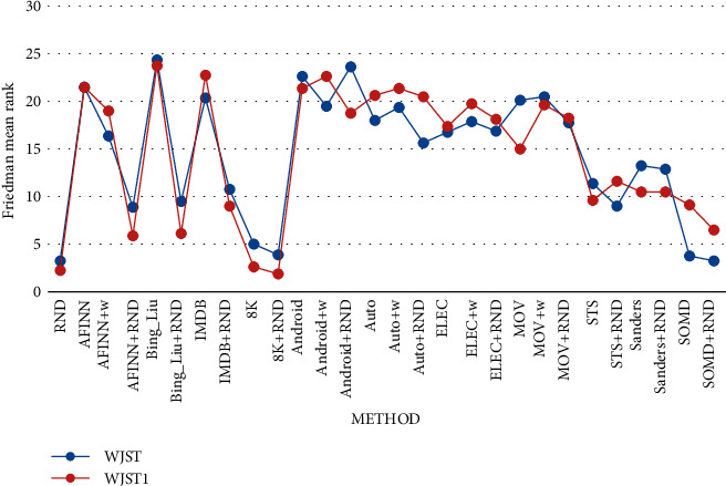
The mean rank according to the Friedman test based on results of Tables 20 and 21.
Figure 12.

Average accuracy values are calculated using different sentiment dictionaries on Android, Automotive, Electronic, Movie, STS, Sanders, and SOMD datasets (based on Tables 20 and 21).
4.6. Evaluation Results According to the Different Number of Topics
In this subsection, the proposed models are examined based on the different topics (5, 10, 15, and 20). The AFINN dictionary is utilized in methods, and the number of distinct windows is three. Evaluations results are shown in Tables 9–12. The proposed methods are better than the baseline methods based on the results. The results show that increasing the number of topics will decrease the perplexity value. WJST1 achieves the highest accuracy on the Movie dataset with 97 percent, but the highest accuracy value on the Movie dataset in WJST is equal to 84 percent. Results show that the proposed methods perform better with different topic number settings, especially for WJST1 with 97% accuracy at |Z| = 5 on the Movie dataset. Based on the results, WJST has a lower perplexity than other methods. WJST1 outperforms WJST and baseline methods in terms of accuracy and topic_coherency. TJST performs better than the WJST method in terms of accuracy, but WJST achieves higher accuracy than JST and other baseline methods. This observation shows that modeling the parameters weight and window improves sentiment classification at the document-level. According to (18), a lower topic_coherency value suggests that the retrieved subjects are of worse quality than one with a highertopic_coherency. The words in a subject accurately describe the subject and have a stronger association with one another.
4.7. Evaluations Results According to the Different Number of Distinct Windows
In this subsection, the proposed models are evaluated according to the different number of separate windows (1, 2, 3, 4, 5, and 6), which are effective for improving the proposed models. In this experiment, the number of topics is five, and the models use the AFINN sentiment dictionary. Based on Table 13, the proposed methods are compared according to accuracy, perplexity, and topic_coherency. The results show that increasing the number of distinct windows will decrease the perplexity value. In the report in Table 13, an increase in the size of a window will reduce the accuracy because it will increase the number of words in the window, and each term may not affect all neighbors in its window.
For instance, as shown in Figure 13, the word terrible has a window size equal to 3. In Table 13, it is assumed that each word affects all neighbors in its window, so Table 13 takes that the unigram terrible effects unigrams film, last, season, sophie, best, and actress. As shown in Figure 13, the word terrible can affect unigrams film, last, and season, but it is not about unigrams sophie, best, and actress. So, finding the words that can be involved in a window is a new challenge that we introduce in this study, and two methods are presented. The first method assumes that each word affects all neighbors in its window, and the second method assumes that each word affects some random neighbors in its window. So, the first method selects all neighbors, but the second method selects some neighbors randomly. In this study, all evaluations are calculated based on the first method, and the second method is considered for the evaluation in Table 14.
Figure 13.

An example for showing the effect of each word on neighbors in its window.
As shown in Table 13, accuracy, perplexity, and topic_coherency values are calculated on Android, Automotive, Electronic, and Movie datasets before random selection using the first method. As shown in Table 14, accuracy, perplexity, and topic_coherency values are calculated on Android, Automotive, Electronic, and Movie datasets after random selection using the second method. So, in Table 13, it is assumed that each word affects all neighbors in its window, but in Table 14, it is assumed that each word affects some random neighbors in its window. As shown in Tables 13 and 14, average values of accuracy, perplexity, and topic_coherency are equal to average values in each column of Tables 13 and 14 for each window size. The values are calculated on Android Automotive, Electronic, and Movie datasets. According to the results, the second method is more stable than the first method in terms of accuracy, but the first method has higher accuracy than the second method. The second method outperforms the first method in terms of perplexity. The first method performs better than the second in terms of accuracy and topic_coherency.
The analysis of the Friedman test on the results of Table 13 demonstrates that there is a statistically significant difference between the performances of the algorithms in terms of accuracy with χ2(5)=27.608 and p < 0.01, in terms of perplexity with χ2(5)=35.143 and p < 0.01, and in terms of topic_coherency with χ2(5)=6.232 and p=0.284. The mean rank of the algorithms based on the Friedman test, which is demonstrated in Figure 14, indicates that (w = 1) outperforms other windows in terms of accuracy. Still, it has lower perplexity and topic_coherency values than other windows. (w = 6) outperforms other windows in perplexity and topic_coherency, but it has a lower accuracy value than other windows. (w = 3) provides a special situation for proposed algorithms in which accuracy, topic_coherency, and perplexity values are between the highest and lowest values (w = 1, 2, 4, 5, and 6). So, in this study, all evaluations are calculated based on (w = 3). The mean rank of the algorithms based on Table 14, which is demonstrated in Figure 15, indicates that (w = 1) ranks first among all the algorithms in Table 14 in terms of accuracy. The analysis of the Friedman test indicates that there is a statistically significant difference in terms of accuracy with χ2(5)=17.550 and p < 0.01, in terms of perplexity with χ2(5)=37.857 and p < 0.01, and in terms of topic_coherency with χ2(5)=5.857 and p=0.320.
Figure 14.

The mean rank of the seven algorithms is in Table 13 according to the Friedman test.
Figure 15.

The mean rank of algorithms is in Table 14 according to the Friedman test.
4.8. Sentiment Classification Using Proposed Methods in Comparison to ALGA
In this subsection, WJST and WJST1 are compared to ALGA [46]. Three datasets have been selected for evaluating the methods. Evaluations results are shown in Figure 16, which compares the results of models with each other according to accuracy, perplexity, and topic_coherency metrics. In ALGA [46], several sentiment lexicons are created for a dataset during the training stage using a genetic algorithm. During the testing process, these dictionaries are employed. Every dictionary has some words and scores. Each chromosome is represented as a vector of sentiment words and their scores in the genetic algorithm employed in the method. The scores are spread between a feeling word's lowest and maximum scores. The primary goal of ALGA is to create a dictionary that reduces errors on training datasets. The sum of scores for words of each instance Ti in dataset Dm using dictionary Lk is calculated using equation (19) and is treated as a feature [46]:
| (19) |
Figure 16.

Sentiment classification on SANDERS, SOMD, and STS datasets, in terms of accuracy (a), perplexity (b), and topic_coherency (c).
Finding the values of words in the dictionaries (chromosomes) and adding them together is how the ALGA value for each instance is calculated. In (19), Wj represents the words of Ti, and vk(Wj) shows the score of Wj in Lk. As mentioned in [46], ALGA will predict a positive instance when the ALGA feature is positive and a negative instance when the ALGA feature is negative. By dividing the number of correct predictions of instances of a given dataset by the total cases, ALGA's accuracy is calculated. In this subsection, proposed methods are compared with ALGA [46] because it can automatically generate a sentiment dictionary. ALGA generates a sentiment dictionary using the genetic algorithm, but proposed methods generate a sentiment dictionary using topic modeling. In proposed models, each document is classified based on P(s| r), the probability of sentiment label given a document. In proposed models, two labels (+, −) are considered, and a document is classified as negative if P(+|r) < P(−|r) and vice versa. Evaluations results can be seen in Figure 16. In this subsection, the number of distinct windows is three, and the number of topics is five. The models use the AFINN sentiment dictionary. According to Figures 16(a)–16(c), each column compares different methods on a dataset. The details of the datasets used in this section are illustrated in Table 4. In this subsection, only the accuracy is considered for the evaluation of ALGA. The ALGA-SW value is achieved by executing ALGA without taking stopwords into account. According to the results, WJST has higher accuracy than TJST on all datasets. WJST1 outperforms WJST and TJST on all datasets. ALGA and ALGA-SW perform better than other methods in terms of accuracy, but WJST1 achieves higher accuracy than ALGA and ALGA-SW on STS and Sanders datasets. The RND method achieves the lowest accuracy value on Sanders and STS datasets. The AFINN + RND method has higher accuracy than the RND method and has a lower accuracy than the AFINN method on Sanders and STS datasets. The RND method outperforms TJST, AFINN, and AFINN + RND methods on the SOMD dataset. In this study, parameters perplexity and topic_coherency are not calculated for ALGA, ALGA-SW, AFINN, RND, and AFINN + RND methods. According to Figure 16, -1 is accuracry1, and -2 is accuracy2.
4.9. Sentiment Classification Using Proposed Methods on Multidomain Datasets
In this subsection, the performance of the proposed methods is compared with baseline methods on a multidomain dataset. In this experiment, the number of distinct windows and topics is three and five, respectively, and the models use the AFINN sentiment dictionary. The multidomain dataset contains reviews taken from multiple domains (product types). The details of the multidomain dataset used in this section are illustrated in Table 22.
Table 22.
Description of the multidomain dataset used in this section.
| # | Domains | Number of reviews | Vocabulary size | Number of words |
|---|---|---|---|---|
| 1 | Android, Automotive, Electronic, and Movie | 1600 | 11183 | 100113 |
As shown in Figure 17, accuracy, perplexity, and topic_coherency values are calculated on a multidomain dataset that contains Android. Automotive, Electronic, and Movie domains. The methods WJST-dictionary and WJST1-dictionary classify each document according to P(s|r)=Ns,r/Nr. The word sentiment label is directly obtained from WJST and WJST1 lexicons achieved by WJST and WJST1 on the multidomain dataset. According to Figure 17, -1 is accuracry1 and -2 is accuracy2. Based on the results, WJST has a lower perplexity value than other methods. WJST1 outperforms WJST in terms of topic_coherency. WJST performs better than the WJST1 method in terms of accuracy because the distributions θ, ξ, and ψ in WJST depend on document, but in WJST1, the distributions θ, ξ, and ψ do not depend on the document. Dependency between documents of a domain is more than documents in different domains. A pattern in the documents of a domain may not exist in the documents of other domains. Therefore, calculations on multidomain datasets should be local and not cover all domains. For example, considering the distributions P(z| s) and P(z| s, r), where z is topic, s is the sentiment, and r is documents. In the first state (P(z| s)), the topic depends on sentiment, and the distribution covers all documents in different domains. Perhaps a topic was positive in one domain and negative in another. Therefore, it is better to depend the topic on the documents of a domain, not all domains. Thus, the topic is limited to the document (and domain), and contradiction between different domains is eliminated. Therefore, WJST is suitable for multidomain datasets, and WJST1 is a version of WJST suitable for single-domain datasets. Sentiment classification on multidomain datasets is a challenge, and our solution in this study is using WJST, whose distributions (θ, ξ, and ψ) depend on the document. Sentiment classification on multidomain datasets is a challenge, and further studies can be conducted to investigate this problem for future research.
Figure 17.

Sentiment classification values are calculated on a multidomain dataset in terms of accuracy (a), perplexity (b), and topic_coherency (c).
4.10. Comparison with Other Methods
In this subsection, the best performance of the proposed methods is compared with 57 competitors [13, 76]; [82–88], [8–10, 46] which is shown in Table 23. The details of the datasets used in this section are illustrated in Table 4.
Table 23.
Sentiment classification on MR, Sanders, SOMD, STS, Amazon, IMDB, and Yelp datasets.
| Method/dataset | MR | Sanders | SOMD | STS | Amazon | IMDB | Yelp |
|---|---|---|---|---|---|---|---|
| ALGA [46] | — | 0.8067 | 0.8147 | 0.7668 | — | — | — |
| ALGA-SW [46] | — | 0.7868 | 0.7877 | 0.7886 | — | — | — |
| BPSO (Shang et al., 2016) | — | — | — | — | 0.7439 | 0.79 | 0.789 |
| BICA (Mirhosseini et al., 2017) | — | — | — | — | 0.793 | 0.745 | 0.763 |
| BABC (Schiezaro et al., 2013) | — | — | — | — | 0.7509 | 0.74 | 0.736 |
| MaxEnt (Saif et al., 2014) | — | 0.8362 | — | 0.7782 | — | — | — |
| NB (Saif et al., 2014) | — | 0.8266 | — | 0.8106 | — | — | — |
| LS-all [13] | — | 0.8199 | — | — | — | — | — |
| SVM-all [13] | — | 0.8214 | — | — | — | — | — |
| RMTL [13] | — | 0.827875 | — | — | — | — | — |
| MTL-graph [13] | — | 0.801725 | — | — | — | — | — |
| CMSC [13] | — | 0.846325 | — | — | — | — | — |
| LSTM-all [13] | — | 0.8063 | — | — | — | — | — |
| MTL-CNN [13] | — | 0.829825 | — | — | — | — | — |
| MTL-DNN [13] | — | 0.817 | — | — | — | — | — |
| ASP-MTL [13] | — | 0.85125 | — | — | — | — | — |
| NeuroSent [13] | — | 0.834575 | — | — | — | — | — |
| DAM [13] | — | 0.863225 | — | — | — | — | — |
| SVM-BoW (Da Silva et al., 2014) | — | 0.8243 | 0.7402 | — | — | — | — |
| SVM-BoW + lex (Da Silva et al., 2014) | — | 0.8398 | 0.7893 | — | — | — | — |
| RF-BoW (Da Silva et al., 2014) | — | 0.7924 | 0.7391 | — | — | — | — |
| RF-BoW + lex (Da Silva et al., 2014) | — | 0.8235 | 0.7936 | — | — | — | — |
| LR-BoW (Da Silva et al., 2014) | — | 0.7745 | 0.7238 | — | — | — | — |
| LR-BoW + lex (Da Silva et al., 2014) | — | 0.7949 | 0.7806 | — | — | — | — |
| MNB-BoW (Da Silva et al., 2014) | — | 0.7982 | 0.7543 | — | — | — | — |
| MNB-BoW + lex (Da Silva et al., 2014) | — | 0.8341 | 0.8013 | — | — | — | — |
| ENS(LR + RF + MNB)-BoW (Da Silva et al., 2014) | — | 0.8276 | 0.7555 | — | — | — | — |
| ENS(LR + RF + MNB)-BoW + lex (Da Silva et al., 2014) | — | 0.8489 | 0.8035 | — | — | — | — |
| SVM-FH (Da Silva et al., 2014) | — | 0.4975 | 0.5131 | — | — | — | — |
| SVM-FH + lex (Da Silva et al., 2014) | — | 0.7500 | 0.6299 | — | — | — | — |
| RF-FH (Da Silva et al., 2014) | — | 0.5564 | 0.6136 | — | — | — | — |
| RF-FH + lex (Da Silva et al., 2014) | — | 0.7163 | 0.7260 | — | — | — | — |
| LR-FH (Da Silva et al., 2014) | — | 0.5694 | 0.6529 | — | — | — | — |
| LR-FH + lex (Da Silva et al., 2014) | — | 0.7598 | 0.7303 | — | — | — | — |
| MNB-FH (Da Silva et al., 2014) | — | 0.5425 | 0.6070 | — | — | — | — |
| MNB-FH + lex (Da Silva et al., 2014) | — | 0.7508 | 0.7139 | — | — | — | — |
| ENS(LR + RF + MNB)-FH (Da Silva et al., 2014) | — | 0.5784 | 0.6517 | — | — | — | — |
| ENS(LR + RF + MNB)-FH + lex (Da Silva et al., 2014) | — | 0.7663 | 0.7456 | — | — | — | — |
| WS-TSWE' [76] | 0.841 | — | — | — | — | — | — |
| WS-TSWE [76] | 0.824 | — | — | — | — | — | — |
| TSWE-P [76] | 0.726 | — | — | — | — | — | — |
| TSWE + P [76] | 0.782 | — | — | — | — | — | — |
| JSTH [76] | 0.681 | — | — | — | — | — | — |
| HTSM [76] | 0.796 | — | — | — | — | — | — |
| SAE (Pagliardini et al., 2018) | 0.861 | — | — | — | — | — | — |
| ParagraphVec DBOW (Pagliardini et al., 2018) | 0.763 | — | — | — | — | — | — |
| ParagraphVec DM (Pagliardini et al., 2018) | 0.764 | — | — | — | — | — | — |
| IST (Pu et al., 2019) | 0.827 | — | — | — | — | — | — |
| UST (Pu et al., 2019) | 0.832 | — | — | — | — | — | — |
| UIST (Pu et al., 2019) | 0.845 | — | — | — | — | — | — |
| RND | 0.4895 | 0.4852 | 0.4847 | 0.5346 | 0.491 | 0.498 | 0.506 |
| AFINN | 0.601 | 0.674 | 0.3395 | 0.734 | 0.731 | 0.698 | 0.689 |
| AFINN + RND | 0.5455 | 0.5424 | 0.4475 | 0.6038 | 0.574 | 0.575 | 0.559 |
| JST [8] | 0.613 | 0.6176 | 0.4934 | 0.6398 | 0.611 | 0.605 | 0.579 |
| TJST [8] | 0.62 | 0.5898 | 0.4639 | 0.6814 | 0.645 | 0.616 | 0.614 |
| RJST [12] | 0.51 | 0.6086 | 0.4967 | 0.6232 | 0.609 | 0.546 | 0.561 |
| TS [9] | 0.5 | 0.5612 | 0.5251 | 0.565 | 0.54 | 0.545 | 0.547 |
| WJST-1 | 0.821 | 0.7268 | .75786 | 0.7126 | 0.779 | 0.76 | 0.737 |
| WJST-2 | 0.818 | 0.7203 | 0.75775 | 0.7181 | 0.829 | 0.761 | 0.726 |
| WJST1-1 | 0.8445 | 0.832 | 0.8 | 0.8317 | 0.796 | 0.77 | 0.773 |
| WJST1-2 | 0.843 | 0.8352 | 0.7859 | 0.8373 | 0.798 | 0.774 | 0.769 |
4.11. Comparison with Discriminative Models
The proposed methods are compared to baseline approaches such as logistic regression and SVM on four datasets in the following experiment. The multidomain dataset contains Android, Automotive, Electronic, and Movie domains. As shown in Table 24, the accuracy value is calculated on four datasets. The results demonstrate that proposed methods have improved notably over AFINN and the baseline methods on all datasets. Based on Table 24, methods use two systems in preprocessing phase, which includes Bag of Word (BOW) and Term Frequency Inverse Document Frequency (TF-IDF). In the BOW system, more word frequency reflects more importance of the word. TF-IDF system believes that high frequency may not be able to provide much information. Furthermore, rare words contribute more weight to the method. According to evaluation results, the results of the TF-IDF system are better than the BOW system.
Table 24.
Sentiment classification in comparison with discriminative models on different datasets.
| Method\Dataset | Android | Automotive | Electronic | Movie | |
|---|---|---|---|---|---|
| RND | 0.48 | 0.4925 | 0.465 | 0.525 | |
| AFINN | 0.6975 | 0.625 | 0.675 | 0.595 | |
| RND + AFINN | 0.58 | 0.535 | 0.52 | 0.555 | |
| LOGISTIC REGRESSION(BOW) | 0.53 | 0.52 | 0.5338 | 0.57 | |
| RANDOMFOREST(BOW) | 0.69 | 0.65 | 0.60 | 0.6575 | |
| SVM(BOW) | 0.49 | 0.51 | 0.54 | 0.5675 | |
| DECISIONTREE(BOW) | 0.71 | 0.70 | 0.56 | 0.665 | |
| NAIVE_BAYES(BOW) | 0.51 | 0.55 | 0.4712 | 0.555 | |
| KNEIGHBORS (N = 3, BOW) | 0.55 | 0.57 | 0.55 | 0.5725 | |
| KNEIGHBORS (N = 4,BOW) | 0.56 | 0.575 | 0.5915 | 0.585 | |
| KNEIGHBORS (N = 5,BOW) | 0.57 | 0.5725 | 0.55 | 0.59 | |
| KNEIGHBORS (N = 6,BOW) | 0.57 | 0.5675 | 0.56 | 0.61 | |
| LOGISTIC REGRESSION (TF-IDF) | 0.61 | 0.63 | 0.83 | 0.59 | |
| RANDOMFOREST (TF-IDF) | 0.575 | 0.6 | 0.7243 | 0.5225 | |
| SVM (TF-IDF) | 0.5825 | 0.59 | 0.80 | 0.54 | |
| DECISIONTREE (TF-IDF) | 0.55 | 0.57 | 0.7043 | 0.55 | |
| NAIVE_BAYES (TF-IDF) | 0.58 | 0.60 | 0.7945 | 0.58 | |
| KNEIGHBORS (N = 3, TF-IDF) | 0.65 | 0.63 | 0.53 | 0.7125 | |
| KNEIGHBORS (N = 4, TF-IDF) | 0.65 | 0.63 | 0.56 | 0.7125 | |
| KNEIGHBORS (N = 5, TF-IDF) | 0.65 | 0.63 | 0.51 | 0.7125 | |
| KNEIGHBORS (N = 6, TF-IDF) | 0.65 | 0.5725 | 0.53 | 0.7125 | |
| JST | 0.625 | 0.6575 | 0.7025 | 0.7575 | |
| ASUM | 0.613 | 0.6322 | 0.71 | 0.772 | |
| TJST | 0.765 | 0.7675 | 0.76 | 0.9475 | |
| RJST | 0.5825 | 0.615 | 0.5525 | 0.62 | |
| TS | 0.5425 | 0.5525 | 0.5475 | 0.5425 | |
| WJST | Accuracy1 | 0.795 | 0.755 | 0.8625 | 0.8475 |
| Accuracy2 | 0.7825 | 0.7475 | 0.875 | 0.8325 | |
| WJST1 | Accuracy1 | 0.865 | 0.8 | 0.8475 | 0.97 |
| Accuracy2 | 0.8525 | 0.795 | 0.855 | 0.9675 | |
4.12. Comparison with JST According to Extended Features
Suppose a unigram corresponds to the sentiment lexicon. In that case, its polarity will be equal to the subjectivity of the lexicon in order to identify the emotion label of the unigram for trying to prepare prior emotion information. The following technique is used to decide the emotion label of a bigram to prepare prior emotion information: If words of the bigram have the same polarity, the bigram's polarity will be the same as that of the words. If one of the words is in the lexicon, the bigram's polarity will equal the lexicon's subjectivity. The bigram's polarity will be opposed to the polarity of the second word if the first word is ‘not.' The following methodology is used to decide the emotion label of a trigram in order to prepare prior emotion information. If words of the trigram have the same polarity, the trigram's polarity will be the same as that of the words. If one of them is in the lexicon, the trigram's polarity will equal the lexicon's subjectivity. The trigram's polarity will be opposed to the second or third word's polarity if the first or second word is ‘not.' The proposed methods are compared with JST on four datasets (single-domain) according to extended features (bigrams and trigrams) in the following experiment.
As shown in Table 25, the accuracy value is calculated on four datasets, and the experiment extends the features to bigrams and trigrams. According to the results, WJST1 outperforms WJST. According to evaluations results, proposed models outperform JST because the additional parameters can influence the process of producing words in a review appropriately. The perplexity value varies on different datasets because the size of datasets is different. As the number of grams increases, perplexity is increased because in each document, in addition to the unigrams (+bigrams), bigrams (+trigrams) are added to the data, and the size of the dataset is increased. As the number of grams increases, accuracy is improved. In some cases, it gets worse because higher grams (bigram or trigrams) are sometimes meaningless.
Table 25.
Sentiment classification according to extended features (bigrams and trigrams) on different datasets (single-domain).
| Model | Gram | Metric\dataset | Android | Automotive | Electronic | Movie |
|---|---|---|---|---|---|---|
| JST | U ∗ | Accuracy | 0.625 | 0.6275 | 0.675 | 0.7575 |
| Perplexity | 19.6726 | 24.7154 | 25.227 | 27.3111 | ||
| Topic_Coh | −4.6026 | −1.486 | −1.5892 | −1.0123 | ||
| U + B∗ | Accuracy | 0.655 | 0.7025 | 0.75 | 0.835 | |
| Perplexity | 66.1882 | 86.6897 | 81.3375 | 98.9201 | ||
| Topic_Coh | −2.4595 | −1.0417 | −0.9823 | −0.4165 | ||
| U + B + T∗ | Accuracy | 0.6775 | 0.5825 | 0.7525 | 0.7275 | |
| Perplexity | 114.8812 | 158.7113 | 156.1383 | 190.8403 | ||
| Topic_Coh | −1.5776 | −2.3915 | −0.7030 | −0.1288 | ||
|
| ||||||
| WJST | U | Accuracy1 | 0.7925 | 0.755 | 0.8625 | 0.7225 |
| Accuracy2 | 0.7775 | 0.7475 | 0.875 | 0.71 | ||
| Perplexity | 16.7303 | 21.2008 | 20.5489 | 23.1145 | ||
| Topic_Coh | −0.5547 | −1.6542 | −2.0442 | −0.0751 | ||
| U + B | Accuracy1 | 0.6825 | 0.63 | 0.67 | 0.65 | |
| Accuracy2 | 0.68 | 0.625 | 0.6675 | 0.6475 | ||
| Perplexity | 36.5505 | 49.8584 | 48.2008 | 58.0838 | ||
| Topic_Coh | −1.3976 | −4.0214 | −1.2513 | −0.0423 | ||
| U + B + T | Accuracy1 | 0.7325 | 0.6825 | 0.635 | 0.6475 | |
| Accuracy2 | 0.7325 | 0.6825 | 0.615 | 0.6325 | ||
| Perplexity | 52.9205 | 72.7629 | 76.2545 | 88.1860 | ||
| Topic_Coh | −1.3242 | −1.5525 | −1.2409 | −2.5170 | ||
|
| ||||||
| WJST1 | U | Accuracy1 | 0.81 | 0.80 | 0.79 | 0.97 |
| Accuracy2 | 0.7925 | 0.79 | 0.80 | 0.9625 | ||
| Perplexity | 16.6787 | 21.4357 | 22.6012 | 24.6302 | ||
| Topic_Coh | −0.187 | −1.1883 | −1.1683 | −0.1348 | ||
| U + B | Accuracy1 | 0.7 | 0.7625 | 0.8575 | 0.935 | |
| Accuracy2 | 0.7 | 0.7625 | 0.8525 | 0.935 | ||
| Perplexity | 38.5603 | 49.5167 | 54.7041 | 62.3459 | ||
| Topic_Coh | −2.0962 | −1.8607 | −0.9744 | −0.0617 | ||
| U + B + T | Accuracy1 | 0.83 | 0.7625 | 0.745 | 0.9475 | |
| Accuracy2 | 0.8275 | 0.7675 | 0.745 | 0.9475 | ||
| Perplexity | 55.5819 | 75.3624 | 77.6660 | 96.3675 | ||
| Topic_Coh | −1.3837 | −0.1840 | −0.9334 | −0.0333 | ||
U∗: unigram. B∗: bigram. T∗: trigram.
4.13. Discussions on the Limitations of the Proposed Methods
Although the analysis of the results of the evaluation can demonstrate the best performance of proposed methods, proposed methods have some limitations, as follows:
The first limitation is the time complexity of the proposed methods (O(G·wALL·|S|·|Z|·|Q|·|E|)) which is more than baseline methods (O(G·wALL·|S|·|Z|)) according to Table 3 in Section 3.3.
The second limitation is the window size. On the report in Table 13, an increase in the size of a window will decrease the accuracy because it will increase the number of words in the window, and each term may not affect all neighbors in its window. Therefore, finding the words that can be involved in a window is a new challenge that we introduce in this study, and two methods are presented in Section 4.7. The first method assumes that each word affects all neighbors in its window, and the second method assumes that each word affects some random neighbors in its window.Therefore, the first method selects all neighbors, but the second method selects some neighbors randomly. According to the results, the second method is more stable than the first method in terms of accuracy, but the first method has a higher accuracy value than the second method. The second method outperforms the first method in terms of perplexity. The first method performs better than the second in terms of accuracy and topic_coherency.
4.14. A Concise Description of the Proposed Solutions and the Results
The main problem in this study is to examine a user's opinion about a product or movie, for example. This means identifying whether a user has a positive or negative idea about a subject (a product or movie).
Two novel models have been proposed that use topic modeling to solve the above problem. So, our solution is using a technique named topic modeling. Proposed models extend and improve JST (as a topic model) through two new parameters. To improve JST, proposed models consider the effect of words on each other. The new parameters have an immense effect on model accuracy regarding evaluation results. According to evaluations results, the proposed models outperform JST because the additional parameters can influence the process of producing words in a review appropriately. They can improve sentiment classification at the document-level. Also, in the evaluation results report, proposed methods are more accurate than discriminative models such as SVM and logistic regression. Proposed methods are more flexible than discriminative models because other information, such as the top 10 words, can be extracted from the heart of the data.
5. Conclusion
In this study, two new models called WJST and WJST1 have been presented that extend JST and improve accuracy metrics. Reviewing the various articles about sentiment analysis indicates that the proposed models are associated with innovation and lead to remarkable results compared to the baseline methods. The proposed models can generate a sentiment dictionary. According to evaluations results, the proposed models consider the effect of words on each other using the extra parameters, which are important and influential. The evaluation results indicate that the accuracy has been improved compared to the baseline methods such as JST, RJST, TS, TJST, and ALGA. Results show that the proposed methods perform better with different topic number settings. WJST1 outperforms other methods in terms of accuracy, demonstrating its effectiveness of that. Prior sentiment information affects perplexity and topic_coherency lower than accuracy.
According to evaluations results, using the AFINN dictionary as prior sentiment information is more effective than using the NO_AFINN state. ALGA uses the genetic algorithm to generate a sentiment dictionary; however, proposed methods use topic modeling to generate this dictionary. According to the evaluation results, the proposed models outperform JST because the additional parameters could influence the process of producing words in a review appropriately. They have the potential to increase the emotion detection's accuracy at the level of the document. The proposed methods are unsupervised, and no labeled data is required. Proposed methods can automatically assess web comments and categorize reviews as positive or negative. The proposed methods have tried to increase the accuracy with fewer parameters and, at the same time, simplicity compared to the existing methods. The proposed methods both analyze emotions at the document-level and create an emotional dictionary. They are also the first methods to create an emotional dictionary through a topic modeling technique and in an automatic and accurate way. The proposed methods are the first methods that consider the words in the text and their effect on each other in a dynamic and weighty way. Also, they are parametric.
6. Future Work
The proposed models are parametric in the present study, and further studies will be conducted to investigate nonparametric models. Sentiment classification on multidomain datasets is a challenge, and further studies can be conducted to investigate this problem for future research. In future research, the proposed methods can be evaluated on more datasets. More parameters can also be assessed. Twitter social network data have obtained significant attention in natural language processing studies, with certain conditions, such as short data length. In future articles, the proposed methods can be modified to analyze emotions with specific Twitter data.
Data Availability
The datasets used during the current study are available from the corresponding author (a.osmani@qiau.ac.ir) upon reasonable request.
Conflicts of Interest
The authors declare that they have no conflicts of interest.
References
- 1.Peikari N., Yaghobi A., Taheri R. Analysis of Emotions on the Twitter Social Network with the Text-Mining Technique . Iran: International Conference on Web Research; 2015. [Google Scholar]
- 2.Zhang L., Liu B. Sentiment analysis and opinion mining. In: Sammut C., Webb G. I., editors. Encyclopedia of Machine Learning and Data Mining . Illinois Chicago: Springer; 2017. [DOI] [Google Scholar]
- 3.Pang B., Lee L. A sentimental education: sentiment analysis using subjectivity summarization based on minimum cuts. Proceedings of the 42nd Annual Meeting on Association for Computational Linguistics; July 2004; Barcelona Spain. ACL; pp. 271–278. [Google Scholar]
- 4.Pang B., Lee L. Opinion mining and sentiment analysis. Foundations and Trends in Information Retrieval . 2008;2(1–2):1–135. doi: 10.1561/1500000011. [DOI] [Google Scholar]
- 5.Medhat W., Hassan A., Korashy H. Sentiment analysis algorithms and applications: a survey. Ain Shams Engineering Journal . 2014;5(4):1093–1113. doi: 10.1016/j.asej.2014.04.011. [DOI] [Google Scholar]
- 6.Chen Z., Liu B. Lifelong Machine Learning . San Rafael, California USA: Morgan & Claypool Publishers; 2018. [Google Scholar]
- 7.Griffiths T. L., Steyvers M. Finding scientific topics. Proceedings of the National Academy of Sciences . 2004;101(suppl_1):5228–5235. doi: 10.1073/pnas.0307752101. [DOI] [PMC free article] [PubMed] [Google Scholar]
- 8.Lin C., He Y. Joint sentiment/topic model for sentiment analysis. Proceedings of the 18th ACM conference on Information and knowledge management, ACM; November 2009; New York, NY, USA. pp. 375–384. [DOI] [Google Scholar]
- 9.Dermouche M., Kouas L., Velcin J., Loudcher S. A joint model for topic-sentiment modeling from text. Proceedings of the 30th Annual ACM Symposium On Applied Computing, ACM; April 2015; New York, NY, USA. pp. 819–824. [DOI] [Google Scholar]
- 10.Lin C., He Y., Everson R., Ruger S. Weakly supervised joint sentiment-topic detection from text. IEEE Transactions on Knowledge and Data Engineering . 2012;24:1134–1145. doi: 10.1109/tkde.2011.48. [DOI] [Google Scholar]
- 11.Liu B. Sentiment analysis and opinion mining. Synthesis Lectures on Human Language Technologies . 2012;5(1):1–167. doi: 10.2200/s00416ed1v01y201204hlt016. [DOI] [Google Scholar]
- 12.Liu B., Zhang L. A survey of opinion mining and sentiment analysis. In: Aggarwal C., Zhai C., editors. Mining Text Data . Boston, MA: Springer; 2012. [DOI] [Google Scholar]
- 13.Yuan Z., Wu S., Wu F., Liu J., Huang Y. Domain attention model for multi-domain sentiment classification. Knowledge-Based Systems . 2018;155:1–10. doi: 10.1016/j.knosys.2018.05.004. [DOI] [Google Scholar]
- 14.Blei D. M., Ng A. Y., Jordan M. I. Latent dirichlet allocation. Journal of Machine Learning Research . 2003;3:993–1022. [Google Scholar]
- 15.Li X., Zhang A., Li C., Guo L., Wang W., Ouyang J. Relational biterm topic model: short-text topic modeling using word embeddings. The Computer Journal . 2018;62(3):359–372. doi: 10.1093/comjnl/bxy037. [DOI] [Google Scholar]
- 16.Yang M., Chen X., Tu W., Lu Z., Zhu J., Qu Q. A topic drift model for authorship attribution. Neurocomputing . 2018;273:133–140. doi: 10.1016/j.neucom.2017.08.022. [DOI] [Google Scholar]
- 17.Chien J.-T., Lee C.-H., Tan Z.-H. Latent Dirichlet mixture model. Neurocomputing . 2018;278:12–22. doi: 10.1016/j.neucom.2017.08.029. [DOI] [Google Scholar]
- 18.Osmani A., Mohasefi JB., Gharehchopogh FS. Enriched latent dirichlet allocation for sentiment analysis. Expert Systems . 2020;37 doi: 10.1111/exsy.12527.e12527 [DOI] [Google Scholar]
- 19.Lin C., Ibeke E., Wyner A., Guerin F. Sentiment-topic modeling in text mining. Wiley Interdisciplinary Reviews: Data Mining and Knowledge Discovery . 2015;5(5):246–254. doi: 10.1002/widm.1161. [DOI] [Google Scholar]
- 20.Jo Y., Oh A. H. Aspect and sentiment unification model for online review analysis. ACM ; Proceedings of the Fourth ACM International Conference on Web Search and Data Mining; February 2011; Hong Kong, China. pp. 815–824. [DOI] [Google Scholar]
- 21.Wahid J. A., Shi L., Gao Y., et al. Topic2features: a novel framework to classify noisy and sparse textual data using LDA topic distributions. PeerJ Computer Science . 2021;7:p. e677. doi: 10.7717/peerj-cs.677. [DOI] [PMC free article] [PubMed] [Google Scholar]
- 22.Zhou Y., Liao L., Gao Y., Wang R., Huang H. TopicBERT: a topic-enhanced neural language model fine-tuned for sentiment classification. Proceedings of the IEEE Transactions on Neural Networks and Learning Systems; August 2021; New York, NY, USA. [DOI] [PubMed] [Google Scholar]
- 23.Abdi S., Bagherzadeh J., Gholami G., Tajbakhsh M. S. Using an auxiliary dataset to improve emotion estimation in users’ opinions. Journal of Intelligent Information Systems . 2021;56(3):581–603. doi: 10.1007/s10844-021-00643-y. [DOI] [Google Scholar]
- 24.Alam M. H., Ryu W.-J., Lee S. Joint multi-grain topic sentiment: modeling semantic aspects for online reviews. Information Sciences . 2016;339:206–223. doi: 10.1016/j.ins.2016.01.013. [DOI] [Google Scholar]
- 25.Hua T., Lu C.-T., Choo J., Reddy C. K. Probabilistic topic modeling for comparative analysis of document collections. ACM Transactions on Knowledge Discovery from Data . 2020;14(2):1–27. doi: 10.1145/3369873. [DOI] [Google Scholar]
- 26.Rao Y., Li Q., Mao X., Wenyin L. Sentiment topic models for social emotion mining. Information Sciences . 2014;266:90–100. doi: 10.1016/j.ins.2013.12.059. [DOI] [Google Scholar]
- 27.Mahadevan A., Arock M. Integrated topic modeling and sentiment analysis: a review rating prediction approach for recommender systems. Turkish Journal of Electrical Engineering and Computer Sciences . 2020;28(1):107–123. doi: 10.3906/elk-1905-114. [DOI] [Google Scholar]
- 28.Xia Y., Tang G., Zhao H., Cambria E., Zheng T.-F. Using word sense as a latent variable in LDA can improve topic modeling. Proceedings of the 6th International Conference on Agents and Artificial Intelligence; January 2014; Loire Valley France. Science and Technology Publications; pp. 532–537. [Google Scholar]
- 29.Meng Y., Speier W. F., Ong M., Arnold C. HCET: hierarchical clinical embedding with topic modeling on electronic Health Record for predicting depression. IEEE Journal of Biomedical and Health Informatics . 2020;25(4):1–8. doi: 10.1109/JBHI.2020.3004072. [DOI] [PMC free article] [PubMed] [Google Scholar]
- 30.Qiang J., Qian Z., Li Y., Yuan Y., Wu X. Short text topic modeling techniques, applications, and performance: a survey. IEEE Transactions on Knowledge and Data Engineering . 2020;34:1–19. [Google Scholar]
- 31.Yang Q., Rao Y., Xie H., Wang J., Wang F. L., Chan W. H. Segment-level joint topic-sentiment model for online review analysis. IEEE Intelligent Systems . 2019;34(1):43–50. doi: 10.1109/mis.2019.2899142. [DOI] [Google Scholar]
- 32.Vayansky I., Kumar S. A. P. A review of topic modeling methods. Information Systems . 2020;94:1–32. doi: 10.1016/j.is.2020.101582. [DOI] [Google Scholar]
- 33.Bigne E., Ruiz C., Cuenca A., Perez C., Garcia A. What drives the helpfulness of online reviews? A deep learning study of sentiment analysis, pictorial content and reviewer expertise for mature destinations. Journal of Destination Marketing & Management . 2021;20 doi: 10.1016/j.jdmm.2021.100570. [DOI] [Google Scholar]
- 34.Safder Q., Mahmood Z., Sarwar R., et al. Sentiment analysis for Urdu online reviews using deep learning models. Expert Systems . 2021 doi: 10.1111/exsy.12751. [DOI] [Google Scholar]
- 35.Pathak AR., Pandey M., Rautaray S. Topic-level sentiment analysis of social media data using deep learning. Applied Soft Computing . 2021;108 doi: 10.1016/j.asoc.2021.107440. [DOI] [Google Scholar]
- 36.Feng S., Zhou H., Dong H. Using deep neural network with small dataset to predict material defects. Materials & Design . 2019;162:300–310. doi: 10.1016/j.matdes.2018.11.060. [DOI] [Google Scholar]
- 37.Khezri S., Faez K., Osmani A. Modified discrete binary PSO based sensor placement in WSN networks. Proceedings of the 2010 International Conference on Computational Intelligence and Communication Networks; November 2010; Bhopal, India. pp. 200–204. [Google Scholar]
- 38.Khezri S., Meybodi M. R., Osmani A. Fuzzy adaptive PBIL based sensor placement in wireless sensor networks. Proceedings of the 2011 International Symposium on Computer Networks and Distributed Systems; February 2011a; Tehran, Iran. CNDS); pp. 216–221. [DOI] [Google Scholar]
- 39.Khezri S., Faez K., Osmani A. An intelligent sensor placement method to reach a high coverage in wireless sensor networks. International Journal of Grid and High Performance Computing . 2011b;3(3):54–68. doi: 10.4018/jghpc.2011070105. [DOI] [Google Scholar]
- 40.Gharehchopogh F. S., Gholizadeh H. A comprehensive survey: whale Optimization Algorithm and its applications. Swarm and Evolutionary Computation . 2019;48:1–24. doi: 10.1016/j.swevo.2019.03.004. [DOI] [Google Scholar]
- 41.Abdollahzadeh B., Gharehchopogh F. S., Mirjalili S. African vultures optimization algorithm: a new nature-inspired metaheuristic algorithm for global optimization problems. Computers & Industrial Engineering . 2021a;158 doi: 10.1016/j.cie.2021.107408. [DOI] [Google Scholar]
- 42.Abdollahzadeh B., Soleimanian Gharehchopogh F., Mirjalili S. Artificial gorilla troops optimizer: a new nature‐inspired metaheuristic algorithm for global optimization problems. International Journal of Intelligent Systems . 2021b;36(10):5887–5958. doi: 10.1002/int.22535. [DOI] [Google Scholar]
- 43.Asghari K., Masdari M., Gharehchopogh F. S., Saneifard R. Multi-swarm and chaotic whale-particle swarm optimization algorithm with a selection method based on roulette wheel. Expert Systems . 2021;38(8) doi: 10.1111/exsy.12779. [DOI] [Google Scholar]
- 44.Asgarnezhad R., Monadjemi S. A., Soltanaghaei M. An application of MOGW optimization for feature selection in text classification. The Journal of Supercomputing . 2021;77(6):5806–5839. doi: 10.1007/s11227-020-03490-w. [DOI] [Google Scholar]
- 45.Abasi A. K., Khader A. T., Al-Betar M. A., Naim S., Makhadmeh S. N., Alyasseri Z. A. A. An improved text feature selection for clustering using binary grey wolf optimizer. In: Zain Z., editor. Proceedings of the 11th National Technical Seminar on Unmanned System Technology 2019. Lecture Notes in Electrical Engineering . Vol. 666. Singapore: Springer; 2021. [DOI] [Google Scholar]
- 46.Osmani A., Mohasefi J. B., Gharehchopogh F. S. Sentiment classification using two effective optimization methods derived from the artificial bee colony optimization and imperialist competitive algorithm. The Computer Journal . 2022;65(1):18–66. doi: 10.1093/comjnl/bxz163. [DOI] [Google Scholar]
- 47.Tang M., Jin J., Liu Y., Li C., Zhang W. Integrating topic. Sentiment. And syntax for modeling online reviews: a topic model approach. ASME. J. Comput. Inf. Sci. Eng . 2018;19(1):1–12. doi: 10.1115/1.4041475. [DOI] [Google Scholar]
- 48.Gong L., Wang H. When sentiment analysis meets social network: a holistic user behavior modeling in opinionated data. Proceedings of the 24th acm sigkdd international conference on knowledge discovery & data mining (kdd ’18); July 2018; London, United Kingdom. Association for Computing Machinery (ACM); pp. 1455–1464. [DOI] [Google Scholar]
- 49.Cheng K., Li J., Tang J., Liu H. Unsupervised Sentiment Analysis with Signed Social Networks. Proceedings of the AAAI Conference on Artificial Intelligence, 31(1), Association for the Advancement of Artificial Intelligence (AAAI Press); 2017; San Francisco, California, USA. pp. 3429–3435. [Google Scholar]
- 50.Iqbal M., Karim A., Kamiran F. Balancing prediction errors for robust sentiment classification. ACM Transactions on Knowledge Discovery from Data . 2019;13(3):1–21. doi: 10.1145/3328795. [DOI] [Google Scholar]
- 51.Ibrahim Hussein M., Kang X., Feng L., Ibrahim Z., Waheed Ahmed A., Guilin Q. A cross-lingual sentiment topic model evolution over time. A Cross-lingual Sentiment Topic Model Evolution over Time. Intelligent Data Analysis . 2020;24(2):253–266. [Google Scholar]
- 52.Kumar S., Singh R., Khan M. Z., Noorwali A. Design of adaptive ensemble classifier for online sentiment analysis and opinion mining. PeerJ Computer Science . 2021;7 doi: 10.7717/peerj-cs.660. [DOI] [PMC free article] [PubMed] [Google Scholar]
- 53.Keshavarz H., Abadeh M. S. ALGA: adaptive lexicon learning using genetic algorithm for sentiment analysis of microblogs. Knowledge-Based Systems . 2017;122:1–16. doi: 10.1016/j.knosys.2017.01.028. [DOI] [Google Scholar]
- 54.Kalarani P., Selva Brunda S. Sentiment analysis by POS and joint sentiment topic features using SVM and ANN. Soft Computing . 2019;23(16):7067–7079. doi: 10.1007/s00500-018-3349-9. [DOI] [Google Scholar]
- 55.Farkhod A., Abdusalomov A., Makhmudov F., Cho Y. I. LDA-based topic modeling sentiment analysis using topic/document/sentence (TDS) model. Applied Sciences . 2021;11(23):p. 11091. doi: 10.3390/app112311091. [DOI] [Google Scholar]
- 56.Fatemi M., Safayani M. Joint sentiment/topic modeling on text data using a boosted restricted Boltzmann Machine. Multimedia Tools and Applications . 2019;78(15):20637–20653. doi: 10.1007/s11042-019-7427-5. [DOI] [Google Scholar]
- 57.Liang Q., Ranganathan S., Wang K., Deng X. JST-RR model: joint modeling of ratings and reviews in sentiment-topic prediction. 2021. https://arxiv.org/abs/2102.11048 .
- 58.Pathik N., Shukla P. An efficient sentiment analysis using topic model based optimized recurrent neural network. International Journal on Smart Sensing and Intelligent Systems . 2021;14(1):1–12. doi: 10.21307/ijssis-2021-011. [DOI] [Google Scholar]
- 59.Sengupta A., Paka W. S., Roy S., Ranjan G., Chakraborty T. An embedding-based joint sentiment-topic model for short texts; Proceedings of the International AAAI Conference on Web and Social Media ; 30 March 2021; Seattle, USA. pp. 633–643. [Google Scholar]
- 60.Chen L., Mankad S. A structural topic sentiment model for text analysis. 2022;2022 https://ssrn.com/abstract . [Google Scholar]
- 61.Huang F., Li X., Yuan C., Zhang S., Zhang J., Qiao S. Attention-emotion-enhanced convolutional LSTM for sentiment analysis. IEEE Transactions on Neural Networks and Learning Systems . 2021 doi: 10.1109/tnnls.2021.3056664. [DOI] [PubMed] [Google Scholar]
- 62.Özyurt B., Akcayol M. A. A new topic modeling based approach for aspect extraction in aspect based sentiment analysis: SS-LDA. Expert Systems with Applications . 2021;168 doi: 10.1016/j.eswa.2020.114231.114231 [DOI] [Google Scholar]
- 63.Zhao W., Guan Z., Chen L., et al. Weakly-supervised deep embedding for product review sentiment analysis. IEEE Transactions on Knowledge and Data Engineering . 2017;30(1):185–197. [Google Scholar]
- 64.Rao G., Huang W., Feng Z., Cong Q. LSTM with sentence representations for document-level sentiment classification. Neurocomputing . 2018;308:49–57. doi: 10.1016/j.neucom.2018.04.045. [DOI] [Google Scholar]
- 65.Naseem U., Razzak I., Musial K., Imran M. Transformer based deep intelligent contextual embedding for twitter sentiment analysis. Future Generation Computer Systems . 2020;113:58–69. doi: 10.1016/j.future.2020.06.050. [DOI] [Google Scholar]
- 66.Basiri M. E., Nemati S., Abdar M., Cambria E., Acharya U. R. ABCDM: an attention-based bidirectional CNN-RNN deep model for sentiment analysis. Future Generation Computer Systems . 2021;115:279–294. doi: 10.1016/j.future.2020.08.005. [DOI] [Google Scholar]
- 67.Tang F., Fu L., Yao B., Xu W. Aspect based fine-grained sentiment analysis for online reviews. Information Sciences . 2019;488(2019):190–204. doi: 10.1016/j.ins.2019.02.064. [DOI] [Google Scholar]
- 68.Yang Z., Kotov A., Mohan A., Lu S. Parametric and non-parametric user-aware sentiment topic models. Proceedings of the 38th International ACM SIGIR Conference on Research and Development in Information Retrieval; August 2015; Santiago, Chile. ACM; pp. 413–422. [DOI] [Google Scholar]
- 69.Nielsen F. Å. A new ANEW: evaluation of a word list for sentiment analysis in microblogs. Proceedings of the ESWC2011 Workshop on “Making Sense of Microposts”: Big Things Come in Small Packages; May 2011; Heraklion, Crete. ESWC2; pp. 93–98. [Google Scholar]
- 70.Blitzer J., Dredze M., Pereira F. Biographies, bollywood, boom-boxes and blenders: domain adaptation for sentiment classification. Proceedings of the 45th Annual Meeting of the Association of Computational Linguistics; June 2007; prague czech republic. pp. 440–447. [Google Scholar]
- 71.Kotzias D., Denil M., Freitas N. . d., Smyth P. From group to individual labels using deep features. Proceedings of the 21th ACM SIGKDD International Conference on Knowledge Discovery and Data Mining; August 2015; Sydney, NSW, Australia. pp. 597–606. [DOI] [Google Scholar]
- 72.Proellochs N., Feuerriegel S., Neumann D. Statistical inferences for polarity identification in natural language. PLoS One . 2017;13(12) doi: 10.1371/journal.pone.0209323.e0209323 [DOI] [PMC free article] [PubMed] [Google Scholar]
- 73.Hu M., Liu B. Mining and summarizing customer reviews. .; Proceedings of the Tenth ACM SIGKDD International Conference on Knowledge Discovery and Data Mining; August 2004; Seattle, WA, USA. ACM; pp. 168–177. [Google Scholar]
- 74.Liu B., Hu M., Cheng J. Opinion observer: analyzing and comparing opinions on the web. Proceedings of the 14th International Conference on World Wide Web; May 2005; ACM,Chiba, Japan. pp. 342–351. [Google Scholar]
- 75.Moghaddam S., Ester M. ILDA: interdependent LDA model for learning latent aspects and their ratings from online product reviews. Proceedings of the 34th International ACM SIGIR Conference on Research and Development in Information Retrieval; January 2011; Beijing, China. pp. 665–674. [Google Scholar]
- 76.Bao Y., Datta A. Simultaneously discovering and quantifying risk types from textual risk disclosures. Management Science . 2014;60(6):1371–1391. doi: 10.1287/mnsc.2014.1930. [DOI] [Google Scholar]
- 77.Shams M., Baraani-Dastjerdi A. Enriched LDA (ELDA): combination of latent Dirichlet allocation with word co-occurrence analysis for aspect extraction. Expert Systems with Applications . 2017;80:136–146. doi: 10.1016/j.eswa.2017.02.038. [DOI] [Google Scholar]
- 78.Mimno D., Wallach H.-M., Talley E., Leenders M., McCallum A. Optimizing semantic coherence in topic models. Proceedings of the Conference on Empirical Methods in Natural Language Processing; July 2011; Edinburgh, United Kingdom. EMNLP; pp. 262–272. [Google Scholar]
- 79.Friedman M. The use of ranks to avoid the assumption of normality implicit in the analysis of variance. Journal of the American Statistical Association . 1937;32:674–701. doi: 10.1080/01621459.1937.10503522. [DOI] [Google Scholar]
- 80.Friedman M. A comparison of alternative tests of significance for the problem of $m$ rankings. The Annals of Mathematical Statistics . 1940;11(1):86–92. doi: 10.1214/aoms/1177731944. [DOI] [Google Scholar]
- 81.Fu X., Sun X., Wu H., Cui L., Huang J. Z. Weakly supervised topic sentiment joint model with word embeddings. Knowledge-Based Systems . 2018;147:43–54. doi: 10.1016/j.knosys.2018.02.012. [DOI] [Google Scholar]
- 82.Pagliardini M., Gupta P., Jaggi M. Proceedings of the 2018 Conference of the North American Chapter of the Association for Computational Linguistics: Human Language Technologies, 528–540, New Orleans, Louisiana . Volume 1. Association for Computational Linguistics; 2018. Unsupervised Learning of Sentence Embeddings Using Compositional n-Gram Features. (Long Papers) [Google Scholar]
- 83.Pu X., Wu G., Yuan C. User-aware topic modeling of online reviews. Multimedia Systems . 2019;25:59–69. [Google Scholar]
- 84.Da Silva N-F-F., Hruschka E-R., Hruschka E-R. Tweet sentiment analysis with classifier ensembles. Decision Support Systems . 2014;66:170–179. [Google Scholar]
- 85.Saif H., He Y., Fernandez M., Alani H. The Semantic Web – ISWC 2014. ISWC 2014 Lecture Notes in Computer Science . vol 8797. Cham, Italy: Springer; 2014. Semantic Patterns for Sentiment Analysis of Twitter. [Google Scholar]
- 86.Mirhosseini M., Nezamabadi-pour H. BICA. a binary imperialist competitive algorithm and its application in CBIR systems. Int. J. Mach. Learn. Cybern . 2017;28(1–15) [Google Scholar]
- 87.Shang L., Zhou Z., Liu X. Particle swarm optimization-based feature selection in sentiment classification. Soft Comput . 2016;20:3821–3834. [Google Scholar]
- 88.Schiezaro M., Pedrini H. Data feature selection based on artificial bee colony algorithm. EURASIP J. Image Video Process . 2013;47(1–8) [Google Scholar]
Associated Data
This section collects any data citations, data availability statements, or supplementary materials included in this article.
Data Availability Statement
The datasets used during the current study are available from the corresponding author (a.osmani@qiau.ac.ir) upon reasonable request.