Spatial organization of transcribed eukaryotic genes

Abstract

Despite the well-established role of nuclear organization in regulation of gene expression, little is known about the reverse: how transcription shapes the spatial organization of the genome. Owing to the small sizes of most previously studied genes and the limited resolution of microscopy, the structure and spatial arrangement of a single transcribed gene are still poorly understood. Here, we study several long highly expressed genes and demonstrate that they form open-ended transcription loops with polymerases moving along the loops and carrying nascent RNAs. Transcription loops can span across microns, resembling lampbrush loops and polytene puffs. Extension and shape of transcription loops suggest their intrinsic stiffness, which we attribute to decoration with multiple voluminous nascent ribonucleoproteins. Our data contradict the model of transcription factories and suggest that although microscopically resolvable transcription loops are specific for long highly expressed genes, the mechanisms underlying their formation could represent a general aspect of eukaryotic transcription.

The understanding of eukaryotic gene transcription and the mechanisms of its regulation are progressively increasing at both the molecular^1–3 and nuclear^4–6 levels. Knowledge pertaining to an intermediate level of transcription organization, i.e. the spatial arrangement of a single expressed gene, is however surprisingly limited. Early work on gigantic chromosomes revealed that transcription units form loops emanating from the chromosome axis – so called lateral loops of lampbrush chromosomes⁷ and puffs of polytene chromosomes⁸. It was demonstrated that the 5’ and 3’ ends of loops are fixed in space and RNA polymerases II (RNAPIIs) move along a DNA template carrying a cargo of progressively growing nascent RNA transcripts (nRNAs)^{7, 8}.

More recent studies of interphase nuclei have not revealed loops but identified clusters of expressed genes, aggregations of elongating RNAPIIs and nRNA accumulations^9–11. These observations led to the popular hypothesis of transcription factories, which postulates that RNAPIIs are immobilized in groups, whereas activated genes of the same or different chromosomes approach a transcription factory and are then reeled through immobilized RNAPIIs extruding nRNAs in a single spot^{12, 13}.

The discrepancy between these two views on transcription mechanisms can be explained to a great extent by the limited resolution of light microscopy. Even when using super-resolution microscopy, the structure of a single gene or locus is not resolved and, as a rule, is represented by an irregularly shaped spot^14–16. In contrast, lateral lampbrush loops and polytene puffs are visible even under a phase contrast microscope^{7, 8, 17}, owing to the significant length of transcription units (up to hundreds of kilobases) combined with their high transcriptional level. Therefore, for the visualization of expressed genes within interphase nuclei, both a sufficient length and sufficiently high expression are essential. The combination of these two traits, however, is rarely met in cultured mammalian cells, which are the major source of knowledge about transcription. Indeed, the majority of studied highly expressed genes are short¹¹ and given that a 10 kb-long gene, when fully stretched, measures only 0.5 μm, it is comprehensible why their structure cannot be resolved by conventional microscopy with a maximum possible resolution of 0.2–0.3 μm¹⁸. At the same time, long genes are generally not highly expressed, especially not in cultured cells¹⁹.

To fill the gap in the knowledge about the spatial organization of transcription, we selected several genes that are both long and highly expressed and studied their spatial arrangement in differentiated mouse cells. We demonstrated that these genes form microscopically resolvable transcription loops similar to lampbrush loops and polytene puffs. We provided evidence that transcription loops are decorated by elongating RNAPIIs moving along the gene axis and carrying nRNAs undergoing co-transcriptional splicing. Furthermore, we show that long highly expressed genes dynamically modify their harboring loci and extend into the nuclear interior presumably due to their increased stiffness resulting from decoration with bulky nascent ribonucleoproteins (nRNPs). Collectively, our data indicate that although microscopically resolvable transcription loops are specific for long highly expressed genes, the mechanisms underlying their formation could be universal for eukaryotic transcription.

RESULTS

Selection of highly expressed long genes.

For microscopic visualization, we searched for genes that are both relatively long and highly expressed, using thresholds for length of ≥100 kb, corresponding to the size of the smallest discernible lampbrush loops²⁰, and for expression level of ≥1,000 TPM (transcripts per million), corresponding to the average expression level of the human GAPDH gene (GTX consortium).

The analysis of gene lengths and expression levels within the human and mouse genomes showed that less than 20% of the genes are ≥100 kb (Extended Data Fig.1a) and that such genes, as a rule, are lowly expressed (Extended Data Fig.1b–d). Based on GTEx RNA-seq data, we selected 10 human genes that were above our thresholds and out of these further selected those that are expressed in cell types unambiguously identifiable in tissue sections (Supplementary Table 1). The most highly expressed gene among them was the thyroglobulin gene (TG; 268 kb; 7,510 TPM) coding for the extracellular protein thyroglobulin secreted by thyrocytes; the other four selected genes encode structural proteins of the contractile machineries of skeletal muscle (TTN, NEB) and smooth muscle (CALD1, MYH11) (Fig.1a).

Figure 1. Selection of long highly expressed genes.

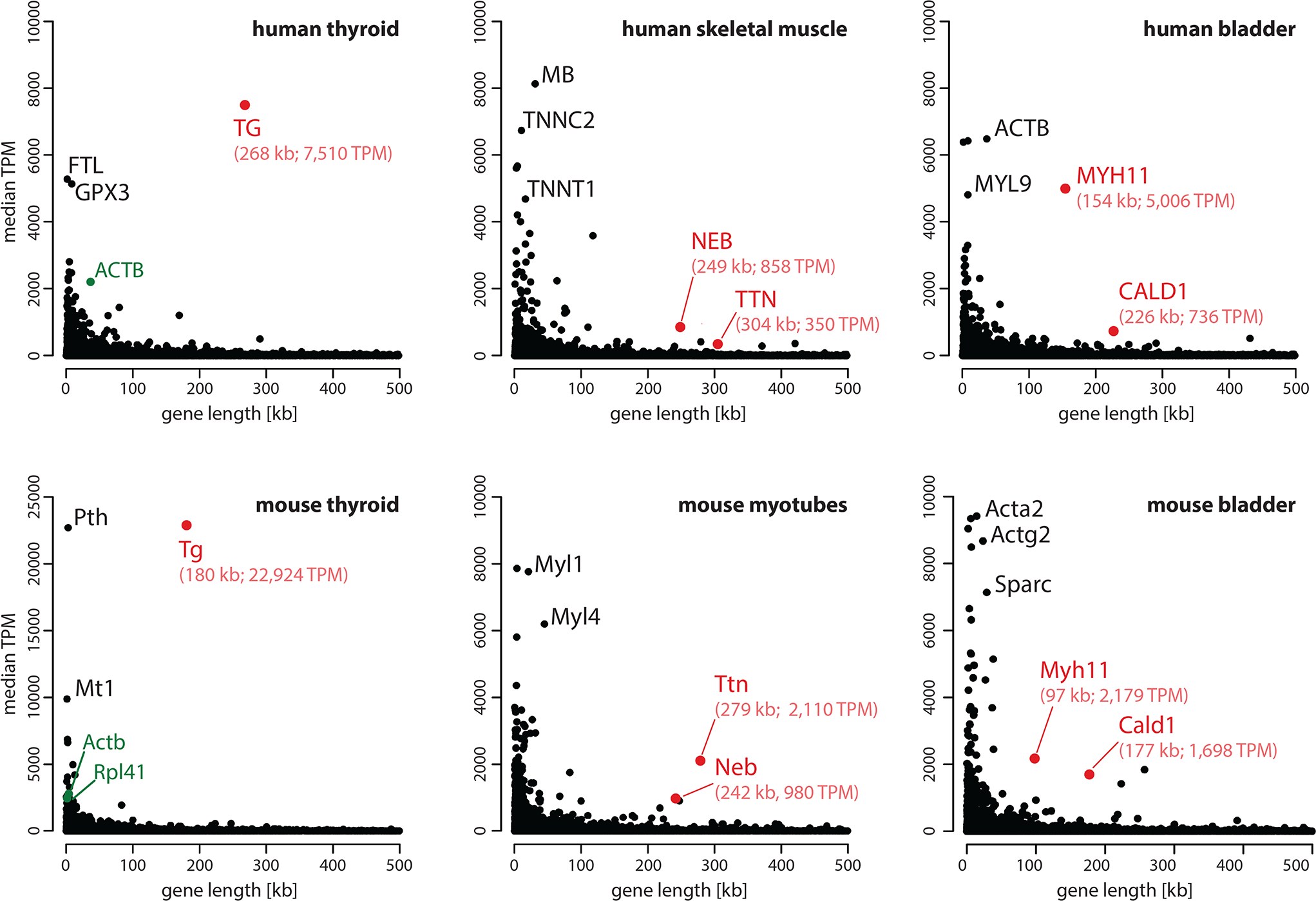
a, Analysis of gene expression in selected human tissues (retrieved from the GTEx database). b, RNA-seq analysis of corresponding mouse tissues and cells from this study. Expression level (median TPM) is plotted against gene length according to GENCODE. Candidate genes with a length of ca. 100 kb or longer and an expression level of ca. 1,000 TPM or above are marked in red. Note the exceptionally high level of Tg expression, exceeding the expression of housekeeping genes, such as Actb and Rpl41 (marked in green). Tg, thyroglobulin; Ttn, titin; Neb, nebulin; Myh11, myosin heavy chain 11; Cald1, caldesmon 1; Actb, beta-actin; Rpl41, large ribosomal subunit protein EL41. For data on all protein coding genes see Supplementary Tables 1 (human) and 2 (mouse).

Next, we performed RNA-seq analysis of mouse thyroid gland, myotubes, myoblasts and bladder to confirm the high expression of these five genes in the corresponding mouse cells (Supplementary Table 2). In particular, the mouse thyroglobulin gene (Tg, 180 kb) is exceptionally upregulated (22,924 TPM, constituting 2.5% of all sequence reads) with an expression level 10 times higher than that of some ubiquitously expressed housekeeping genes, such as non-muscle actin (Actb; 2,791 TPM) or ribosomal protein Rpl41 (2,467 TPM). All five selected mouse genes – Tg, Ttn, Neb, Cald1, Myh11 – met the conditions we have defined as prerequisites for our study (Fig.1b).

Highly expressed long genes form Transcription Loops.

Using genomic BAC probes encompassing the selected genes (Supplementary Table 3), we carried out DNA-FISH on cryosections of the corresponding mouse tissues – thyroid gland (Tg), skeletal muscle (Ttn and Neb), heart muscle (Ttn), bladder and colon (Myh11 and Cald1), as well as on cultured myoblasts (Cald1) and myotubes (Ttn and Neb). DNA-FISH, which includes RNase treatment and denaturation of cellular DNA, yielded two different signal patterns that were dependent on the expression status of the genes. In the non-expressed state, genes were condensed into single compact foci sequestered to the nuclear periphery (Fig.2a). In the expressed state, genes were strongly decondensed and exhibited several smaller foci in the nuclear interior (Fig.2b; Supplementary Figure 1).

Figure 2. Highly expressed long genes form Transcription Loops (TLs).

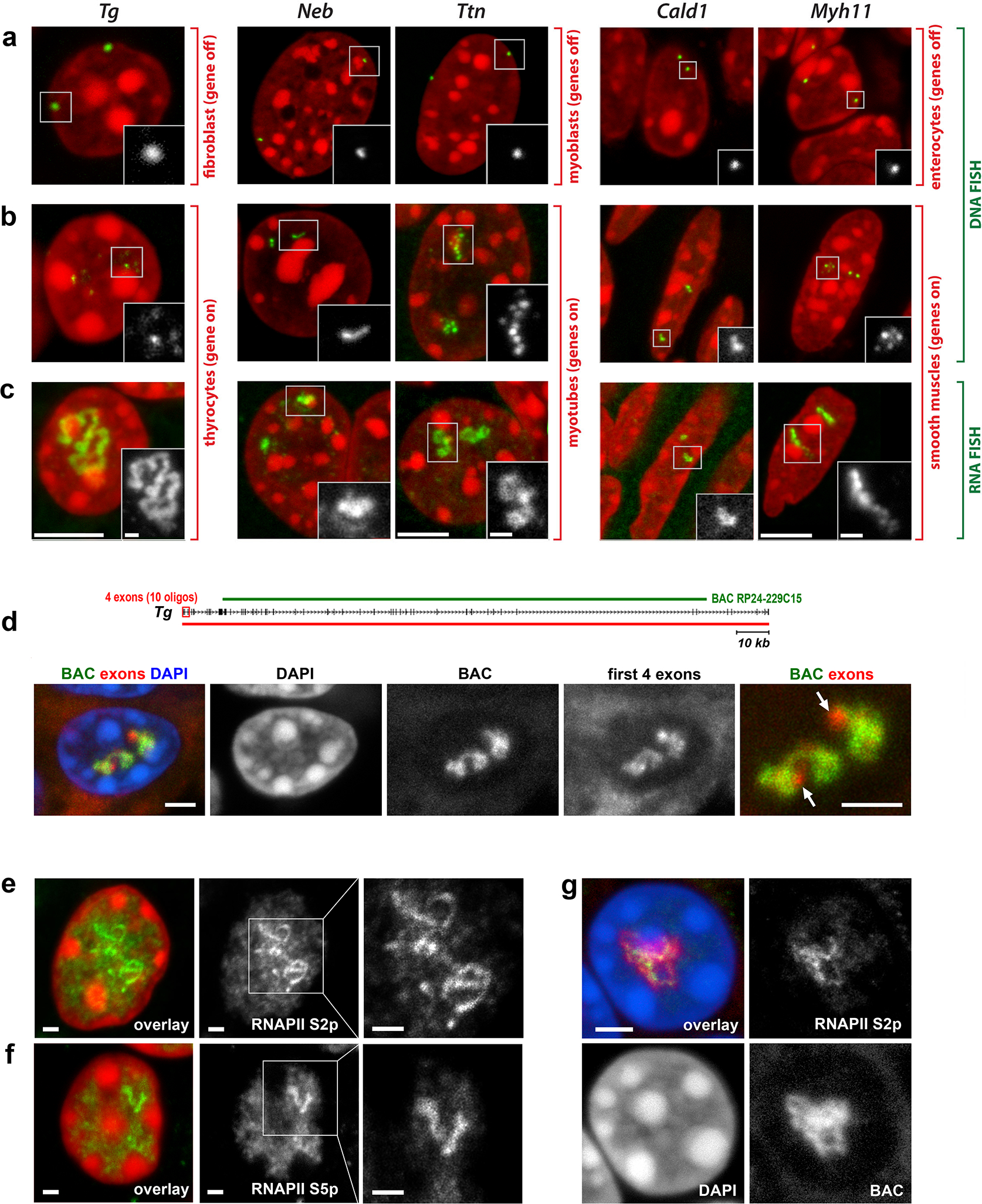
a-c, Five selected genes after either DNA-FISH (a,b) or RNA-FISH (c) with corresponding genomic probes. Control cells not expressing the respective genes exhibit focus-like condensed DNA signals at the nuclear periphery (a); in expressing cells, genes are strongly decondensed (b). RNA-FISH reveals TLs by hybridization to multiple nRNAs decorating the genes (c). d, The entire Tg TL detected by an oligoprobe, hybridizing to the first 5’ exons. The schematic shows distribution of the BAC covering the mid-part of Tg (green line) and the oligoprobe for the first 4 exons (red rectangle). Arrows point at Tg TL regions labeled by the oligoprobe but not by the BAC probe. e,f, Tg TLs revealed by immunostaining of the elongating (e, Ser2p) and initiating (f, Ser5p) forms of RNAPII. g, Immuno-FISH showing colocalization of structures marked with elongating RNAPII and Tg TLs. Images are projections of 1–2.5 μm confocal stacks. Scale bars: a-c, 5 μm, in insertions, 1 μm; d, g, 2 μm; e,f, 1 μm. Data represent 10 (a-c) and 2 (d-g) independent experiments.

Next, we performed RNA-FISH on the same set of samples, omitting both RNase treatment and cellular DNA denaturation. With this setup, the same genomic probes used for DNA-FISH hybridize to nRNAs. As expected, cells not expressing the genes were lacking FISH signals, whereas expressing cells exhibited massive RNA signals (Fig.2c, Extended Data Fig.2; Supplementary Figure 1). The signals were extended and either had the shape of a coiled loop (e.g., Tg, Ttn), or formed less discernible elongated structures (e.g., Neb, Cald1). The loops were particularly prominent in the case of the Tg gene – they were spread throughout the nuclear interior and measured up to 10 μm (Extended Data Fig.2a; Supplementary Figure 1; Supplementary video 1).

Since introns, as a rule, are substantially longer than exons, we assumed that the used genomic probes hybridized mostly to unspliced introns of nRNAs, thereby outlining the contours of transcribed genes. An expressed gene can also be visualized in its entirety by using oligoprobes hybridizing to the first 5’ exons (Fig.2d). In agreement with FISH data, immunostaining of initiating RNAPII (Ser5p) in thyrocytes highlighted short stretches of Tg gene, whereas immunostaining of elongating RNAPII (Ser2p) revealed strongly convoluted structures (Fig.2e,f) colocalizing with RNA-FISH signals (Fig.2g) and apparently corresponding to the Tg gene axis covered by polymerases. Hereafter we refer to these structures as Transcription Loops (TLs).

TL signals varied in shape and degree of coiling, and no consistent pattern of loop folding or position was observed with exception to their invariably interior nuclear location. Importantly, almost every single fully differentiated thyrocyte, skeletal muscle, heart muscle, or smooth muscle cell exhibited two TLs corresponding to two alleles. Scoring of RNA-FISH signals revealed that only a very small proportion of nuclei had one TL, as a result of either a long transcription pause, or monoallelic expression (Supplementary Table 4; Supplementary Figure 2).

At the level of light microscopy one can trace only the general contour of the TLs, but within this contour there is a finer coiling of the gene axis not resolvable by deconvolution or high-resolution microscopy (Extended Data Fig.3a). To demonstrate the inner structure of TLs, we performed FISH with the Tg probe on thin thyroid sections (50–70 nm) and indeed observed such coiling (Extended Data Fig.3b). Therefore, the compaction level of Tg TLs compatible with nucleosomal chromatin (ca. 17 kb/μm), which was calculated based on contour length measurements (Extended Data Fig.3c), is rather an overestimation. We cannot exclude that during Tg transcription a significant proportion of nucleosomes is lost, in agreement with the observations made for highly expressed ribosomal genes²¹ or lampbrush chromosome lateral loops²².

TLs manifest progression of transcription and splicing.

To confirm that the observed RNA signals are not accumulations of messenger RNAs (mRNAs) but represent nRNAs, we performed two types of RNA-FISH experiments. Firstly, we used differentially labeled probes hybridizing to 5’ exons (2–12) and 3’ exons (33–47) of the Tg gene. We reasoned that if loops represent mere mRNA accumulations, both probes would label the entire structures. The probe for 3’ exons, however, labeled only the second half of TLs (Fig.3a), confirming that TLs are decorated with growing nRNAs. On a smaller scale, we demonstrated that the oligoprobe for the 5’ half of Tg long intron 41 labels the entire intron, whereas the oligoprobe for the 3’ half of the intron labels only half of it (Fig.3b).

Figure 3. TLs manifest transcription progression and dynamically modify the harboring chromosomal loci.

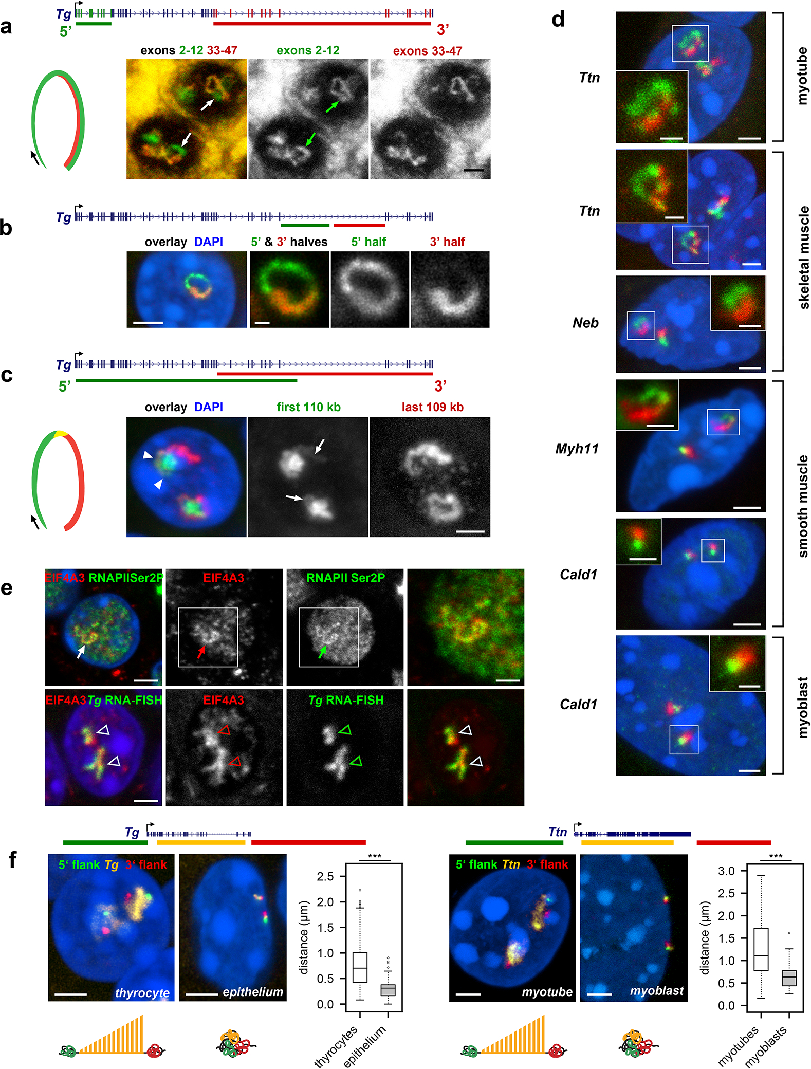
a, Successive labeling of Tg TLs with probes for 5’ (green) and 3’ (red) exons reflecting changes in exon composition. Arrows point at the TL regions labeled with only the 5’ probe. b, Successive labeling of the Tg long intron 41 with oligoprobes for the entire intron (green) and for its second 3’ half (red). c, Sequential labeling of Tg TLs with genomic probes highlighting 5’ (green) and 3’ (red) introns reflecting changes in the intron composition. The 5’ genomic probe includes 5’ exons and thus faintly labels the second half of the loop (arrows). Arrowheads mark the region hybridized by both overlapping probes. d, TLs formed by other long highly expressed genes exhibit co-transcriptional splicing. e, Colocalization of the component of the exon-junction complex EIF4A3 (red) with Tg TLs (green) visualized either by RNAPII staining or by RNA-FISH. In a-e, data represent 3 independent experiments. f, Expressed genes expand and separate their flanks. Distances between 5’ (green) and 3’ (red) flanking regions of the Tg and Ttn genes (yellow) are larger in cells expressing the genes compared to control cells with silent genes. Projections of confocal sections through 1 – 3 μm. Scale bars, 2 μm, in insertions on d and e, 1 μm. The distribution of the used probes in respect to the studied genes are depicted above the image panels. The boxplots depict the 3D distance between the flanking regions in expressing and non-expressing cells. The median inter-flank distance for Tg in thyrocytes is 2.3-fold larger than in control epithelial cells (703 nm versus 311 nm) (n = 203 alleles in thyrocytes and 180 alleles in epithelial cells across 2 independent experiments, ***p = 2.167×10⁻³⁴, two-sided Wilcoxon rank sum test). The median inter-flank distance for Ttn in myotubes is 1.7-fold larger than in control myoblasts (1,104 nm versus 634 nm) (n = 117 alleles in myotubes and 63 alleles in myoblasts across 3 independent experiments), ***p = 2.584×10⁻¹¹, two-sided Wilcoxon rank sum test). Boxplots show the median (horizontal line), 25th to 75th percentiles (boxes), and 90% (whiskers) of the group.

Secondly, we used genomic probes highlighting 5’ and 3’ introns. We expected that the two probes hybridize to nRNAs on TLs in a consecutive manner as a result of co-transcriptional splicing and, indeed, observed such a pattern. The 5’ genomic probe strongly labeled the first half of the loop by hybridizing to nRNAs containing yet unspliced 5’ introns and the 3’ probe labeled the second half of the loop by hybridizing to yet unspliced 3’ introns (Fig.3c,d). The oligoprobes covering 1–5 kb of two sequentially positioned introns of Tg, Ttn and Cald1 labeled TLs only partially, producing separate and non-overlapping signals (Extended Data Fig.4), further confirming the ongoing splicing²³. In agreement with multiple splicing events occurring along highly expressed genes, TLs are decorated by components of exon-junction complexes and either closely adjacent to, or partly colocalize with nuclear speckles (Fig.3e; Extended Data Fig.5).

Besides TLs, RNA-FISH with genomic probes revealed numerous granular signals scattered throughout the nucleoplasm, representing either mRNA, or accumulations of spliced-out but not yet degraded introns (for detailed description see Extended Data Fig.6).

TLs are open loops with separated flanks.

One of the popular views on the structure of transcribed genes is that the physical interaction between the TSS and TTS is crucial for a high level of gene expression. Such an interaction has been proposed to act as a “bridge” for RNAPIIs enabling them to immediately reinitiate transcription after termination, i.e. to transcribe “in circles”²⁴. To assess whether the beginnings and the ends of the selected genes are proximal, we visualized TLs and their genomic flanks for Tg, Ttn and Myh11 genes and found that the 5’ and 3’ gene flanks are visibly separated in 85%, 87% and 90% of the respective alleles. In particular, 3D distance measurements between flanks showed that they can be separated by up to 2.2 μm (Tg) and 2.9 μm (Ttn), and that the inter-flank median distances are ca. 2 times larger compared to those in control cells not expressing the genes (Fig.3f). Together these findings demonstrate that, contrary to the “transcription cycle” hypothesis, TLs of long highly expressed genes are open-ended loops with separated flanks.

TLs are larger for more highly transcribed genes.

Although the different hybridization efficiencies of the used probes and the various image acquisition conditions do not allow a legitimate quantitative comparison of DNA and RNA signal sizes between genes, the qualitative comparison of signals suggests that gene length alone is not a good predictor of TL size. The TL size is rather defined by expression level: e.g., RNA-FISH signals of the longer Ttn gene are less expanded compared to those of the shorter but 10 times more highly expressed Tg gene (Fig. 4a,b). Not surprisingly, we also noticed that the size of RNA-FISH signals inversely correlates with the condensation of genes detected by DNA-FISH: the gene body of Tg is strongly decondensed and marked with only few faintly labeled foci, whereas the Ttn gene is more condensed and displays a chain of several larger foci (Fig. 4a,b). The Neb gene, expressed at a more than 2 times lower level than Ttn, typically exhibits even more prominent gene body condensation (Fig. 4c). The body of Dmd, the longest mammalian gene (ca. 2.3 Mb) with very low expression, remains fairly condensed (Fig. 4d).

Figure 4. Transcription Loop size is not determined by gene length but by expression level.

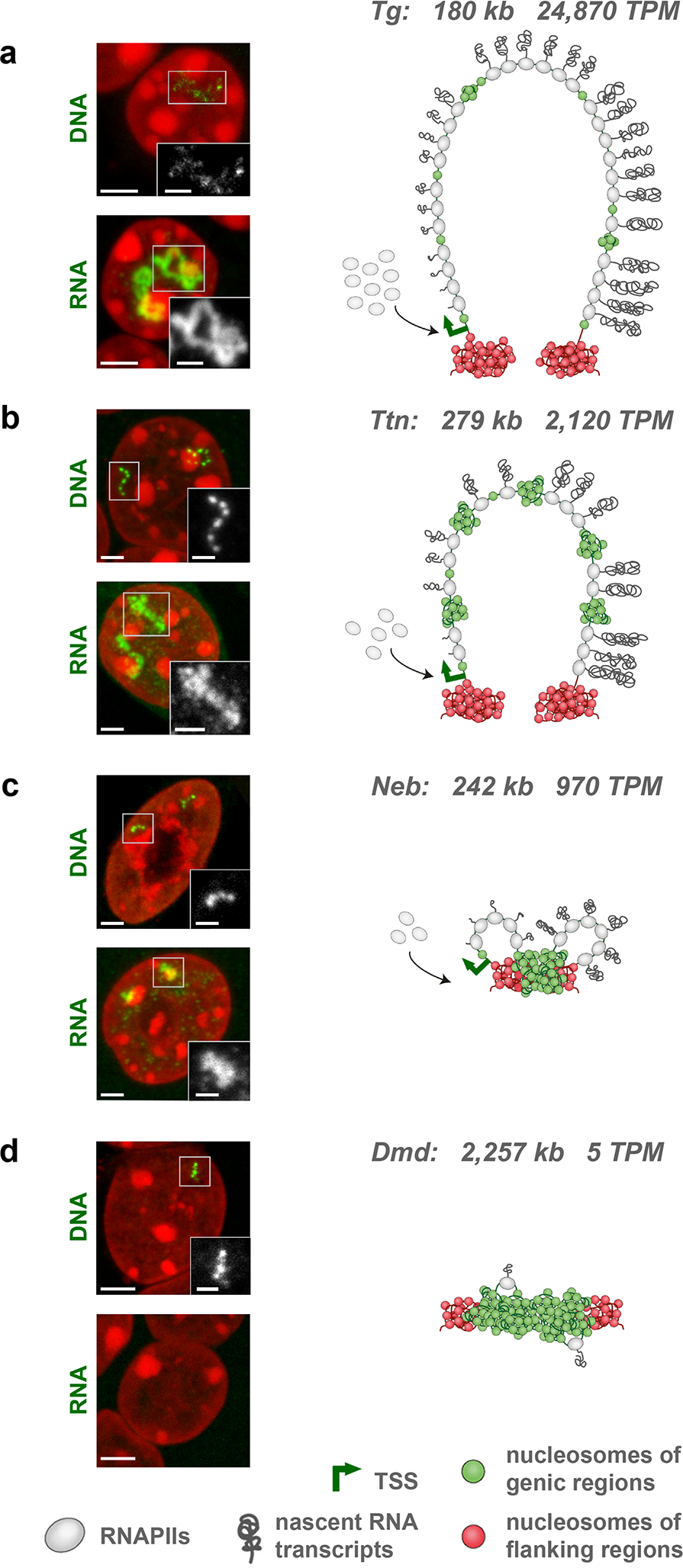
Examples of 4 long genes - Tg (a), Ttn (b), Neb (c) and Dmd (d) - arranged from top to bottom according to their expression level in the respective cell type. Gene length and expression level are indicated next to the gene symbol. For every gene two images are displayed on the left, showing DNA-FISH detecting the gene body and RNA-FISH detecting nRNAs. The more expressed a gene is, the less solid the DNA-signal is and the more expanded the RNA-signal is. Vice versa, the less expressed a gene is, the more condensed the gene body is and the less extended the RNA-signal is. The schematics on the right are speculative interpretations of the observed FISH signal patterns in terms of transcriptional bursts, depicted as RNAPII convoys with attached nRNAs, and transcriptional pauses, depicted as condensed chromatin (green nucleosomes). For simplicity, splicing events are not shown on the schemes. Microscopic images are projections of 1–1.5 μm confocal stacks. Scale bars, 2 μm, in insertions, 1 μm. Data represent 10 (a-c) and 4 (d) independent experiments.

The coordinated pattern of gene body condensation and TL expansion presumably reflects the frequency and duration of transcriptional bursts that are directly related to the expression level of genes²⁵. The possible scenario is that a highly expressed gene is transcribed in long and frequent bursts; an intermediately expressed gene – in short, less frequent bursts; the bursts of a lowly expressed gene are even shorter and less regular (Fig. 4). Consequently, in case of high expression, a gene is covered by long and frequent RNAPII convoys²⁶ and the entire gene body forms a transcription loop (e.g. Tg, Ttn). In case of lower expression, short and infrequent bursts do not decondense the entire gene but rather form short and sparse RNPII convoys leading to small “traveling” transcription loops (e.g., Neb, Cald1). In both cases, however, transcription occurs via the same mechanism with RNAPIIs moving along genes, which is evident from the sequential highlighting of introns.

TLs are dynamic structures.

To confirm that TLs are formed upon transcriptional activation, we performed several experiments to activate or inhibit Ttn transcription in vitro. First, we aimed to induce Ttn TLs in cells that do not express this gene and generated myoblasts stably expressing dCas9 conjugated with the tripartite transcription activator VP64-p65-Rta (VPR)²⁷. Targeting the dCas9-coupled activator to the Ttn promoter region induced expression of the full length gene in myoblasts (Supplementary Information Fig.3) to a level comparable to that in myotubes, which was accompanied by formation of Ttn TLs and by a 2-fold increase of Ttn median inter-flank distances (Fig.5a).

Figure 5. TLs are dynamic structures.

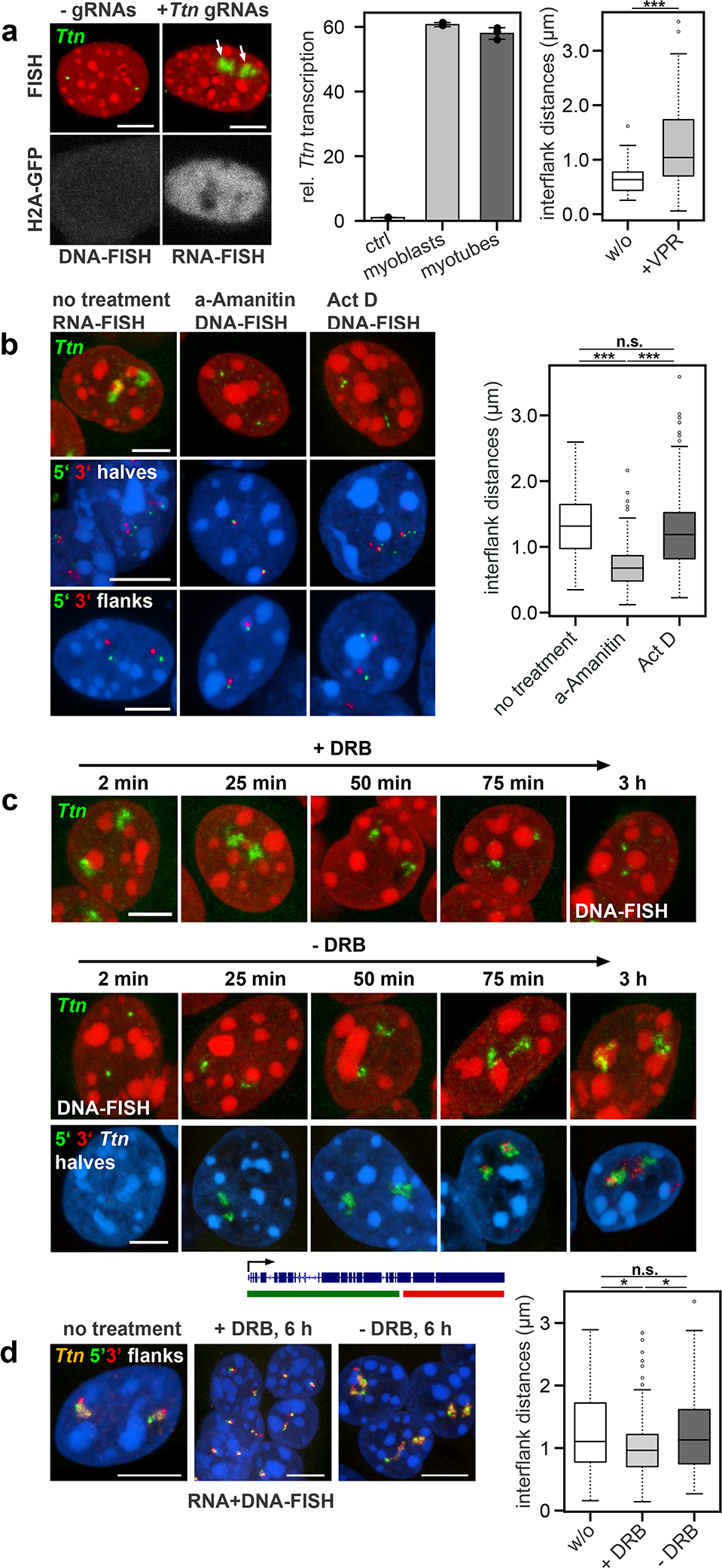
a, Ectopic induction of Ttn TLs in myoblasts by transfection of dCas9-VPR-expressing myoblasts with gRNAs targeting the Ttn promoter combined with H2A-GFP-plasmid. By this way, Ttn expression was induced to the level of myotubes (n=3, error bars depict standard deviations). 90% of transfected myoblasts exhibited Ttn TLs and a 2-fold increase in median inter-flank Ttn distances (1,039 vs. 634 nm) (n = 104 and 63 alleles collected from 52 and 70 cells across 2 independent experiments), ***p = 1.052×10⁻⁷, two sided Wilcoxon rank sum test). b, The transcription inhibitors α-amanitin and actinomycin D eliminate Ttn TLs in myotubes. α-amanitin-treatment causes strong condensation of the gene body and convergence of the flanks, whereas actinomycin D leaves the gene body decondensed and flanks diverged (n = 62, 79 and 112 alleles without treatment, alpha-amanitin-treatment and actinomycin D-treatment, collected from 140 myotube nuclei across 3 independent experiments), ***p = 5.5×10⁻¹², n.s. p = 0.110 for untreated cells versus alpha-amanitin-treatment and actinomycin D-treatment respectively, ***p = 4.669×10⁻¹⁰ for alpha-amanitin-treatment versus actinomycin D-treatment, two sided Wilcoxon rank sum test). c, DRB treatment leads to a gradual Ttn TLs shrinkage (upper panel); removal of DRB leads to a gradual TLs restoration (mid panel). Labeling of the 5’ (green) and 3’ (red) halves of Ttn allows to follow appearance of the 5’-end signal first following by the signal for 3’-end (bottom panel). d, Ttn inter-flank distances decrease after DRB-treatment (1,104 nm to 963 nm) but remain larger than inter-flank distances in myoblasts (634 nm); upon transcription restoration, the distances are restored (1,130 nm) (n = 117, 114 and 88 alleles collected from 160 myotube nuclei without treatment, after 6h of DRB-treatment and 6h after DRB-removal across 2 independent experiments), *p = 0.013, n.s. p = 0.899, *p = 0.026 for DRB-treated cells versus non treated cells, cells after DRB-removal versus non treated cells and DRB-treated cells versus cells after DRB-removal, two sided Wilcoxon rank sum test). Scale bars, 5 μm. a, b, d, Boxplots show the median (horizontal line), 25th to 75th percentiles (boxes), and 90% (whiskers) of the group.

Conversely, we aimed to eliminate Ttn TLs in differentiated myotubes by transcription inhibition. Incubation of myotubes with α-amanitin or actinomycin D led to abortion of RNAPIIs and disappearance of TLs (Fig.5b). In agreement with their different mechanisms of action²⁸, the drugs affected gene body condensation differently. In the case of α-amanitin, which prevents DNA and RNA translocation by binding near the catalytic site of RNAPII causing its stalling and degradation, the Ttn gene condensed and the gene flanks converged. In the case of actinomycin D, which prevents transcription initiation and RNAPII progression by intercalating into the DNA minor groove, Ttn remained decondensed with separated flanks (Fig.5b).

To further monitor TL dynamics, we treated differentiated myotubes with 5,6-Dichloro-1-β-D-ribofuranosylbenzimidazole (DRB), a drug reversibly preventing transcription elongation²⁸. As anticipated, during the first 2 hours of drug treatment, nRNA signals diminished and the gene body condensed. After drug removal, the TL signal gradually recovered with the 5’ signal emerging first and the 3’ signal emerging only after ca. 1 h (Fig.5c). In accordance with transcriptional changes, Ttn flanks converged upon drug application and diverged after drug removal (Fig.5d).

TLs can expand from harboring chromosomes.

Although the internal position of genes within their chromosome territory is compatible with transcription²⁹, very gene-dense and highly transcriptionally active chromosomal regions have been shown to significantly extend from chromosome territories for reasons that are not quite understood^30–34. To investigate the relationship between TLs and their harboring chromosomes, we visualized the Tg TL and chromosome 15 by FISH detecting both DNA and RNA. We found that Tg TLs are excluded from chromosomes and either expand into the nucleoplasm or coil next to the chromosome territory, forming their own “transcription territories” (Fig.6a). The areas of TLs are often depleted of chromatin, indicating an extremely high concentration of proteins involved in the massive transcription of Tg (Fig.6b). Remarkably, in 2% of Tg alleles, TLs split chromosome 15 territories into two halves with a gap marked by the 5’ and 3’ Tg flanking sequences and filled with Tg TLs (Fig.6c,d).

Figure 6. TLs are excluded from harboring chromosomes.

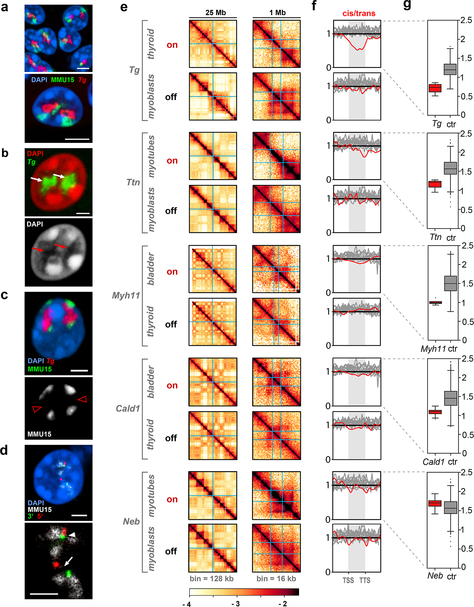
a, Tg TLs (red) emanate from the harboring chromosome 15 (green) and protrude into the nuclear interior. b, Nucleoplasmic regions occupied by Tg TLs (white arrows) are depleted of DAPI-stained chromatin (red arrows). c, Chromosomes 15 (green) are split into two halves by Tg TLs (red) with unpainted gaps (arrowheads). d, The gap in the chromosome territory (arrow) is marked with the 5’ (red) and 3’ (green) flanking sequences. The other chromosome territory is not split (arrowhead). Projections of confocal stacks through 1 μm; scale bars, a, 5 μm; b-d, 2 μm. In a-d, data represent 4 independent experiments. e, 25 Mb Hi-C contact map and a 1 Mb zoom view of five genes in active (on), or silent (off) states. TSS and TTS of the genes are marked with light blue lines (for detailed maps see Extended Data Fig. 7). f, Cis-to-trans ratio profiles, i.e. the total number of Hi-C contacts of a locus with loci on the same chromosome divided by the total number of contacts with other chromosomes, calculated for the gene of interest (red) and compared to 10 other long but lowly expressed genes (gray, see Supplementary Table 2 for the lists of genes). For comparison of cis-to-trans ratio profiles, the x-coordinates are rescaled so that the TSSs and TTSs of all genes are aligned (shaded areas). To highlight potential dips localized in the gene body against longer range variations, cis-to-trans ratio profiles are normalized to unity in the region outside the gene body. g, Statistical analysis of cis-to-trans ratios at a bin size of 32 kb for 5 studied genes (red) versus long but weakly expressed genes (gray). Tg, Ttn, Myh11 and Cald1 have significantly lower cis-to-trans ratios in comparison to control genes (0,735 vs. 1,196; 1,213 vs. 1,563; 0,987 vs. 1,498; 1,102 vs. 1,453, respectively) (p < 0.01, pairwise Mann-Whitney rank test for smaller values in the target group). Boxplots show the median (horizontal line), 25th to 75th percentiles (boxes), and interquartile range extended by 1.5 (whiskers) of the group. Hi-C assay was performed 3 times.

To further study the arrangement of TLs within their harboring chromosomes we performed Hi-C analysis of mouse thyroid, bladder, cultured myoblasts and myoblast-derived differentiated myotubes (Fig.6e; Extended Data Fig.7; Supplementary Information Fig.4). We reasoned that if an expressed gene loops out of the harboring chromosome, its cis-contacts are diminished compared to the cis-contacts of the same gene in a silent state, i.e. the cis-to-trans contact frequency ratio is expected to be low indicating externalization of the region. Analysis of Hi-C data revealed that cis-to-trans tracks of genes exhibiting the largest TLs (Tg, Ttn, Myh11 and Cald1, but not Neb that has lower expression) have dips, i.e. the genes are externalized, in contrast to the same genes in the silent state or other long but weakly expressed genes (Fig.6f,g). Notably, upon activation, Tg, Ttn, Neb and Myh11 relocate from B to A compartment (Extended Data Fig.8a), while Cald1 remains in A. While A-compartment regions are known to be externalized from their harboring chromosomes^35–37 (Extended Data Fig.8b), most TL-forming genes stand out in their degree of externalization compared to other genes on the same chromosome and with the same compartment signal (Extended Data Fig. 8d).

We asked whether similar mechanisms can lead to externalization of other active genes. While lower cis-to-trans ratio is associated with higher transcription and increasing gene lengths, these trends are due to a few (~100) very highly transcribed or very long genes (Extended Data Fig.8d,e). Among highly-transcribed (TPM>1000), longer genes are more externalized (R2=0.2–0.5; Fig 8e). Conversely, for long genes (>50 kb), the externalization increases with transcription (R2=0.12–0.28 for TPM=10²−10⁴). For all other genes the correlation of externalization with transcription and length is minute (R2<10⁻³). Thus, the externalization of genes from their harboring chromosomes is specific for long and highly expressed genes.

Figure 8. Polymer modeling of transcribed genes.

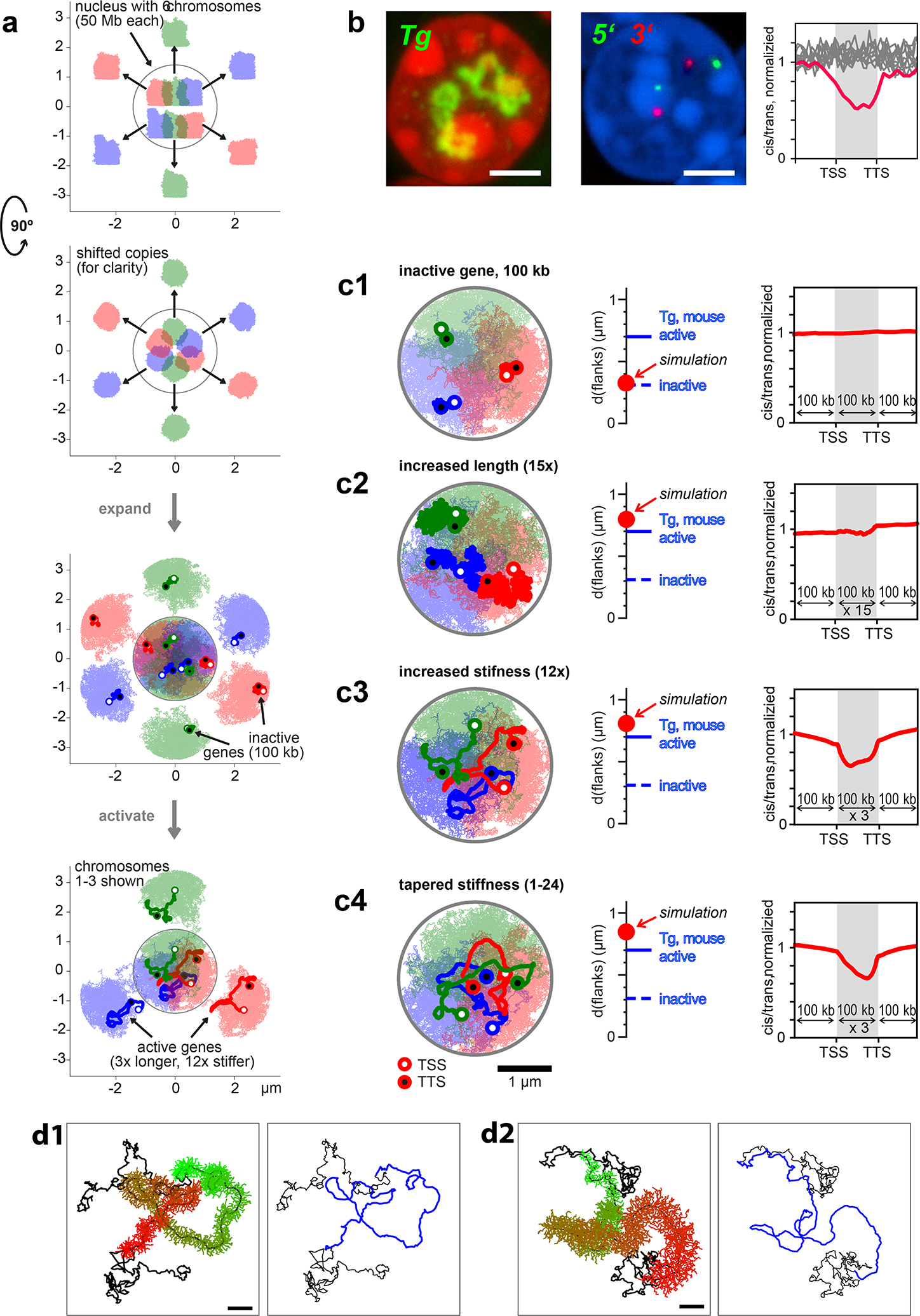
a, Polymer simulation setup. Six territorial chromosomes (50 Mb each) in a spherical nucleus were obtained by initiating them in a mitotic-like state (top and side view). For clarity, shifted copies are shown outside the nucleus. Then polymers were expanded and for each polymer, a 100 kb gene of interest was assigned (depicted with a darker color). In the rest of the simulations only 3 chromosomes are shown (bottom). b, Biological variables used to verify TL models: appearance of Tg TLs, inter-flank distances measured by microscopy and cis-to-trans contact ratios calculated from Hi-C maps; scale bar, 2 μm. c1, Genes of 100 kb are compact structures and do not exhibit a dip in cis-to-trans contact ratio compared to the surrounding fiber in the inactive state. c2, A mere increase in gene contour length (15-fold) leads to a bigger TL volume but doesn’t exhibit a clearly discernible contour or a dip in cis-to-trans contact ratio. c3, Increased stiffness (12-fold in the bending energy) together with a moderate increase in contour length (3-fold) shows that TLs expand substantially, exhibit a clear contour, and a dip in the cis-to-trans contact ratio. c4, A gradual increase in stiffness along the gene (on average 12-fold) leads to a larger flank separation, more coiling of the 5’ compared to 3’ gene ends and an asymmetric dip in cis-to-trans contact ratio with a steeper slope at the 3’ end. Scale bar, 1 μm. d, Side-chains as the source of increased stiffness: d1, a gene with 300 monomers, each decorated with 3 side-chains made of 5 monomers (colored from green to red), is shown together with the 300 monomer flanks (black). d2, sidechain length increases gradually from 1 to 15 monomers. Right panels show the backbone of the simulated genes (blue) from the left panels. Scale bars, 0.2 μm.

In contrast to the large-scale reorganization of TLs seen in microscopy, their effects in Hi-C are local as they do not alter long-range contacts across chromosomes (Extended Data Fig.9). We noticed two effects of TLs in Hi-C: (i) they perturb local cohesin-mediated organization (Tg, Ttn, Neb, Myh11) largely by diminishing or reorganizing TAD borders (Ttn, Neb, Myh11) and “dots” (Tg, Myh11) and (ii) several TLs show enrichment of self-interactions visible as “necks” (Ttn, Neb) or micro-domains (Myh11) (Extended Data Fig.7), similar to the observations in³⁸. Both phenomena could be related to the interplay of transcription and loop extrusion^{39, 40}. We concluded that TLs perturb the organization of their neighborhoods, leaving most of the harboring chromosomes unaffected.

TLs are stiff structures.

What makes highly expressed genes expand from chromosomes and separate their flanks? Every RNAPII complex is associated with a nascent ribonucleoprotein complex (nRNP) formed by newly synthesized nRNA and numerous proteins involved in RNA processing, quality control, transport, and translation⁴¹ (Fig.7a1). Therefore, nRNPs containing long nRNAs are bulky structures⁸ exceeding the size of nucleosomes (10 nm)⁴² or RNAPIIs (14 nm)⁴³. Since, during a transcription burst, RNAPIIs travel along a DNA-template as a tightly spaced convoy²⁶, we hypothesized that the dense decoration with bulky nRNPs turns a highly expressed gene into a stiff bottlebrush structure (Fig.7a2; Supplementary Video 2).

Figure 7. TLs of long highly expressed genes are stiff structures.

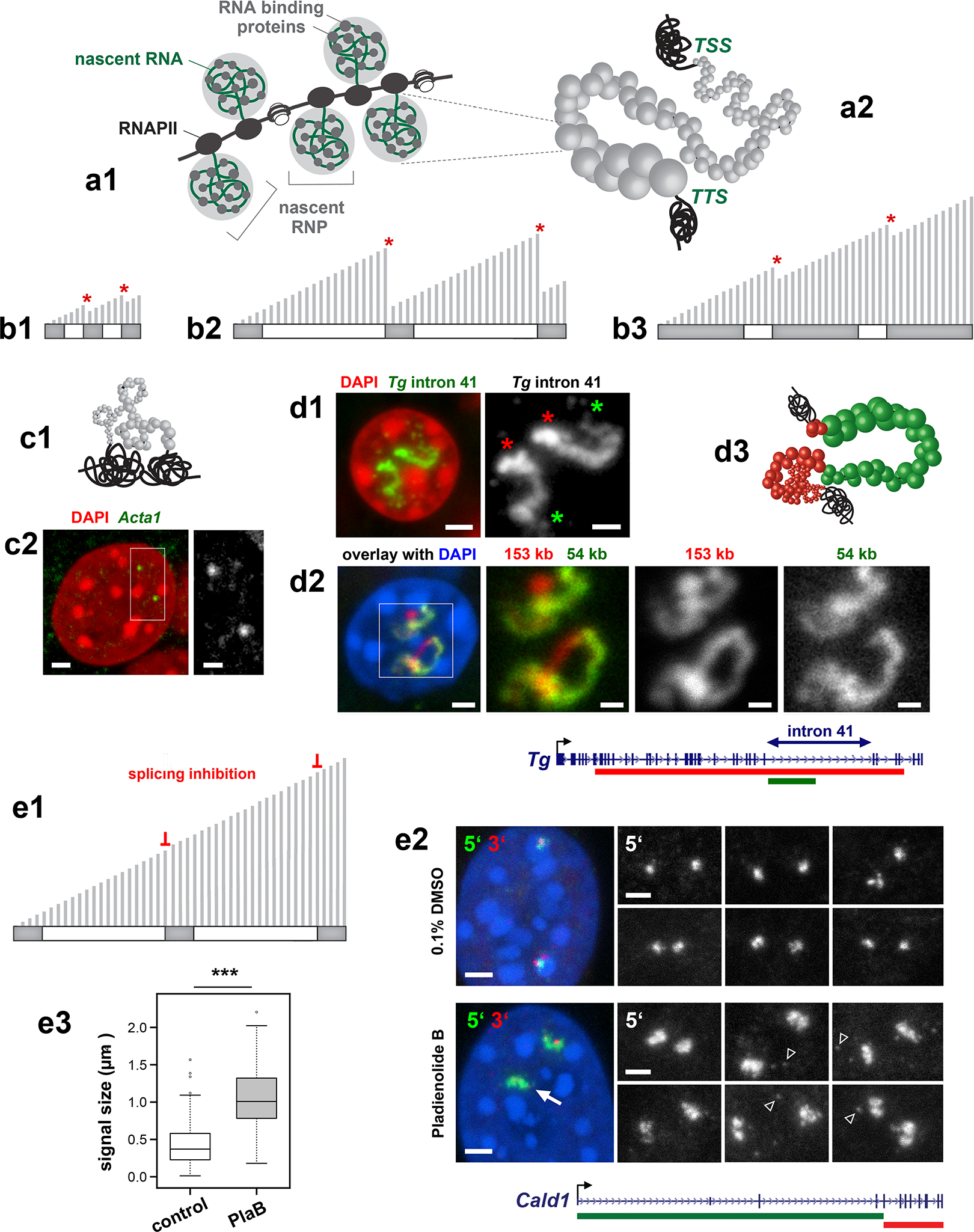
a, Cartoon depicting the nRNPs formed during transcription elongation (a1). nRNPs formed on a long highly expressed gene are voluminous and densely decorate the gene axis leading to its stiffness and expansion (a2). b, Schematics showing a short gene (b1), a long gene with long introns (b2) and a long gene with long exons (b3). Exons and introns are shown as dark-grey and white rectangles, respectively; transcripts are depicted as perpendicular light-grey lines of only half of the template length; splicing events are marked with red asterisks. c, Cartoon showing a short gene decorated by small RNPs allowing the gene axis to remain flexible and coil (c1) and example of highly expressed (4,360 TPM) but short (3 kb) Acta1 gene exhibiting a small RNA-FISH signal (c2). d, The longest Tg gene intron 41 (54 kb) strongly expands and exhibits a gradient of nRNPs from 5’ (green asterisks) to 3’ (red asterisks) splice sites (d1). The expansion of the intron (green) is disproportional in comparison to the rest of the gene (green, d2) as depicted in the cartoon (d3). Data represent 2 independent experiments). e, Schematic showing the effect of splicing inhibition on the length of nRNAs (e1). Comparison of Cald1 TL size signal in control myoblasts (0.1% DMSO) and myoblasts treated with the splicing inhibitor pladienolide B (10nM). RNA-FISH signals of the 5’ and 3’ ends are shown in green and red, respectively (e2). Gray-scale images show examples of the 5’ TL end. Pladienolide B causes massive abortion of transcription evident from the absence of the 3’ signal in a large proportion of Cald1 alleles (arrow) and accumulation of nucleoplasmic granules detected by the 5’ probe (arrowheads). Despite transcription abortion, the size of RNA-FISH signals is increased 2.5-fold indicating larger expansion of the TLs (e3; n= 118 and 123 alleles in DMSO and pladienolide B treated cells collected from 150 myoblasts across 2 independent experiments), ***p = 2.788×10⁻²⁵, two sided Wilcoxon rank sum test). Boxplots show the median (horizontal line), 25th to 75th percentiles (boxes), and 90% (whiskers) of the group. Scale bars: 2 μm, in close ups, 1 μm.

To become stiff, a bottlebrush has to be densely decorated by long sidechains⁴⁴. Short genes produce short nRNAs (Fig.7b1) corresponding to minute nRNPs, and hence cannot generate sufficient stiffness to prevent gene coiling even when a gene is highly transcribed (Fig.7c). In contrast, long genes produce long nRNAs corresponding to large nRNPs inducing stiffness and gene expansion. Large nRNPs can be formed on genes with either multiple long exons (Fig.7b3), or long introns (Fig.7b2). The first case is exemplified by the Ttn gene generating a 102 kb-long mRNA: the cis-to-trans ratio curve for Ttn displays an asymmetrical drop towards the 3’ end (Fig.6f), indicating a stronger exclusion of the 3’ gene end from the harboring locus. The second case is exemplified by the Tg gene with a 54 kb-long intron, over which mRNAs grow from ca. 6 to 60 kb, forming a signal gradient (Fig.7d1). The intron displays a disproportionately larger extension in comparison to the rest of the gene (Fig.7d2,3), consistent with greater stiffness. The strand opposite to Tg intron 41 includes the Sla gene, which is not expressed in thyrocytes (Supplementary Information Fig.5) and thus does not contribute to intron extension.

Next, we used splicing inhibition to increase the length of nRNAs experimentally, reasoning that this would lead to an increased size of nRNPs (Fig.7e1), which in turn would increase stiffness and, consequently, TL expansion. We inhibited splicing with pladienolide B⁴⁵ in myoblasts and performed RNA-FISH with probes for the intron-rich 5’ end and the exon-rich 3’ end of the Cald1 gene (Fig.7e2). Despite the massive abortion of transcription during drug treatment, we indeed observed a 2.5-fold increase of the signal size corresponding to Cald1 TL parts formed by the intron-rich region of the gene (Fig.7e3).

Polymer modeling confirms stiffness of TLs.

We next turned to polymer modeling aiming to understand whether stiffening and lengthening of a highly transcribed gene can give rise to a TL. We simulated 6 territorial chromosomes confined to a spherical nucleus by initiating them from a mitotic-like conformation and letting them expand (Fig.8a; see Methods and Extended Data Fig.10). On each chromosome, we modeled a 100 kb-long region as the gene of interest (Fig.8a,c1) and explored at which simulation parameters we can recapitulate the biological observables for the Tg gene: the appearance of TLs, distances between flanks measured by microscopy, and a dip in cis-to-trans contact ratio seen in Hi-C (Fig.8b).

First, we found that increasing gene length (by 15-fold due to nucelosomal loss: a 1 kb monomer extends from 20 nm to 300 nm) can increase the inter-flank distance, but fails to produce visible TLs (genes appear as amorphous clouds) or the dip in cis-to-trans ratio (Fig.8c2). Next, we reasoned that due to the dense decoration with nRNPs, a highly transcribed gene has an increased stiffness. When we increased the contour length by 3-fold (partial nucleosome loss) and altered the stiffness (bending energy) of the polymer, we found that a 12-fold increase in the stiffness reproduced the experimentally observed features of Tg TLs: the appearance of TLs, flank separation, and a dip in the cis-to-trans ratio (Fig.8c3). Moreover, the model recapitulates the dynamics of TL flanks upon gene silencing (Extended Data Fig.10b). Furthermore, to account for the gradual increase of the nRNA length along the gene, we introduced a tapered stiffness profile (from 1 to 24-fold), which caused (i) visibly more curled 5’ end and stretched 3’ end (Fig.8c4), recapitulating the Tg TLs, and (ii) asymmetric cis-to-trans profile along the gene, in agreement with Hi-C for the Ttn gene (Fig.6f).

Consistent with experiments, the appearance of simulated TLs does not lead to insulation of long-range contacts and is not accompanied by major changes in Hi-C maps, except the cis-trans dip (Extended Data Fig. 9 and 10c). This suggests that chromosomes, simulated and real, are sufficiently flexible to accommodate the formation of TL without major reorganization.

Since the biological foundation of our stiffness hypothesis is the dense decoration of genes with nRNPs, we simulated a polymer grafted with side-chains instead of imposing stiffness ad hoc. As expected from the theory^44, the region with side-chains expands, its flanks separate, and the backbone becomes progressively stiffer when we increase the sidechain length (Fig. 8d). Computed cis-to-trans profiles, however, did not have a clear dip indicating the lack of externalization, likely because other factors underlying chromosomal territoriality were not taken in account by modeling.

Importantly, simulations show that a sufficiently dense polymer system (nuclear chromatin) is not confining and allows large-scale relocalization of a long polymer loop (transcribed gene) subject to a sufficiently low force due to stiffening. In conclusion, our simulations serve as a proof of principle that increased stiffness can explain TL formation.

DISCUSSION

Our study focuses on the structure and spatial arrangement of individual transcribed genes in differentiated postmitotic cells and demonstrates that the sole process of transcription can have a profound effect on the spatial organization of gene loci by forming extended TLs, although functional implications of TLs remain to be understood. To enable light microscopy observations, we used relatively long highly expressed genes as a model and demonstrated that the selected genes form open-ended TLs visually resembling lateral loops of lampbrush^{7, 22} and puffs of polytene chromosomes⁸. Importantly, TLs are formed as a result of transcription and as such should not be confused with enhancer-promoter interactions or loops extruded by SMC complexes⁴⁶.

The sequential patterns of exon and intron labeling along TLs strongly indicate that RNAPIIs move along the gene axis and carry nRNAs undergoing splicing (Supplementary Video 2). This mechanism is drastically different from the model of transcription factories with immobilized RNAPIIs and nRNAs extruded in a spot^{12, 13}. TLs however do not contradict the notion of transcription condensates^{2, 47–49} that form and dissolve at different transcription stages^{50, 51}, although present at much smaller scales (submicrons versus microns).

We show that transcription dynamically modifies the chromosomal locus harboring a TL: transcription activation causes divergence of flanks and gene externalization from chromosome territory, whereas transcription silencing causes gene body condensation and convergence of its flanks. Separation of TL flanks argues against the proclaimed necessity of TSS-TTS association for maintenance of a high transcription level^52–54. Moreover, the complicated geometry of highly extended TLs is not compatible with the idea of a perpetual contact between a promoter or an enhancer-promoter complex with the gene body during transcription^{55, 56}.

The spreading of TLs over euchromatic nuclear areas by extending away from harboring chromosomes and even breaking them apart challenges the significance of chromosome territoriality in transcription regulation⁵⁷. A greater number of Hi-C trans-contacts for both euchromatin in general and long highly expressed genes, in particular, indicates that expressed genes can extensively interact with the surrounding euchromatin. Taken together, these data argue that chromosome territoriality is not an essential functional feature of the interphase nucleus, as was recently demonstrated⁵¹, but likely a mere consequence of the last mitosis⁵. Furthermore, the observed repositioning of a gene by several microns, together with polymer simulations, suggest that the nuclear environment is not confining but allows large-scale chromosomal movements, in agreement with recent chromosome micromanipulation⁵⁸ and arguing against proposals that interphase chromatin is a gel⁵⁹ or a solid⁶⁰.

We present evidence that highly expressed genes can generate a mechanical force sufficient to expand and re-localize them in nuclear space. We rule out the loss of histones as a possible mechanism as it causes gene lengthening but not externalization and TL formation. We suggest that TLs are characterized by increased stiffness caused by a dense decoration of the gene with progressively growing nRNPs. The hypothesis is supported by differential extension of TL regions with different sizes of nRNAs and by modeling a transcribed gene as a region of increased stiffness. This hypothesis also explains why highly expressed but short genes do not form resolvable TLs: a short gene lacks long introns or exons and is thus decorated by small nRNPs permitting gene-axis coiling (Fig.7).

In conclusion, we argue that while formation of microscopically resolvable transcription loops can be specific for long and highly expressed genes (Fig.4), the mechanisms underlying the formation of such loops can be a general aspect of eukaryotic transcription (Supplementary Video 2).

METHODS

GTEx data analysis.

RNA-seq data on human tissues was downloaded from the website of the GTEx portal (https://gtexportal.org/home/datasets, version 7, median gene level TPMs). The Genotype-Tissue Expression (GTEx) Project was supported by the Common Fund of the Office of the Director of the National Institutes of Health, and by NCI, NHGRI, NHLBI, NIDA, NIMH, and NINDS. GENCODE gene annotation version v19 (human) was downloaded from https://www.gencodegenes.org/. Using R (https://www.R-project.org/), mitochondrial genes were excluded from the analysis and only protein-coding genes with a known gene status were selected. Gene lengths were calculated from GENCODE annotated start and end positions of each gene. GENCODE annotations were joined with GTEx RNA-seq data based on the genes’ Ensembl ID (Supplementary Table 1).

RNA-seq.

Total RNA from cells or tissues was isolated using the NucleoSpin RNA Kit (Macherey-Nagel) according to the manufacturer’s instructions. Digital gene expression libraries for RNA-seq were produced using a modified version of single-cell RNA barcoding sequencing (SCRB-seq) optimized to accommodate bulk cells^{61, 62}. After digestion, purification and reverse transcription, the segments were subjected to Illumina sequencing adapters. During the library preparation PCR, 3′ ends were enriched with a custom P5 primer (P5NEXTPT5, Integrated DNA Technologies). Paired-end sequencing of the Nextera XT RNA-seq library was performed using a high output flow cell on an Illumina HiSeq 1500. In the first read, 16 bases were sequenced to obtain the sample-specific barcodes, while the 50 bases in the second read provided the sequence of the cDNA fragment. As multiple libraries were sequenced in parallel on the flow cell, an additional 8 base i7 barcode read was performed.

RNA-seq libraries were processed and mapped to the mouse genome (mm10) using the zUMIs pipeline⁶³. UMI count tables were filtered for low counts using HTSFilter⁶⁴. GENCODE gene annotation version vM11 (mouse) was downloaded from https://www.gencodegenes.org/. Mitochondrial genes were excluded and only protein-coding genes with a known gene status were selected to ensure proper annotation and used for further evaluation. Gene lengths were calculated from GENCODE annotated start and end positions of each gene (Supplementary Table 2).

Cell culture.

The mouse myoblast cell line Pmi28 was grown in Nutrient Mixture F-10 Ham supplemented with 20% fetal bovine serum (FBS) and 1% Penicillin/Streptomycin at 37°C and 5% CO₂. For differentiation, cells were seeded at a density of 8 × 10⁴ cells/cm² and incubated in a differentiation medium (high glucose DMEM supplemented with 1% Penicillin/Streptomycin and 2% horse serum) at 37°C and 5% CO₂. Differentiation medium was replaced every 2 days. A sufficient number of myotubes typically formed after 3–4 days.

Manipulation of transcription and splicing.

Transcription stimulation was performed using a system previously described²⁷. Pmi28 mouse myoblasts were transfected with PB-TRE-dCas9-VPR (Addgene, ID 63800) and PiggyBac transposase (System Biosciences, #PB200PA-1) expression plasmids at a ratio of 3:1 with Lipofectamine 3000 (Invitrogen) according to the manufacturer’s instructions. Clones that stably integrated dCas9-VPR were selected with a medium containing 50 μg/ml hygromycin B (Sigma-Aldrich). Single cells were sorted by fluorescence activated cell sorting (BD Biosciences Aria II Sorter) and cultured for one week in the presence of hygromycin B. dCas9-VPR expression was induced with 1 μg/ml doxycyclin for 50 h. Individual clones were tested for dCas9-expression by western blot using a Cas9 antibody (Clontech, dilution 1:1000). For gRNA transfection, 3×10⁵ cells were seeded in 6 wells on coverslips and transfected with 2.5 μg of a mix of 6 different gRNA plasmids per target gene (Supplementary Table 3) at equimolar amounts with Lipofectamine 3000 according to the manufacturer’s instructions. To monitor transfection efficiency, a plasmid expressing GFP-H2A additionally to the respective gRNA (U6-gRNA-GFP-H2A) was generated: CMV-GFP-H2A was inserted into the pEX-A-U6-gRNA expression plasmid via Gibson assembly. pEX-A-U6-gRNA was synthesized at Eurofins MWG Operon according to⁶⁵. Then U6-gRNA-GFP-H2A was added to the gRNA cocktail. dCas9-VPR expression was induced after 12 h by addition of 1 μg/ml doxycyclin. After 50 h of doxycycline treatment the expression of full-length Ttn mRNA was verified by reverse transcription-PCR on sequences located at the 5’ and 3’ ends of the full-length Ttn transcript with the primers indicated in Supplementary Table 3. Afterwards the relative expression level of Ttn was assessed by quantitative real-time PCR on a LightCycler 480 II (Roche) using LightCycler 480 SYBR Green (Roche) according to the manufacturer’s instructions with the following primers: Ttn fwd (5’-GCCGCGCTAGATTGATGATC-3’) and Ttn rev (5’-TCTCGGCTGTCACAAGAAGCT-3’); see also S Table 4. All generated plasmids are available upon request.

For transcription inhibition in myotubes, differentiation medium was supplemented with 10 μg/ml actinomycin D (Sigma-Aldrich) for 12 or 24 h, or 25 μg/ml α-amanitin (Sigma-Aldrich) for 24 h, or 100 μM 5,6-dichloro-1-β-D-ribofuranosylbenzimidazol (DRB) (Sigma-Aldrich) for 3 or 6 h. Fixation time points of cells under DRB treatment or after DRB removal included 2 min, 25 min, 50 min, 75 min and 3 h.

For splicing inhibition in myoblasts, the culture medium was supplemented with 10 nM of pladienolide B (Cayman Chemical) for 4 h before fixation.

Preparation of samples for ChIP-seq and Hi-C.

Pmi28 myoblasts were detached using 0.25% Trypsin/1 mM EDTA for 3 min and pelleted. For native ChIP-seq, the pellet (roughly corresponding to 15×10⁶ myoblasts) was directly snap-frozen in liquid nitrogen and kept at −80 °C. For Hi-C, cells were resuspended in medium to a final volume of 10 ml. 666 μl of 16% formaldehyde were added (resulting in a final concentration of 1% formaldehyde); the tube was briefly shaken and then rotated for exactly 10 min at 21 °C. To quench the reaction, 593 μl of 2.5 M glycine were added; the tube was briefly shaken and left rotating for 5 min. After quenching, tubes were centrifuged for 5 min at 2,000 g and the supernatant was discarded. Cells were resuspended in 1.5 ml PBS, transferred into 2 ml-tubes, centrifuged at 2,000 g for 5 min at RT and the supernatant was discarded. The pellets were snap-frozen in liquid nitrogen and stored at −80 °C.

Myotube samples were collected as follows in order to separate differentiated myotubes from undifferentiated myoblasts: first, myotubes were gently trypsinized using 0.025% Trypsin/0.1 mM EDTA; when myotubes detached, leaving the majority of myoblasts still attached to the bottom of the dish, the supernatant containing myotubes and a proportion of detached myoblasts was transferred to a fresh 150 mm cell culture dish to allow the remaining myoblasts to re-adhere to a dish bottom. Since myotubes do not re-adhere, they were collected with the supernatant. For native ChIP-seq, the pellet (corresponding to 10×10⁶ myotubes) was snap-frozen in liquid nitrogen and kept at −80 °C. For Hi-C, myotubes were fixed and frozen in the same way as myoblasts. We estimated that our myotube samples contained not less than 10–20% myoblasts.

Mouse thyroids for Hi-C were prepared as follows: thyroid glands from three mice were dissected within 5–10 min and stored in medium containing TSH (DMEM/F-12; 20% FCS; Penicillin/Streptomycin; 2 mM L-Glut; 40 μg/ml vitamin C; 1 U/ml TSH) in a cell culture incubator at 37 °C. Glands were then processed one by one. The two lobes of each gland were cleaned from attached neighboring tissues under a binocular and placed back in the incubator in the same medium while the other glands were being processed. Finally, all six lobes were joined in 2 ml of DMEM without FCS, minced with micro-scissors into small pieces (5–6 from each lobe) and transferred to a 2 ml-tube using low retention tips. The tube was centrifuged at 800 × g for 5 min at RT and the supernatant was discarded. Tissue was resuspended in 1.5 ml of DMEM without FCS. 100 μl of 16% formaldehyde were added (resulting in a final concentration of 1% formaldehyde); the tube was briefly shaken and then rotated for exactly 10 min at 21 °C. To quench the reaction, 89 μl of 2.5 M glycine were added; the tube was briefly shaken and left rotating for 5 min. The tube was moved to ice and kept there for 0.5 h. After quenching, tubes were centrifuged for 10 min at 2000 × g and the supernatant was discarded. The pellets were snap-frozen in liquid nitrogen and kept at −80 °C. The same procedure was repeated with three other mice so that each biological replicate consisted of two tubes each containing cells from 6 thyroid lobes. We estimated that mouse thyroid gland contains 400,000 – 1,000,000 cells (thus not less than 3,000,000 cells per biological replicate) and that thyrocytes constitute ca. 60% of thyroid cells.

For smooth muscles, one mouse bladder per sample was used. The tissue was minced and fixed as described for thyroid. We estimated that bladder samples contained 40–50% of smooth muscle cells.

Native ChIP-seq.

Native ChIP-seq was performed as previously described^{66, 67} with the following alterations: IPs were carried out with S1 mononucleosomes derived from Pmi28 myoblasts or myotubes. Experiments were performed in independent duplicates. Per one IP reaction (500 μl), mononucleosomes from 5×10^6 cells were incubated with 5 μg of antibody (anti-RNA polymerase II CTD repeat YSPTSPS, 8WG16, Abcam ab817, PRID AB_306327) in rotating tubes at 4°C overnight. Then the antibody was post-coupled to magnetic beads (Dynabeads Protein G, Invitrogen) at 4°C for 3 h and the eluted IP DNA was Phenol/Chloroform/Isoamylalcohol extracted using MaXtract high density tubes (Qiagen) and ethanol-precipitated according to a standard protocol. Illumina sequencing libraries were prepared using the NEBNext Ultra II DNA Library Prep Kit for Illumina (New England Biolabs) and the NEBNext Multiplex Oligos for Illumina (New England Biolabs) according to the manufacturer’s instructions. ChIP-seq libraries were sequenced on an Illumina HiSeq 1500 platform using 50 bp single end nucleotide sequencing.

Hi-C.

3 Hi-C biological replicates were prepared for each of the studied cell types. Sample sizes were estimated as follows: 15 ×10^6 of myoblasts, 10×10^6 of myotube nuclei, 3 ×10^6 of thyroid cells (thyroids of 6 mice); the number of cells in a bladder was not estimated. Hi-C was performed as described by⁶⁸. Myoblasts and myotubes were split into 3 or 2 subsamples, respectively, each containing 5×10^6 cells, which were treated as separate samples until the DNA purification step when they were merged into one biological replicate. Chromatin was digested with the restriction enzyme DpnII (New England Biolabs) at 37° C overnight. Chromatin sonication and size selection were performed with some modifications to allow retrieval of a higher DNA quantity. Hi-C libraries were sequenced using 50 bp paired-end sequencing on an Illumina HiSeq 4000. For the number of reads obtained in each Hi-C experiment see Supplementary Table 4.

Hi-C data processing.

Fastq files were mapped to the mm10 genome using the distiller pipeline (http://github.com/mirnylab/distiller-nf). Hi-C interaction data was stored in the cooler format⁶⁹ Cooler: scalable storage for Hi-C data and other genomically labeled arrays (https://github.com/mirnylab/cooler). We always applied iterative correction to our data in order to remove biases as much as possible⁷⁰. For the reproducibility of the replicates, see Supplementary Figure 4. Cis-to-trans contact frequencies were calculated for each bin as the number of cis (same chromosome) contacts divided by the number of trans (different chromosome) contacts of that bin. This is repeated for all bins along the genome, resulting in a genomic track of cis-to-trans contact frequency ratios.

For a comparison plot of the cis-to-trans ratios across a number of genes the x-axis for each gene was rescaled so that TSS and TTS align. Interpolation was used to obtain the same number of points in each gene. The cis-to-trans ratios were normalized to regions outside the genes (to be precise: the region from TSS-3’ gene length to TSS-0.5’ gene length and TTS+0.5’ gene length to TTS+3’ gene length is used to normalize cis-to-trans profile to unity). This is done to highlight local changes in the cis-to-trans ratio associated with genes while suppressing longer-range variations. For statistical validation, cis-to-trans ratios were compared for every 32 kb bin of target and control genes (see Supplementary Table 2 for the list of control genes). The statistical test was a pairwise Mann-Whitney rank test for smaller values in the target group with significance p<0.01.

Mice and tissue sampling.

CD-1 mice were purchased from Charles River Laboratories, housed in individual cages with free access to food and water on a 12–12 light dark cycle at the Biocenter, Ludwig-Maximilians-University of Munich (LMU) and treated according to the standard protocol approved by the Animal Ethics Committee of LMU and The Committee on Animal Health and Care of the local governmental body of the state of Upper Bavaria, Germany. Mice were sacrificed by cervical dislocation after IsoFlo (Isofluran, Abbott) narcosis.

Isolated tissues were washed with PBS and then fixed with 4% paraformaldehyde (Carl Roth) solution in PBS for 12–20 h. After fixation, mouse tissues were washed with PBS, cryoprotected in a series of sucrose, and embedded in Tissue-Tek O.C.T. compound freezing medium (Sakura). Blocks were stored at − 80°C before cutting into 16–20 μm sections using a cryostat (Leica CM3050S). Cryosections were collected on Superfrost Plus slides (Thermo Scientific) and stored at − 80°C before use.

For preparation of thin sections, thyroid glands were fixed in a mixture of 2% paraformaldehyde and 0.1% glutaraldehyde in 300 mOsm cacodylate buffer (75 mM cacodylate, 75 mM NaCl, 2 mM MgCl₂) for 30 min and then immediately embedded into Lowicryl. Thin sections (50–70 nm) were prepared using Reichert Ultracut.

FISH probes.

BAC-derived FISH probes.

BAC clones encompassing the desired genomic region (Supplementary Table 3) were selected using the UCSC genome browser (https://genome.ucsc.edu/) and purchased from BACPAC Resources (Oakland children’s hospital) as agar stabs (https://bacpacresources.org/). BACs were purified via standard alkaline lysis or the NucleoBond Xtra Midi Kit (Macherey-Nagel), followed by amplification with the GenomiPhi Kit (GE Healthcare) according to the manufacturer’s instructions. BAC probes were labeled either directly with fluorophores (using fluorophore-dUTPs), or with haptens (biotin-dUTP, digoxigenin-dUTP) by nick translation. Labeling of dUTPs was performed as described in⁷¹.

Chromosome paints.

Whole chromosome paints were a kind gift from Nigel Carter and Johannes Wienberg (Cambridge). Paints were amplified and labeled with Biotin or Digoxigenin via DOP-PCR with a partially degenerate oligonucleotide primer (6MW primer: 5’- CCG ACT CGA GNN NNN NAT GTG G −3’, Eurogentec)⁷¹.

Tg exon probes.

Probes that specifically label exons 2–12 and 33–47 of Tg were generated by standard polymerase chain reaction (PCR) using a cDNA clone (transOMIC technologies, BC111467) as a template. Primer sequences are listed in Supplementary Table 3. PCR amplified DNA was directly labeled with fluorophores by nick translation.

Oligoprobes.

Most of the oligoprobes were generated using the original SABER-FISH protocol⁷². BED files for the genomic locations of the exons and introns of the target genes were acquired from the UCSC Genome Browser. The designed oligos were ordered as oligo pools from IDT with a scale of 50 pmol/oligo. All used probe oligos are listed in Supplementary Table 3. The oligos were re-mapped if necessary for multi-color imaging and extended to ∼500 nt using the previously described primer exchange reaction⁷³. Finally, the probes were purified using PCR clean-up columns (Macherey Nagel).

Oligoprobes for Tg intron 41.

FISH probe generation was conducted as described previously for HD-FISH⁷⁴. The probe covering the first half of Tg intron 41 was amplified from genomic J1 ESC wt DNA. Primers to amplify fragments for FISH probes were designed with the HD-FISH probe generator platform accessible via http://www.hdfish.eu/⁷⁴ and are listed in Supplementary Table 3. After amplification, DNA was labeled with Alexa594 or Alexa647 using Ulysis Nucleic Acid Labeling Kits (Invitrogen).

FISH.

FISH on 3D-preserved cultured cells was performed as previously described^{71, 75, 76}. For DNA-FISH, cells were treated with 50 μg/ml RNase A at 37°C for 1 h. For DNA-FISH or FISH detecting both DNA and RNA, denaturation of both probe and sample DNA was carried out simultaneously on a hot block at 75°C for 3 min. For RNA-FISH, only the probe DNA, but not the sample DNA was denatured. Hybridizations were typically carried out in a water bath at 37°C for 2 days. Immuno-FISH was performed as previously described⁷⁵. Briefly, after immunostaining, cells were post-fixed with 2% PFA/PBS for 10 min, incubated in 20% glycerol for 1 h and further treated according to the protocol for 3D-FISH. RNA-FISH with oligoprobes (SABER-FISH) was performed by mounting SABER-probe containing hybridization mixture on fixed cells and incubating O/N at 43°C. The samples were washed with 2xSSC at 37°C 2x for 20 min and with 0.1xSSC at 60°C for 5 min. Hybridized SABER probes were detected by incubating with 1 μM fluorescently labeled detection oligonucleotides in PBS for 1 h at 37°C followed by washing with PBS for 10 min. FISH on cryosections was performed as previously described⁷⁷. Simultaneous denaturation of probes and sections was carried out on a hot block at 80°C for 3 min. For combined RNA-FISH and immunostaining, the cryosections were first hybridized with probes, then permeabilized with 0.1% Triton X-100/PBS and incubated with both primary and secondary antibodies as described previously^78–80.

The primary antibodies used in immuno-FISH experiments included rabbit anti-Cas9 (1:150 - Clontech, Cat# 632607), mouse anti-GFP (1:400 - Roche, Cat# 11814460001, PRID: AB_390913), mouse anti-RNAPII-Ser2ph (1:50 - clone 26B5, kind gift from Dr. H. Kimura, Tokyo Institute of Technology), rabbit anti-SON (1:50 - Sigma, Cat# HPA023535). Donkey anti-Mouse Alexa555 (1:250 - Invitrogen, Cat# A31570) and Donkey anti-Rabbit Alexa488 (1:250 - Invitrogen, Cat# A21202) were used as secondary antibodies.

In all experiments, nuclei were counterstained with 2 μg/ml DAPI in PBS for 10 min (cells) or 30 min (sections) and Vectashield (Vector) was used as an antifade mounting medium. For STED microscopy, nuclei were counterstained with SiR DNA and samples were mounted into Mowiol.

Microscopy.

Confocal image stacks were acquired using a TCS SP5 confocal microscope (Leica) using a Plan Apo 63/1.4 NA oil immersion objective and the Leica Application Suite Advanced Fluorescence (LAS AF) Software (Leica). Z step size was adjusted to an axial chromatic shift and typically was either 200 nm or 300 nm. XY pixel size varied from 20 to 60 nm. Axial chromatic shift correction, as well as building single grey-scale stacks, RGB-stacks, RGB-montages and RGB maximum intensity projections was performed using ImageJ plugin StackGroom⁸¹. The plugin is available upon request. For deconvolution of confocal stacks, a Lightning module of SP8 confocal microscope was used. High resolution microscopy of transcription loops after RNA-FISH was performed using either OMX (DeltaVision OMX V3 3D-SIM microscope, Applied Precision Imaging, GE Healthcare) equipped with lasers for DAPI and red fluorescence or with 3D STED (Abberior Instruments) with excitation pulsed lasers 594 and 640 nm and pulsed depletion laser at 775 nm.

Image analysis.

Inter-flank distances were measured using in-house semi-automated program. The signal spots in both channels were identified by detecting local minima in a Laplacian-of-Gaussian (LoG)-filtered image (with the expected size/sigmas set to enhance spots at the diffraction limit). A pairing of spots from both channels with minimal total distance was calculated using linear assignment and coordinates of both partners saved for further analysis. In both the detection and matching steps, results were visualized immediately, with the option to manually curate them and remove erroneous detection of pairings. The spot pair detection was implemented in Python in the form of a Jupyter notebook. The code is available at https://github.com/hoerldavid/fish_analysis.

The number of alleles in which inter-flank distances were measured: for thyrocytes, n=203 and for control epithelial cells, n=180; for myotubes, n=117 and for control myoblasts, n=63; for myotubes after irreversible transcription inhibition with alpha-amanitin, n=78 and actinomycin D, n=112 and for control untreated myotubes, n=62; for myotubes after reversible transcription inhibition with DRB for 6 h, n=113, after DRB removal, n=87 and for control untreated myotubes, n=116.

Contour length of the Tg TL regions were measured on maximum intensity projections of stacks after RNA-FISH. Loop contours were manually traced using the Segmented Line tool in ImageJ. For comparison of RNA-FISH signal size of Cald1 TLs in control cells and after splicing inhibition, maximum intensity projections of stacks after RNA-FISH were prepared and filtered (Gaussian = 1). The signal areas of individual Cald1 alleles were measured in Fiji after applying Intermodes threshold.

Transcription loop modeling.

Chromosomes were modeled as polymers with each monomer representing 1 kb or roughly 5 nucleosomes. To fix the three-dimensional (3D) size of a monomer, literature values for the compaction ratio c of the chromatin fiber, i.e. the number of bp per nm of contour length were used. Literature values vary greatly and are in the range c = 25 to 150 bp/nm^82–84. Here we used c = 50 bp/nm. We used a monomer size of 20 nm, corresponding to 5 nucleosomes or 1 kb.

For the Kuhn length l_K (typical bending radius of the fiber), again, literature values vary greatly and are in the range of l_K = 60 to 400 nm^82–84. Further estimations of the Kuhn length come from our own measurements of spatial distances of the 5’ and 3’ flanks of our genes in the inactive state (Fig.3). Those measurements suggest somewhat smaller Kuhn lengths between 25 and 80 nm. For our polymer model, we chose l_K = 56 nm or 2.8 kb.

Finally, we fixed the volume density of chromatin in the cell nucleus. It can be estimated from the genome size (≈ 3 Gb for a single copy, ≈ 6 Gb per nucleus) and the size of the nucleus. With a diameter of 8 μm we get a volume density of 180 bp in a cube of size (20 nm)³, or 0.18 monomers/(20 nm)³ which equals 18%. A cryo-EM measurement⁸⁵ suggests volume densities around 30%. For our polymer simulations we chose = 0.2 beads / (20 nm)^3 or = 20%.

In order to interpret simulations, the simulation time scale is converted to physical time. This conversion is done by comparing mean square displacements of simulation monomers with experimental data on tracked loci in yeast⁸⁶ and mammals⁸⁷ as described in⁸⁸. A conversion factor of 656 ps in simulations corresponding to 1s real time was obtained.

Polymer simulations were performed using a Mirny lab written wrapper (available at https://github.com/mirnylab/openmm-polymer-legacy) around the open source GPU-assisted molecular dynamics package Openmm ​(1,2). Polymers are represented as a chain of monomers with harmonic bonds, a repulsive excluded volume potential (3 k_BT), and are simulated with a collision rate of 0.1 inverse picoseconds (see⁸⁸ for details on simulation parameters and setup). We imposed an energetic cost of nonzero bond angles. Specifically, the potential energy for bond angles is E(α)=kα²k_BT/2. Unless otherwise mentioned (see below), we used k=1 to obtain the aforementioned Kuhn length.

We included A/B compartmentalization and lamina attraction. A/B compartmentalization was obtained by adding a weak attraction between monomers of type B (0.1 k_BT), which induces phase separation. The segmentation of our 50 Mb chromosomes into A and B compartmental segments is based on a random distribution. We used the same segmentation as in⁸⁸ but scaled up by a factor of 2.5 to account for the reduced coarse-graining. The mean compartmental segment size was 650 monomers or 650 kb. Furthermore, the association of B-type chromatin with the nuclear periphery was modeled by a weak attraction (0.6 k_BT) of B-type monomers with the sphere boundary representing the nuclear envelope. We point out that our simulation results on transcription loops do not depend on the presence of A/B compartments and lamina attraction.

Six chromosomes of 50 Mb each (corresponding to 50,000 monomers each) were simulated and placed inside a sphere with a diameter of 2.84 μm (corresponding to 42 monomer diameters). Territorial chromosomes were generated by initiating them in a mitotic-like conformation and letting them expand. In a dense environment, polymer dynamics is exceedingly slow, therefore, chromosomes mix only moderately and retain their territoriality over all simulated times, corresponding to at least hours, or days of real time. The above expansion from mitosis was repeated 10 times for 25 min and 24 s (1,000,000 simulation time units) each. These chromosome conformations served as initial conditions for our simulations of long highly transcribed genes. Simulations of transcription loops were then run for 127 min of real time (5,000,000 simulation time units), unless otherwise mentioned. We performed 30 runs (thus using each initial conformation three times). In each run, 101 conformations were saved at equidistant time points.

To simulate the effect of a high expression of a long gene, a 100 kb region (100 monomers) on each simulated chromosome was assigned to the gene of interest. First, in order to study the effect of a mere increase in contour length, we increased the region assigned as the gene of interest to cover a 15-fold longer region, i.e. 1,500 kb. The fiber properties - rigidity and monomer size - were not altered. Then, in order to study the effect of increased stiffness, in the 100 kb regions the bending rigidity of the fiber was increased. To simulate increased stiffness, the parameter k was increased from our default value of unity (see above) to the specified values, e.g. to 12. The 12-fold increase in the bending energy was chosen by sweeping a range of values and choosing one that best reproduces the experimentally measured end-to-end distance of TLs. The “genes” were positioned in a region of A-type chromatin.

Simulations of genes with side-chains were performed by attaching short side-chains onto monomers of the gene backbones. The side-chains were identical to the backbone in terms of monomer size, excluded volume potential and bond force. There was no bond angle energy within the sidechains. We attached 3 side-chains to each backbone monomer (other grafting densities yielded similar results). We used uniform sidechain length (5 monomers per side-chain, i.e. 100 nm side-chain length) as well as side-chain length gradually increasing from 1 to 15 monomers along the gene backbone.

To obtain Hi-C maps from simulated data, polymer conformations were coarse grained by a factor of 10 (i.e. only every 10th monomer is considered) in order to reduce the size of the computed Hi-C matrix. A cutoff radius was then designed mimicking the crosslinking radius in an actual Hi-C experiment. The cutoff radius was 10 monomer diameters. Hi-C maps were computed from conformations in the second half of each run. Cis-to-trans contact frequency ratio tracks were computed as for experimental Hi-C matrices. The cis-to-trans ratio tracks of all six simulated chromosomes were aggregated to improve statistics.

Statistics and reproducibility.

The experiments shown in this study were performed as 2–10 biologically independent experiments and no inconsistent results were observed. Data plotted as boxplots indicate the 25th and 75th percentiles, with the whiskers showing the minima and maxima (5th and 95th percentiles), black circles indicating the outliers and the horizontal line showing the median, if not stated otherwise. Some data are plotted in bar graphs as the mean ± s.d. If not stated otherwise, statistical testing was performed using the two-sided Wilcoxon rank-sum test. Details of the particular statistical analyses used, precise P values, statistical significance, number of independent biological replicates and sample sizes for all of the graphs are indicated in the figures or figure legends. No data were excluded. For the number of acquired nuclei after FISH experiments, see Supplementary Table 4.

DATA AVAILABILITY

Hi-C data have been uploaded to Gene Expression Omnibus (GEO) and are available under accession GSE150704. ChIP-seq and RNA-seq data are available at ArrayExpress (EMBL-EBI) under accession E-MTAB-9060 (https://www.ebi.ac.uk/arrayexpress/experiments/E-MTAB-9060/). Previously published reference genome mm10 and gene annotation of the C57BL/6J strain were downloaded from the Ensemble database (version: GRCm38, release 74). Source data are provided with this study. All other data supporting the findings of this study are available from the corresponding author on reasonable request.

CODE AVAILABILITY

The used code for the measurement of flank distances is available at https://github.com/hoerldavid/fish_analysis; code used for the analysis of Hi-C data (Cooler, Cooltools, Distiller, Pairtools is available at https://github.com/open2c; the code used for polymer simulations is available at https://github.com/mirnylab/openmm-polymer-legacy.

Extended Data

Extended Data Fig. 1. Long genes are rare and expressed at lower levels than short genes.

a, Analysis of gene length distribution within the human and mouse genomes showed that about 43% and 46% of all protein coding genes, respectively, have a length ≤20 kb and only 18% and 14% have a length of 100 kb or above. Bin size: 20 kb. Genes are annotated according to GENCODE. Only genes with a length <500 kb are shown. b, To select suitable genes for visualization with light microscopy, we studied gene expression profiles across 50 human tissues using the publicly available Genotype-Tissue Expression database (GTEx Consortium) and found that long genes, as a rule, are not highly expressed. For example, in liver (top) and brain (bottom) there were no expressed genes with both a length 100 kb and with a median expression ≥1,000 TPM. c, Comparison of RNAPII occupancy between short and long expressed genes. ChIP-seq with an antibody against the CTD of RNAPII in cultured mouse myoblasts (left) and in vitro differentiated myotubes (right). All genes, expressed (>1 TPM, blue) and silent (<1 TPM, red), were split into five categories according to their size. RNAPII density (Y-axis) is plotted against the respective position within the gene (X-axis); each gene is divided into 200 equally sized bins and genes from the same size category are aligned according to the bins. Expressed genes display a higher occupancy with RNAPII compared to non-expressed genes, especially in the TSS region. In the group of expressed genes, the RNAPII occupancy negatively correlates with gene length: the shorter the genes, the higher the RNAPII occupancy. d, Analysis of RNA-seq data for myoblasts (left) and myotubes (right). The median expression level is higher in groups containing shorter genes (<25 kb) and generally negatively correlates with gene length.

Extended Data Fig. 2. Visualization of the five selected genes in expressing and not expressing cells.

a, The Tg gene is expressed in thyrocytes where both alleles form prominent TLs expanding into the nuclear interior. In neighboring cells with a silent Tg gene - parathyroid gland cells, tracheal chondrocytes, epithelial cells, fibroblasts and muscles - Tg is highly condensed and sequestered to the nuclear periphery. b, The Ttn gene is expressed in skeletal muscle (b1), heart muscle (b2) and myotubes differentiated from Pmi28 myoblasts in vitro (b3). Note that only muscle nuclei (solid arrowheads) exhibit TLs. In muscle fibroblasts (arrows) or undifferentiated cultured myoblasts (empty arrowheads), Ttn is condensed at the nuclear periphery. c, The Neb gene is expressed in skeletal muscles and cultured myotubes, although to a lesser degree than Ttn. Accordingly, it forms smaller TLs. Arrowheads indicate muscle nuclei; arrows indicate fibroblast nuclei with silent Neb. d, e, The Myh11 (d) and Cald1 (e) genes are expressed in smooth muscles of colon and bladder where they form TLs. Note that after RNA-FISH, only smooth muscles (arrowheads) but not the neighboring epithelial cells (arrows) exhibit TLs. In addition, Cald1 is expressed in cultured myoblasts and forms small TLs in these cells. As indicated above the panels, images display signals after either RNA-FISH (no tissue/cell DNA denaturation and no RNasing), or simultaneous detection of DNA and RNA (tissue/cell DNA denaturation but no RNasing). All images are projections of 1–3 μm confocal stacks. Scale bars for overviews of skeletal muscle, colon and bladder, 50 μm; for the rest of the panels, 5 μm. Data represent 100 in a,b3 and 10 in b1,b2,c-e independent experiments.

Extended Data Fig. 3. Structure and compaction of TLs.

a, The internal structure of Tg and Ttn TLs is not resolvable after deconvolution (left) and high resolution microscopy (mid, right). b, Coiling and folding of TLs demonstrated in 50–70 nm thin resin sections. The upper panel shows thin sections through nuclei of thyrocytes stained with DAPI (red) and Tg TLs detected by RNA-FISH (green). The lower panel shows 2-fold close-ups of the corresponding Tg TL as grey-scale images. Note curling and twisting of the loops. Images are single optical sections. c, To assess the compaction level of TLs, the contour length of three Tg TL regions was measured on projections after RNA-FISH. The track of the Segmented Line tool in ImageJ, used for measurements, is shown on the right panel. Tg regions of 153 kb, 109 kb and 62 kb had a similar compaction level and measured 9 μm, 6 μm and 4 μm, respectively. These values correspond to a nucleosomal structure of chromatin (table on the right). However, since Tg TLs display internal structures and since the measurements were performed on maximum intensity projections, the compaction level of Tg TLs is probably overestimated. Scale bars: a, 2 μm; b,c, 1 μm. Data represent 3 independent experiments in a-c.

Extended Data Fig. 4. TLs manifest co-transcriptional splicing.

Two sequentially positioned introns were labeled with oligoprobes encompassing 1.2 – 5 kb. The schematics above the panels depict the distribution of oligoprobes (green and red rectangles), labeled introns (green and red lines) and positions of BAC probes used as references (grey lines above genes). After RNA-FISH the intron probes label TLs only partially and sequentially. Since the 5’ and 3’ intron signals do not overlap, the 5’ introns are spliced before the 3’ introns are read. For instance, in Cald1, introns 1 and 3 are separated by intron 2, suggesting that the “green” intron 1 is spliced out before polymerases reach the “red” intron 3, most likely after RNAPII runs over the 3’ splice-site of the first intron. Projections of confocal sections through 2 – 3.5 μm. Scale bars: 2 μm, in close-ups, 1 μm. Data represent 2 independent experiments.

Extended Data Fig. 5. Close association of TLs with splicing factors.

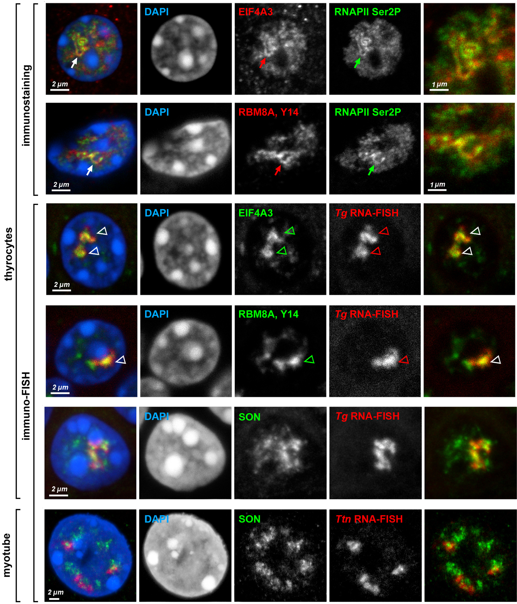
Splicing factors, SON and components of exon-junction complexes EIF4A3 and RBM8A (Y14), are either co-stained with RNAPII Ser2P (the two top rows) or visualized together with TLs in immuno-FISH (the rest of the rows). Note that signals of TLs and splicing factors colocalize only partly. The myotube nucleus is tetraploid and thus exhibits 4 Ttn RNA signals. Images are partial projections of either 0.6 μm (for immunostaining) or 0.9 μm (for immuno-FISH). Scale bars: 2 μm, in close-ups, 1 μm. Data represent 3 independent experiments.

Extended Data Fig. 6. Nucleoplasmic granules in cells with highly expressed long genes.

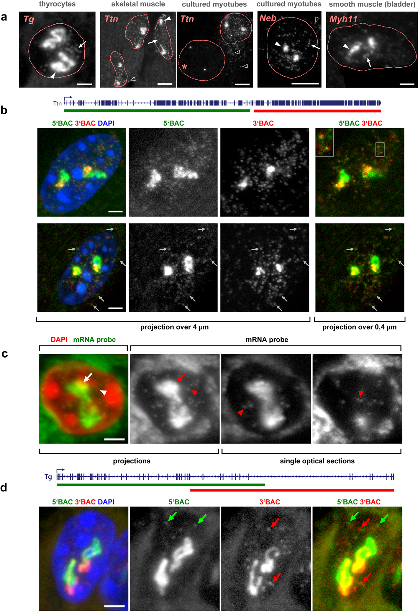
a, RNA-FISH reveals numerous nucleoplasmic granules (arrows) surrounding TLs (arrowheads) after hybridization with genomic probes. For clarity, only RNA signals are shown within the outlined nuclei. Empty arrowheads point at similar granules in the myotube cytoplasm. The asterisk marks the nucleus of a myoblast not expressing Ttn. b, In muscles and cultured myotubes, the majority of granules (81%) are double-labeled with probes for the 5’ and 3’ halves of Ttn and found in both the nucleoplasm and cytoplasm (arrows on the lower panel), thus likely representing Ttn mRNAs. Remarkably, the 5’ and 3’ signals are spatially distinguished within the granules (insertion) presumably due to the exceptionally long Ttn mRNA of ca 102 kb. The observed separation of the 5’ and 3’ halves of Ttn mRNA is in agreement with previously described structures of cytoplasmic mRNPs^28–30. c, In difference to Ttn, mRNAs of Tg, Neb, Cald1 and Myh11 genes are short (4 – 20 kb) and can be only detected with oligoprobes specifically hybridizing to all exons. Thus the oligoprobe for all 48 Tg exons hybridizes to nRNAs decorating TLs (arrows) and also labels multiple nucleoplasmic granules (arrowheads). d, The majority of the other thyrocyte nucleoplasmic granules are labeled with either 5 (green) or 3 (red) genomic probes with only 10% of granules being double-labeled. The brightness of the RNA-signal on the most right panel is purposely increased to highlight nucleoplasmic granules (green and red arrows). Such differential labeling of nucleoplasmic granules, exemplified here for thyrocytes, is characteristic for other studied genes and strongly suggests that these granules represent accumulations of excised introns. The distribution of the used BAC probes in respect to the studied genes are depicted above the image panels. Scale bars: a, 2 μm for Tg and Myh11, 5 μm for Ttn and Neb; b, c, d, 2 μm. Data represent 10 in a,b and 3 in c,d independent experiments.

Extended Data Fig. 7. Fragments of Hi-C maps around TL-forming genes in corresponding tissues and cells.

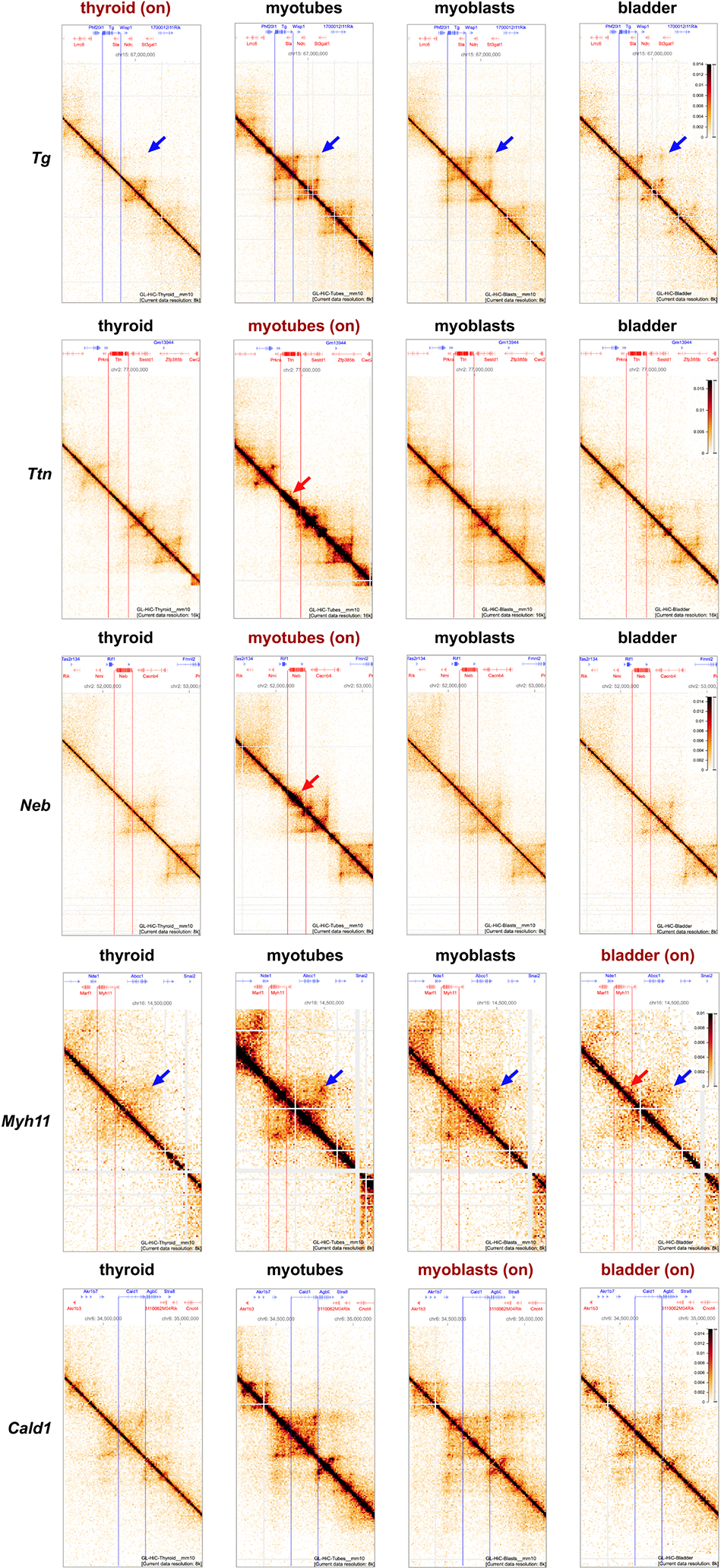
Each row shows the same region around indicated genes in different tissues or cells; “on” indicates a cell type where a gene is active, allowing to compare changes associated with TL formation. Blue arrows indicate loss of TAD borders and associated dots of CTCF-CTCF enrichment for expressed Tg and Myh11. Red arrows indicate an increase in self-interactions within genes visible for expressed Ttn, Neb and Myh11.

Extended Data Fig. 8. Cis-to-trans contact ratios and A/B compartments in studied cells.

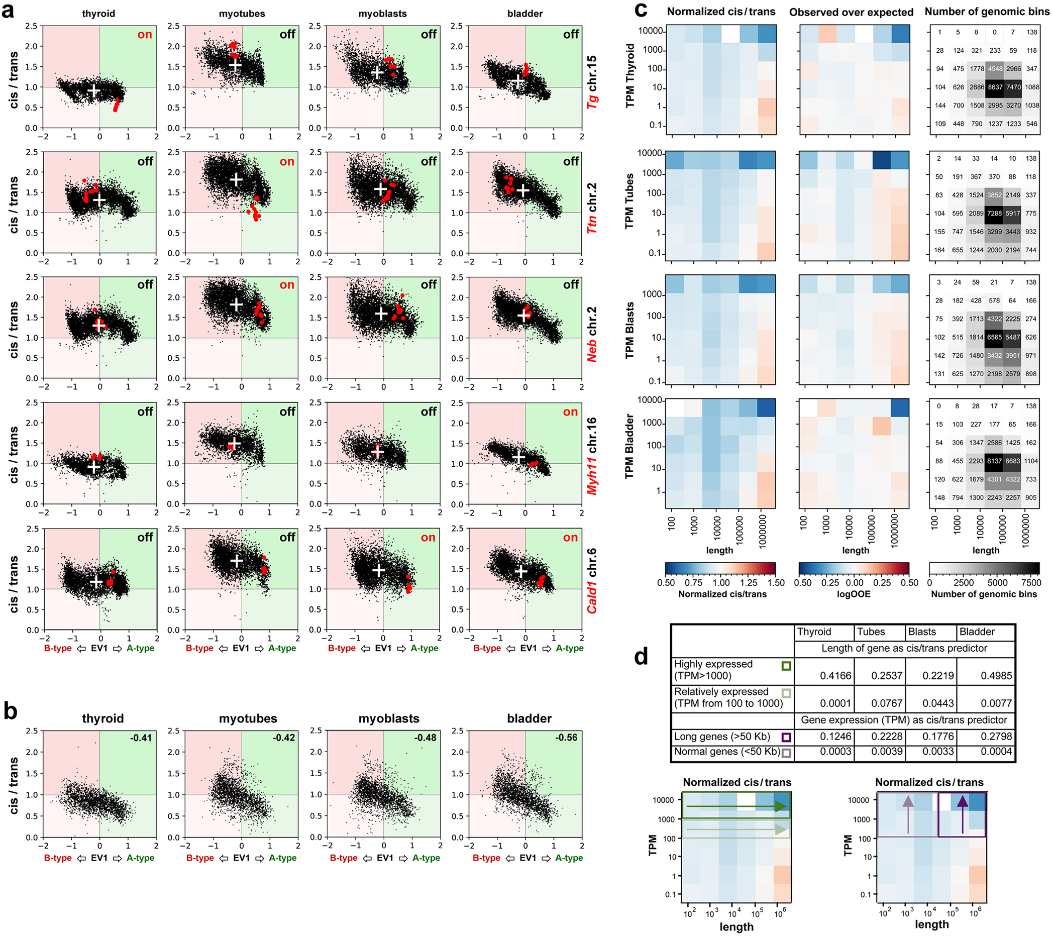
a, Cis-to-trans ratios and compartment affiliations for 5 studied genes. The scatter plots are computed from the compartment profiles and the cis-to-trans ratio profiles of the chromosomes harboring the genes at a bin size of 32 kb. Genes of interest are highlighted with red dots; the white crosses mark the chromosome means of the compartment and cis-to-trans ratio profiles. Tg, Ttn, Neb and Myh11 move from B to A compartment upon their activation; Cald1 is found in A compartment not only in myoblasts and smooth muscle, as expected, but also in thyroid and myotubes. This is in agreement with the low Cald1 expression also in thyroid samples enriched in blood vessels and in samples of myotubes that normally include up to 20% of myoblasts, as well as with localization of Cald1 in a gene-dense region of chromosome 6. Note that the Ttn and Neb genes tend to be in A-compartment, although to a lesser degree, also in myoblasts, which can be explained by the presence of cells that started their differentiation into single-cell myotubes.

b, Cis-to-trans ratios are lower in A than in B compartments for all four studied cell types. The scatter plots are computed from the genome wide compartment profile and the cis-to-trans ratio profile, both at a bin size of 1,024 kb. The Pearson correlation coefficients are indicated in the upper right corners of the scatter plots.

c, Externalization of the expressed genes from their harboring chromosomes measured by the cis-to-trans ratios as a function of gene length and expression in corresponding tissues. Left column of heatmaps: median cis-to-trans normalized by chromosome. Notice the reduction of cis-to-trans (i.e., increasing externalization) for highly transcribed genes (top rows in each heatmap) as gene length increases (moving from left to right). Similarly, cis-to-trans goes down for long genes (right-most column of each heatmap) as expression increases (going up along this column). Interestingly, lowly transcribed long genes (lower right corner) have high cis-to-trans, indicating strong internalization, but become strongly externalized as they become highly expressed (upper right corner). Middle column: median cis-to-trans ratios controlled for compartmental signal (the first eigenvector, E1). Heatmaps show the logarithm of observed median cis-to-trans ratio divided by the expected given E1 in the corresponding bin. For the expected value, all the genomic bins were separated into 20 ranges by their E1, and the median cis-totrans for each range was considered as expected. Notice that for most genes, E1 explains most of the cisto-trans ratio. However, cis-to-trans is considerably lower for extremely long and extremely highly transcribed genes (upper right corner of each heatmap). Right column: the number of genomic bins in each range of length and transcription. Notice that very few genes show high externalization.

d, Table of coefficients of determination (R2) for regression of cis-to-trans ratios of the genomic bins normalized by chromosome, in four tissues. Only the bins of expressed genes (TPM>100) are considered. Gene length is an excellent predictor of cis-to-trans ratio for genomic bins of highly expressed genes (TPM>1000, 1st row), but not for other expressed genes (TPM from 100 to 1000, 2nd row). Gene expression is a good predictor of cis-to-trans ratio for genomic bins of long genes (TPM>50 Kb, 3rd row), but not for shorter genes (TPM<50 Kb, last row). Heatmaps: visual illustration of gene subsets in this analysis.

Extended Data Fig. 9. TLs do not cause insulation at different length scales.

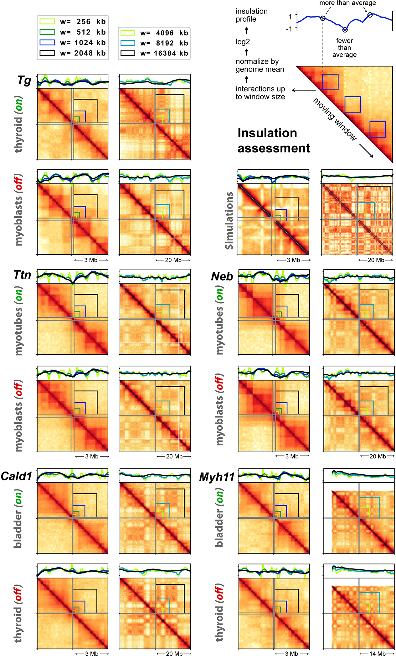
Insulation assesses Hi-C contacts spanning across a given locus up to a maximal distance w (top right insert). Contacts in a square window of size w were aggregated and the square was slid along the Hi-C diagonal. The score was normalized by its genome wide mean. Profiles show log2 of the score, such that a locus with profile value −1 has a two-fold reduced number of contacts spanning the locus up to distance w compared to the genome wide mean. Insulation scores are computed with the cooltools package (https://github.com/mirnylab/cooltools). We computed insulation profiles for Hi-C maps with a bin size of 128 kb for various window sizes from 256 kb up to ≈16 Mb. For every analyzed gene, the left and right columns show a 3 and 20 Mb Hi-C map with insulation profiles for different window sizes; the top and bottom panels show insulation profiles in expressing (on) and non-expressing (off) cells, respectively. The analysis shows little correlation between insulation and the formation of TLs: insulation profiles at the gene loci do not differ much between cell types with the gene on or off. For example, the Tg gene shows a moderate dip at scales up to ≈1Mb in both thyroids (on) and myoblasts (off), and no dip in either cell type on the larger scale. Analysis of simulated TLs (Fig. 8 and Extended data Fig. 10) confirmed that TL formation does not cause large scale insulation (bottom row).

Extended Data Fig. 10. Polymer simulation of chromosomes.

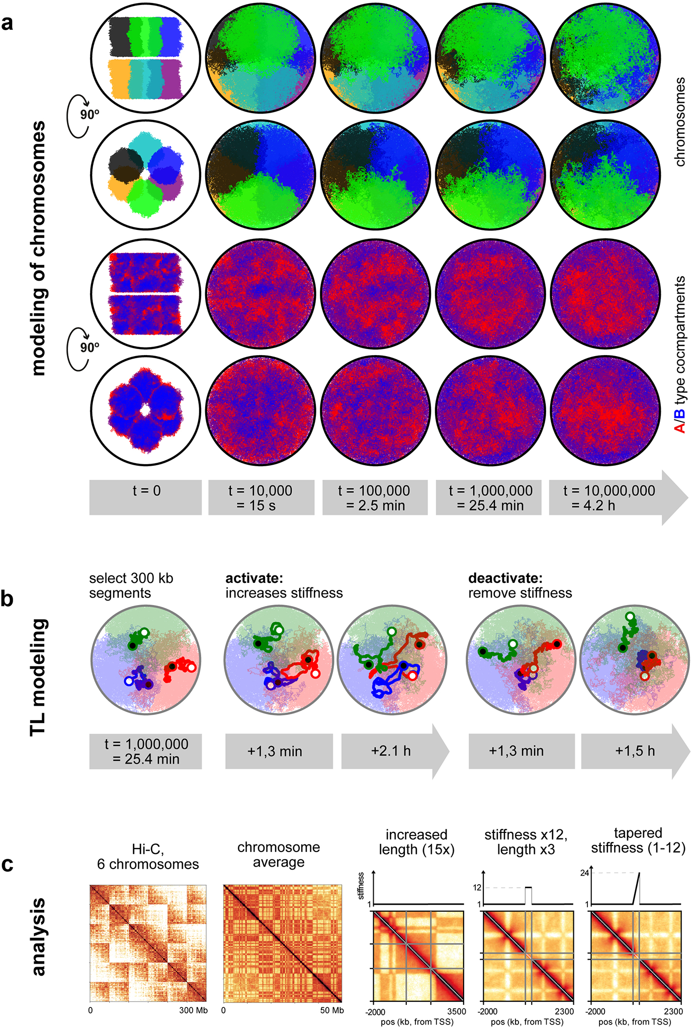
a, Six chromosomes (50 Mb each) were initiated in a mitotic-like state with unit volume density. Row 1 and 3 show top views, row 2 and 4 show side views. In rows 1 and 2 six chromosomes are differentially colored; in rows 3 and 4 compartmental segments of A and B type chromatin are differentially colored with red for A and blue for B compartments. The initial expansion is very fast (column 2). However, once the chromosomes fill the nucleus uniformly, the subsequent dynamics is very slow and chromosomes retain their territoriality (note that times increase logarithmically). Nevertheless, due to attraction of B-type chromatin to the lamina, a radial structure emerges (rows 3 and 4). b, TLs are modeled by choosing a 300 kb segment on each chromosome 25.4 minutes after expansion and increasing the stiffness of the polymer fiber. The genes quickly expand on the order of minutes and are simulated for approximately 1.5 h. The measurements of inter-flank distances and Hi-C maps are performed using configurations sampled from the second half of this time interval. When genes are deactivated by removing the excess stiffness, they collapse back to the inactive state. c, Left: Hi-C of all 6 chromosomes shows their territoriality as patches. Second-left: A Hi-C contact map averaged over all 6 chromosomes exhibits the checkerboard pattern of a typical segregation of A- and B-type chromatin. The three rightmost graphs show zoomed views of modeled genes with stiffness profiles above the maps.

REFERENCES

- 1.Andersson R & Sandelin A Determinants of enhancer and promoter activities of regulatory elements. Nat Rev Genet 21, 71–87 (2020). [DOI] [PubMed] [Google Scholar]
- 2.Cramer P Organization and regulation of gene transcription. Nature 573, 45–54 (2019). [DOI] [PubMed] [Google Scholar]
- 3.Herzel L, Straube K & Neugebauer KM Long-read sequencing of nascent RNA reveals coupling among RNA processing events. Genome Res 28, 1008–1019 (2018). [DOI] [PMC free article] [PubMed] [Google Scholar]
- 4.Feodorova Y, Falk M, Mirny LA & Solovei I Viewing Nuclear Architecture through the Eyes of Nocturnal Mammals. Trends Cell Biol 30, 276–289 (2020). [DOI] [PMC free article] [PubMed] [Google Scholar]
- 5.Solovei I, Thanisch K & Feodorova Y How to rule the nucleus: divide et impera. Curr Opin Cell Biol 40, 47–59 (2016). [DOI] [PubMed] [Google Scholar]
- 6.van Steensel B & Belmont AS Lamina-Associated Domains: Links with Chromosome Architecture, Heterochromatin, and Gene Repression. Cell 169, 780–791 (2017). [DOI] [PMC free article] [PubMed] [Google Scholar]
- 7.Macgregor HC An introduction to animal cytogenetics. (Chapman & Hall, 1993). [Google Scholar]
- 8.Bjork P & Wieslander L The Balbiani Ring Story: Synthesis, Assembly, Processing, and Transport of Specific Messenger RNA-Protein Complexes. Annu Rev Biochem 84, 65–92 (2015). [DOI] [PubMed] [Google Scholar]
- 9.Chakalova L & Fraser P Organization of transcription. Cold Spring Harb Perspect Biol 2, a000729 (2010). [DOI] [PMC free article] [PubMed] [Google Scholar]
- 10.Osborne CS et al. Active genes dynamically colocalize to shared sites of ongoing transcription. Nat Genet 36, 1065–1071 (2004). [DOI] [PubMed] [Google Scholar]
- 11.Schoenfelder S et al. Preferential associations between co-regulated genes reveal a transcriptional interactome in erythroid cells. Nat Genet 42, 53–61 (2010). [DOI] [PMC free article] [PubMed] [Google Scholar]
- 12.Cook PR The organization of replication and transcription. Science 284, 1790–1795 (1999). [DOI] [PubMed] [Google Scholar]
- 13.Papantonis A & Cook PR Transcription factories: genome organization and gene regulation. Chem Rev 113, 8683–8705 (2013). [DOI] [PubMed] [Google Scholar]
- 14.Mateo LJ et al. Visualizing DNA folding and RNA in embryos at single-cell resolution. Nature 568, 49–54 (2019). [DOI] [PMC free article] [PubMed] [Google Scholar]
- 15.Nora EP et al. Spatial partitioning of the regulatory landscape of the X-inactivation centre. Nature 485, 381–385 (2012). [DOI] [PMC free article] [PubMed] [Google Scholar]
- 16.Rodermund L et al. Time-resolved structured illumination microscopy reveals key principles of Xist RNA spreading. Science 372 (2021). [DOI] [PubMed] [Google Scholar]
- 17.Morgan GT Imaging the dynamics of transcription loops in living chromosomes. Chromosoma (2018). [DOI] [PMC free article] [PubMed] [Google Scholar]
- 18.Schermelleh L, Heintzmann R & Leonhardt H A guide to super-resolution fluorescence microscopy. J Cell Biol 190, 165–175 (2010). [DOI] [PMC free article] [PubMed] [Google Scholar]
- 19.Jjingo D, Huda A, Gundapuneni M, Marino-Ramirez L & Jordan IK Effect of the transposable element environment of human genes on gene length and expression. Genome Biol Evol 3, 259–271 (2011). [DOI] [PMC free article] [PubMed] [Google Scholar]
- 20.Hutchison N Lampbrush chromosomes of the chicken, Gallus domesticus. J Cell Biol 105, 1493–1500 (1987). [DOI] [PMC free article] [PubMed] [Google Scholar]
- 21.Miller OL & Beatty BR Visualization of nuclear genes. Science 164, 955–957 (1969). [DOI] [PubMed] [Google Scholar]
- 22.Kaufmann R, Cremer C & Gall JG Superresolution imaging of transcription units on newt lampbrush chromosomes. Chromosome Res 20, 1009–1015 (2012). [DOI] [PMC free article] [PubMed] [Google Scholar]
- 23.Carmo-Fonseca M & Kirchhausen T The timing of pre-mRNA splicing visualized in real-time. Nucleus 5, 11–14 (2014). [DOI] [PMC free article] [PubMed] [Google Scholar]
- 24.Ansari A & Hampsey M A role for the CPF 3’-end processing machinery in RNAP II-dependent gene looping. Genes Dev 19, 2969–2978 (2005). [DOI] [PMC free article] [PubMed] [Google Scholar]
- 25.Larsson AJM et al. Genomic encoding of transcriptional burst kinetics. Nature (2019). [DOI] [PMC free article] [PubMed] [Google Scholar]
- 26.Tantale K et al. A single-molecule view of transcription reveals convoys of RNA polymerases and multi-scale bursting. Nat Commun 7, 12248 (2016). [DOI] [PMC free article] [PubMed] [Google Scholar]
- 27.Chavez A et al. Highly efficient Cas9-mediated transcriptional programming. Nat Methods 12, 326–328 (2015). [DOI] [PMC free article] [PubMed] [Google Scholar]
- 28.Bensaude O Inhibiting eukaryotic transcription: Which compound to choose? How to evaluate its activity? Transcription 2, 103–108 (2011). [DOI] [PMC free article] [PubMed] [Google Scholar]
- 29.Mahy NL, Perry PE, Gilchrist S, Baldock RA & Bickmore WA Spatial organization of active and inactive genes and noncoding DNA within chromosome territories. J Cell Biol 157, 579–589 (2002). [DOI] [PMC free article] [PubMed] [Google Scholar]
- 30.Brown JM et al. Association between active genes occurs at nuclear speckles and is modulated by chromatin environment. J Cell Biol 182, 1083–1097 (2008). [DOI] [PMC free article] [PubMed] [Google Scholar]
- 31.Chambeyron S, Da Silva NR, Lawson KA & Bickmore WA Nuclear re-organisation of the Hoxb complex during mouse embryonic development. Development 132, 2215–2223 (2005). [DOI] [PubMed] [Google Scholar]
- 32.Mahy NL, Perry PE & Bickmore WA Gene density and transcription influence the localization of chromatin outside of chromosome territories detectable by FISH. J Cell Biol 159, 753–763 (2002). [DOI] [PMC free article] [PubMed] [Google Scholar]
- 33.Volpi EV et al. Large-scale chromatin organization of the major histocompatibility complex and other regions of human chromosome 6 and its response to interferon in interphase nuclei. J Cell Sci 113 ( Pt 9), 1565–1576 (2000). [DOI] [PubMed] [Google Scholar]
- 34.Williams RR, Broad S, Sheer D & Ragoussis J Subchromosomal positioning of the epidermal differentiation complex (EDC) in keratinocyte and lymphoblast interphase nuclei. Exp Cell Res 272, 163–175 (2002). [DOI] [PubMed] [Google Scholar]
- 35.Abramo K et al. A chromosome folding intermediate at the condensin-to-cohesin transition during telophase. Nat Cell Biol 21, 1393–1402 (2019). [DOI] [PMC free article] [PubMed] [Google Scholar]
- 36.Kalhor R, Tjong H, Jayathilaka N, Alber F & Chen L Genome architectures revealed by tethered chromosome conformation capture and population-based modeling. Nat Biotechnol 30, 90–98 (2012). [DOI] [PMC free article] [PubMed] [Google Scholar]
- 37.Shah S et al. Dynamics and Spatial Genomics of the Nascent Transcriptome by Intron seqFISH. Cell 174, 363–376 e316 (2018). [DOI] [PMC free article] [PubMed] [Google Scholar]
- 38.Hsieh TS et al. Resolving the 3D Landscape of Transcription-Linked Mammalian Chromatin Folding. Mol Cell (2020). [DOI] [PMC free article] [PubMed] [Google Scholar]
- 39.Banigan EJ & Mirny LA The interplay between asymmetric and symmetric DNA loop extrusion. Elife 9 (2020). [DOI] [PMC free article] [PubMed] [Google Scholar]
- 40.Brandao HB et al. RNA polymerases as moving barriers to condensin loop extrusion. Proc Natl Acad Sci U S A (2019). [DOI] [PMC free article] [PubMed] [Google Scholar]
- 41.Muller-McNicoll M & Neugebauer KM How cells get the message: dynamic assembly and function of mRNA-protein complexes. Nat Rev Genet 14, 275–287 (2013). [DOI] [PubMed] [Google Scholar]
- 42.Olins AL & Olins DE Spheroid chromatin units (v bodies). Science 183, 330–332 (1974). [DOI] [PubMed] [Google Scholar]
- 43.Liu X, Farnung L, Wigge C & Cramer P Cryo-EM structure of a mammalian RNA polymerase II elongation complex inhibited by alpha-amanitin. J Biol Chem 293, 7189–7194 (2018). [DOI] [PMC free article] [PubMed] [Google Scholar]
- 44.Paturej J, Sheiko SS, Panyukov S & Rubinstein M Molecular structure of bottlebrush polymers in melts. Sci Adv 2, e1601478 (2016). [DOI] [PMC free article] [PubMed] [Google Scholar]
- 45.Kotake Y et al. Splicing factor SF3b as a target of the antitumor natural product pladienolide. Nat Chem Biol 3, 570–575 (2007). [DOI] [PubMed] [Google Scholar]
- 46.Mirny LA & Solovei I Keeping chromatin in the loop(s). Nat Rev Mol Cell Biol (2021). [DOI] [PubMed] [Google Scholar]
- 47.Cho WK et al. Mediator and RNA polymerase II clusters associate in transcription-dependent condensates. Science 361, 412–415 (2018). [DOI] [PMC free article] [PubMed] [Google Scholar]
- 48.Guo YE et al. Pol II phosphorylation regulates a switch between transcriptional and splicing condensates. Nature 572, 543–548 (2019). [DOI] [PMC free article] [PubMed] [Google Scholar]
- 49.Hnisz D, Shrinivas K, Young RA, Chakraborty AK & Sharp PA A Phase Separation Model for Transcriptional Control. Cell 169, 13–23 (2017). [DOI] [PMC free article] [PubMed] [Google Scholar]
- 50.Cisse II et al. Real-time dynamics of RNA polymerase II clustering in live human cells. Science 341, 664–667 (2013). [DOI] [PubMed] [Google Scholar]
- 51.Henninger JE et al. RNA-Mediated Feedback Control of Transcriptional Condensates. Cell 184, 207–225 e224 (2021). [DOI] [PMC free article] [PubMed] [Google Scholar]
- 52.Hampsey M, Singh BN, Ansari A, Laine JP & Krishnamurthy S Control of eukaryotic gene expression: gene loops and transcriptional memory. Adv Enzyme Regul 51, 118–125 (2011). [DOI] [PMC free article] [PubMed] [Google Scholar]
- 53.Martin M, Cho J, Cesare AJ, Griffith JD & Attardi G Termination factor-mediated DNA loop between termination and initiation sites drives mitochondrial rRNA synthesis. Cell 123, 1227–1240 (2005). [DOI] [PubMed] [Google Scholar]
- 54.Singh BN & Hampsey M A transcription-independent role for TFIIB in gene looping. Mol Cell 27, 806–816 (2007). [DOI] [PubMed] [Google Scholar]
- 55.Lee K, Hsiung CC, Huang P, Raj A & Blobel GA Dynamic enhancer-gene body contacts during transcription elongation. Genes Dev 29, 1992–1997 (2015). [DOI] [PMC free article] [PubMed] [Google Scholar]
- 56.Zheng M et al. Multiplex chromatin interactions with single-molecule precision. Nature (2019). [DOI] [PMC free article] [PubMed] [Google Scholar]
- 57.Cremer T & Cremer M Chromosome territories. Cold Spring Harb Perspect Biol 2, a003889 (2010). [DOI] [PMC free article] [PubMed] [Google Scholar]
- 58.Keizer VIP et al. Live-cell micromanipulation of a genomic locus reveals interphase chromatin mechanics. BioRxiv 10.1101/2021.04.20.439763 (2021). [DOI] [PubMed] [Google Scholar]
- 59.Khanna N, Zhang Y, Lucas JS, Dudko OK & Murre C Chromosome dynamics near the sol-gel phase transition dictate the timing of remote genomic interactions. Nat Commun 10, 2771 (2019). [DOI] [PMC free article] [PubMed] [Google Scholar]
- 60.Strickfaden H et al. Condensed Chromatin Behaves like a Solid on the Mesoscale In Vitro and in Living Cells. Cell 183, 1772–1784 e1713 (2020). [DOI] [PubMed] [Google Scholar]
- 61.Bagnoli JW et al. Sensitive and powerful single-cell RNA sequencing using mcSCRB-seq. Nat Commun 9, 2937 (2018). [DOI] [PMC free article] [PubMed] [Google Scholar]
- 62.Ziegenhain C et al. Comparative Analysis of Single-Cell RNA Sequencing Methods. Mol Cell 65, 631–643 e634 (2017). [DOI] [PubMed] [Google Scholar]
- 63.Parekh S, Ziegenhain C, Vieth B, Enard W & Hellmann I zUMIs - A fast and flexible pipeline to process RNA sequencing data with UMIs. Gigascience 7 (2018). [DOI] [PMC free article] [PubMed] [Google Scholar]
- 64.Rau A, Gallopin M, Celeux G & Jaffrezic F Data-based filtering for replicated high-throughput transcriptome sequencing experiments. Bioinformatics 29, 2146–2152 (2013). [DOI] [PMC free article] [PubMed] [Google Scholar]
- 65.Mali P et al. RNA-guided human genome engineering via Cas9. Science 339, 823–826 (2013). [DOI] [PMC free article] [PubMed] [Google Scholar]
- 66.Link S et al. PWWP2A binds distinct chromatin moieties and interacts with an MTA1-specific core NuRD complex. Nat Commun 9, 4300 (2018). [DOI] [PMC free article] [PubMed] [Google Scholar]
- 67.Punzeler S et al. Multivalent binding of PWWP2A to H2A.Z regulates mitosis and neural crest differentiation. EMBO J 36, 2263–2279 (2017). [DOI] [PMC free article] [PubMed] [Google Scholar]
- 68.Belaghzal H, Dekker J & Gibcus JH Hi-C 2.0: An optimized Hi-C procedure for high-resolution genome-wide mapping of chromosome conformation. Methods 123, 56–65 (2017). [DOI] [PMC free article] [PubMed] [Google Scholar]
- 69.Abdennur N & Mirny LA Cooler: scalable storage for Hi-C data and other genomically labeled arrays. Bioinformatics 36, 311–316 (2020). [DOI] [PMC free article] [PubMed] [Google Scholar]
- 70.Imakaev M et al. Iterative correction of Hi-C data reveals hallmarks of chromosome organization. Nat Methods 9, 999–1003 (2012). [DOI] [PMC free article] [PubMed] [Google Scholar]
- 71.Cremer M et al. Multicolor 3D fluorescence in situ hybridization for imaging interphase chromosomes. Methods Mol Biol 463, 205–239 (2008). [DOI] [PubMed] [Google Scholar]
- 72.Kishi JY et al. SABER amplifies FISH: enhanced multiplexed imaging of RNA and DNA in cells and tissues. Nature Methods 16, 533–544 (2019). [DOI] [PMC free article] [PubMed] [Google Scholar]
- 73.Kishi JY, Schaus TE, Gopalkrishnan N, Xuan F & Yin P Programmable autonomous synthesis of single-stranded DNA. Nat Chem 10, 155–164 (2018). [DOI] [PMC free article] [PubMed] [Google Scholar]
- 74.Bienko M et al. A versatile genome-scale PCR-based pipeline for high-definition DNA FISH. Nat Methods 10, 122–124 (2013). [DOI] [PMC free article] [PubMed] [Google Scholar]
- 75.Solovei I & Cremer M 3D-FISH on cultured cells combined with immunostaining, in Methods Mol Biol, Vol. 659 117–126 (2010). [DOI] [PubMed] [Google Scholar]
- 76.Solovei I et al. FISH on three-dimensionally preserved nuclei, in FISH: a practical approach. (eds. Beatty B, Mai S & Squire J) 119–157 (Oxford University press, 2002). [Google Scholar]
- 77.Solovei I Fluorescence in situ hybridization (FISH) on tissue cryosections, in Methods Mol Biol, Vol. 659 71–82 (2010). [DOI] [PubMed] [Google Scholar]
- 78.Eberhart A et al. Epigenetics of eu- and heterochromatin in inverted and conventional nuclei from mouse retina. Chromosome Res 21, 535–554 (2013). [DOI] [PubMed] [Google Scholar]
- 79.Eberhart A, Kimura H, Leonhardt H, Joffe B & Solovei I Reliable detection of epigenetic histone marks and nuclear proteins in tissue cryosections. Chromosome Res 20, 849–858 (2012). [DOI] [PubMed] [Google Scholar]
- 80.Solovei I et al. LBR and lamin A/C sequentially tether peripheral heterochromatin and inversely regulate differentiation. Cell 152, 584–598 (2013). [DOI] [PubMed] [Google Scholar]
- 81.Walter J et al. Towards many colors in FISH on 3D-preserved interphase nuclei. Cytogenet Genome Res 114, 367–378 (2006). [DOI] [PubMed] [Google Scholar]
- 82.Bystricky K, Heun P, Gehlen L, Langowski J & Gasser SM Long-range compaction and flexibility of interphase chromatin in budding yeast analyzed by high-resolution imaging techniques. Proc Natl Acad Sci U S A 101, 16495–16500 (2004). [DOI] [PMC free article] [PubMed] [Google Scholar]
- 83.Dekker J, Rippe K, Dekker M & Kleckner N Capturing chromosome conformation. Science 295, 1306–1311 (2002). [DOI] [PubMed] [Google Scholar]
- 84.Rippe K Making contacts on a nucleic acid polymer. Trends Biochem Sci 26, 733–740 (2001). [DOI] [PubMed] [Google Scholar]
- 85.Ou HD et al. ChromEMT: Visualizing 3D chromatin structure and compaction in interphase and mitotic cells. Science 357 (2017). [DOI] [PMC free article] [PubMed] [Google Scholar]
- 86.Hajjoul H et al. High-throughput chromatin motion tracking in living yeast reveals the flexibility of the fiber throughout the genome. Genome Res 23, 1829–1838 (2013). [DOI] [PMC free article] [PubMed] [Google Scholar]
- 87.Lucas JS, Zhang Y, Dudko OK & Murre C 3D trajectories adopted by coding and regulatory DNA elements: first-passage times for genomic interactions. Cell 158, 339–352 (2014). [DOI] [PMC free article] [PubMed] [Google Scholar]
- 88.Nuebler J, Fudenberg G, Imakaev M, Abdennur N & Mirny LA Chromatin organization by an interplay of loop extrusion and compartmental segregation. Proc Natl Acad Sci U S A 115, E6697–E6706 (2018). [DOI] [PMC free article] [PubMed] [Google Scholar]
Associated Data
This section collects any data citations, data availability statements, or supplementary materials included in this article.
Supplementary Materials
Data Availability Statement