High-speed super-resolution imaging of rotationally symmetric structures using SPEED microscopy and 2D-to-3D transformation

Abstract

Various super-resolution imaging techniques have been developed to break the diffraction-limited resolution of light microscopy. However, it still remains challenging to obtain three-dimensional (3D) super-resolution information of structures and dynamic processes in live cells at high speed. We recently developed high-speed single-point edge-excitation sub-diffraction (SPEED) microscopy and its two-dimensional (2D)-to-3D transformation algorithm to provide an effective approach to achieving 3D sub-diffraction-limit information in subcellular structures and organelles that have rotational symmetry. In contrast to most other 3D super-resolution microscopy or 3D particle-tracking microscopy approaches, SPEED microscopy does not depend on complex optical components and can be implemented onto a standard inverted epifluorescence microscope. SPEED microscopy is specifically designed to obtain 2D spatial locations of individual immobile or moving fluorescent molecules inside sub-micrometer biological channels or cavities at high spatiotemporal resolution. After data collection, post-localization 2D-to-3D transformation is applied to obtain 3D superresolution structural and dynamic information. The complete protocol, including cell culture and sample preparation (6–7 d), SPEED imaging (4–5 h), data analysis and validation through simulation (5–13 h), takes ~9 d to complete.

Introduction

For many years, scientists have been motivated to improve the imaging resolution of light microscopy to gain a foundational understanding of subcellular structure and dynamical processes under physiological conditions. However, this pursuit is severely hampered by the physical limitations of light that govern the ability of a microscope to resolve an object. Since stated by Ernst Abbe in 1873¹, the resolution of conventional light microscopy has been thought to be limited at ~200 nm owing to light diffraction. Abbe’s diffraction limit is defined as $d=\frac{\lambda }{2NA}$, where d is the diffraction limit, λ is the wavelength and NA is the numerical aperture of the microscope^2,3. Currently, super-resolution light microscopy techniques have broken this limitation and brought sub-diffraction-limit images into our focus⁴. Although various approaches have been suggested, the widely applied techniques could generally fall into two broad categories. The first category comprises the single-molecule localization algorithm-based super-resolution techniques, such as stochastic optical reconstruction microscopy (STORM)⁵ and photoactivated localization microscopy (PALM)⁶, and DNA-based point accumulation for imaging in nanoscale topography (DNA-PAINT)⁷, which use mathematical functions to localize the centroids of individual fluorophores and then reconstitute these centroids to form superresolution images. The second category comprises patterned optics-based super-resolution techniques, which collect sub-diffraction-limit information from high-frequency spatial signal or nonlinear optical response of fluorophores in samples, including structured illumination microscopy (SIM)⁸ and stimulated emission depletion (STED)⁹.

In STORM, PALM and DNA-PAINT, the success of super-resolution microscopy imaging depends on the accurate localization of individual fluorescent molecules. This relies on the separation of fluorescent emitters in such a manner that the point spread function (PSF) of each emitter ideally does not overlap. To achieve the spatially well-separated PSFs, emitters are temporally separated by limiting the number of simultaneously emitting particles^5,10,11. This is originally accomplished in PALM through the use of photoactivatable proteins, in STORM through the use of photoswitchable dyes and then in DNA-PAINT through transient binding between fluorophores and molecules of interest. These single-molecule localization approaches require the capture and compilation of a few thousand images to generate super-resolution images with a lateral spatial precision of ~5–20 nm. Later, PSF engineering was applied to these localization techniques, enabling the derivation of axial, or 3D, information due to induced changes in the PSF^12,13. Traditionally, these time-intensive approaches have been successfully applied to fixed cells^6,14,15. Notably, single-particle tracking PALM (sptPALM) was developed by combining single-particle tracking with PALM¹⁶. This enables researchers to observe the diffusion of highly dense particles on membranes¹⁶, the trafficking and molecular interactions of membrane bound receptors¹⁷ and the dynamics of intraflagellar transport proteins¹⁸. This approach is capable of providing 2D lateral spatial information of high-density single-particle dynamics in cellular processes occurring slower than ~50 ms^16,19 (Table 1).

Table 1 |.

Key features of the predominant super-resolution microscopy approaches

Method	Common abbreviations	Comments	3D capable	Resolution In nm	Temporal resolution	Live-cell Imaging or single-particle tracking	Ref.
Localization	Pointillism, PALM, STORM	Use photoswitchable fluorophores or photoactivatable proteins. Reconstitution of a high-quality image requires a large amount of localized molecules.	Yes,. Localization algorithms use PSF shape to derive z information.	-20 (x,y) -50 (z)	10–100 s (PALM) -3 s (STORM)	Live-cell imaging is possible.	5,6,8,10–15,68–77
	DNA-PAINT	Use DNA nanotechnology to set up a programmable target-probe binding. ‘Stochastic blinking’ is achieved by transient binding between the probe and target.	Yes. Localization algorithms use PSF shape to derive z information	-5 (x,y) -24 (z)	200–300 ms	Limited to fixed specimen, but application on live-cell surface is possible.	7,66,67,78–84
Structure Illumination	3D-SIM, SIM, PEM, LMEM, HELM, Lattice Microscopy	Applies excitation patterns in different orientations and then uses post-processing to achieve a two-fold lateral localization increase. Several images are required to achieve super resolution.	Yes. 3D-SIM uses a third laser to achieve a two-fold axial localization increase.	-100 (x,y) -400 (z)	130–1,500 ms	Live-cell imaging is possible	20–23,85–88
Stimulated emission depletion	STED	Changes the effective PSF of the excitation laser by using a second STED laser to suppress fluorescence.	Yes, but requires a 4Pi configuration to improve the axial spatial resolution.	-20 (x,y) -35 (z)	-35 ms -12.5 ms (constrained field of view)	Live-cell imaging is possible	9,25–35,47,63,89,90
Single-particle localization	sptPALM	Combines PALM with live-cell single-particle tracking.	No	-50 (x,y)	-50 ms	Live-cell single-particle tracking	16–19,91,92
Single-particle localization	SPEED	Localizes a fluorescently tagged rotationally symmetric structure and tracks fluorescent particles as they move through the structure.	Yes. Virtual 3D via a 2D-to-3D transformation algorithm	-10–20 (x,y)	-0.4 ms for tracking -1–3 s for structure	Live-cell single-particle tracking	38,42,44–46,93

Included here is a non-exhaustive list of super-resolution microscopy techniques, including suitability for live-cell imaging, 3D capability and the published temporal, lateral and axial localization precisions.

SIM microscopy is able to generate super-resolution images by passing laser light through movable optical grating, which then projects onto the sample in a series of sinusoidal striped patterns of high spatial frequency^3,20,21. A series of images are captured with the grating in different configurations, generating novel moiré information. The images are then overlaid and analyzed with computer algorithms to produce an image of the underlying structure. This approach provides a two-fold increase in lateral localization precision over the classical diffraction limit²⁰. To derive 3D information, multiple optical sections are captured along the z axis and combined into a 3D composite. This adaptation is made possible by the addition of a third laser beam, thereby inducing three-beam interference^22,23. The addition of the third beam enables 3D-SIM to provide a z-stack of images with an axial localization precision of ~400 nm²³, which represents approximately a two-fold enhancement when compared to conventional fluorescence imaging techniques (Table 1).

STED microscopy controls the de-excitation of previously excited fluorophores with the addition of a second, doughnut-shaped STED laser beam. Fluorophores surrounding the center of the scanning spot—the zero-intensity center of the STED beam—are illuminated with the STED beam and are, thereby, pushed into the ground state. This causes these fluorophores to emit light at the wavelength of the STED beam. Fluorescence from the scanning spot is then spectrally separated and detected, producing an image with a lateral localization precision of ~20–50 nm^3,9,24–28 (Table 1). In an effort to improve 3D localization in STED microscopy, two approaches have been employed to limit the axial PSF, thereby improving z localization. The first is technically difficult and requires the combination of STED with 4Pi microscopy to create 4Pi-STED microscopy. This approach has demonstrated experimental axial localizations of ~50 nm^29–31. The second technique involves engineering the PSF by superimposing two incoherent STED beams. One produces the standard doughnut-shaped STED beam, whereas the second produces a bottle-shaped focus that functions as a ‘z doughnut’ and, thereby, constrains axial fluorescence³². This system has been experimentally demonstrated to provide axial resolution of ~35 nm³³ (Table 1). This approach provides impressive axial resolution, but, owing to the physical characteristics of STED microscopy, live-cell imaging might require a reduction in the STED beam power and therefore a potential reduction in resolution^25,34–36, whereas in MINFLUX microscopy the doughnut-shaped laser from STED microscopy was directly used to excite photoswitchable emitters in a manner similar to PALM/STORM. MINFLUX obtains high spatial localization precision through localizing the emitter with a local intensity minimum of excitation light. Moreover, recently, the usage of the 3D doughnut-shaped excitation lasers expanded MINFLUX to achieve multicolor nanometer 3D resolutions³⁷.

To complement these approaches and achieve 3D super-resolution imaging of subcellular structure and fast dynamic processes in live cells, we developed SPEED microscopy and a 2D-to-3D transformation algorithm. SPEED microscopy falls within the category of single-molecule localization microcopy techniques and is mediated by an inclined illumination volume in the focal plane (Fig. 1a). It is specifically designed to track and record 2D spatial locations of fast-moving fluorescent molecules inside sub-micrometer biological channels or cavities with rotational symmetry (Fig. 1b) at high spatiotemporal resolutions of ≤10–20 nm and 0.4 ms (Table 1)^33–39. The post-localization 2D-to-3D transformation is then applied to obtain 3D super-resolution structural and dynamic information from the recorded 2D single-molecule trajectories and spatial distributions (Fig. 2).

Fig. 1 |. A schematic of excitation optical paths for both vertical and inclined illumination.

a, Schematic of the microscope setup for both the inclined and the vertical illumination in SPEED microscopy. A 488-nm (blue) and a 568-nm (green) laser are directed into the objective in vertical illumination or offset so that the lasers pass through the focal plane at an angle of θ₃. The inset depicts a diagram of the edge excitation optics. The refractive angle (θ_i) at the interface of two different mediums with different refractive indexes (n_i). The θ₃ depends on the focal length of the objective (a), the refractive indexes of the different mediums in the optical path and the distance (d) between the center and edge excitation beams. The relationship between θ₃ and d follows the equation: $d=a*\tan \left[{\sin }^{-1}\left(\frac{n_{cell}}{n_{oil}}\sin {\theta }_3\right)\right]$, where a = 300 μm, n_cell = 1.33 and n_oil = 1.516. For example, to obtain θ_{3 =} 45°, d needs to be 237 μm. b, An illustration of a molecule traveling in three dimensions as it passes through an NPC. A 2D projection of the same pathway is depicted in the lower panel. c, An illustration of the effect of the optical chopper on laser intensity. The chopper is calibrated to be open for 1/10 of frames captured.

Fig. 2 |. 3D information derived from 2D single-molecule data using a 2D-to-3D transformation.

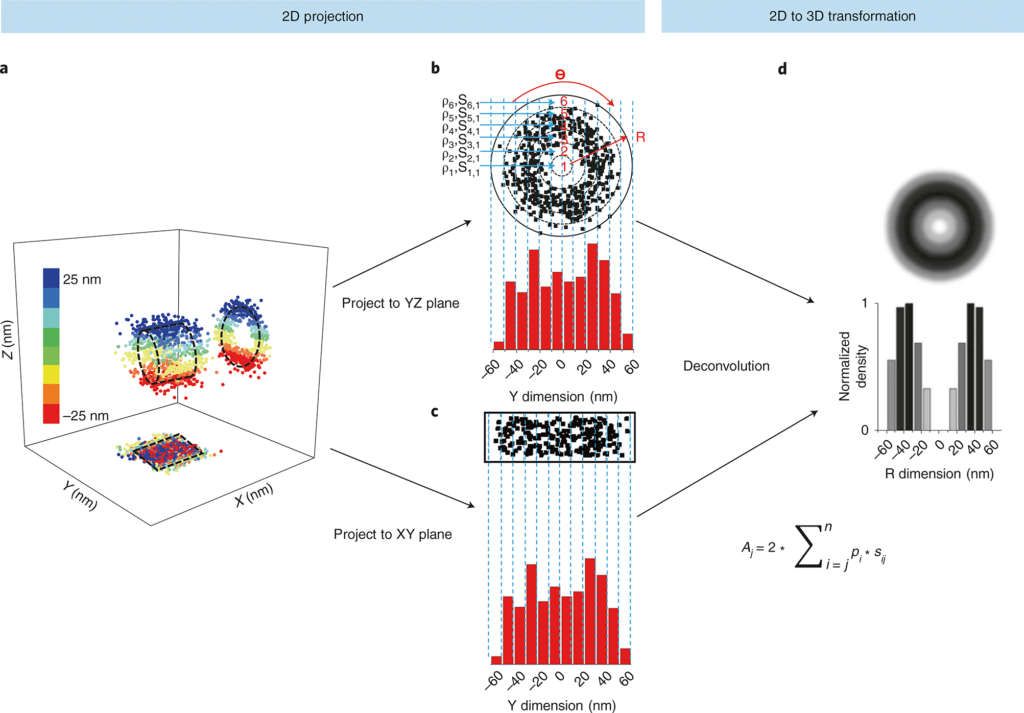
a, Simulated single-molecule data in the x, y and z dimensions in a rotationally symmetric cylinder with a radius of 25 nm. Below the cylinder is the 2D projection onto the x,y plane. A projection of an axial slice is shown in the R,θ dimensions. b, Single-molecule data from the y,z plane are projected onto an area matrix. A histogram is generated from the y,z plane with a bin size of 10 nm. c, The projection of single-molecule data onto the x,y plane as well as a histogram of the x,y plane with a 10-nm bin value. d, A representative radial density map of the 2D projections with a corresponding histogram with a 10-nm bin size. The equation for 2D-to-3D transformation is also shown here. Given the high number of randomly distributed molecules in the rotationally symmetric cylinder, the spatial density of locations (ρ_i) in each sub-region (s_(i,j)) between two neighboring rings will be rotationally symmetrical and uniform. These locations can be further projected into one dimension along the y dimension. The locations along the y dimension can be clustered in a histogram with j columns. The total number of locations in each column (A_(i,j)) is equal to $2*{\sum }_{i=j}^n{\rho }_i*s_{(i,j)}$.

Development of the approach

We originally developed SPEED microscopy by modifying an existing inverted epifluorescence microscope by introducing an inclined diffraction limit spot illumination volume in the focal plane (Fig. 1a). The inclined illumination pattern integrates some illumination features of laser scanning confocal microscopy (LSCM) as well as total internal reflection fluorescence (TIRF) microscopy. Several modifications have been made to the epifluorescence microscope to allow for SPEED microscopy^38,39. (i) Different from LSCM, SPEED microscopy uses a CCD camera instead of a photomultiplier tube (PMT) as the detector, and there is no pinhole in front of the detector, which enables the detector to directly record spatial information and collect photons from a larger area. (ii) After removing some expansion and alignment optics in an existing inverted epifluorescence microscope (see more details in the ‘SPEED microcopy’ section), an excitation laser beam is guided to the rear aperture of objective and shifted off the central axis of the objective to form an inclined laser beam focused at the focal plane instead of the total internal reflection characteristic of TIRF microscopy (Fig. 1a). The inclined laser beam generates a smaller effective illumination volume in the axial direction of the objective and partially suppresses out-of-focus background fluorescence. Also, the edge excitation avoids auto-fluorescence from the center of the objective. All of these measures help to obtain a higher signal-to-noise ratio (SNR) for single-molecule localization compared to epifluorescence or confocal imaging, which have significant out-of-focus fluorescence. (iii) High laser power density can be generated at the focal plane even with a low continuous-wave laser power, which allows a high number of photons from the fluorophores to be obtained in a short time period. (iv) The pinpointed illumination pattern of SPEED microscopy greatly reduces photobleaching and phototoxic effects in live samples. These effects are further reduced by adapting an optical chopper to create an on/off operational mode with the off-time that is ten-fold longer than the on-time (Fig. 1c). (v) The small illumination volume of SPEED microscopy allows the imaging of single molecules within a small pixel area of the CCD camera, resulting in a fast detection speed (up to 5,000 frames per second; Fig. 1b). The high detection speed also minimizes the localization error caused by movement of single particles, enabling us to obtain a localization precision of ≤10–20 nm for moving molecules in live cells.

The above modifications allow SPEED microscopy to achieve 2D single-molecule localization information of fast dynamics occurring in subcellular structures in cells. After data acquisition, post-localization 2D-to-3D transformation is applied to obtain 3D sub-diffraction-limit structural and dynamic information from the recorded 2D information. The 2D spatial information acquired from SPEED microscopy is a projection of the corresponding actual 3D spatial information in a lateral or x, y plane (Fig. 2a). The actual 3D spatial information can be shown in a cylindrical coordinate system (x, θ, r) (Fig. 2a). In a rotational symmetric structure, the distribution of the single molecules of interest in the θ dimension is considered to be constant at each (x, r). Thus, the 3D spatial information can be described in a simplified cylindrical coordinate system (x, r). The Cartesian coordinates (x,y) of 2D spatial information are converted to simplified cylindrical coordinates (x, r), enabling us to estimate 3D spatial information in a rotational symmetric structure (Fig. 2b–d). In summary, the combination of SPEED microscopy and its subsequent 2D-to-3D transformation allows us to obtain 3D sub-diffraction-limit information of fast dynamical processes within a rotationally symmetric subcellular structure.

Overview of the procedure

The primary purpose of this protocol is to assist both novice and expert users in obtaining SPEED microscopy data in vitro and in vivo as well as 3D information via our 2D-to-3D transformation algorithm. Our protocol is based on our previous studies^38–46, and the work flow is illustrated in Fig. 5. The procedure consists of five major sections: sample preparation (Steps 1–4), high-speed SPEED microscopy experiment (Steps 5–10), 2D data analysis (Steps 11–21), 2D-to-3D transformation (Steps 22–40) and validation by simulations (Steps 41–44).

Fig. 5 |. Schematic workflow for SPEED microscopy.

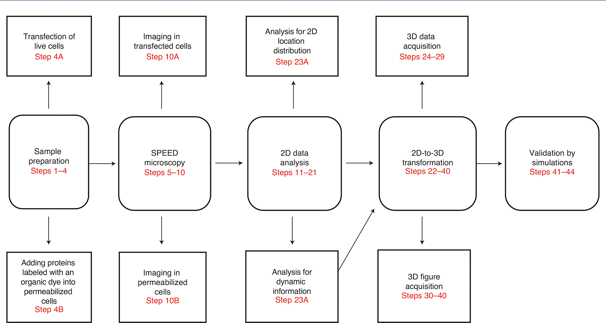
The schematic shows the five major experimental stages, including specific steps and customizations for different experiments.

The sample preparation procedures is split into two subsections: preparation for in vivo imaging (Steps 1–4 A) and preparation for in vitro imaging (Steps 1–4 B). Each of these subsections provides step-by-step instructions for fluorescence labeling and cell preparation. We then illustrate how to perform SPEED microscopy experiments, including detailed procedures for inclined-illumination and vertical-illumination setups. To achieve sufficiently high localization precision and temporal resolution (≤10–20 nm and ≤2 ms), it is particularly critical to adjust the SPEED microscope depending on specific experimental conditions (Steps 5–10). We next explain 2D data analysis for acquiring two types of information contained in the raw SPEED microscopy data—specifically, dynamic and structural information analysis (Steps 11–21). Furthermore, the 2D-to-3D transformation is described in two stages: recovery of 3D data and acquisition of 3D figures (Steps 22–40). Lastly, we explain how to validate the 3D results derived from the 2D data using simulations, including reproducibility calculation (Steps 41–44).

Advantages and limitations of the approach

Our virtual 3D super-resolution imaging technique offers several advantages compared to other 3D super-resolution microscopy approaches. First, SPEED microscopy can be used to simultaneously record both fast dynamics and sub-micrometer subcellular structural information in three dimensions with high spatial and temporal resolution (Figs. 3 and 4). Second, SPEED microscopy benefits from a less complicated sample preparation than other single-molecule localization microscopy approaches, as no specialized fluorophores are required. Furthermore, SPEED microscopy can be widely used in live cells because of its on–off pinpointed illumination pattern with low phototoxic effects and low out-of-focus background fluorescence. Taken together, this makes SPEED microscopy an ideal approach for live-cell imaging.

Fig. 3 |. Representative data from SPEED microscopy experiments.

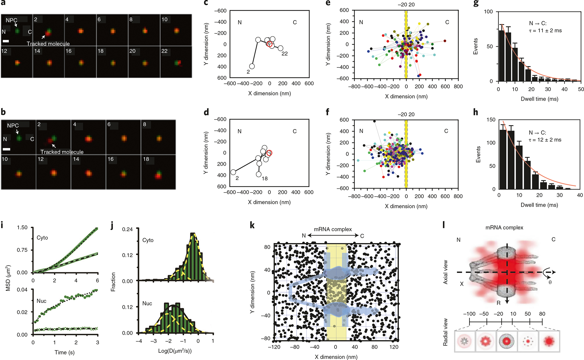
a,b, 2D single-molecular movies tracking molecules of interest around an NPC. A series of 2D locations of mRNA-mCherry (red spots) were captured by SPEED microscopy as they transported through the NPC (green spot). Numbers denote time in milliseconds. The scale bar represents 1 μm. a and b are representative of successful nuclear transport and abortive nuclear transport, respectively. The fluorescent spots of single mRNA and NPC in a series of images were fitted via a 2D Gaussian function, yielding the 2D spatial trajectory of mRNA (c,d). A 2D spatial trajectory of mRNA (black circle) transporting through the NPC (red circle) (c,d). c and d show representative trajectories for successful nuclear transport and abortive nuclear transport of mRNA, respectively. e, Superimposed single-molecule trajectories of successful mRNA export events. The central region of the NPC (221220 to 20 nm) is highlighted in yellow. C, cytoplasm; N, nucleoplasm. f, Superimposed single-molecule trajectories of abortive mRNA export events. The central region of the NPC (−20 to 20 nm) is highlighted in yellow. C, cytoplasm; N, nucleoplasm. g, Histogram depicting the export time distribution of successful mRNA export events. This histogram was fit with a mono-exponential decay function (red line), yielding the indicated median export time. Error bars represent SEM; n = 256 events. h, Histogram depicting the export time distribution of abortive messenger ribonucleoprotein (mRNP) export events. Error bars indicate SEM; n = 431 events. i, Representative mean-squared displacement versus time plots for two cytoplasmic (Cyto) and two nuclear (Nuc) mRNAs. The plots show cytoplasmic mRNA undergoing Brownian diffusion (open square, D = 0.108 μm²/s) and biased diffusion (filled square, D = 0.103 μm²/s), as well as nuclear mRNA that diffuse in a corralled fashion (filled circle, D = 0.025 μm²/s) or remain more or less stationary (open circle, D = 0.00043 μm²/s). j, Distribution of cytoplasmic (Cyto) and nuclear (Nuc) mRNP diffusion coefficients in HeLa cells. Diffusion coefficients were calculated from the mean squared displacement versus time plots of individual particles that were visible for at least nine consecutive frames. Cytoplasmic mRNPs distributed predominantly into two Gaussian distributions with average diffusion coefficients of ~0.49 μm²/s and ~0.05 μm²/s for the major (81%) and minor (19%) population, respectively. Distribution of nuclear mRNP diffusion coefficients was best fit with two Gaussian populations with average diffusion coefficients of 0.067 μm²/s (47%) and 0.009 μm²/s (53%), respectively. k, Experimentally determined 2D spatial locations of mRNPs in the NPC. A schematic of the NPC (light blue) is superimposed, and the central region of the NPC (−20 to 20 nm) is highlighted in yellow. C, cytoplasmic side of the NPC; N, nucleoplasmic side of the NPC. l, 3D spatial density map of mRNPs (red; deeper shade indicates higher density), generated using a 2D-to-3D transformation algorithm, is shown in both an axial and radial view superimposed on the NPC architecture (gray). Five regions with distinct spatial location distributions for mRNPs are marked with relative distances (in nm) from the centroid of the NPC. C, cytoplasmic side of the NPC; N, nucleoplasmic side of the NPC. Data were originally published in ref. ⁴⁵.

Fig. 4 |. Representatives of 3D probability density maps in three rotationally symmetric systems.

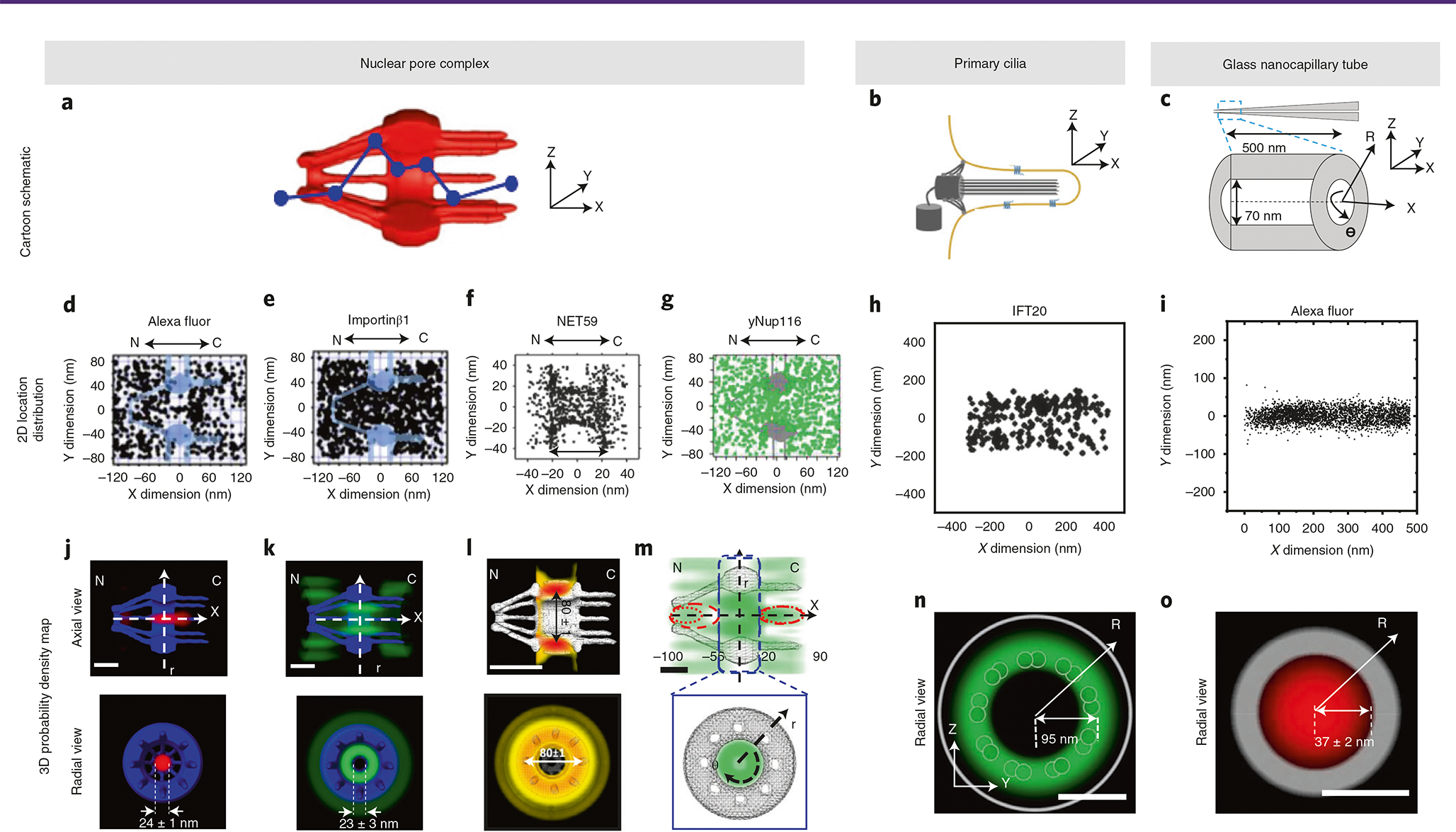
a–c, Schematic of the NPC, primary cilium and the GNC tube. d–i, 2D spatial location distribution of Alexa Fluor (small molecule), importin-β1 (nuclear transport receptor), NET59 (nuclear membrane protein) and yNup116 (FG-Nups) around NPCs. h, 2D spatial location distribution of IFT20 in primary cilia. i, 2D spatial location distribution of Alexa Fluor in a GNC tube. j–l, The 3D probability density maps for the nuclear transport route of Alexa Fluor, importin-β1 and NET59. The transport route of Alexa Fluor represents the passive diffusion pattern in NPC, whereas the transport route of importin-β1 represents the facilitated diffusion pattern in NPC. The 3D density map of NET59 represents the nuclear transport route of nuclear membrane protein. The scale bar represents 50 nm. m, The 3D probability density maps of yNup116 in NPC. This depicts the configuration of the NPC’s selectivity barrier formed by FG-Nups. The scale bar represents 50 nm. n, The 3D probability density maps for the transport route of IFT20 in primary cilia. This depicts the IFT pathway in primary cilia. The scale bar represents 100 nm. o, The 3D probability density maps for the transport route of Alexa Fluor in GNC tubes. Depicted here is a random diffusion pattern within GNC tubes. The scale bar represents 50 nm. N, nucleoplasm; C, cytoplasm. Data in a, b and c were originally published in refs. ^66,93. Data in d, e, j, k and m were originally published in ref. ⁴³. Data in f and l were originally published in ref. ⁴⁶. Data in g were originally published in ref. ⁴⁴. Data in h, i, n, and o were originally published in ref. ⁴².

However, there are a few limitations in the operation and application of the method. The first limitation is that alignment of an inclined illumination requires knowledge and skills in optics or microscopy. In the section on SPEED microscopy in Step 8, we show an alternative vertical illumination pattern used in SPEED microscopy, which reduces the technical requirements and is easier to implement. In addition, the serviceable range of the 2D-to-3D transformation algorithm is currently limited to the recovery of 3D dynamics and structural information of rotationally symmetric systems, such as primary cilium, nuclear pore complexes (NPCs) and glass nanocapillaries (GNCs) (see ‘Applications’ below). This is because our 2D-to-3D transformation algorithm is based on the assumption that the distribution in the θ dimension is constant at each (x, r) in rotationally symmetric systems (Fig. 2). Moreover, this assumption averages any finer details within each radial bin along the r dimension (typically 5–10 nm). Finally, the method requires expertise in coding and modeling to validate the reproducibility of the obtained 3D structural information.

Applications

We have used SPEED microscopy to study the dynamics and spatial distribution of biomolecules occurring in various rotationally symmetric sub-diffraction-limit scale structures at high spatiotemporal resolution. For example, we tracked the nuclear transport of small organic molecules⁴³, soluble proteins^{38,40,41,43,44,46}, membrane proteins⁴⁶, intrinsically disordered proteins⁴⁴ and messenger RNAs (mRNAs)⁴⁵ through native NPCs at a localization precision of ≤10–20 nm and a temporal resolution of 0.4–2 ms. In these experiments, our virtual 3D super-resolution imaging technique revealed the nuclear transport kinetics, the nuclear diffusion pathways of these biomolecules and the configuration of NPC’s permeable selectivity barrier (Figs. 3–4), which contributes to a deeper understanding of the detailed mechanisms of nucleocytoplasmic transport. In addition to interrogating the NPC, we have applied the approach to the study of molecule transport within the primary cilium⁴², antibody-labeled microtubules⁴⁷ and in vitro rotationally symmetric sub-diffraction structures, such as GNCs⁴² (Fig. 4). SPEED microscopy allowed us to obtain 3D transport routes of various cytosolic and membrane proteins in primary cilium and of fluorescent dyes within the GNC, all at a high temporal resolution of 0.4–2 ms and a high localization precision ≤10–16 nm⁴². We anticipate that the 2D-to-3D transformation algorithms could be further developed for other regular or even irregularly shaped, radially symmetric structures. The only requirement to such analysis would be that there is a constant density of the fluorescently labeled molecule of interest along a given radial area⁴⁷.

Experimental design

Sample preparation

In general, SPEED microscopy can be used for recording both the dynamic and structural information of subcellular structures^38–46, such as NPCs and primary cilia. Therefore, labeling the subcellular structure of interest is the first step of sample preparation for both live and permeabilized cells (Step 4). The preferred labeling strategy is to construct cell lines stably expressing a fluorescence protein (FP) fused to the protein of interest by genetically inserting the FP encoding sequence at the terminus of the gene for the protein of interest. For stable cell lines, this means that all proteins of interest within the structures of the cells will be labeled with the FP. This is done so that we can rapidly find the structure of interest. Moreover, when all copies of the protein of interest are labeled, this results in maximum fluorescence emission from each structure of interest, which facilitates more precise localization of the structure of interest. For example, we constructed HeLa cell lines stably expressing FP-labeled NPCs by genetically inserting the sequence encoding green fluorescent protein (GFP) or mCherry at the 3′ end of the POM121 gene^{38,39,41,43–46,48}. POM121 is a subunit of NPCs that locates to the mid-plane of NPCs, and POM121-GFP and POM121-mCherry could be used to determine the location of the NPC’s centroid. Furthermore, a minimum of eight copies of FP-labeled POM121 in each NPC provides a sufficiently high fluorescent signal for obtaining a lateral localization precision of 1–3 nm³⁸. Alternatively to the construction of a stable cell line, it is acceptable to construct cells transiently expressing FP-labeled proteins of interest by transfecting the corresponding plasmids into cells. Compared to stable cell lines, only a subset of the cells will express the FP-labeled protein of interest; thus, it might take more time to identify cells with FP expression. It should be noted that, even in cells expressing the FP-labeled structure, not all of the proteins in each structure are expected to be fully labeled with FP. This might impair the localization precision of the protein of interest (see ‘Troubleshooting’).

The second stage in sample preparation is to label the molecules intended for detection within the subcellular structure of interest. We have used a variety of labeling strategies for experiments in live and permeabilized cells, including chemical labeling and genetic labeling. For the chemical labeling strategy, we purify the proteins of interest and then label these proteins with fluorescent dyes by a reagent-induced reaction. For example, we purified importin β1, a classical nuclear transport factor, and then labeled exposed target cysteines with thiol-reactive Alexa Fluor Maleimide dyes^49,50. The fluorescently labeled protein of interest can be added to a permeabilized cell system at the desired concentration. In contrast, a genetic labeling strategy can be used to generate a cell transiently expressing a FP-labeled protein of interest by transfecting the corresponding plasmid. For instance, we transfected a plasmid encoding lamin B receptor (LBR)⁵¹ as LBR–GFP into HeLa cells and imaged cells expressing LBR–GFP by SPEED microscopy⁵². Specifically, to genetically label firefly luciferase mRNA, 24 MS2 stem loops were fused on the 3′ end of mRNA first, and each loop was then the binding target of an MS2-coating protein (MCP) dimer fused with mCherry⁴⁵.

Illumination patterns of SPEED microscopy adapted to different biological systems

SPEED microscopy has the volume required to image and track FP-labeling molecules transported through a single FP-labeled NPC. In HeLa cells, the nearest distance between neighboring NPCs is ~400–600 nm^53–55. Therefore, multiple NPCs on the equator of the nuclear envelope are excited simultaneously under illumination of epifluorescence microscopy. As a result, their largely overlapping PSF prevents the precise localization of a single NPC^33,34 (Fig. 6a,b). Moreover, the vertical single-point illumination volume used in LSCM can result in excitation of two or more NPCs in the axial dimension of the illumination volume, even though only a single GFP–NPC is excited in the lateral dimension. This is because of the aforementioned density of NPCs and the lower axial resolution of LSCM (~210 nm in the x,y plane and ~540 nm in the z direction based on the Rayleigh criterion for a 488-nm excitation laser)^33,34 (Fig. 6a,b).

Fig. 6 |. Optical paths in the SPEED microscope and other microscopes.

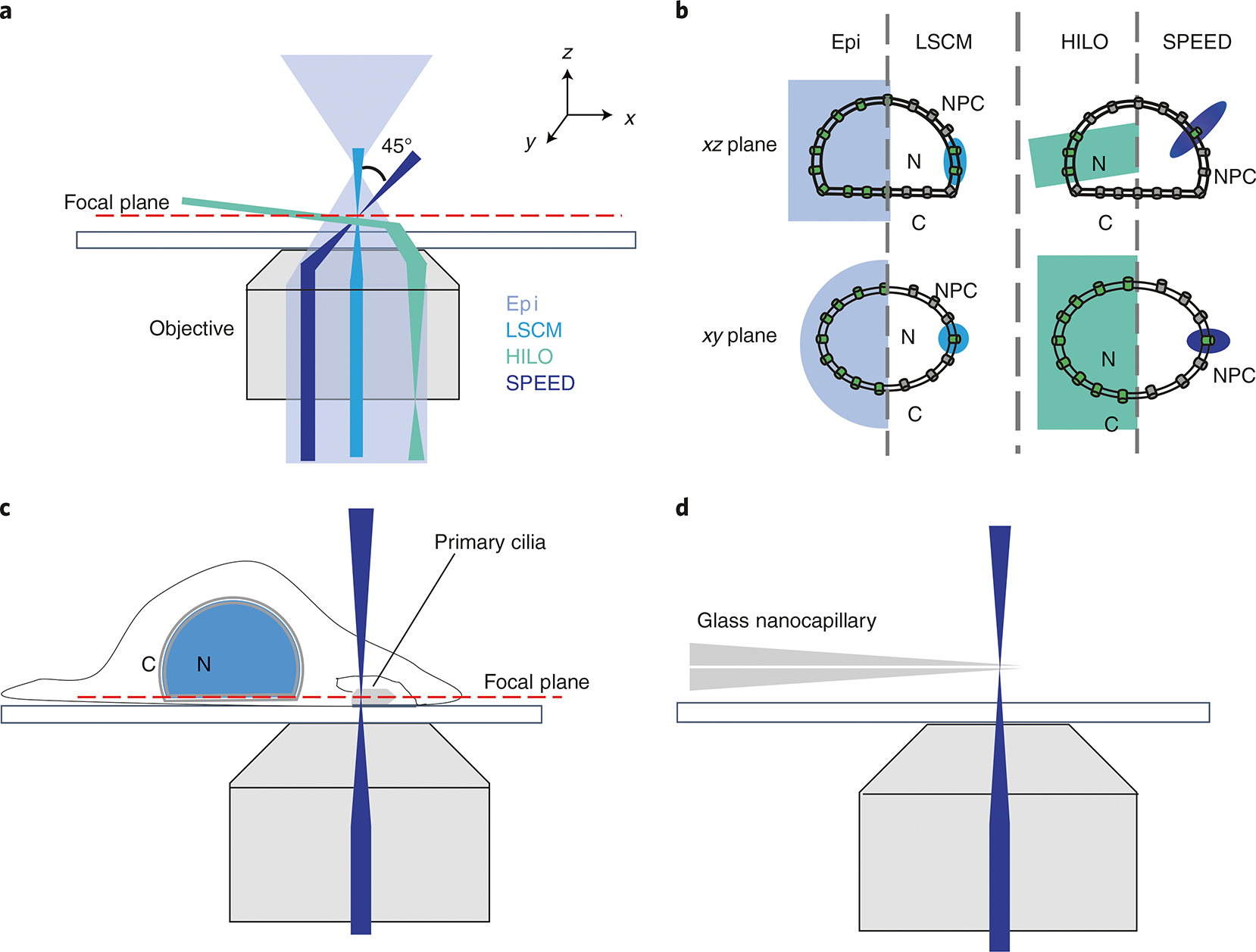
a, Schematic representation of different optical paths in different microscopes. Epi, epifluorescence microscopy. b, An example showing the different number of NPCs on the NE that could be excited by the distinct illumination patterns of these microscopes. c, A vertical illumination volume of SPEED microscopy is used to image a primary cilium. d, SPEED microscopy is used to image a GNC with the vertical illumination pattern.

However, the inclined single-point illumination volume of SPEED microscopy has better axial resolution and acceptable lateral resolution (~320–230 nm in the x, y and z directions when using a tilted laser with an angle between 35° and 55° for a 488-nm excitation laser), which allows it to excite only a single NPC in all three dimensions^33,34 (Figs. 1a and 6b).

To achieve the inclined single-point illumination volume, a standard vertical single-point illumination (as in LSCM) is established first. This is done by aligning the laser beam to pass through the central axis of the objective by adjusting the reflection mirror (Fig. 1a). Next, the center excitation beam is shifted a specific distance off the central axis of the objective using a micrometer stage, so as to generate an inclined illumination volume (Fig. 1a). The required shift distance is dependent on several parameters: the focal length of objective, the refractive indexes of the different mediums on the optical path and the inclined angle required. As shown in Fig. 1, the relationship between the inclined angle (θ₃) and the shift distance (d) follows the equation: $d=a*\tan \left[{\sin }^{-1}\left(\frac{n_{cell}}{n_{oil}}\sin {\theta }_3\right)\right]$, where the focal length of objective a = 300 μm, the refractive index in cell n_cell = 1.33 and the refractive index of immersion oil n_oil = 1.516. For example, to obtain θ₃ = 45°, d needs to be 237 μm.

Notably, SPEED microscopy shares similarities with highly inclined thin illumination (HILO) microscopy, as they are both improving axial resolution via inclined illumination⁵⁶. The key difference is that the incident beam of our SPEED microscope is focused on a spot at the focal plane, whereas the incident beam of HILO microscopy is laminated and parallel as a thin optical sheet at the target plane (Fig. 6a). As a result, HILO microscopy would simultaneously illuminate multiple NPCs on the nuclear envelope, both in the lateral and axial dimension of the illumination volume. In contrast, only a single NPC is imaged in the excitation volume of SPEED microscopy (Fig. 6b).

The inclined illumination volume is not always required when applying SPEED microscopy to image sub-diffraction-limit scale structures. For example, the vertical single-point illumination volume can be used to image sub-diffraction-limit structures that are sufficiently spatially separated. We used vertical single-point illumination to image the primary cilium⁴². This is possible because cells contain only a single primary cilium, and there is therefore no risk that multiple primary cilia are imaged simultaneously (Fig. 6c). Similarly, spatially separated GNCs could be imaged by vertical single-point illumination without simultaneous excitation of multiple GNCs⁴² (Fig. 6d). Because SPEED microscopy is a single-molecule localization microscopy approach, generating a sufficiently low density of fluorescence molecules is critical for accurate imaging in the structures of interest. For in vitro studies (for example, using GNCs⁴²) or studies using permeabilized cells (for example, by using fluorescently labeled importin-β1³⁸), we can guarantee a sufficiently low density of fluorescent molecules by controlling their concentration. It is more challenging to generate a sufficiently low concentration of proteins of interest in living cells. To ensure low levels of fluorescent molecules, we photobleach the region of interest to a completely dark state before single-molecule imaging by using a relatively higher laser power. Non-bleached fluorescent molecules from outside of the photobleached area diffuse into the region of interest, allowing us to perform single-molecule imaging.

To achieve high spatiotemporal resolution, we use a high-speed camera and generate a high laser power density at the focal plane of the objective. In our setup, we use an on-chip multiplication gain CCD camera (Cascade 128+) to capture images at a high frequency. This camera has extraordinary sensitivity for low-light-level fluorescent signals and a very high readout speed of more than 500 full frames per second (2 ms per frame) of the 128 × 128-pixel chip and up to 2,500 partial frames per second (0.4 ms per frame at 128 × 20-pixel chip). To ensure sufficient temporal resolution to track molecules of interest moving through the structure of interest, the readout speed should be set to maximally 20% of the event time of interest. For example, because the nuclear export time of a single mRNA has been reported to be ~11 ms⁴⁵, we set the readout speed at 2 ms per frame. Similarly, the readout speed is set to 0.4 ms per frame when capturing the nuclear transport of importin-β1, whose transport time is ~5–7 ms^38,39. An additional advantage of using a high detection speed is the significantly improved single-molecule localization precision for fast-moving molecules, although it should be noted that the short detection time limits the number of photons collected from the targeted molecules. To solve this problem, we recommend increasing the laser power density at the focal plane of the objective when exciting the maximum quantity of photons within such a short detection time. For example, we use an average laser power density of ~500 kW/cm² at the focal plane when imaging Alexa Fluor 647-labeled importin-β1. This is sufficient to excite more than 1,100 photons from a single four-Alexa Fluor 647-labeled importin-β1 with 400-μs detection time, which provides a lateral localization precision of ~9–11 nm³⁸.

2D data analysis

The first step in 2D image analysis is to fit each image with a 2D Gaussian fitting function to obtain single-molecule localization. In our studies, we have employed both the computer program Glimpse (https://github.com/gelles-brandeis/Glimpse) and the ImageJ plugin GDSC-SMLM (http://www.sussex.ac.uk/gdsc/intranet/microscopy/UserSupport/AnalysisProtocol/imagej/gdsc_plugins/) to fit single-molecule images and obtain information on the spatial location of single molecules, the integral fluorescence intensity of single molecules, the background intensity and the Gaussian width of single-molecule spots. The single-molecule data are then filtered based on the information obtained from single-molecule fitting. Specifically, images containing a Gaussian width of single molecules that is too low or too high are excluded as they are likely not derived from a single-molecule signal and are probably either background noise or from multiple molecules that are excited simultaneously. The SNR is calculated by using the signal intensity from the integral fluorescence intensity of single molecules and the background intensity. Typically, we select only single molecules with an SNR >10, which enables us to exclude single-molecule images that might provide inaccurate localization precision.

The localization precision for single fluorescent molecules is determined by how precisely the centroid of each detected fluorescent diffraction-limited spot was defined. For immobilized molecules, the fluorescent spot is fitted to a 2D Gaussian function, and the localization precision is determined by the standard deviation of multiple measurements of the central point. For moving molecules, the influence of particle motion during image acquisition should be considered when determining the localization precision. More specifically, the localization precision for moving substrates (σ) is determined using the following equation:

$$\sigma =\sqrt{F\left[\frac{16\left(s^2+a^2/12\right)}{9N}+\frac{8\pi b^2{\left(s^2+a^2/12\right)}^2}{a^2{N}^2}\right]}$$

where F is equal to 2, N is the number of collected photons, a is the effective pixel size of the detector, b is the standard deviation of the background in photons per pixel and $s=\sqrt{s_0^2+\frac{1}{3}D\mathrm{\Delta }t}$, wherein s₀ is the standard deviation of the PSF in the focal plane, D is the diffusion coefficient of the substrate and Δt is the image acquisition time.

In our experiments, we typically use >1,000–2,000 photons and in-focus Gaussian widths (0.5–1.0 pixel, corresponding to single GFP molecules located in the focal plane) for accurate localization of fluorescent molecules. Using the above equation, the localization precision is determined to be ≤10–20 nm with the following experimentally defined parameters: N >1,000–2,000, a = 240 nm, b ≈ 2, s₀ = 150 ± 50 nm, Δt = 0.4–2 ms and D is in the range of 0.1–3 μm² s⁻¹ for the various tested substrates.

After analysis of the 2D single-molecule trajectories, two major types of information are extracted: dynamics information and structural information. When studying transport through NPCs, the dynamics information includes the diffusion coefficient, the nuclear transport efficiency, the dwelling time and the frequency of molecules entering the NPCs⁴⁹. The structural information includes the location distribution pattern of the molecules of interest obtained by superposition of hundreds of 2D single-molecule trajectories or 2D single-molecule spatial locations^57,58. Notably, the temporal resolution for extracting the dynamics is determined by the detection speed of the CCD camera we used, which we recommend to be within 0.4–2 ms. In contrast, the temporal resolution to obtain the structural information is ~1–3 s, allowing for hundreds of single-molecule trajectories to be collected to obtain sufficient 2D single-molecule locations for 2D-to-3D transformation (see the following section).

2D-to-3D transformation

As shown in Fig. 2, the 2D spatial locations obtained for any radially symmetric structure are a projection of real 3D spatial locations in the x,y plane, which could be regarded as convolution. Therefore, the main principle behind the 2D-to-3D transformation is that 3D spatial information is recovered from 2D spatial information via deconvolution. For a radially symmetric structure such as NPCs, an area matrix in the radial dimension is generated in the y,z plane (Supplementary Fig. 1). This area matrix is used to reflect the contribution of the density of each ring to the location distribution along the y and z dimensions. Eventually, the densities in the radial dimension, or each ring, are obtained by solving the matrix equations, as detailed in the mathematical calculation shown in Supplementary Fig. 1.

SPEED microscopy and 2D-to-3D algorithm validation

When using any analytical technique, it is important to identify the measure of error in the system to characterize the accuracy of the final result. For SPEED microscopy and its 2D-to-3D algorithm, such a measure cannot be calculated in a straightforward manner due to the high degree of nonlinearity and the fact that the final 3D histograms depend on many experimental factors. Two of the most important factors that affect the final result are the single-molecule localization precision and the number of single-molecule localizations collected during imaging. For example, a poor localization precision will result in a 3D histogram that is too blurred together to obtain any detailed information, whereas a low number of single-molecule localizations often generates under-sampling artifacts in the 3D histogram. Owing to the dependence of the measurement error on these factors and in the interest of time efficiency, it is critical to evaluate the error at several points throughout the imaging and 2D-to-3D transformation experimental process. First, one should estimate the error at the outset of any experiment to ensure that the experimental limitations (for example, the reasonable estimated single-molecule localization error and the number of expected single-molecule localizations) do not prevent any biologically relevant details from being obtained. In addition, the error should be assessed once experimental data collection and analysis have been performed to ensure that the error in the system has been managed well and the results support the final biological claims.

We use Monte Carlo simulation to mathematically model the error of the system and, thereby, determine the reproducibility of obtaining accurate 3D histograms. This simulation method is chosen owing to its ease of implementation and ability to intuitively account for relevant experimental parameters—namely, the single-molecule localization precision and the number of single-molecule localizations collected. The single-molecule localization precision depends on the number of photons that can realistically be collected from a fluorophore attached to the molecule of interest and the uniformity of the background noise. The number of single-molecule localizations collected is a function of the frequency at which molecules of interest enter the area of illumination and the time frame within which single-molecule data were collected.

To model the collection of single-molecule locations in rotationally symmetric biological structures, Monte Carlo simulations are initially performed by varying the numbers of single-molecule localizations simulated along the circumference of a ring with radius R_I. Second, the single-molecule localization error (σ_LE) is added to each simulated point by sampling a value from a normal distribution with a standard deviation of σ_LE, which equals the single-molecule localization error measured in our experiments. Third, the 2D-to-3D transformation algorithm is performed on the y-dimensional portion of the simulated data. This is done to simulate the loss of z-dimensional information that occurs during the imaging process. The peak position of the 3D histogram (R_M), which might deviate from R_I due to limitations of simulated localization error and the number of localizations, is then obtained via Gaussian fitting as it would be in normal experimental results (Fig. 7a). This process is then performed 10,000 times to obtain 10,000 R_M values whose population mean converged on R_I. Lastly, we determine what percentage (reproducibility rate) of R_M values fall within R_I ± σ_LE, because this determines what is the chance of any given experiment falling within this acceptable range (Fig. 7b). We define this range as such because any single R_M value can only be theoretically localized within a range of approximately two standard deviations centered on its Gaussian fitting. Overall, minimizing the single-molecule localization error and maximizing the number of single-molecule localizations will yield the best reproducibility rate.

Fig. 7 |. Validation of the reproducibility of SPEED microscopy and its 2D-to-3D histogram.

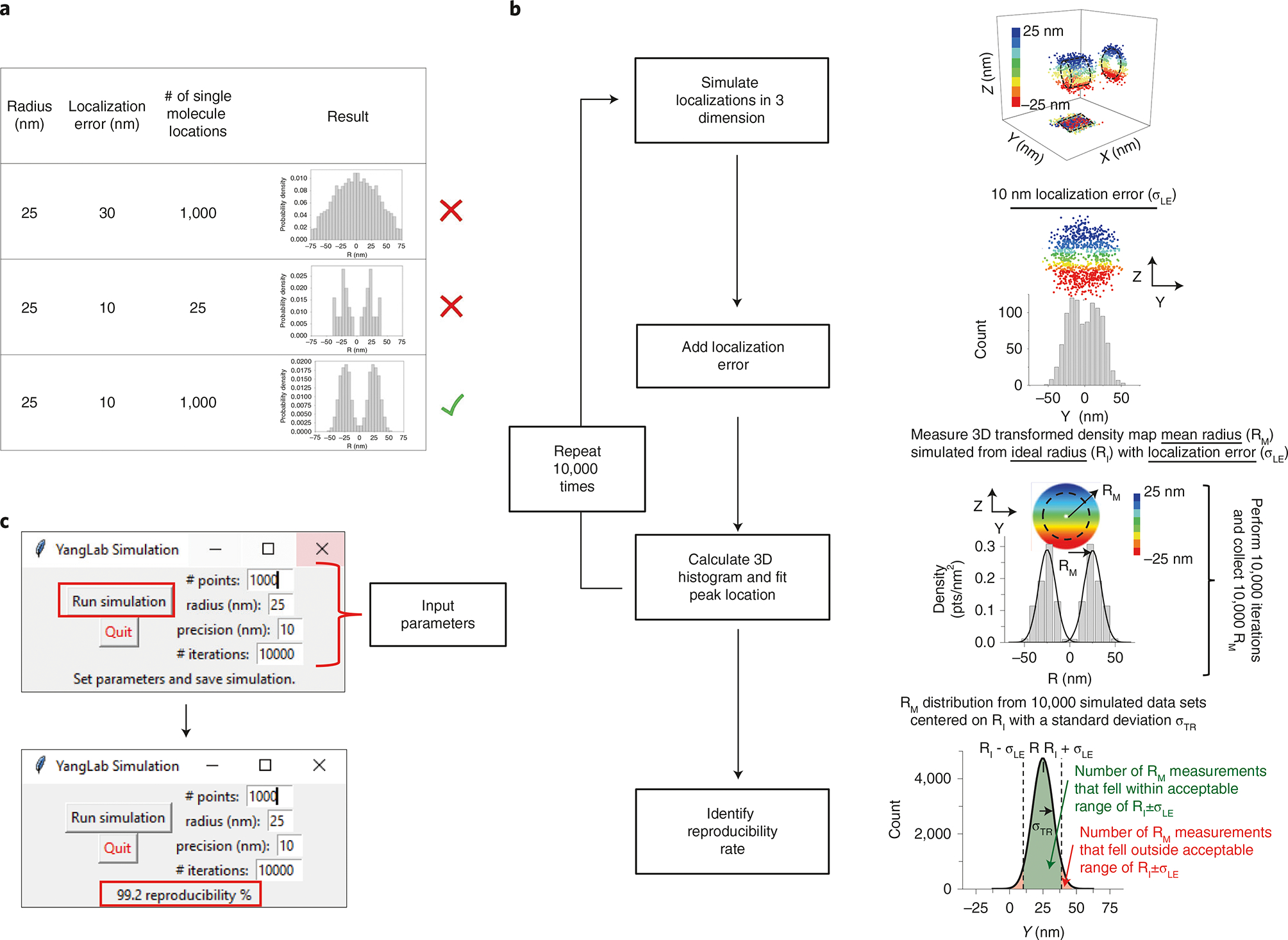
a, Table showing the effect of poor single-molecule localization precision and a low numbers of single-molecule localizations. b, Flowchart outlining the simulation process for determining the reproducibility rate. c, Graphical user interface for the reproducibility rate simulation. Results are displayed in the message section after the simulation has been run.

As mentioned above, it is important to assess the reproducibility rate after experiments and data analysis have been performed. To simplify determination of the reproducibility rate, we provide Python scripts at https://github.com/YangLab-Temple/Master that can run on any computer with a Python installation. Running this script launches a graphical user interface where experimental parameters can easily be inputted and the simulation run (Fig. 7c).

Materials

Biological materials

• Cell line with a fluorophore tagged to a structural element of the rotationally symmetric structure of interest. In the examples shown in this protocol, the NPC was analyzed using HeLa cells stably expressing mCherry fused to the N-terminus of the NPC structural protein POM121 (HeLa POM121-mCherry (RRID: CVCL_A916)). To interrogate the primary cilium, we use NIH-3T3 cells stably expressing intraflagellar transport protein homolog 20 (IFT20) tagged at the C-terminus with enhanced GFP (eGHP) (NIH 3T3 IFT20-GFP (RRID: CVCL_A9G7)). This cell line was chosen because serum starvation results in cell cycle arrest and ciliogenesis for most of these cells⁵⁹ ! CAUTION The cell lines used in your research should be regularly checked to ensure that they are authentic and not infected with mycoplasma.

Reagents

• Purified protein of interest labeled with a fluorescent dye (see ‘Reagent setup’). Consult the ‘Experimental design’ section to determine whether purified proteins or a plasmid containing the protein or mRNA of interest should be used

• A plasmid containing an open reading frame (ORF) that expresses the protein of interest fused to a fluorescent protein (see ‘Reagent setup’). Consult the ‘Experimental design’ section to determine whether purified proteins or a plasmid containing the protein or mRNA of interest should be used

• A plasmid containing an ORF for the MCP dimer fused to a fluorescent protein and a plasmid that encodes the mRNA sequence of interest fused to 24 MS2 stem loops (see ‘Reagent setup’). Consult ‘Experimental design’ to determine whether purified proteins or a plasmid containing the protein or mRNA of interest should be used

• HEPES (Thermo Fisher Scientific, cat. no. BP310–500)

• KOAc (Thermo Fisher Scientific, cat. no. P178–3)

• NaOAc (Thermo Fisher Scientific, cat. no. AA4168522)

• MgOAc (Thermo Fisher Scientific, cat. no. PR-L4581)

• EGTA (Thermo Fisher Scientific, cat. no. 32–462-625GM)

• Digitonin (Sigma-Aldrich, cat. no. D141–100MG)

• Polyvinylpyrrolidone (PVP, 360 kDa; Thermo Fisher Scientific, cat. no. AAJ6138130)

• Dulbecco’s Modified Eagle Medium (DMEM), high-glucose GlutaMAX (Gibco/Thermo Fisher Scientific, cat. no. 10566016)

• FBS (Thermo Fisher Scientific, cat. no. 10–439-024)

• Streptomycin (Thermo Fisher Scientific, cat. no. ICN10055625)

• Penicillin (Thermo Fisher Scientific, cat. no. ICN19453780)

• Opti-MEMTM Reduced Serum Medium (Gibco/Thermo Fisher Scientific, cat. no. 31985088)

• Trypsin-EDTA (0.25% (wt/vol)), phenol red (Gibco/Thermo Fisher Scientific, cat. no. 25200056)

• TransIT-X2 Transfection Reagent (Mirus, cat. no. MIR 6000)

• Ni:NTA Superflow (25 ml) (Qiagen, cat. no. 30410)

• Alexa Fluor 488 C₅ Maleimide (Invitrogen/Thermo Fisher Scientific, cat. no. A10254)

• Digitonin (Sigma-Aldrich, cat. no. D141–100MG) ! CAUTION Toxic if swallowed, inhaled or comes into direct contact with skin. Care should be taken to wear gloves and safety goggles when handling this reagent.

• Gibco 1× PBS, pH 7.4 (mnb Gibco/Thermo Fisher Scientific, cat. no. 10010023)

Equipment

Cell culture

• Glass-bottom culture dishes, 35-mm Petri dish, 14-mm microwell with no. 0 cover glass (0.085–0.13 mm) (MatTek, cat. no. P35G-0–14-C)

• Corning 25 cm² vented cell culture flasks (Sigma-Aldrich, cat. no. CLS430639)

Microscope

• Olympus IX81 equipped with a 1.4-NA ×100 oil-immersion apochromatic objective (UPLSAPO 100XO, Olympus) or any suitable inverted fluorescence microscope

• Low autofluorescence immersion oil (Olympus, cat. no. IMMOIL-F30CC)

Camera

• On-chip multiplication gain CCD camera (Cascade 128+; Roper Scientific)

Lasers

• Obis solid-state 561-nm LS 50-mW laser (Laser Head 1230935, Laser System 1230936, Coherent)

• Obis solid-state 488-nm LX 50-mW laser (Laser Head 1185053, Laser System 1178764, Coherent)

Filter sets and mirrors

• Dichroic filter (Di01- R405/488/561/635-25×36, Semrock)

• Emission filter (NF01- 405/488/561/635-25×5.0, Semrock)

• Two circular variable metallic neutral density (ND) filters (Newport, cat. nos. 50G02AV.1 and 50Q04AV.2)

• Micrometer stage consisting of one beam steering accessory, top, SM Micrometers (Newport, cat. no. 670-RCT-M) and one beam steering accessory, bottom (Newport, cat. no. 670-RCB) mounted on one damped optical post, gear rack mounting base, 14 in. height, 1.5 in. diameter (Newport, model 75)

Table

• A microscope on a pneumatic isolator that is pre-mounted to a research-grade optical table (Newport, cat. no. RS4000-46-12)

Software

• Slidebook software package (https://www.intelligent-imaging.com/slidebook, Intelligent Imaging Innovation)

• FIJI ImageJ⁶⁰ for image analysis (https://imagej.net/Fiji/Downloads)

• GDSC SMLM ImageJ plugin (http://www.sussex.ac.uk/gdsc/intranet/microscopy/UserSupport/AnalysisProtocol/imagej/gdsc_plugins/)

• 2D-to-3D simulation script ‘simulation_gui.py’ (https://github.com/YangLab-Temple/Master/tree/master/JPC%20simulations%202019/Figure%208%20-%20labeling%20efficiency)

• OriginPro 2019 (https://www.originlab.com/2019, OriginLab)

• MATLAB (https://www.mathworks.com/products/matlab.html, MathWorks)

• 2D-to-3D transformation script ‘2D_to_3D.m’ (https://github.com/YangLab-Temple/Master)

• Python 3 (https://www.python.org/downloads/) and Python libraries tkinter, csv, random, os, sys, numpy, scipy and math

Reagent setup

Transport buffer

Combine 20 mM HEPES, 110 mM KOAc, 5 mM NaOAc, 2 mM MgOAc and 1 mM EGTA and adjust to pH 7.3. This buffer can be stored at room temperature (~21 °C) for up to 1 year.

Permeabilized buffer

Supplement transport buffer with 40 μg/ml of digitonin. This buffer is always prepared freshly before experiments.

PVP buffer

Supplement transport buffer with 1.5% (vol/vol) PVP (360 kDa). This buffer is always prepared freshly before experiments.

Cell culture media

Supplement DMEM with high-glucose GlutaMAX, 10% (vol/vol) FBS, 10 mg/ml of streptomycin and 100 U/ml of penicillin. This buffer can be stored at 4° for 30 d without re-filtering as long as there are no signs of contamination. ▲CRITICAL The culture media might need to be changed if other cell lines are used.

Protein of interest labeled with an organic dye

For various proteins of interest, different purification and labeling approaches can be used. In our research, for example, His-tagged human importin-β1 protein was expressed in BL21 strain of Escherichia coli and purified by Ni-NTA Superflow (Qiagen), MonoQ and Superdex 200 (Amersham) chromatography³⁸. Then, solvent-accessible cysteines on the importin-β1 were labeled with Alexa Fluor Maleimide dye (Invitrogen) for 2 h to obtain a density of four fluorescent dyes per protein molecule.

Plasmid encoding the protein of interest

Generate a plasmid bearing an ORF that expresses the protein of interest as well as an FP. In this protocol, we use a plasmid obtained from Geneservice, which encodes the nuclear envelope transmembrane protein NET49 (IMAGE 3959506). This plasmid was polymerase chain reaction amplified from its IMAGE clone, and the digestion sites NheI and BamHI were added to facilitate C-terminus tagging with eGFP⁴⁶ (Fig. 4f,l). All plasmids are available from the corresponding author upon reasonable request.

Plasmid encoding the mRNA of interest

The system used for imaging single-molecule mRNA is a bipartite system that requires a plasmid containing an ORF for the MCP dimer fused to an FP and a plasmid that encodes the mRNA sequence of interest fused to 24 MS2 stem loops. This MS2 loop system was originally a generous gift from Robert Singer (Albert Einstein College of Medicine). We modified the system from its original form⁶¹ by switching the YFP to mCherry and attaching the 24 MS2 stem loop sequence to the 3′ end of the Photinus pyralis luciferase gene (Fig. 3). All plasmids are available from the corresponding author upon reasonable request.

Procedure

Cell preparation ● Timing 6–7 d

▲CRITICAL All procedures in Steps 1–4 should be performed under sterile conditions on a flow cabinet.

• 1Resuscitate required cells at least 1 week before transfection. Thaw frozen stocks (−80 °C) of cells to 37 °C and then put into a 25-cm² culture flask with 4–5 ml of pre-warmed (37 °C) cell culture media (see ‘Reagent setup’).

  ▲CRITICAL STEP In the example demonstrated in this protocol, the cell line is a stable expressing POM121-GFP or POM121-mCherry HeLa cell line. The culture media and cell culture conditions might need to be changed if other cell lines are used.

• 2Place the culture flask into an incubator at 37 °C with 5% CO₂ overnight. Exchange the culture media with fresh supplemented DMEM the next day and put back in the incubator at 37 °C with 5% CO₂ for an additional 1 d.
• 3Split the culture cells at least three times over the course of 1 week to guarantee that cells will be at optimal health for transfection and for the SPEED microscopy imaging experiment.

  ▲CRITICAL STEP Optimal conditions for imaging the HeLa cell lines described here are when cells are grown at ~90–95% confluency with ≤5% of the culture being apoptotic.

• 4
  Introduce the fluorescently labeled molecules of interest into cells. Follow Option A for the transfection of a plasmid expressing FP-labeled proteins into live cells. Follow Option B for adding proteins labeled with an organic dye into permeabilized cells.

  1. Transfecting live cells

     1. Two days before SPEED microscopy experiments, split the cells and plate ~1 × 10⁶ cells in 1 ml of cell culture media per dish onto 2–4 glass-bottom optical dishes. Place the dishes back into the incubator at 37 °C with 5 % CO₂ overnight.
        ▲CRITICAL STEP The cells plated onto the glass-bottom dishes should be ~50% confluent on the next day to achieve optimal transfection results.
     2. Prepare a transfection mixture with the plasmid encoding the FP-tagged protein of interest. For each dish, we combine 0.5–1 μg of plasmid and 3 μl of transfection reagent (TransIT X2 (Mirus)) in ~95 μl of Opti-MEM reduced-serum medium by gently flicking.
        ▲CRITICAL STEP If the transfection reagent is stored in the fridge, it must be warmed to room temperature before preparing mixture.
        ▲CRITICAL STEP Untreated and empty vector transfection control plates can be set up as well to assess the effect of experimental transfection on cell health and viability.
     3. Allow the transfection mixtures to incubate at room temperature for ~15–20 min.
     4. Add transfection mixtures dropwise to the glass-bottom optical dishes from Step 1 and allow the cells to incubate at room temperature for 2–3 min.
     5. Place the dishes back in the incubator at 37 °C with 5% CO₂ overnight so that FP-tagged protein will have reasonable expression levels for the SPEED microscopy experiments.
     6. On the day of the SPEED microscopy imaging experiment, remove the culture media from the dishes. Wash the cells twice with 1 ml of pre-warmed (37 °C) PBS.
        ▲CRITICAL STEP The cell culture media should be removed to reduce fluorescent background signal as a result of the phenol red that is included in the DMEM.
     7. Remove the PBS, add 1 ml of pre-warmed (37 °C) transport buffer to each dish and incubate the transfected cells at room temperature for 30–45 min.
        ▲CRITICAL STEP Transport buffer incubation is used to reduce the movement of the nuclear envelope during SPEED microscopy.
  2. Adding proteins labeled with an organic dye into permeabilized cells

     1. One day before the SPEED microscopy experiments, split the cells and plate ~1 × 10⁶ cells in 1 ml of cell culture media per dish onto 2–4 glass-bottom optical dishes. Place the dishes back into the incubator at 37 °C with 5% CO₂ overnight.
        ▲CRITICAL STEP The cells plated onto the glass-bottom dishes should be ~50% confluent on the next day to achieve optimal transfection results.
     2. Remove culture media from the dishes and wash the dishes twice with 1 ml of pre-warmed (37 °C) PBS.
     3. Remove the PBS and incubate the cells with 1 ml of pre-warmed (37 °C) transport buffer at room temperature for 30–45 min.
        ▲CRITICAL STEP Transport buffer incubation is used to reduce the movement of the nuclear envelope during SPEED microscopy.
     4. Replace the buffer with 1 ml of transport buffer containing 40 μg/ml of digitonin and incubate for 2–3 min at room temperature. Remove the buffer and wash the cells at least three times with 1 ml of PVP buffer to thoroughly remove the digitonin.
        ▲CRITICAL STEP Make sure not to exceed the 2–3-min incubation time. Long exposure of cells to digitonin could cause osmotic swelling of the nuclei before imaging.
     5. Remove the PVP buffer. Add 1 ml of PVP buffer containing the protein of interest labeled with an organic dye in the appropriate concentration. In our case, the concentration of Alexa Fluor-labeled importin-β1 is 1 nM. For other organic dye-labeled proteins, the optimal concentration might be different. Immediately proceed to Step 5 to start with SPEED microscopy imaging.
        ▲CRITICAL STEP Unlabeled protein may be added to the cells in place of labeled protein for a control of the baseline level of fluorescence.

SPEED microscopy ● Timing 4–5 h

▲CRITICAL A working and properly aligned epifluorescence microscope is a prerequisite for successful SPEED microscopy.

• 5To ensure that a parallel laser beam reaches the back aperture of the objective, remove the expansion and alignment optics that guide the excitation light coming from the back port.
• 6Align the required lasers to precisely overlap their light paths as they reach to the microscope objective. For example, as shown in Fig. 1, a 488-nm laser and a 561-nm laser are used to excite an NPC labeled with POM121-GFP and mCherry-labeled soluble protein. To precisely overlap the two laser paths, direct both laser paths through the center of two irises by adjusting pairs of mirrors and dichroic filters (Fig. 1a).
• 7Adjust the reflection mirror mounted on the micrometer stage to direct the laser beams through the central axis of the objective to achieve vertical excitation illumination.
• 8For an inclined illumination, shift the laser beams off the central axis of the objective by horizontally moving the micrometer stage, as shown in Fig. 1b. The cross-sectional diameter of the focal spot size in the x,y plane of our setup is ~210 nm (the vertical illumination) and ~240 nm (with inclined illumination at an angle of 45°) when using a 488-nm laser for illumination and a 1.4 NA objective. The typical laser power that reaches the focal point is 0.2 mW (2 × 10⁻⁷ kW). With a focal spot size of ~3.5 × 10⁻¹⁰ cm² (vertical) or 4.5 × 10⁻¹⁰ cm² (inclined), the average optical density at the focal point is ~450–570 kW/cm².

  ? TROUBLESHOOTING

• 9Place the glass-bottom optical dishes containing the prepared cells from Step 4 on the stage of the SPEED microscope. Use a ×100 oil immersion objective to visualize the cells under bright field (white transmission light) and bring the subcellular structure of cells into the focal plane by adjusting the focal adjustment knob. For example, we bring the equator of the nuclear envelope into the focal plane when imaging nuclear transport through the NPC.

  ▲CRITICAL STEP Target cells with a healthy morphology under bright field. Only cells in interphase should be selected. Cells undergoing mitosis should be avoided owing to the fact that NPCs and the nuclear envelope might be partially disassembled, which would potentially alter routes for labeled proteins into and out of the nucleus.

• 10
  Follow Option A for imaging transfected cells as prepared in Step 4. Follow Option B for imaging permeabilized cells as prepared in Step 4.

  1. Imaging transfected cells

     1. Use a mercury lamp with the appropriate filter set to identify cells with sufficient expression of the FP-labeled protein of interest to achieve an SNR of at least 3–5.
     2. Move the center of the laser illumination volume to the biological region of interest. In this case, the left or right edge of the nuclear envelope equator (tangent to the edge of the nuclear envelope) is used.
     3. Use the ND filters in the laser’s light path to set the photobleaching laser power and excitation laser power. Generally, in our experiments, the photobleaching laser power is 1–10 mW (after passing through the ND filter), whereas the excitation laser power at the focal plane of the objective for single-molecule imaging is ~10% of the photobleaching laser power.
     4. Capture a bright-field and fluorescent image of the equator at the equator of the nuclear envelope (NE) using SlideBook. Set the exposure time to 500–1,000 ms, gain to 2 and intensification to 1,000–2,000.
        ▲CRITICAL STEP This image will be used as a comparison to determine if the NE has shifted during imaging. Also, check cell viability if any of the following would happen: distortion of cell or NE, adherent cells detach from the culturing flask, plasma membrane blebbing, large vacuoles showing up or fluorescent proteins aggregate.
        ? TROUBLESHOOTING
     5. Photobleach a small area containing the FP-labeled structure for 10–30 s. We typically use a photobleaching area of ~1 μm in diameter.
        ▲CRITICAL STEP The illumination volume needs to be photobleached to be thoroughly dark within 30 s.
        ? TROUBLESHOOTING
     6. Engage the optical chopper at 2-Hz rotation speed with an on time of 1/10 of the total frames recorded (Fig. 1c).
        ▲CRITICAL STEP The optical chopper is used to reduce photobleaching and phototoxicity during high laser power illumination.
     7. Excite the FP-labeled proteins in the illumination area and record a video for 30 s with SlideBook. By using SlideBook to record videos, these three parameters are reset on the Focal Controls window for video recording. Exposure time: 0.4 or 2 ms; gain: 3; intensification: 4,000.
        ▲CRITICAL STEP Excessively long videos might cause unacceptable shifting of the NE or NPC. Care should be taken to identify the mobility of the structure being imaged before and after experiments are done, as shown in Step 10A(iv). Ideally, movement of less than several nanometers during the imaging time window is acceptable.
        ? TROUBLESHOOTING
     8. To ensure the health and viability of the cells, replace the transport buffer in the optical dish with fresh DMEM supplemented with FBS. Incubate the optical dish overnight at 37 °C with 5% CO₂. Cells are considered to be healthy if they continue to grow and split normally after the imaging experiments.
        ▲CRITICAL STEP We typically complete measurements in a live cell within 2 min. Under our laser power setting, we do not observe photodamage after 2 min of illumination based on the tests below. First, we test photodamage or check viability via cell and NE morphology. For example, we snap the bright-field and fluorescent image of cells before and after laser illumination, as stated in Step 10A(iv). Then, check if any of the following would happen: distortion of cell or NE, adherent cells detach from the culturing flask, plasma membrane blebbing, large vacuoles showing up or fluorescent proteins aggregate. If none of these happened, finally, we keep culturing the irradiated cells overnight under the normal culture condition, and the cell is considered healthy if it grows or splits normally, as detailed in Step (viii).
  2. Imaging in permeabilized cells

     1. Use a mercury lamp with the appropriate filter set to identify cells that have incorporated levels of the fluorescently labeled protein of interest to achieve an SNR of 3–5.
     2. Move the center of the laser illumination volume to the left or right edge of the NE equator (tangent to the edge of the NE). For any given biological structure to be imaged, the optical axis should be oriented perpendicular to the long axis of the cylindrical structure.
     3. Use the ND filter in the laser light path to set the exciting laser power. Generally, in our experiments, the exciting laser power at the focal plane of the objective for single-molecule imaging is between 0.1 and 1 mW.
     4. Excite a single FP-labeled structure (e.g., a single NPC) with excitation laser.
     5. Use the Slidebook to take an image of the structure of interest: Open Slidebook > select ‘File’ > ‘New slide’ > so that a new slide is shown. Click ‘Focus window’ to open the Focal Controls window. Select ‘Camera’ and specify the following parameters:

Parameter	Setting
Camera	Cascade
Exposure	500–1,000 ms
Gain	2
Intensification	1,000–2,000
Filter set	Cascade-128

Navigate to ‘Laser’ and click ‘Snap’ to save the image in the new slide. Save the new slide to a folder.

▲CRITICAL STEP Overexposure and saturation of the image should be avoided.

1. Engage the optical chopper at a 2-Hz rotation speed with an on-time of 1/10 of the total frames recorded (Fig. 1c).

   ▲CRITICAL STEP The optical chopper is used to reduce photobleaching and phototoxicity during high laser power illumination.

2. Excite the organic dye-labeled proteins in the illumination volume with excitation laser.

   ? TROUBLESHOOTING

3. Use SlideBook to record videos of the dye-labeled protein. Modify the parameters in the Focal Controls window from Step 10B(v).

Parameter	Setting
Camera	Cascade
Exposure	0.4–2 ms
Gain	3
Intensification	4,000
Filter set	Cascade-128

Click ‘Stream’ and check the ‘Start recording when start button clicked’ box. Click ‘Start’ to start recording a video for 30–60 s. Click ‘Stop’ to stop recording, and click ‘OK’ to save the video in the folder specified in Step 10 B(v).

▲CRITICAL STEP Recording longer videos might cause unacceptable shifting of the NE or NPC. Care should be taken to identify the mobility of the structure being imaged before experiments are done. Ideally, movement of less than several nanometers during the imaging window is acceptable.

? TROUBLESHOOTING

2D data analysis ● Timing 3–6 h

• 11Convert the video file (.SPL) generated by SlideBook into an image sequence in .tiff format using SlideBook as follows. Load the movie file in SlideBook and navigate to ‘Image’ > ‘Export’ and click ‘Channel intensities as a 16-bit .tiff file’. A dialog box will then open allowing the destination folder to be designated. Uncheck ‘Write Log File’, to prevent non-.tiff format files from being located within the destination folder. Check ‘Separate File for Each Plane’ and click ‘OK’. This will write each frame of the selected video, in order, to the designated folder.
• 12Use the ImageJ2/Fiji plugin ‘GDSC-SMLM’ by selecting ‘Plugins’ > ‘GDSC SMLM’ > ‘Fitting’ > ‘Peak Fit’ or ‘Peak Fit (series)’.
• 13The ‘Select image series’ window is shown. Double click on the folder containing the image sequence. The ‘Peakfit’ or ‘PeakFit (series)’ window is now shown.
• 14Set the following peak-fitting parameters:

Parameter	Setting
Calibration (nm/px)	240
Gain	76
Exposure (ms)	0.4 or 2
Precision (nm)	≤10 or 20
Min width factor	0.5–1.5
Width factor	2
Other parameters	Default

▲CRITICAL STEP The ‘Calibration’ is the pixel size of the microscope camera. In our case, the Cascade camera has a pixel size of 240 nm/px at our given magnification. The ‘Gain’ is the ratio of the raw intensity values from the camera to photons and is dependent on the gain and intensification parameters set in SlideBook in the Focus Control window. ‘Exposure time’ is equal to exposure time set in SlideBook in the Focus Control window as well. ‘Precision’ is a minimum precision for filtering data. ‘Width factor’ uses the range of the 2D Gaussian fitted width data for filtering. Other parameters can also be changed following the manual⁶².

• 15Check the boxes for ‘log progress’, ‘binary results’ and ‘results in memory’.
• 16Select an output file directory for ‘File-output’.
• 17Click ‘OK’ and continue clicking ‘OK’ until the program runs. Once completed, the Fit Results window will be shown. The Fit Results dataset is saved automatically to the output file directory specified in Step 12.
• 18Save the Fit Results as an Excel file by navigating to ‘File’ > ‘Save as’, selecting the save directory and clicking ‘Save’.
• 19For further filtering, navigate to ‘Plugins’ > ‘GDSC SMLM’ > ‘Results’ > ‘Filter Results’, select the dataset parameters to filter and click ‘OK’. The filter results window will now display. Here, we filter the Fit Results dataset by setting several parameters: ‘Max Drift’, ‘Min Dignal’, ‘Min SNR’, ‘Min Precision’, ‘Min Width’ and ‘Max Width’. In our case, ‘Min SNR’ is set to at least ‘10’ for acquiring single-molecule data with high localization precision. The width range is set to 0.5–1.5 for excluding background noise and multiple-molecule data.

  ▲CRITICAL STEP These parameters are set based on the properties of specific fluorescent molecules and proteins of interest. The parameter set might need to be adjusted for different fluorescent molecules.

• 20Click ‘OK’. The filter result is saved automatically to the output file directory specified in Step 16.
• 21
  Follow Option A to obtain 2D location distribution information of the filtered data. Follow Option B to obtain dynamic information of the filtered data.

  1. Analysis for 2D location distribution

     1. Use the ‘File’ > ‘Save’ function in Excel to save the file.
     2. In ImageJ2/Fiji, navigate to ‘Plugins’ > ‘GDSC SMLM’ > ‘Results’ > ‘Results manager’. The peak results manager window is shown. Select the Excel sheet containing the filtered data for ‘input’ and select ‘Calibrated’ for ‘Results table’.
     3. Click ‘OK’ and continue clicking ‘OK’ until the Fit Results window is shown.
     4. Save the Fit Results as an Excel file by navigating to ‘File’ > ‘Save as’, selecting the save directory and clicking ‘Save’.
     5. Open the Excel file containing the filtered results.
     6. Obtain the coordinates of the fluorescently labeled proteins by subtracting the coordinates of the structure from the coordinates of all single-molecule localizations.
     7. Open OriginPro 2019 and then select ‘Blank Workbook’ in the New Workbook window.
     8. Copy the coordinates of the normalized localizations (from Step vi) and paste into columns A(x) and B(y) in the workbook.
     9. Plot the 2D location distribution of proteins of interest by selecting both column A(x) and B(y) > right click, navigating to ‘plot’ > ‘symbol’ and clicking ‘scatter’.
     10. Plot the frequency distribution histogram for either the x or y dimension by selecting either column > right click and clicking ‘frequency count’ to open the Frequency Counts window.
     11. In ‘computation control’, set the proper ‘minimum bin beginning’ and ‘maximum bin end’, check the box for ‘step by bin size’ and set proper ‘bin size’. The ‘minimum bin beginning’ should be 0, and the ‘maximum bin end’ should be the maximum value in the data set. The ‘bin size’ should be set small enough to visualize the data features but large enough to avoid noise. Typically, 5–10 nm is acceptable.
     12. Click ‘OK’. The frequency count result is shown in a new sheet. Select the column ‘Bin Center’ (or ‘Bin End’) as well as the column ‘Count’ > right click, navigate to ‘plot’> ‘Column/Bar/Pie’ and click ‘Column’.
  2. Analysis for dynamic information

     1. To find the traces or trajectories of single molecules in ImageJ2/Fiji, navigate to ‘Plugins’ > ‘GDSC SMLM’ > ‘Calibration’ and click ‘Trace Diffusion’.
     2. To filter the single-molecule raw data, set ‘Distance Threshold’, ‘Distance Exclusion’ and ‘Min Trace Length’ before navigating to uncheck the box for ‘Ignore ends’ and check ‘Save traces’. Finally, click ‘OK’.
        ▲CRITICAL STEP ‘Distance Threshold’ is the longest distance between two consecutive locations in the same trace. ‘Distance Exclusion’ is the shortest distance between two consecutive locations in the same trace. ‘Min Trace Length’ is the minimum number of locations in one trace. In our case, set ‘Distance Threshold (nm)’ to 200 and ‘Distance Exclusion (nm)’ to 0.
     3. The Trace File window is now displayed. Select the save directory and click ‘OK’. The ‘Trace Diffusion Data Summary’ window is shown, and the trace results are saved as an Excel file in the specified directory.
     4. The ‘Trace Diffusion Data Summary’ window provides the diffusion coefficient of the fluorescent molecule of interest, which is important dynamic information and can be saved in a separate file for future use.
     5. Open the trace results that were saved as an Excel file in Step (iii).
     6. Obtain the normalized coordinates of traces by subtracting the coordinates of the structure of interest (e.g., the NPC) from the coordinates of all traces of the molecules of interest.
     7. Open the OriginPro 2019 and then select ‘Blank Workbook’ in the New Workbook window.
     8. Copy the coordinates of each normalized trace from Step (xiv) and paste this information into columns A(x) and B(y) in the workbook.
     9. Plot the 2D trajectory of molecules of interest by selecting both column A(x) and B(y) > right click, navigating to ‘plot’ > ‘Line+symbol’ and clicking ‘Line+symbol’.
     10. (Optional) Based on the 2D trajectory of interest molecules, determine the nuclear transport time of the molecules of interest. In addition, use the obtained information to judge whether the molecules pass successfully through the NPC and calculate the nuclear transport efficiency.
         ▲CRITICAL STEP The transport time is defined as the time required by molecules to diffuse through the NPC. The transport efficiency is the percentage of successful transport trajectories (events) of all transport trajectories. We recommend calculating the nuclear transport efficiency and transport time based on hundreds of nuclear transport trajectories (events) collected from more than ten different cells.
     11. (Optional) Count the number of trajectories of molecules of interest entering a single NPC within an ~30–60-s timeframe. Divide the number of trajectories by the total time elapsed on the video clip to obtain the entrance frequency of the molecule of interest into the NPC.
         ▲CRITICAL STEP For statistically accurate calculation of the entrance frequency, we recommend to collect data from more than ten NPCs per cell from ten different cells.

(Optional) 2D-to-3D transformation ● Timing 1–5 h

▲CRITICAL STEP This section should be used when one desires to obtain the 3D radial density histogram from the 2D single-molecule distribution.

• 22Open the Excel file from Step 21 Option (A) and copy the normalized 2D coordinates of the molecules of interest.
• 23Paste these 2D coordinates into a new Excel file, with the x coordinates in column ‘A’ and the y coordinates in column ‘B.’ Save the file in a .csv format.

  ▲CRITICAL STEP Only numbers are allowed in the .csv file. Do not put letters, symbols or formulae in .csv format.

• 24Use MATLAB to open the 2D-to-3D transformation code ‘2D_to_3D.m’.
• 25Set the working directory to the folder containing the .csv file from Step 23 and set the target file to the file name of the .csv file from Step 23. Set the axial region ranges (x dimension; Fig. 2a) required to conduct 2D-to-3D transformation and set the bin size (i) along the radial dimension (r dimension; Fig. 2a). Generally, the bin size (i) is set to the half of single-molecule localization precision (as determined in the peak fitting results from ‘GDSC-SMLM’). Set the length of the axial region range to the single-molecule localization precision.
• 26Run ‘2D_to_3D.m’. The results are saved automatically as a .csv file in the working directory specified in Step 23. In the results file (.csv), a third column is created that specifies the density of the molecules of interest along the radial dimension of the selected axial region.
• 27Repeat Steps 22–26 to conduct 2D-to-3D transformation for the remaining axial region ranges until the entire axial region of the structure of interest has been transformed.
• 28Collect the densities of the molecules of interest along the radial dimension (from the third column in the results files created in Step 26) from all axial regions and combine these data together in a new Excel file.
• 29To normalize intensity data from all axial regions, divide each intensity by the maximum value of these data. This results in the density probabilities along radial dimensions in all axial regions of the structure of interest (Fig. 8a).
• 30Multiply all density probabilities by 255 to convert the density probabilities to the intensity values of a grayscale map (Fig. 8b).
• 31To make a radial-view density probability map for an axial region (Supplementary Fig. 1) using ImageJ2/Fiji, the following steps should be followed. First, import a ‘radial rings’ image to the ImageJ2/Fiji (Supplementary Fig. 1). Then, double click ‘Color picker’ and ‘Foreground color’.

  Next, navigate to set ‘Red’, ‘Green’ and ‘Blue’ to an intensity value obtained at a certain radius from Step 30. Finally, click ‘OK’ and ‘Flood Fill Tool’ to fill the ring at corresponding radiii in the ‘radial rings’ image (Fig. 8c).

• 32Repeat Step 31 until the ring image is filled at all analyzed radii in ‘radial rings’.
• 33Navigate to ‘Process’ > ‘Filters’ > ‘Gaussian Blur’ and click ‘Gaussian Blur’. In the window that is shown, set ‘Sigma (Radius)’ to ‘4’ and click ‘OK’. To obtain a radial-view density probability map for an axial region, select ‘File’ and ‘Save’ (Fig. 8d).
• 34Repeat Steps 31–33 until a radial-view density probability map for all axial regions has been generated.
• 35Navigate to ‘File’ > ‘Open’ and open the all radial-view density probability maps in sequence of the axial region.
• 36Select the first open radial-view density probability map and navigate to ‘Image’ > ‘Duplicate’ to duplicate the selected map. Duplicate the selected map N times. $N=\frac{\text{length}\text{of}\text{axial}\text{region}}{10\text{nm}}-1$
• 37Repeat Step 36 in sequence for all other radial-view density probability maps.
• 38Navigate to ‘Image’ > ‘Stacks’ > ‘Images to Stack’ to open the Images to Stack window. Click ‘OK’ to generate the stack.
• 39Navigate to ‘Image’ > ‘Stacks’ > ‘3D Projection’ to open the 3D Projection window. Set the following parameters:

Fig. 8 |. A schematic showing data normalization and 2D-to-3D transformation.

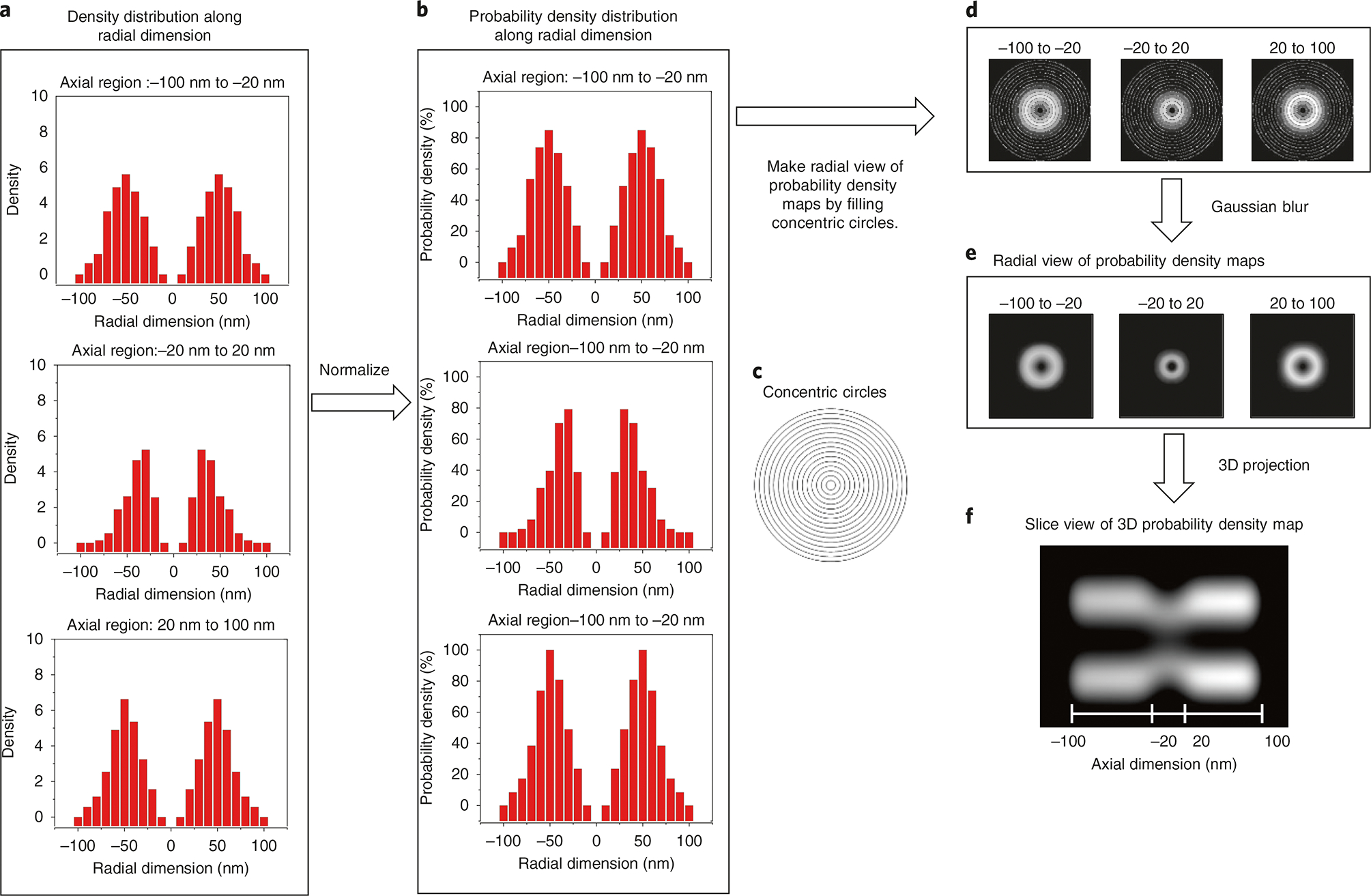
a, Density distribution histograms of the radial dimension within different axial regions. b, Discrete axial region density distribution histograms of the radial dimension normalized to the maximum value density observed within the axial dimension. c, Concentric circles are populated with the probability density distributions to form a radial view of probability density maps. d, Exemplars of preliminary probability density maps. e, Application of a Gaussian blur finalizes the probability density maps of axial regions. f, A section of the composite 3D probability density map. An animation of the composite probability density map is available in the Supplementary Materials.

Parameter	Setting
Projection method	Brightest point
Axis of rotation	y axis
Slice spacing (pixels)	35 or 40 (test both)
Initial angle	0
Total angle	180
Rotation angle increment	10 or 20
Lower transparency	1
Upper transparency	255
Opacity (0–100%)	0
Surface depth cueing (0–100%)	50
Interior depth cueing (0–100%)	50

Check the box for ‘Interpolate’ and click ‘OK’ to obtain the preliminary 3D image stack.

? TROUBLESHOOTING

• 40Select the preliminary 3D image stack. Navigate to ‘Image’ > ‘Type’ > ‘32-bit’. Navigate to ‘Process’ > ‘Filters’ > ‘Gaussian Blur’ to open the ‘Gaussian Blur’ window. Set ‘Sigma (Radius)’ to ‘5–10’ and click ‘OK’ to obtain the final 3D image stack (Fig. 8e,f).

Validation by simulation ● Timing 1–2 h

• 41Install Python 3 and clone or download the ‘Reproducibility Rate’ folder from our GitHub repository at https://github.com/YangLab-Temple/Master.

  ▲CRITICAL STEP Make sure the required Python libraries are installed: tkinter, csv, random, os, sys, numpy, scipy and math. Detailed instructions for installation of Python 3 and the required libraries can be found in our previous publications^47,63.

• 42Run the ‘simulation_gui.py’ file.
• 43
  After the graphical user interface has popped up, modify the default values so that they correspond to the proper experimental parameters (Fig. 7c).

  • ‘# points’ refers to the number of single-molecule localizations.
  • ‘radius (nm)’ refers to the R_I value.
  • ‘precision (nm)’ corresponds to the single-molecule localization precision.
  • ‘# iterations’ refers to the number of R_M values that the simulation will obtain. A higher number of R_M values will minimize the error on the reproducibility rate metric. However, there is often not a practical need to exceed 10,000 for this value.
• 44Click ‘Run simulation’ and allow time for the simulation to run. After completion, the graphical user interface message area will update with the reproducibility rate (Fig. 7c).

Troubleshooting

Troubleshooting advice can be found in Table 2.

Table 2 |.

Troubleshooting table

Steps	Problem	Possible reason	Solution
10B(v)	Too low single-molecule signal or too high fluorescence background when SPEED microscope imaging	The concentration of organic dye-labeling protein is far from the optimal concentration range	To find the optimal concentration, conduct SPEED imaging of a few different concentrations of the labeled protein. We typically use concentrations of 0.1 nM, 0.2 nM, 0.5 nM and 1 nM. Then, we check the single-molecule frequency and background intensity in different concentrations and ensure that individual single molecules are appearing in the field of view separated both spatially and temporally
8	Failure to precisely adjust the laser angle relative to the vertical axis of the sample	It is hard to directly measure the laser angle relative to the vertical axis of the sample	Put a coverslip with cells grown on it on the stage of the microscope and let the laser beam vertically go through the coverslip and the cells. Shift the laser beam off the center of the objective for a distance of d by moving the micrometer stage shown in Fig. 1a. An angle (θ) between the inclined laser beam and the axial direction is formed. The off-center laser beam is reflected by the surface and bottom of the coverslip to have two refection spots, which can be imaged by the camera. The distance (d1) between these two spots can be precisely measured by 2D Gaussian fitting. The relationship between the shifted distance d and the angle θ can be determined by using the formulas $\theta ={\sin }^{-1}\left(\frac{n_{cover}}{n_{cell}}\sin ({\tan }^{-1}\frac{d_1}{l})\right)$ and $d\approx \frac{a*d_1}{l}$ where ncover and ncell are the refractive index of the coverslip and that in cell, respectively, a is the focal length of the objective and l is the thickness of the coverslip
10A(vii)	Poor data quality	The excitation laser power is not within the optimal range. Too high laser power causes rapid photobleaching of molecule, so that it becomes challenging to find a complete nuclear transport event. Too low laser power means that insufficient photons will be collected from the molecule of interest	To find the optimal laser power, excite for the molecule of interest by gradually increasing the laser power from 0.1 mW, 0.2 mW, 0.5 mW and 0.7 mW to 1 mW at the focal plane of the objective. Measure the photobleaching time and collected number of photons from the molecule of interest under different laser powers
10B(iv)	The fluorescent signal cannot be photobleached within 30 s	The power of the photobleaching laser is not high enough, or the molecule diffusion speed is very high	Double the photobleaching laser power or enlarge the photobleaching area (laser spot size at the sample) from 1 to 3 μm (diameter)
11A(iv), B (vii)	Unacceptable shifting of the NE or NPC during imaging	The video recording is too long. Alternatively, accidental vibration of the microscope (for example, as a result of touching the microscope) might cause unacceptable shifting of the NE or NPC	Image the NPC or NE before and after video recording under wide-field laser illumination or mercury lamp. Then, localize and compare the position of the NPC or NE in both images. If shifting is unacceptable, the corresponding videos should be discarded. In our case, acceptable shifting is <10 nm, which is ∼1/20 of the length of the NPC scaffold
40	Generating the 3D projection takes too long	Each individual radial-view density probability map is too big, or the number of rotation angles is too large	(A) Scale down the stack of radial-view density probability maps by using ImageJ: select ‘Image’ > ‘Scale’ > set ‘x scale’ and ‘y scale’ to ‘0.1’, ‘0.2’ or ‘0.5’, set ‘interpolation’ to ‘None’ > uncheck box of ‘Average when downsizing’ and ‘Fill with background color’ > click ‘OK’. The scale of the map should be lower than 600 × 600 pixels. (B) Set ‘Rotation angle increment’ to ‘30’ or ‘60’ when 3D projecting. Thus, the number of rotation angles decreases from 18 or 9 to 6 or 3

Timing

Steps 1–4, cell preparation: 6–7 d

Steps 5–10, SPEED microscopy: 4–5 h

Steps 11–21, 2D data analysis: 3–6 h

Steps 22–40, 2D-to-3D transformation: 1–5 h

Steps 41–44, validation by simulation: 1–2 h

Anticipated results

Upon completion of the SPEED microscopy experiments, the user will have obtained dynamic information at high spatiotemporal resolution by tracking the movement of molecules of interest at the single-molecule level. For example, as shown in Fig. 3a,b, we tracked the nuclear export of single mRNAs through the NPC at a high temporal resolution of 2 ms. These data were used to generate the 2D single-molecule traces through 2D Gaussian function fitting, thereby yielding 2D trajectories of mRNA export (Fig. 3c,d) with a high localization precision of ~8–10 nm³⁹. The 2D trajectories of mRNA transport through the NPC enables the researcher to judge whether mRNAs are exported successfully through the NPCs or aborted. This also enables researchers to determine how long mRNA dwells in the NPC during nuclear export. After collecting hundreds of single-molecule mRNA export trajectories, the nuclear export efficiency of mRNA export, the nuclear export time of mRNA and the diffusion coefficient of mRNA inside and outside the NPCs can be determined³⁹ (Fig. 3e–j). Such dynamic information contributes to our ability to quantitatively characterize nucleocytoplasmic transport mechanism for molecules of interest.

Images containing 2D structural information are acquired by superimposing 2D localizations of molecules of interest from all collected trajectories^33,38,39 (Figs. 3k and 4d–i). The resolution of 2D locations that can be obtained is between 10 and 22 nm, depending on the spatial density of the locations, and is determined by the Fourier ring correlation method^64,65. After analysis of the 2D information, the 2D localizations are run through the 2D-to-3D transformation algorithm to generate 3D probability density maps, which are then overlaid with the structures of interest. 3D probability density maps can be either a composite of the entire structure or smaller sections of interest. Generating the 3D probability density maps and overlaying these with the structure of interest enables us to make several structural conclusions regarding the 3D transport route taken by the molecule of interest as it transits through, and interacts with, the rotationally symmetric structure.

Key examples of different types of results derived from the 2D-to-3D transformation within the NPC were published previously^{33,36,38–40,66,67}. The axial and radial 3D view of the small organic molecules passing through the NPC show that they are highly localized to the axial central channel. This was expected, as molecules smaller than the size-exclusion criteria (<40–60 kDa), such as 10-kDa Alexa Fluor dyes, pass through NPC’s axial central channel³³ (Fig. 4j). When the transport of a nuclear transport receptor importin-β1 (97 kDa) was interrogated, it became clear that the transport receptor does not pass through the center of the central channel. Instead, it passes primarily through the peripheral regions of the central channel, as it must interact with Phe-Gly (FG)-Nups in the process known as facilitated translocation^33,38 (Fig. 4k). The 3D locations of these two distinct nuclear transport mechanisms were revealed by our virtual 3D imaging technique in native NPCs of live cells. Moreover, mapping the configuration of the selectively permeable barrier of the NPC in live cells, which is formed by FG-Nups containing large intrinsically disordered domains, is critical to fully understand the nucleocytoplasmic transport mechanism. By labeling a segment of yeast Nup116 (amino acids 348–458), which is intrinsically disordered and efficiently incorporates into the NPC, we were able to map its interaction sites in the NPC’s permeable barrier by SPEED microscopy and 2D-to-3D transformation. The resulting 3D transformation provides a comprehensive map of FG–FG interactions in the native NPCs and was used to reconstruct the native 3D tomography of the selectively permeable barrier in the NPC³⁶ (Fig. 4g). Different from the above organic dye, cytosol protein and intrinsically disordered protein, we also showed that the membrane-bound protein NET59 translocates to the inner nuclear membrane through the peripheral channels of the NPC³⁸ (Fig. 4l).

This technique is applicable to other rotationally symmetric structures, such as primary cilia and hollow glass nanocapillary (GNC) tubes. For example, we used SPEED microscopy and 2D-to-3D transformation to produce a probability density map that shows the free diffusion of small organic Alexa Fluor dyes throughout the lumen of the hollow GNCs⁴⁰ (Fig. 4o). Lastly, we used SPEED microscopy to study the intraflagellar transport protein IFT20 in the primary cilium. The 3D probability density map shows that IFT20 is localized peripheral to the body of the cilium, where it moves along microtubules for transport within cilia⁴⁰ (Fig. 4n).

Reporting Summary

Further information on research design is available in the Nature Research Reporting Summary linked to this article.

Data availability

The data used to generate example data figures can be found on our lab’s GitHub repository: https://github.com/YangLab-Temple/Data.

Code availability

The code used in this work is available at https://github.com/YangLab-Temple/Master under the GNU General Public License v3.0. Specifically, the code for the reproducibility rate can be found at https://github.com/YangLab-Temple/Master/tree/master/reproducibility%20rate.

References

- 1.Abbe E Beiträge zur Theorie des Mikroskops und der mikroskopischen Wahrnehmung. Archiv für Mik-roskopische Anatomie 9, 413–468 (1873). [Google Scholar]
- 2.Mockl L, Lamb DC & Brauchle C Super-resolved fluorescence microscopy: Nobel Prize in Chemistry 2014 for Eric Betzig, Stefan Hell, and William E. Moerner. Angew. Chem. Int. Ed. Engl. 53, 13972–13977 (2014). [DOI] [PubMed] [Google Scholar]
- 3.Schermelleh L, Heintzmann R & Leonhardt H A guide to super-resolution fluorescence microscopy. J. Cell Biol. 190, 165–175 (2010). [DOI] [PMC free article] [PubMed] [Google Scholar]
- 4.Schermelleh L et al. Super-resolution microscopy demystified. Nat. Cell Biol. 21, 72–84 (2019). [DOI] [PubMed] [Google Scholar]
- 5.Rust MJ, Bates M & Zhuang X Sub-diffraction-limit imaging by stochastic optical reconstruction microscopy (STORM). Nat. Methods 3, 793–796 (2006). [DOI] [PMC free article] [PubMed] [Google Scholar]
- 6.Shroff H, Galbraith CG, Galbraith JA & Betzig E Live-cell photoactivated localization microscopy of nanoscale adhesion dynamics. Nat. Methods 5, 417–423 (2008). [DOI] [PMC free article] [PubMed] [Google Scholar]
- 7.Schnitzbauer J, Strauss MT, Schlichthaerle T, Schueder F & Jungmann R Super-resolution microscopy with DNA-PAINT. Nat. Protoc. 12, 1198–1228 (2017). [DOI] [PubMed] [Google Scholar]
- 8.Kner P, Chhun BB, Griffis ER, Winoto L & Gustafsson MGL Super-resolution video microscopy of live cells by structured illumination. Nat. Methods 6, 339–342 (2009). [DOI] [PMC free article] [PubMed] [Google Scholar]
- 9.Hell SW & Wichmann J Breaking the diffraction resolution limit by stimulated emission: stimulated-emission-depletion fluorescence microscopy. Opt. Lett. 19, 780–782 (1994). [DOI] [PubMed] [Google Scholar]
- 10.Betzig E et al. Imaging intracellular fluorescent proteins at nanometer resolution. Science 313, 1642–1645 (2006). [DOI] [PubMed] [Google Scholar]
- 11.Hess ST, Girirajan TP & Mason MD Ultra-high resolution imaging by fluorescence photoactivation localization microscopy. Biophys. J. 91, 4258–4272 (2006). [DOI] [PMC free article] [PubMed] [Google Scholar]
- 12.Babcock H, Sigal YM & Zhuang X A high-density 3D localization algorithm for stochastic optical reconstruction microscopy. Opt. Nanoscopy 10.1186/2192-2853-1-6 (2012). [DOI] [PMC free article] [PubMed] [Google Scholar]
- 13.von Diezmann A, Shechtman Y & Moerner WE Three-dimensional localization of single molecules for super-resolution imaging and single-particle tracking. Chem. Rev. 117, 7244–7275 (2017). [DOI] [PMC free article] [PubMed] [Google Scholar]
- 14.Fuchs J et al. A photoactivatable marker protein for pulse-chase imaging with superresolution. Nat. Methods 7, 627–630 (2010). [DOI] [PubMed] [Google Scholar]
- 15.Zhu L, Zhang W, Elnatan D & Huang B Faster STORM using compressed sensing. Nat. Methods 9, 721–723 (2012). [DOI] [PMC free article] [PubMed] [Google Scholar]
- 16.Manley S et al. High-density mapping of single-molecule trajectories with photoactivated localization microscopy. Nat. Methods 5, 155–157 (2008). [DOI] [PubMed] [Google Scholar]
- 17.Hoze N et al. Heterogeneity of AMPA receptor trafficking and molecular interactions revealed by superresolution analysis of live cell imaging. Proc. Natl Acad. Sci. USA 109, 17052–17057 (2012). [DOI] [PMC free article] [PubMed] [Google Scholar]
- 18.Yang TT, Tran MNT, Chong WM, Huang CE & Liao JC Single-particle tracking localization microscopy reveals nonaxonemal dynamics of intraflagellar transport proteins at the base of mammalian primary cilia. Mol. Biol. Cell 30, 828–837 (2019). [DOI] [PMC free article] [PubMed] [Google Scholar]
- 19.Izeddin I et al. Wavelet analysis for single molecule localization microscopy. Opt. Express 20, 2081–2095 (2012). [DOI] [PubMed] [Google Scholar]
- 20.Gustafsson MG Surpassing the lateral resolution limit by a factor of two using structured illumination microscopy. J. Microsc. 198, 82–87 (2000). [DOI] [PubMed] [Google Scholar]
- 21.Heintzmann R & Cremer CG in Optical Biopsies and Microscopic Techniques III 185–196 (International Society for Optics and Photonics, 1999). [Google Scholar]
- 22.Gustafsson MG et al. Three-dimensional resolution doubling in wide-field fluorescence microscopy by structured illumination. Biophys. J. 94, 4957–4970 (2008). [DOI] [PMC free article] [PubMed] [Google Scholar]
- 23.Schermelleh L et al. Subdiffraction multicolor imaging of the nuclear periphery with 3D structured illumination microscopy. Science 320, 1332–1336 (2008). [DOI] [PMC free article] [PubMed] [Google Scholar]
- 24.Heintzmann R & Ficz G Breaking the resolution limit in light microscopy. Brief. Funct. Genomic. Proteomic. 5, 289–301 (2006). [DOI] [PubMed] [Google Scholar]
- 25.Vicidomini G, Bianchini P & Diaspro A STED super-resolved microscopy. Nat. Methods 15, 173–182 (2018). [DOI] [PubMed] [Google Scholar]
- 26.Westphal V, Lauterbach MA, Di Nicola A & Hell SW Dynamic far-field fluorescence nanoscopy. N. J. Phys. 9, 435–435 (2007). [Google Scholar]
- 27.Willig K, Keller J, Bossi M & Hell SW STED microscopy resolves nanoparticle assemblies. N. J. Phys. 8, 106 (2006). [Google Scholar]
- 28.Willig KI, Rizzoli SO, Westphal V, Jahn R & Hell SW STED microscopy reveals that synaptotagmin remains clustered after synaptic vesicle exocytosis. Nature 440, 935–939 (2006). [DOI] [PubMed] [Google Scholar]
- 29.Dyba M & Hell SW Focal spots of size lambda/23 open up far-field florescence microscopy at 33 nm axial resolution. Phys. Rev. Lett. 88, 163901 (2002). [DOI] [PubMed] [Google Scholar]
- 30.Dyba M, Jakobs S & Hell SW Immunofluorescence stimulated emission depletion microscopy. Nat. Biotechnol. 21, 1303–1304 (2003). [DOI] [PubMed] [Google Scholar]
- 31.Dyba M, Keller J & Hell SW Phase filter enhanced STED-4Pi fluorescence microscopy: theory and experiment. N. J. Phys. 7, 134–134 (2005). [Google Scholar]
- 32.Klar TA, Jakobs S, Dyba M, Egner A & Hell SW Fluorescence microscopy with diffraction resolution barrier broken by stimulated emission. Proc. Natl Acad. Sci. USA 97, 8206–8210 (2000). [DOI] [PMC free article] [PubMed] [Google Scholar]
- 33.Sidenstein SC et al. Multicolour multilevel STED nanoscopy of actin/spectrin organization at synapses. Sci. Rep. 6, 26725 (2016). [DOI] [PMC free article] [PubMed] [Google Scholar]
- 34.Kilian N et al. Assessing photodamage in live-cell STED microscopy. Nat. Methods 15, 755–756 (2018). [DOI] [PMC free article] [PubMed] [Google Scholar]
- 35.Lauterbach MA et al. Comparing video-rate STED nanoscopy and confocal microscopy of living neurons. J. Biophotonics 3, 417–424 (2010). [DOI] [PubMed] [Google Scholar]
- 36.Pellett PA et al. Two-color STED microscopy in living cells. Biomed. Opt. Express 2, 2364–2371 (2011). [DOI] [PMC free article] [PubMed] [Google Scholar]
- 37.Gwosch KC et al. MINFLUX nanoscopy delivers 3D multicolor nanometer resolution in cells. Nat. Methods 17, 217–224 (2020). [DOI] [PubMed] [Google Scholar]
- 38.Ma J & Yang W Three-dimensional distribution of transient interactions in the nuclear pore complex obtained from single-molecule snapshots. Proc. Natl Acad. Sci. USA 107, 7305–7310 (2010). [DOI] [PMC free article] [PubMed] [Google Scholar]
- 39.Goryaynov A, Ma J & Yang W Single-molecule studies of nucleocytoplasmic transport: from one dimension to three dimensions. Integr. Biol. 4, 10–21 (2012). [DOI] [PMC free article] [PubMed] [Google Scholar]
- 40.Goryaynov A & Yang W Role of molecular charge in nucleocytoplasmic transport. PLoS ONE 9, e88792 (2014). [DOI] [PMC free article] [PubMed] [Google Scholar]
- 41.Junod SL, Kelich JM, Ma J & Yang W Nucleocytoplasmic transport of intrinsically disordered proteins studied by high-speed super-resolution microscopy. Protein Sci. 29, 1459–1472 (2020). [DOI] [PMC free article] [PubMed] [Google Scholar]
- 42.Luo W et al. Axonemal lumen dominates cytosolic protein diffusion inside the primary cilium. Sci. Rep. 7, 1–11 (2017). [DOI] [PMC free article] [PubMed] [Google Scholar]
- 43.Ma J, Goryaynov A, Sarma A & Yang W Self-regulated viscous channel in the nuclear pore complex. Proc. Natl Acad. Sci. USA 109, 7326–7331 (2012). [DOI] [PMC free article] [PubMed] [Google Scholar]
- 44.Ma J, Goryaynov A & Yang W Super-resolution 3D tomography of interactions and competition in the nuclear pore complex. Nat. Struct. Mol. Biol. 23, 239–247 (2016). [DOI] [PMC free article] [PubMed] [Google Scholar]
- 45.Ma J et al. High-resolution three-dimensional mapping of mRNA export through the nuclear pore. Nat. Commun. 4, 1–9 (2013). [DOI] [PMC free article] [PubMed] [Google Scholar]
- 46.Mudumbi KC et al. Nucleoplasmic signals promote directed transmembrane protein import simultaneously via multiple channels of nuclear pores. Nat. Commun. 11, 1–14 (2020). [DOI] [PMC free article] [PubMed] [Google Scholar]
- 47.Westphal V et al. Video-rate far-field optical nanoscopy dissects synaptic vesicle movement. Science 320, 246–249 (2008). [DOI] [PubMed] [Google Scholar]
- 48.Li Y, Luo W & Yang W Nuclear transport and accumulation of smad proteins studied by single-molecule microscopy. Biophys. J. 114, 2243–2251 (2018). [DOI] [PMC free article] [PubMed] [Google Scholar]
- 49.Sun C, Yang W, Tu L-C & Musser SM Single-molecule measurements of importin α/cargo complex dissociation at the nuclear pore. Proc. Natl Acad. Sci. USA 105, 8613–8618 (2008). [DOI] [PMC free article] [PubMed] [Google Scholar]
- 50.Yang W & Musser SM Visualizing single molecules interacting with nuclear pore complexes by narrow-field epifluorescence microscopy. Methods 39, 316–328 (2006). [DOI] [PMC free article] [PubMed] [Google Scholar]
- 51.Solovei I et al. LBR and lamin A/C sequentially tether peripheral heterochromatin and inversely regulate differentiation. Cell 152, 584–598 (2013). [DOI] [PubMed] [Google Scholar]
- 52.Mudumbi KC, Yang W, Ma J & Schirmer EC Single-point frap distinguishes inner and outer nuclear membrane protein distribution. Biophys. J. 110, 596a (2016). [DOI] [PMC free article] [PubMed] [Google Scholar]
- 53.Daigle N et al. Nuclear pore complexes form immobile networks and have a very low turnover in live mammalian cells. J. Cell Biol. 154, 71–84 (2001). [DOI] [PMC free article] [PubMed] [Google Scholar]
- 54.Feldherr CM, Kallenbach E & Schultz N Movement of a karyophilic protein through the nuclear pores of oocytes. J. Cell Biol. 99, 2216–2222 (1984). [DOI] [PMC free article] [PubMed] [Google Scholar]
- 55.Kubitscheck U, Wedekind P, Zeidler O, Grote M & Peters R Single nuclear pores visualized by confocal microscopy and image processing. Biophys. J. 70, 2067–2077 (1996).TOCOL [DOI] [PMC free article] [PubMed] [Google Scholar]
- 56.Tokunaga M, Imamoto N & Sakata-Sogawa K Highly inclined thin illumination enables clear single-molecule imaging in cells. Nat. Methods 5, 159–161 (2008). [DOI] [PubMed] [Google Scholar]
- 57.Mudumbi KC, Schirmer EC & Yang W Single-point single-molecule FRAP distinguishes inner and outer nuclear membrane protein distribution. Nat. Commun. 7, 1–6 (2016). [DOI] [PMC free article] [PubMed] [Google Scholar]
- 58.Tingey M, Mudumbi KC, Schirmer EC & Yang W Casting a wider net: differentiating between inner nuclear envelope and outer nuclear envelope transmembrane proteins. Int. J. Mol. Sci. 20, 5248 (2019). [DOI] [PMC free article] [PubMed] [Google Scholar]
- 59.Ott C & Lippincott-Schwartz J Visualization of live primary cilia dynamics using fluorescence microscopy. Curr. Protoc. Cell Biol. Chapter 4, Unit 4 26 (2012). [DOI] [PMC free article] [PubMed] [Google Scholar]
- 60.Schindelin J et al. Fiji: an open-source platform for biological-image analysis. Nat. Methods 9, 676–682 (2012). [DOI] [PMC free article] [PubMed] [Google Scholar]
- 61.Grünwald D & Singer RH In vivo imaging of labelled endogenous β-actin mRNA during nucleocytoplasmic transport. Nature 467, 604–607 (2010). [DOI] [PMC free article] [PubMed] [Google Scholar]
- 62.Herbert A Single Molecule Light Microscopy ImageJ Plugins. http://www.sussex.ac.uk/gdsc/intranet/pdfs/SMLM.pdf (2014).
- 63.Punge A et al. 3D reconstruction of high-resolution STED microscope images. Microsc. Res. Tech. 71, 644–650 (2008). [DOI] [PubMed] [Google Scholar]
- 64.Banterle N, Bui KH, Lemke EA & Beck M Fourier ring correlation as a resolution criterion for superresolution microscopy. J. Struct. Biol. 183, 363–367 (2013). [DOI] [PubMed] [Google Scholar]
- 65.Nieuwenhuizen RP et al. Measuring image resolution in optical nanoscopy. Nat. Methods 10, 557–562 (2013). [DOI] [PMC free article] [PubMed] [Google Scholar]
- 66.Giannone G et al. Dynamic superresolution imaging of endogenous proteins on living cells at ultra-high density. Biophys. J. 99, 1303–1310 (2010). [DOI] [PMC free article] [PubMed] [Google Scholar]
- 67.Agasti SS et al. DNA-barcoded labeling probes for highly multiplexed Exchange-PAINT imaging. Chem. Sci. 8, 3080–3091 (2017). [DOI] [PMC free article] [PubMed] [Google Scholar]
- 68.Bates M, Blosser TR & Zhuang X Short-range spectroscopic ruler based on a single-molecule optical switch. Phys. Rev. Lett. 94, 108101 (2005). [DOI] [PMC free article] [PubMed] [Google Scholar]
- 69.Bates M et al. in Single Molecule Spectroscopy in Chemistry, Physics and Biology 399–415 (Springer, 2010). [Google Scholar]
- 70.Gordon MP, Ha T & Selvin PR Single-molecule high-resolution imaging with photobleaching. Proc. Natl Acad. Sci. USA 101, 6462–6465 (2004). [DOI] [PMC free article] [PubMed] [Google Scholar]
- 71.Heilemann M, Margeat E, Kasper R, Sauer M & Tinnefeld P Carbocyanine dyes as efficient reversible single-molecule optical switch. J. Am. Chem. Soc. 127, 3801–3806 (2005). [DOI] [PubMed] [Google Scholar]
- 72.Kubitscheck U et al. Nuclear transport of single molecules: dwell times at the nuclear pore complex. J. Cell Biol. 168, 233–243 (2005). [DOI] [PMC free article] [PubMed] [Google Scholar]
- 73.Ober RJ, Ram S & Ward ES Localization accuracy in single-molecule microscopy. Biophys. J. 86, 1185–1200 (2004). [DOI] [PMC free article] [PubMed] [Google Scholar]
- 74.Qu X, Wu D, Mets L & Scherer NF Nanometer-localized multiple single-molecule fluorescence microscopy. Proc. Natl Acad. Sci. USA 101, 11298–11303 (2004). [DOI] [PMC free article] [PubMed] [Google Scholar]
- 75.Owen DM, Williamson D, Magenau A, Rossy J & Gaus K in Methods in Enzymology Vol. 504 221–235 (Elsevier, 2012). [DOI] [PubMed] [Google Scholar]
- 76.York AG, Ghitani A, Vaziri A, Davidson MW & Shroff H Confined activation and subdiffractive localization enables whole-cell PALM with genetically expressed probes. Nat. Methods 8, 327–333 (2011). [DOI] [PMC free article] [PubMed] [Google Scholar]
- 77.Temprine K, York AG & Shroff H Three-dimensional photoactivated localization microscopy with genetically expressed probes. Methods Mol. Biol. 1251, 231–261 (2015). [DOI] [PMC free article] [PubMed] [Google Scholar]
- 78.Sharonov A & Hochstrasser RM Wide-field subdiffraction imaging by accumulated binding of diffusing probes. Proc. Natl Acad. Sci. USA 103, 18911–18916 (2006). [DOI] [PMC free article] [PubMed] [Google Scholar]
- 79.Jungmann R et al. Multiplexed 3D cellular super-resolution imaging with DNA-PAINT and Exchange-PAINT. Nat. Methods 11, 313–318 (2014). [DOI] [PMC free article] [PubMed] [Google Scholar]
- 80.Iinuma R et al. Polyhedra self-assembled from DNA tripods and characterized with 3D DNA-PAINT. Science 344, 65–69 (2014). [DOI] [PMC free article] [PubMed] [Google Scholar]
- 81.Schueder F et al. Multiplexed 3D super-resolution imaging of whole cells using spinning disk confocal microscopy and DNA-PAINT. Nat. Commun. 8, 1–9 (2017). [DOI] [PMC free article] [PubMed] [Google Scholar]
- 82.Lin R, Clowsley AH, Lutz T, Baddeley D & Soeller C 3D super-resolution microscopy performance and quantitative analysis assessment using DNA-PAINT and DNA origami test samples. Methods 174, 56–71 (2020). [DOI] [PubMed] [Google Scholar]
- 83.Strauss S et al. Modified aptamers enable quantitative sub-10-nm cellular DNA-PAINT imaging. Nat. Methods 15, 685–688 (2018). [DOI] [PMC free article] [PubMed] [Google Scholar]
- 84.Nieves DJ, Gaus K & Baker MA DNA-based super-resolution microscopy: DNA-PAINT. Genes 9, 621 (2018). [DOI] [PMC free article] [PubMed] [Google Scholar]
- 85.Chung E, Kim D & So PT Extended resolution wide-field optical imaging: objective-launched standing-wave total internal reflection fluorescence microscopy. Opt. Lett. 31, 945–947 (2006). [DOI] [PubMed] [Google Scholar]
- 86.Richter V, Piper M, Wagner M & Schneckenburger H Increasing resolution in live cell microscopy by structured illumination (SIM). Appl. Sci. 9, 1188 (2019). [Google Scholar]
- 87.Förster R et al. Simple structured illumination microscope setup with high acquisition speed by using a spatial light modulator. Opt. Express 22, 20663–20677 (2014). [DOI] [PubMed] [Google Scholar]
- 88.Strohl F & Kaminski CF Speed limits of structured illumination microscopy. Opt. Lett. 42, 2511–2514 (2017). [DOI] [PubMed] [Google Scholar]
- 89.Schmidt R et al. Spherical nanosized focal spot unravels the interior of cells. Nat. Methods 5, 539–544 (2008). [DOI] [PubMed] [Google Scholar]
- 90.Hell SW Toward fluorescence nanoscopy. Nat. Biotechnol. 21, 1347–1355 (2003). [DOI] [PubMed] [Google Scholar]
- 91.Manley S, Gillette JM & Lippincott-Schwartz J in Methods in Enzymology Vol. 475 109–120 (Elsevier, 2010). [DOI] [PMC free article] [PubMed] [Google Scholar]
- 92.Subach FV, Patterson GH, Renz M, Lippincott-Schwartz J & Verkhusha VV Bright monomeric photoactivatable red fluorescent protein for two-color super-resolution sptPALM of live cells. J. Am. Chem. Soc. 132, 6481–6491 (2010). [DOI] [PMC free article] [PubMed] [Google Scholar]
- 93.Ruba A, Luo W, Kelich J, Tingey M & Yang W 3D tracking-free approach for obtaining 3D super-resolution information in rotationally symmetric biostructures. J. Phys. Chem. B 123, 5107–5120 (2019). [DOI] [PMC free article] [PubMed] [Google Scholar]
Associated Data
This section collects any data citations, data availability statements, or supplementary materials included in this article.
Supplementary Materials
Data Availability Statement