

Abstract
Complex interactions between genes determine the development and differentiation of cells. We establish a landscape theory for cell differentiation with proliferation effect, in which the developmental process is modeled as a stochastic dynamical system with a birth-death term. We find that two different energy landscapes, denoted U and V, collectively contribute to the establishment of non-equilibrium steady differentiation. The potential U is known as the energy landscape leading to the steady distribution, whose metastable states stand for cell types, while V indicates the differentiation direction from pluripotent to differentiated cells. This interpretation of cell differentiation is different from the previous landscape theory without the proliferation effect. We propose feasible numerical methods and a mean-field approximation for constructing landscapes U and V. Successful applications to typical biological models demonstrate the energy landscape decomposition's validity and reveal biological insights into the considered processes.
Keywords: energy landscape, cell differentiation, stochastic systems
Energy landscape decomposition (ELD) theory provides a computational tool to construct epigenetic and pluripotency landscapes for cell differentiation process with proliferation effect.
INTRODUCTION
Cell differentiation makes the biological world rich and colorful. Modeling and understanding the dynamics of gene regulatory networks (GRNs) are essential to explore the underlying mechanism of cell differentiation [1]. Since Waddington proposed his seminal metaphor of the epigenetic landscape [2,3], differentiation has been intuitively described as a ball rolling down a surface, i.e. the energy landscape.
There are mainly two approaches to construct the energy landscape for biosystems. One is the data-based approach, which tries to identify cluster/cell types, differentiation trajectories, pseudotime and cell pluripotency from the experimental data, especially single-cell RNA sequencing (scRNA-seq) data [4–8]. Various algorithms have been proposed from the theory of graph [9,10], entropy [6,11,12] and dynamical systems [13–16]. Among these data-based methods, the population balance analysis (PBA) [13–15] and landscape of differentiation dynamics (LDD) [16] especially involve cell proliferation and death rates, which generalize the hypothesis of cell differentiation from equilibrium to non-equilibrium steady processes. The other approach is the model-based approach, which tries to build dynamic equations from the GRN, analyze the dynamical behavior of the system and then construct energy landscapes using numerical simulations. Wang et al. proposed a practical framework for constructing energy landscapes for biosystems without cell birth and death effects [17–19]. They defined the landscape as  , where
  is the gene expression vector,
  is the steady probability density function (PDF) of the system and ε is related to the amplitude of small intrinsic noise. By changing parameter values to control the biological process, the landscape pattern varies, which gives an intuitive description of cell-type locations and transition probability between clusters. This framework has been widely used in modeling the budding yeast cell cycle [17], human stem cell fate [19] and Caenorhabditis elegans ageing [20]. Without the cell proliferation effect, however, the direction of differentiation is usually not intrinsic in Wang’s landscape but controlled by manually setting parameters. Beyond the topics above, there are also many other interesting works related to the energy landscape theory [21–27].
In this study, we follow the model-based approach but consider the birth and death rates (BDRs) of cells in differentiation, which is inspired by the PBA and LDD. We show that there are two important energy landscapes to describe differentiation dynamics, which are denoted  and
and  and are also computable using the model. The metastable states in
  represent cell types, and the value of
  implicates pluripotency. The negative gradient of
  shows the direction of differentiation. Taking BDRs into account is essential for constructing the pluripotency landscape
  . Here, we explain our theory of the energy landscape decomposition (ELD) in cell differentiation with proliferation effect. Numerical algorithms for constructing energy landscapes and the mean-field approximation (MFA) in high-dimensional cases are also proposed. We use three examples to show the application of the ELD, where
  and
and  intuitively explain the processes of cell differentiation.
RESULTS
Modeling cell differentiation at the population level
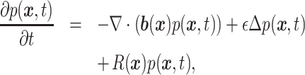
Motivated by Weinreb et al. [13] and Briggs et al. [15], we modeled cell development through a stochastic dynamical system with the birth-death term. We denote gene expression levels using  . During cell differentiation, the cell population is quantified using a PDF
  , whose evolution follows a generalized form of the well-known Fokker-Planck equation (FPE), i.e.
 |
(1) |
with an initial PDF  at t = 0, where
  represents the biological interactions between genes, ε is a parameter standing for the noise amplitude and
  stands for the net BDR of cells at
  . In a practical application,
  is usually modeled using either activated or inhibited Hill functions, according to the considered GRN. Here
  indicates the proliferation of cells, while
  indicates the death of cells. When
  , (1) reduces to the standard FPE without any cell proliferation effect. To ensure a non-explosive and non-degenerative steady PDF
  for (1), we require the following condition as a constraint for
  :
:
 |
(2) |
It is necessary to have a non-trivial  to characterize the population balance of the cell birth and death in the steady state.
Modeling cell differentiation at the single-cell level
The population-level dynamics in (1) can also be viewed as the probabilistic interpretation at the single-cell level. We consider a cell ω with gene expression  starting from
  at t = 0 and propose a weighted stochastic dynamics in the Itô sense as
 |
(3a) |
 |
(3b) |
 |
(3c) |
 |
(3d) |
where  is distributed according to
  ,
,  is a standard Brownian motion with independent components and ρt(ω) stands for a time-varying weight for cell ω. The connection between (1) and (3) is represented as
 |
(4) |
where δ is the Dirac delta function and the expectation is taken over all the possible trajectories ω (see the online supplementary material for details). The weight ρt(ω) increases at t when  , which corresponds to cell proliferation, while it decreases at t when
  , which corresponds to cell death. If
  , the weight ρt(ω) is a constant for every cell and the system reduces to the case without any cell proliferation, which is discussed by Wang et al. [17,18].
Energy landscape decomposition
Based on the above dynamical modeling of cell development, we focus on the construction of the landscapes using the model-based approach, i.e. we assume that  , and
, and  are known a priori.
We denote by  the steady PDF with the known BDR
  and by
  the steady PDF with
  , for (1). Note that the notation
  is different from the initial distribution
  . Then, two energy landscapes are constructed as
 |
(5) |
which drives the system or cells to the steady distribution, and
 |
(6) |
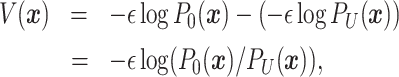
which quantifies the change of the potential caused by  , i.e. the influence induced by cell proliferation and death. The metastable basins in landscape
  indicate cell types, and the depth of each basin characterizes its stability. The values of V depict the pluripotency and its negative gradient field describes the differentiation direction. From a stem cell state to a differentiated cell state, V decreases gradually. The potential U is the cell-type landscape and V is the pluripotency landscape. Besides the two potential functions, the remaining term
  is defined as
 |
(7) |
which is the curl part that describes the non-gradientness of the considered dynamics. The  term satisfies
 |
(8) |
which corresponds to the divergence-free condition of the curl flux  defined in [17,18].
In summary, we propose an energy decomposition for the differentiation dynamics characterized by the pair  in our ELD framework as
 |
(9) |
The potentials U and V, together with the curl part  , help us have a deep understanding of cell differentiation and cell subtypes along the differentiation pathway. Figure 1 presents an illustration of the whole ELD procedure.
Figure 1.

An illustration of the ELD framework. (a) The GRN, which reins cell differentiation dynamics. Dynamical flow  can be modeled using the GRN, and its vector field is drawn in an illustrative space (X, Y). (b) Cells can proliferate or die at a natural birth and death rate
  . Proliferation with
  is shown in red, while cell death with
  is in blue (jet colormap). (c) The ELD theory in this study. The dynamics
  can be characterized using two potential terms (energy landscapes)
  and
and  , and a curl part term
  . We define
  and
and  using two steady PDFs, denoted
  and
and  . (d) The combination of dynamical flow
  (arrows) and birth and death rate
  (jet colored background). (e–g) Illustrations for the cell-type landscape
  , the pluripotency landscape
  and the curl part term
  , respectively. Metastable states of
  shown in (e) stand for different cell types. The values of
  shown in (f) indicate the pluripotency, with its negative gradient depicting the differentiation direction. The color bar in (f) is calculated using the mean value of V along the X axis, which displays an intuitive global differentiation direction. In (g), landscape
  is plotted as the background, while the curl part term
  is indicated by the vectors.
The connection between the ELD framework and the existing landscape theory is as follows. In the case of no birth and death of cells, i.e.  , (9) reduces to Wang’s landscape decomposition [17–19] with
  and
and  ; if the system is of gradient type with
  , (9) reduces to the landscape decomposition discussed in PBA and LDD [13,16] with
  .
.
In a case that only  is known, PBA and LDD define the energy landscape V for gradient systems by solving the equation
 |
(10) |
with proper boundary conditions. However, for a non-gradient system, we show that (10) is not always valid, unless the curl part  satisfies
  almost everywhere (see the online supplementary material for details). In this sense, we provide a more general definition of V using (6). More detailed discussion about the ELD can be found in the online supplementary material.
Numerical construction of energy landscapes
According to the definitions of potentials  in (5) and
  in (6), we can compute the energy landscapes once the steady distributions
  and
and  are obtained. Next we discuss the numerical methods for the low-dimensional case and the high-dimensional case separately.
Solving FPE for the low-dimensional case
For the low-dimensional case (usually in less than three dimensions), we used the finite difference or finite element method to solve (1) numerically until the steady state. For a small parameter ε, the spatial scale h of the grids in traditional methods is needed to be set as h ≪ ε to resolve the dynamical behavior of such a convection-dominated equation, which would be impractical. We utilized the streamline diffusion method [28] that can avoid the numerical oscillations even when h > ε. The detailed procedure of the streamline diffusion method is described in the online supplementary material in a two-dimensional case. It is also applied in our numerical examples in the Results section.
Mean-field approximation in the high-dimensional case
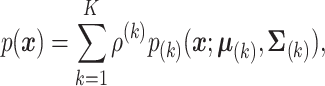
For the high-dimensional case, it is not feasible to directly solve (1). Thus, we start from the single-cell dynamics (3) and propose an MFA approach to reduce the computational complexity from exponential to polynomial time. Overall, the potentials PU and P0 are approximated by the Gaussian mixtures in the MFA, i.e.
 |
(11) |
where K is the number of components obtained by the counts of stable states in the deterministic dynamics  ,
, 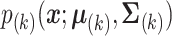 is the kth Gaussian component with mean
  and covariance
  , and ρ(k) is the mixture weight. These approximations are obtained through asymptotics of (3) with respect to the small parameter ε.
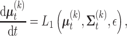
Short time asymptotics. We denote by Ωk the kth attractive basin for the  dynamics in (3). In the O(1) timescale (or the transition timescale in Ωk), there is no state hopping and we derive the approximation
  , where
  when the initial
  . The mean and covariance satisfy the equations
 |
(12a) |
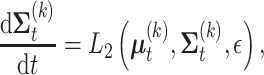 |
(12b) |
where L1 and L2 are functions derived from the Taylor expansion of  around
  until O(ε) terms. The details are shown in the online supplementary material. The parameters
  are steady states of (12). Especially,
  in the O(1) approximation (i.e. ε = 0) and we recover the classical MFA [17,29].
Long time asymptotics. The determination of the mixture weights {ρ(k)} is designed to take into account the basin transitions in a longer time scale like log (t) ≳ O(1/ε). In this regime, the diffusion dynamics of  is upscaled to a continuous-time Markov chain, in which the Arrhenius-type transition rates depend on the energy barriers between the corresponding attraction basins [30,31]. We assume that the upscaled transition rate matrix is
  and define
  as the average BDR. The evolution of weights
  with/without a birth-death term
  shows the asymptotics
 |
(13) |
where  ,
,  is the mixture weights for
  and
and  is the mixture weights for
  . As accurate
  is difficult to obtain, we perform a Monte Carlo approximation to steady
  by utilizing the equation
 |
(14) |
where the trajectories are simulated with a uniform initial distribution on a finite domain at t = 0 until a suitable finite ending time t = T. Such a choice actually gives the same MFA as proposed in [17,18] without the  term. With ergodic assumption, the steady mixture weights
  for
for  are derived as
 |
(15) |
where qk = −Qkk is the exit rate for state k. Under the constraint equation, (2), and an additional assumption that  , an approximation for qk and thus
  is also obtained (see the online supplementary material for details).
With the mean-field approximations  and
and  , we obtain the estimations for the landscapes
  and
and  using (5) and (6), respectively.
Several detailed remarks need to be made. (i) There is also an MFA to (1), but, for multi-potential systems, the MFA to (1) can have different numbers of components with different parameters when approximating  and
and  , respectively. That can lead to an odd
  . Thus, one of the advantages of the MFA to (3) is that the numbers of components K and
  computed using (12) are independent of the BDR
  , and only mixture weights estimated in (14) and (15) are different. (ii) The MFA to (3) is not suitable for monostable systems, as the mixture weight for trajectories in the only attractive basin is supposed to be the same. For the system with a uni-component, we use the MFA to (3), which is also described in detail in the online supplementary material. For real problems, most systems are multi-stable with several different components. (iii) In (12), the MFA is expanded to O(ε) in functions L1 and L2. In Wang’s framework [17,18] where
  , it is only expanded to O(1) to estimate energy landscape
  . In the online supplementary material, we state that it is necessary to have the MFA to O(ε) to obtain a proper approximation of
  . Two analytic examples are also used to validate the necessity.
Numerical examples
In this section, we utilize three examples to show how we applied the ELD framework to describe cell differentiation.
Example 1: two-dimensional drift-diffusion process
For the first example, we use a two-dimensional drift-diffusion process as a basic example for simulating cell differentiation [13,16]. In this example, we take  to be a gradient field with
 |
(16) |
and set the rate function  , where
  . The noise parameter is ε = 0.01. There exist three stable equilibrium points of the potential
  , i.e.
  ,
,  and
and  , which correspond to three cell types. According to
  , most cells proliferate around
  , and die around
  and
and  . Thus, cell type A around
  stands for stem cells with high pluripotency, while cell types B around
  and C around
  represent differentiated states. Using the streamline diffusion method to solve (1) with and without
  , we obtain the distributions PU and P0, respectively. Furthermore, the energy landscapes U and V are constructed as shown in Fig. 2. Three cell types are easily identified in
  . The effect of the birth and death rate
  determines the differentiation direction of the process, and the values of
  characterize the stemness from high to low. Figure S1 within online supplementary material also shows the original potential
  , together with the two-dimensional projections of U and V.
Figure 2.

The landscapes for the two-dimensional drift-diffusion process. (a) The landscape U. Three metastable states represent three cell types. (b) The landscape V. The cells differentiate from the state at a high value of V to a lower value.
Example 2: the two-gene fate decision system
The second example models a binary cell fate decision controlled by the interaction between two genes [18,32,33]. Figure 3a shows the regulatory relationships between the two genes. It is modeled using a non-gradient Hill dynamics as
 |
(17) |
where the parameters are set as α1 = α2 = 0.3, β1 = β2 = 0.5, n = 4, k1 = k2 = 1 and S = 0.5. Through self-activation and inter-inhibition, the two genes X1 and X2 (such as GATA1 and PU.1) are coexpressed in the pluripotent stem cell, and one gene gradually dominates over the other when the system is committed to two different lineages. In Wang’s framework, α1, α2, β1 and β2 vary to control the differentiation [18]. However, in the current viewpoint of cell differentiation, ELD theory claims that, even if these parameters are fixed, the cell fate decision can be adjusted according to the change in BDR  . To construct the landscapes U and V, we set the noise amplitude ε = 0.01, and the birth and death rate
  . The rate amplitude r is changed from 30 to 0. Figure 3c and d demonstrate how the landscapes change when r decreases, and Fig. 3b shows the landscape of U when r = 0 (the landscape V ≡ 0). We obtain the following results through our computations: (i) when the BDR is high (r = 30), there is only one cell type characterized by U, where X1 and X2 are coexpressed; (ii) this single state splits into two as the amplitude of BDR decreases, i.e. differentiation; (iii) in the two separated cell types when r = 0, one gene dominates over the other; (iv) the value of V characterizes the pluripotency of cells, and −∇V indicates the differentiation direction. Overall, instead of changing the interaction strength between genes, the BDR term
  might also be responsible for explaining cell differentiation, which controls the cell fate decision.
Figure 3.

(a) The interaction between two genes X1 and X2 in the fate decision system. Self-activation and inter-inhibition are observed. (b) The landscape U when the amplitude of the birth and death rate is set as r = 0. (c) The landscape U changes when r decreases from 30 to 3. (d) The landscape V changes when r decreases from 30 to 3.
Example 3: T-cell differentiation
The third example is used to describe the T-cell differentiation in high-dimensional space [34]. Four genes x1 (TCF-1), x2 (PU.1), x3 (GATA3) and x4 (BLC11B) interact with each other through activation or inhibition (see Fig. 4a). The dynamical term  is modeled using Hill functions and the parameters are listed in the online supplementary material. We set the BDR as
  . Using the MFA equation, (11), the landscapes are constructed as shown in Fig. 4b and c. The potential U corresponds to the steady-state landscape with birth-death term R. The four metastable states stand for the four stages of development of T cells (ETP/DN1, DN2a, DN2b and DN3). The potential V in Fig. 4c shows the pluripotency of cells with its value and differentiation direction with its negative gradient field. As applied to MFA, the BDR is also averaged for each Gaussian component, so the variation of
  within each metastable state/cell type is much smaller than that shown by U. Accordingly, there exists a sharp variation of V between two adjacent cell types, as shown in Fig. 4c.
Figure 4.

(a) The gene regulatory network in the T-cell differentiation process. The four genes X1, X2, X3 and X4 are TCF-1, PU.1, GATA3 and BLC11B, respectively. (b) The landscape U and (c) the landscape V. Metastable states represent the T-cell stages, i.e. ETP/DN1, DN2a, DN2b and DN3. The potential V indicates the pluripotency and differentiation direction.
Besides the four-dimensional example for T-cell differentiation, we also conducted ELD on a high-dimensional example with 10 variables shown in Sec. IV(D) and Figure S2 of the online supplementary material. These results support the fact that the ELD and MFA are practical in studying the metastable states by energy landscape U and the pluripotency by energy landscape V.
CONCLUSIONS AND DISCUSSIONS
In this paper, we have proposed the ELD framework to describe cell differentiation with proliferation effect. Two energy landscapes,  and
and  , can explain the dynamical behavior of the system during differentiation. The potential U depicts the attractors standing for cell types, while V characterizes the pluripotency and differentiation direction. The consideration of BDR is important to construct V. With an additional V, ELD theory is a generalization of traditional energy landscape theory, and it is a natural realization for Waddington’s epigenetic landscape with birth-death terms. The numerical construction of ELD, especially its mean-field approximation in high-dimensional cases, is introduced. Simulated examples demonstrate the applicability of ELD. However, there are still several issues that need to be further discussed and studied.
First, the ELD framework is different from other models for constructing landscapes for cell differentiation. PBA and LDD are data driven, which are based on the scRNA-seq data and difficult to handle the non-gradient system. Wang’s landscape does not consider the birth and death of cells during the differentiation. ELD is model based and analyzes a landscape V caused by cell proliferation and death to display the differentiation direction.
Second, the BDR  in our model is known a priori. For practical cases, R can be estimated from experiments (as in PBA, [13]) or approximated for each cell type (as in LDD, [16]). If only R for cell types matters, which means that R is a constant for each metastable state, the corresponding V will change little within one state while varying sharply between two adjacent states.
Third, the estimated mixture weights  in (14) are only rough approximations according to the size of attractive basins (percentages of trajectories falling into one meta-stable state). A more rational approach is to get the transition rate matrix
  between different states [31,35–37]. However, it is difficult to catch rare transitions within the limited time of the simulation. A quick and accurate way to estimate mixture weights is still an open question.
Fourth, constructing landscapes for systems with limit cycles is also possible once a proper BDR is given. According to the approximation in [17],  can be used as the kth component in (11), where T is the period for the limit cycle and
  is the Gaussian mean-field approximation of the PDF at t by simulating (12). Constructing landscapes for real systems with limit-cycle behavior will be our future work.
Finally, in this paper we used FPE with a BDR term to study the dynamical behavior of the differentiation process in normal cells. For cancer cells that developed from normal cells, the pluripotency and proliferation rates may be restored by external factors. We leave the study of the energy landscape for cancer or tumor cells to future work.
Overall, the energy landscape is a universal concept to characterize the dynamical behavior of a system, and the proposed ELD in this study can help understand systems with proliferation and death, beyond pure reactions. This work can also be applied to model-based and data-based dynamical analyses of various biological systems [38–42].
MATERIALS AND METHODS
Detailed methods are available in the online supplementary material.
Supplementary Material
Contributor Information
Jifan Shi, Research Institute of Intelligent Complex Systems, Fudan University, Shanghai 200433, China; International Research Center for Neurointelligence, The University of Tokyo Institutes for Advanced Study, The University of Tokyo, Tokyo 113-0033, Japan.
Kazuyuki Aihara, International Research Center for Neurointelligence, The University of Tokyo Institutes for Advanced Study, The University of Tokyo, Tokyo 113-0033, Japan.
Tiejun Li, Key Laboratory of Mathematics and Its Applications (LMAM) and School of Mathematical Sciences, Peking University, Beijing 100871, China.
Luonan Chen, Key Laboratory of Systems Biology, Shanghai Institute of Biochemistry and Cell Biology, Center for Excellence in Molecular Cell Science, Chinese Academy of Sciences, Shanghai 200031, China; Key Laboratory of Systems Health Science of Zhejiang Province, Hangzhou Institute for Advanced Study, University of Chinese Academy of Sciences, Chinese Academy of Sciences, Hangzhou 310024, China; School of Life Science and Technology, ShanghaiTech University, Shanghai 201210, China; Guangdong Institute of Intelligence Science and Technology, Zhuhai 519031, China.
FUNDING
This work was supported by the Japan Science and Technology Agency Moonshot R&D (JPMJMS2021), the Japan Agency for Medical Research and Development (JP21dm0307009), the Japan Society for the Promotion of Science KAKENHI (JP20H05921), and the Institute of AI and Beyond, The University of Tokyo. It was also supported by the National Key R&D Program of China (2017YFA0505500), the Strategic Priority Research Program of the Chinese Academy of Sciences (XDB38040400), the National Natural Science Foundation of China (11825102, 12131020, 31930022 and 12026608), the Beijing Academy of Artificial Intelligence (BAAI), the Special Fund for Science and Technology Innovation Strategy of Guangdong Province (2021B0909050004 and 2021B0909060002) and the Major Key Project of Peng Cheng Laboratory (PCL2021A12).
AUTHOR CONTRIBUTIONS
J.S., T.L., L.C. and K.A. designed the research; J.S. and T.L. performed the research; J.S. analyzed the data; and J.S., T.L., L.C. and K.A. wrote the paper.
Conflict of interest statement. None declared.
REFERENCES
- 1. Davidson EH. The Regulatory Genome: Gene Regulatory Networks in Development and Evolution. New York: Academic Press, 2006. [Google Scholar]
- 2. Waddington CH. Principles of Development and Differentiation. New York: Macmillan, 1966. [Google Scholar]
- 3. Waddington CH. The Strategy of the Genes. London: Routledge, 2014. doi:10.4324/9781315765471 [Google Scholar]
- 4. Tang F, Barbacioru C, Wang Yet al. mRNA-Seq whole-transcriptome analysis of a single cell. Nat Methods 2009; 6: 377–82. doi:10.1038/nmeth.1315 [DOI] [PubMed] [Google Scholar]
- 5. Saliba AE, Westermann AJ, Gorski SAet al. Single-cell RNA-seq: advances and future challenges. Nucleic Acids Res 2014; 42: 8845–60. doi:10.1093/nar/gku555 [DOI] [PMC free article] [PubMed] [Google Scholar]
- 6. Shi J, Teschendorff AE, Chen Wet al. Quantifying Waddington’s epigenetic landscape: a comparison of single-cell potency measures. Brief Bioinformatics 2020; 21: 248–61. doi:10.1101/257220 [DOI] [PubMed] [Google Scholar]
- 7. Cannoodt R, Saelens W, Saeys Y. Computational methods for trajectory inference from single-cell transcriptomics. Eur J Immunol 2016; 46: 2496–506. doi:10.1002/eji.201646347 [DOI] [PubMed] [Google Scholar]
- 8. Saelens W, Cannoodt R, Todorov Het al. A comparison of single-cell trajectory inference methods. Nat Biotechnol 2019; 37: 547–54. doi:10.1038/s41587-019-0071-9 [DOI] [PubMed] [Google Scholar]
- 9. Trapnell C, Cacchiarelli D, Grimsby Jet al. The dynamics and regulators of cell fate decisions are revealed by pseudotemporal ordering of single cells. Nat Biotechnol 2014; 32: 381–6. doi:10.1038/nbt.2859 [DOI] [PMC free article] [PubMed] [Google Scholar]
- 10. Haghverdi L, Buettner F, Theis FJ. Diffusion maps for high-dimensional single-cell analysis of differentiation data. Bioinformatics 2015; 31: 2989–98. doi:10.1093/bioinformatics/btv325 [DOI] [PubMed] [Google Scholar]
- 11. Teschendorff AE, Enver T. Single-cell entropy for accurate estimation of differentiation potency from a cell’s transcriptome. Nat Commun 2017; 8: 15599. doi:10.1038/ncomms15599 [DOI] [PMC free article] [PubMed] [Google Scholar]
- 12. Jin S, MacLean AL, Peng Tet al. scEpath: energy landscape-based inference of transition probabilities and cellular trajectories from single-cell transcriptomic data. Bioinformatics 2018; 34: 2077–86. doi:10.1093/bioinformatics/bty058 [DOI] [PMC free article] [PubMed] [Google Scholar]
- 13. Weinreb C, Wolock S, Tusi BKet al. Fundamental limits on dynamic inference from single-cell snapshots. Proc Natl Acad Sci USA 2018; 115: E2467–76. doi:10.1073/pnas.1714723115 [DOI] [PMC free article] [PubMed] [Google Scholar]
- 14. Tusi BK, Wolock SL, Weinreb Cet al. Population snapshots predict early haematopoietic and erythroid hierarchies. Nature 2018; 555: 54–60. doi:10.1038/nature25741 [DOI] [PMC free article] [PubMed] [Google Scholar]
- 15. Briggs JA, Weinreb C, Wagner DEet al. The dynamics of gene expression in vertebrate embryogenesis at single-cell resolution. Science 2018; 360: eaar5780. doi:10.1126/science.aar5780 [DOI] [PMC free article] [PubMed] [Google Scholar]
- 16. Shi J, Li T, Chen Let al. Quantifying pluripotency landscape of cell differentiation from scRNA-seq data by continuous birth-death process. PLoS Comput Biol 2019; 15: e1007488. doi:10.1371/journal.pcbi.1007488 [DOI] [PMC free article] [PubMed] [Google Scholar]
- 17. Wang J, Li C, Wang E. Potential and flux landscapes quantify the stability and robustness of budding yeast cell cycle network. Proc Natl Acad Sci USA 2010; 107: 8195–200. doi:10.1073/pnas.0910331107 [DOI] [PMC free article] [PubMed] [Google Scholar]
- 18. Wang J, Zhang K, Xu Let al. Quantifying the Waddington landscape and biological paths for development and differentiation. Proc Natl Acad Sci USA 2011; 108: 8257–62. doi:10.1073/pnas.1017017108 [DOI] [PMC free article] [PubMed] [Google Scholar]
- 19. Li C, Wang J. Quantifying cell fate decisions for differentiation and reprogramming of a human stem cell network: landscape and biological paths. PLoS Comput Biol 2013; 9: e1003165. doi:10.1371/journal.pcbi.1003165 [DOI] [PMC free article] [PubMed] [Google Scholar]
- 20. Zhao L, Wang J. Uncovering the mechanisms of Caenorhabditis elegans ageing from global quantification of the underlying landscape. J R Soc Interface 2016; 13: 20160421. doi:10.1098/rsif.2016.0421 [DOI] [PMC free article] [PubMed] [Google Scholar]
- 21. Zhou JX, Aliyu M, Aurell Eet al. Quasi-potential landscape in complex multi-stable systems. J R Soc Interface 2012; 9: 3539–53. doi:10.1098/rsif.2012.0434 [DOI] [PMC free article] [PubMed] [Google Scholar]
- 22. Ge H, Qian H. Landscapes of non-gradient dynamics without detailed balance: stable limit cycles and multiple attractors. Chaos 2012; 22: 023140. doi:10.1063/1.4729137 [DOI] [PubMed] [Google Scholar]
- 23. Huang S. The molecular and mathematical basis of Waddington’s epigenetic landscape: a framework for post-Darwinian biology? BioEssays 2012; 34: 149–57. doi:10.1002/bies.201100031 [DOI] [PubMed] [Google Scholar]
- 24. Ao P. Potential in stochastic differential equations: novel construction. J Phys A-Math Gen 2004; 37: L25. doi:10.1088/0305-4470/37/3/L01 [Google Scholar]
- 25. Yin L, Ao P. Existence and construction of dynamical potential in nonequilibrium processes without detailed balance. J Phys A-Math Gen 2006; 39: 8593. doi:10.1088/0305-4470/39/27/003 [Google Scholar]
- 26. Zhou P, Li T. Construction of the landscape for multi-stable systems: potential landscape, quasi-potential, A-type integral and beyond. J Chem Phys 2016; 144: 094109. doi:10.1063/1.4943096 [DOI] [PubMed] [Google Scholar]
- 27. Qian H. Fitness and entropy production in a cell population dynamics with epigenetic phenotype switching. Quant Biol 2014; 2: 47–53. doi:10.1007/s40484-014-0028-4 [Google Scholar]
- 28. Johnson C. Numerical Solution of Partial Differential Equations by the Finite Element Method. New York: Dover Publication Inc., 2012. [Google Scholar]
- 29. E W, Li T, Vanden-Eijnden E.. Applied Stochastic Analysis. Rhode Island: American Mathematical Society, 2019. doi:10.1090/gsm/199 [Google Scholar]
- 30. Gayrard V, Bover A, Eckhoff Met al. Metastability in reversible diffusion processes I: sharp asymptotics for capacities and exit times. J Eur Math Soc 2004; 6: 399–424. doi:10.4171/JEMS/14 [Google Scholar]
- 31. Hänggi P, Talkner P, Borkovec M. Reaction-rate theory: fifty years after Kramers. Rev Mod Phys 1990; 62: 251. doi:10.1103/RevModPhys.62.251 [Google Scholar]
- 32. Huang S, Guo YP, May Get al. Bifurcation dynamics in lineage-commitment in bipotent progenitor cells. Dev Biol 2007; 305: 695–713. doi:10.1016/j.ydbio.2007.02.036 [DOI] [PubMed] [Google Scholar]
- 33. Zhou JX, Huang S. Understanding gene circuits at cell-fate branch points for rational cell reprogramming. Trends Genet 2011; 27: 55–62. doi:10.1016/j.tig.2010.11.002 [DOI] [PubMed] [Google Scholar]
- 34. Ye Y, Kang X, Bailey Jet al. An enriched network motif family regulates multistep cell fate transitions with restricted reversibility. PLoS Comput Biol 2019; 15: e1006855. doi:10.1371/journal.pcbi.1006855 [DOI] [PMC free article] [PubMed] [Google Scholar]
- 35. Pearce P, Woodhouse FG and Forrow A, et al. Learning dynamical information from static protein and sequencing data. Nat Commun 2019; 10: 5368. doi:10.1038/s41467-019-13307-x [DOI] [PMC free article] [PubMed] [Google Scholar]
- 36. Henkelman G, Jónsson H. Improved tangent estimate in the nudged elastic band method for finding minimum energy paths and saddle points. J Chem Phys 2000; 113: 9978–85. doi:10.1063/1.1323224 [Google Scholar]
- 37. E W, Ren W, Vanden-Eijnden E. String method for the study of rare events. Phys Rev B 2002; 66: 052301. doi:10.1103/PhysRevB.66.052301 [DOI] [PubMed] [Google Scholar]
- 38. Shi J, Aihara K, Chen L. Dynamics-based data science in biology. Natl Sci Rev 2021; 8: nwab029. doi:10.1093/nsr/nwab029 [DOI] [PMC free article] [PubMed] [Google Scholar]
- 39. Liu X, Chang X, Leng Set al. Detection for disease tipping points by landscape dynamic network biomarkers. Natl Sci Rev 2019; 6: 775–85. doi:10.1093/nsr/nwy162 [DOI] [PMC free article] [PubMed] [Google Scholar]
- 40. Chen C, Li R, Shu Let al. Predicting future dynamics from short-term time series using an anticipated learning machine. Natl Sci Rev 2020; 7: 1079–91. doi:10.1093/nsr/nwaa025 [DOI] [PMC free article] [PubMed] [Google Scholar]
- 41. Yang B, Li M, Tang Wet al. Dynamic network biomarker indicates pulmonary metastasis at the tipping point of hepatocellular carcinoma. Nat Commun 2018; 9: 678. doi:10.1038/s41467-018-03024-2 [DOI] [PMC free article] [PubMed] [Google Scholar]
- 42. Chen P, Liu R, Aihara Ket al. Autoreservoir computing for multistep ahead prediction based on the spatiotemporal information transformation. Nat Commun 2020; 11: 4568. doi:10.1038/s41467-020-18381-0 [DOI] [PMC free article] [PubMed] [Google Scholar]
Associated Data
This section collects any data citations, data availability statements, or supplementary materials included in this article.