Abstract
This work presents a hybrid thermography, computational, and Artificial Neural Networks (ANN) approach to characterize beneath the surface defects in composites. Computational simulations are created to model thermography experiments carried out on composite plates with controlled damage in the form of drilled holes. The computational models are then extended to create hypothetical composite component geometries of plates and pipes with embedded defects of varying sizes and shapes. The data from the computational simulations are fed to artificial neural networks to train them to predict and characterize defect sizes and shapes. The predictions from the neural networks are compared to the actual dimensions from the computational models. These predictions show a high level of accuracy especially when quantifying thermal image information and using it to train the neural network. This accuracy is around 10% and 19% for predicting defect depth in plates and pipes, respectively. This hybrid approach has the advantage of not relying on experimental data (experiments were used only for validation) and predicting damage shape and size. This suggests that the methodology used in this study combining lock-in thermography experiments, computational simulations, and ANNs is a viable method for a potential nondestructive testing (NDT) method for detecting embedded defects within composite pipes in real applications. What makes this approach attractive is that it can be used with live thermal images that can be fed directly into the ANN model.
Keywords: Thermography, Computational analysis, ANN, Composites, Defects
Thermography; Computational Analysis; ANN; Composites; Defects.
1. Introduction
Composites are becoming more accessible due to technological advances in both materials and manufacturing processes. Due to their attractive corrosion resistance and high strength to weight ratio characteristics, they started being used more within the oil and gas industry in pipeline applications. However, composites are prone to several failure mechanisms such as fiber breaking, fiber de-bonding, delamination, and thinning. These failure modes may further interact with one another and significantly lower structural properties of the composite, which may result in an internal flaws that have a high probability of being undetected [1]. Infrared thermography presents itself as a viable non-destructive method for detecting such types of damages due to its non-contact requirements that can be performed in the field by measuring locally generated infrared radiation. Thermography data of specimens with embedded defects depend on various parameters of the defect through a complex relationship. These parameters include depth and in-plane dimensions. Analyzing this complex relationship pushed for a combination of methods including finite element (FE) analysis, experimental tests, and advanced techniques such as Artificial Neural Networks (ANN) to determine how well thermography can assess defect damage.
Al-Athel et al. [2] presented an extensive study using infrared thermography to characterize the damage of carbon, glass, and mixed fiber reinforced composite plates subjected to low-velocity impact. The results show that thermography can detect damage locations with acceptable accuracy, depending on the accuracy of the temperature readings. Maierhofer et al. [3] conducted extensive thermography experiments on CFRP structures and showed that varying the mode of measurement between reflection and transmission provides different levels of accuracy for assessing damage based on the location and profile of the defect. The experiments were carried out on all samples in both reflection and transmission modes for both sides of the test specimen, giving four sets of data for each specimen. The results show that reflection mode is more suited for detecting defects close to the surface with high sensitivity and lateral resolution, while transmission mode is better suited for thicker samples and deeper defects.
Ekanayake et al. [4] designed lock-in thermography experiments to obtain depth information of defects. The design included two sets of samples, a blind borehole set as surface defects and a water jet cut set as embedded defects. In their work, defect depth was determined using a best-fit algorithm that involves five parameters, which are thermal diffusivity, excitation frequency, phase values, reflection properties, and depth position. The results of their work show that the algorithms can reliably determine defect depth less than 1.5 mm and diameter greater than 12 mm.
Another example of a hybrid approach using experiments and FE simulations was presented by Ghadermazi et al. [5] using designed step phase thermography experiment. Their goal was to detect embedded defects at depths that are out of the pulsed thermography range. The experiments were simulated using FE in order to find optimum test parameters such as heating power and time step. Alomari et al. [6] also used FE simulations to predict the damage in fiber reinforced polymer plates. Experimental results from low-velocity impact tests were used to calibrate the model, which was then used to model various scenarios. Saeed et al. [7] combined experimental data with computational simulations and employed ANN to capture the intricate relationship between thermography results and the damage within composites. This approach proved viable, as the trained neural network was able to predict the depth of the defects with a high level of accuracy. ANN, coupled with a micro-mechanics RVE FE model, was also used to predict failure in CFRP composites [8]. The RVE model consisted of three phases: the fiber, the interface, and the matrix. Uniaxial and biaxial tests were used to calibrate the interface strength in the model. The ANN model was trained to predict the failure under different triaxial loading conditions. The failure prediction comes in the form of identifying failure points in the RVE model.
Various thermal imaging techniques are becoming popular NDT tools for inspecting damages and defects in various applications. Optical bidirectional thermal wave radar imaging (BTWRI) was used to detect defects beneath the surface in glass fiber reinforced polymers (GFRP) [9, 10]. Different algorithms were used to construct images of defected laminates. The results show that the use of thermal imaging with a proposed multi-characteristics method gave great probability of detection. A segmentation process can also be used with infrared cameras to detect defects [11]. The segmented image can be used for analysis and to detect damage, but algorithms have to be used to remove the noise from the images. Puthiyaveettil et al. [12] used laser spot thermography to detect surface crack in metals. The laser is used to excite the surface under inspection. The spot gets heated higher the rest of the surface and an infrared camera is used to record the thermal images for damage detection. The results focused on the relation between the absorptivity of the metal surface and the defect detection.
Another approach for using thermography with deep learning techniques was proposed by Lui et al. using generative principal component thermography (GPCT) [13] and generative kernel principal component thermography (GKPCT) [14]. Both methods were used for damage detection in CFRP composites with data augmentation to diversify the thermograms used for deep learning. This approach proved to be very successful in enhancing the defect detection and improving the visibility of the defects. Khan et al. [15] also employed data augmentation to enhance the delamination damage detection in CFRP composites by extracting additional information during data augmentation. Their approach utilized varying the loading conditions in a cantilever excitation experiment. The variation of the loading conditions was done synthetically without the need for additional experiments. The approach proved to be more robust in detecting the delamination in CFRP composites.
The work presented in the literature shows that there is interest from the structural health monitoring community in thermography as an NDT technique, as well as in machine learning for damage detection. The work in the literature either uses computational simulations to compare with experimental thermography readings, or use ANN models to predict failure based on either experimental or computationally generated data. It is clear from the literature that what is missing is a complete validated methodology that one can use to predict the damage details in composite materials, and not just damage existence, based on thermography reading without the need to run additional experiments or simulations. In this work, thermography experiments of composite plates are used to calibrate and validate an FE model. The FE model is then used to populate an ANN model with many scenarios to predict size and depth of embedded defects. The final product is a validated ANN model that can predict the damage depth and size directly just based on thermography readings.
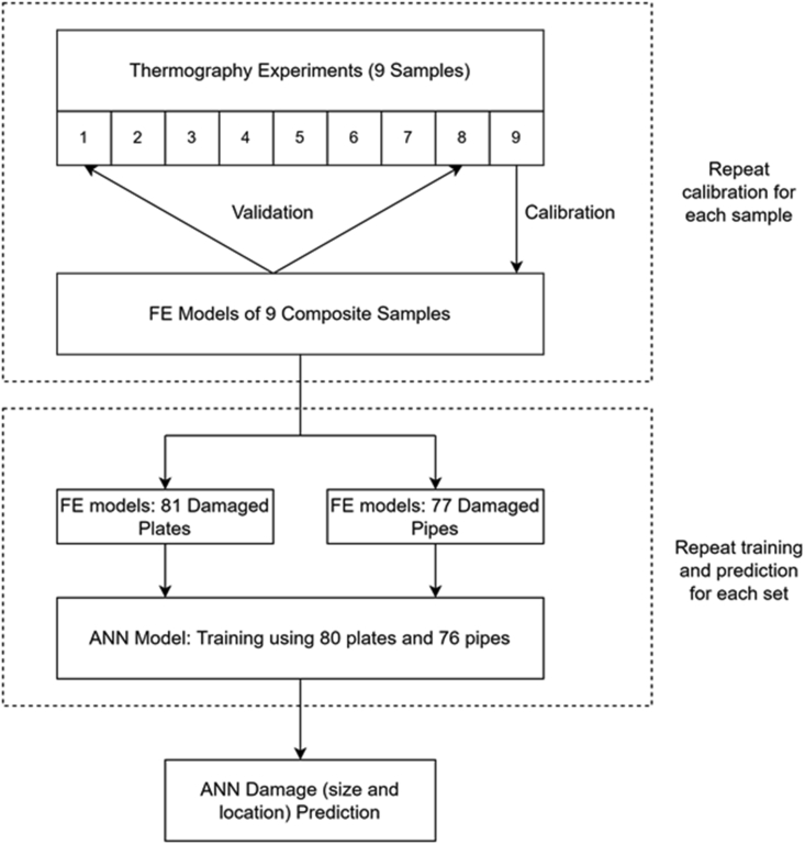
In this work, the thermography readings are used as a benchmark for developing the FE and ANN models. The development of the FE model is divided into three stages: create the FE model, calibrate using one set of data points (sample 9 for example), and validate against the remaining samples (samples 1–8). The calibration is repeated for different sets and validated using the same procedure. The calibrated heat flux and film coefficient values are then fixed for the remaining simulations. The repetition of the calibration is to ensure that the FE model results in the same behavior regardless of the data points used for the calibration. The validated FE model is then extended to create hypothetical models with embedded defects for plates and pipes. This extension is justified through comparing simulation results of plates and pipes with embedded defects of identical size and shape. This comparison study shows the effect of specimen curvature on thermography simulation results. The hypothetical models are a flat plate with a circular shaped embedded defect and a pipe with a rectangular shaped embedded defect. Parametric studies on the hypothetical models are carried out to analyze the effect of each parameter on output results of temperature and thermal images. The relationship between output results and input parameters is further analyzed through ANN models. Figure 1 shows a flowchart summarizing the methodology followed in this work.
Figure 1.
Flowchart of methodology used in the hybrid thermography, computational, ANN damage prediction model.
The main type of defect investigated in this study is debonding, which may be modeled as an embedded defect that is in a plane parallel to the pipe surface. For this reason, the thicknesses used in this study are 1, 2, and 3 layers. Thus, a defect that is aligned in the transverse direction is not applicable for this study, but the approach can be modified to include such damages.
2. Thermography experiments
2.1. Sample preparations
Lock in thermography experiments were carried out on nine composite samples made of unidirectional E glass and epoxy resin as the fiber and reinforcement, respectively, with controlled damage in the form of drilled holes. The plates were custom manufactured and the raw materials were purchased from Hatcon Composite System for wet lay-ups applications. The epoxy types used were LR385 and LR386 with hardeners LH385 and LH386.
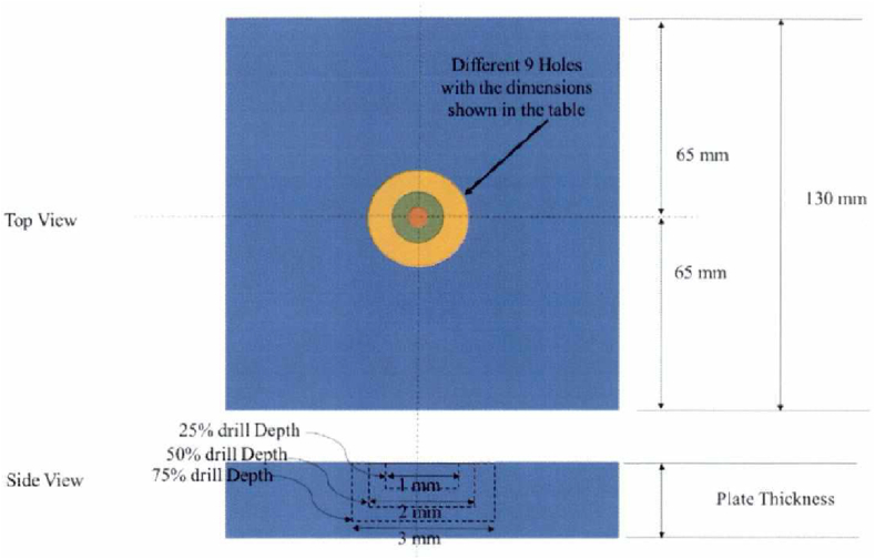
The glass fiber used was BMS9-3-7781 type H3 class 7. The nine samples were manufactured using 20 layers of 1000 mm × 1000mm sheets with a [0°/90°] ply orientation. The sheets were then cut into smaller sheets of 90 mm × 90 mm. The fiber weight was 59.63 g with an epoxy content of 50% per weight. The defects were produced using computer numerical control (CNC) machine-drilled holes of various sizes (1, 2, and 3 mm) at various depths (25%, 50%, and 75%) of plate thickness. A schematic diagram of the composite plates showing all variations in hole size and diameter is shown in Figure 2. Table 1 lists index numbers and dimensions for the nine samples.
Figure 2.
Schematic diagram of composite plates and holes dimensions.
Table 1.
Indexing and dimensions for the nine composite samples.
| Sample No. | Thickness (mm) | Drill Dia. (mm) | Drill Depth (%) | Drill Depth (mm) | Layer Thickness (mm) |
|---|---|---|---|---|---|
| 1 | 5.19 | 1 | 0.25 | 1.3 | 0.260 |
| 2 | 5.28 | 2 | 0.25 | 1.32 | 0.264 |
| 3 | 5.32 | 3 | 0.25 | 1.33 | 0.266 |
| 4 | 5.3 | 1 | 0.5 | 2.65 | 0.265 |
| 5 | 5.25 | 2 | 0.5 | 2.63 | 0.263 |
| 6 | 5.28 | 3 | 0.5 | 2.64 | 0.264 |
| 7 | 5.24 | 1 | 0.75 | 3.93 | 0.262 |
| 8 | 5.3 | 2 | 0.75 | 3.98 | 0.265 |
| 9 | 5.35 | 3 | 0.75 | 4.01 | 0.268 |
2.2. Experimental setup
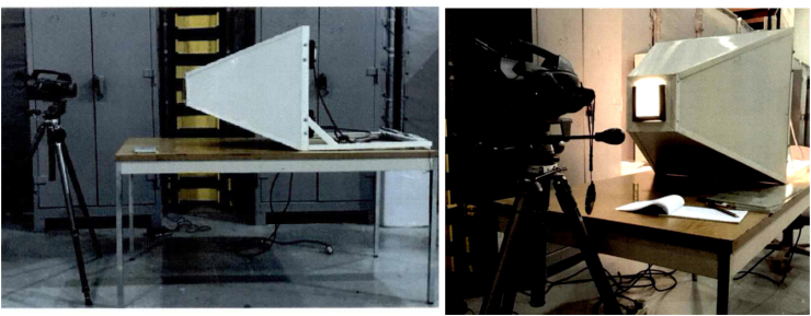
The experimental setup of the lock in thermography is shown in Figure 3. Composite plates were heated using four halogen lamps rated at 500 W each in a contained aluminum hood. The lamps contained within the aluminum hood help in focusing the energy on the composite plate. The experiments were carried out in transmission mode where the non-defected side of the composite sample is heated (from the back of the hood as shown in Figure 3), while the infrared camera takes the readings of the defected side from the front as shown in Figure 3. FLIR GF320 thermal camera was used in this setup. The camera has a spectral range of 4–8 μm, a resolution of 240 × 320 pixels, and a thermal sensitivity of 50mK. This camera has an accuracy of ±1 °C for the temperature range between 0 °C and 100 °C and ±2% for temperatures greater than 100 °C. The optical axis of the camera was perpendicular to the surface of the tested composite plate. The lock-in thermography tests were done for 20 min for each case.
Figure 3.
Side and front view of the thermal imaging experimental setup.
2.3. Thermography results
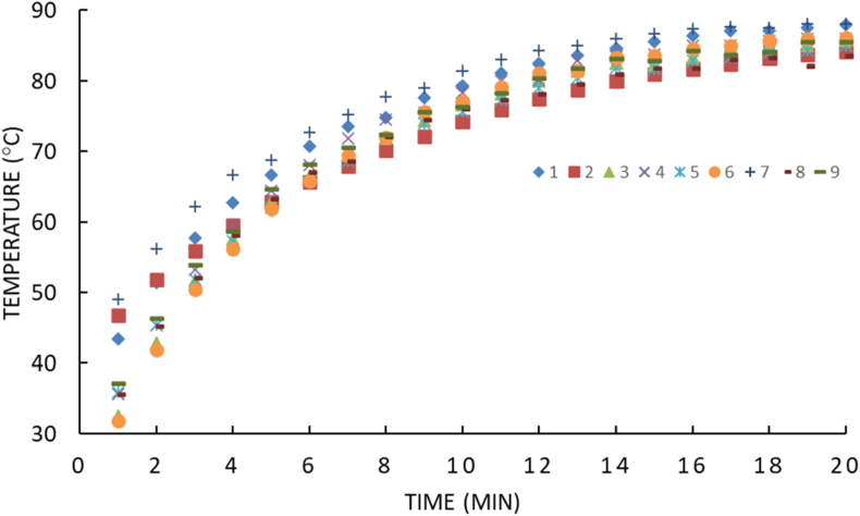
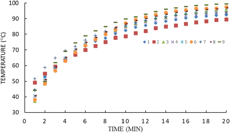
The main goal of the experiments is to correlate between the damage size and temperature profiles. A maximum and minimum temperature measurement is taken at 1 min time intervals for a period of 20 min. The maximum temperature location is found to be at center of the defect while the minimum temperature is found to be in sound regions around the defect. Minimum and maximum temperatures versus time profiles are shown in Figures 4 and 5, respectively.
Figure 4.
Minimum temperature at 1 min intervals.
Figure 5.
Maximum temperature at 1 min intervals.
In the experiments, heat flows through the non-defected side until it reaches a defect. The defect acts as a thermal resistor that impedes heat flow, and this causes temperature to be greater at defect regions compared with sound regions. Therefore, it is expected that temperatures increase with increasing defect size, which is observed in these experiments validating the integrity of the experimental setup and approach.
3. Computational model
The FE model of the composite plates was developed using ANSYS to simulate the experiments carried out on the nine 20 layer composite samples. The objective is to validate the model against the maximum and minimum temperatures since these are available at 1 min intervals and can be extracted from the FE model. In this analysis, sample 9, the plate with 3 mm hole diameter and 75% plate thickness depth, is used for calibration. In calibration, material properties are defined based on the range of values reported in the literature, while boundary conditions and loads are defined based on the thermography experiments. The heat flux and film coefficient were varied in order to obtain optimum experimental data match for temperatures at 1 min intervals for sample 9. Once the model is calibrated by varying heat flux and film coefficient values, the model is validated against samples 6 and 8, which have different hole diameter but same depth, and the same hole diameter but different depth as sample 9, respectively. The procedure is then repeated for the sample 1 to ensure the heat flux and film coefficient values are within the same range of values. The FE model developed in ANSYS used elements SOLID278 and SURF152, which are 8 noded brick and 3D thermal elements, respectively, for the analysis.
3.1. Material properties
Material properties that are required for solving the 3D FE transient heat transfer problem are specific heat, density, and orthotropic thermal conductivity. The density is calculated based on epoxy making up to 50% of composite weight. Table 2 lists the material properties used in this work. The densities of unidirectional Epoxy E-Glass and resin are averaged to be 1595 kg/m3. In-plane and through thickness thermal conductivities are typical for composites where the thermal conductivity is greater in the in-plane directions than through the thickness. These values are close to values used for in-plane and through thickness thermal conductivities and specific heat reported in the literature [16].
Table 2.
Material properties of epoxy E-Glass and resin.
| E-Glass Epoxy Density | 2000 kg/m3 |
|---|---|
| Resin Density | 1.19 g/cm3 |
| In-plane Thermal Conductivity | 5 W/m°C |
| Through-thickness Thermal Conductivity | 0.5 W/m°C |
| Specific heat | 800 J/kgoC |
3.2. FE discretization and BCs
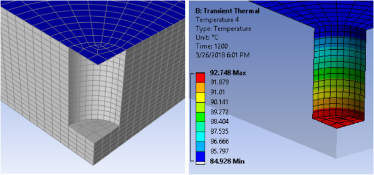
Simulating the lock-in thermography experiment on composite plates requires a transient heat transfer model in 3D as the effect of hole depth on planar temperature is studied. Due to symmetry, only a quarter plate is modeled with uniform heating conditions. Furthermore, ply layup is [0/90°] which makes test specimens symmetric at fiber level. SOLID278 are used for all the elements except for the surface of the plate, where the heat flux is applied, SURF152 elements are used. Figure 6 shows the FE model of the plate quarter model, along with the temperature profile of the defected surface for the simulation of sample 9.
Figure 6.
20-layers composite plate FE model (left) with temperature profile of defected surface (right).
The plate is initially at room temperature; thus, all nodes are set to 22 °C. The applied load is defined by applying a heat flux to the sound side of composite. The defected side has a natural convection with a defined film coefficient and a bulk temperature of 22 °C.
3.3. Model calibration and validation
ANSYS Workbench parametric design study was used to vary heat flux and film convection coefficient and observe the effects on minimum and maximum temperatures. Two random design points were chosen for the calibration to make sure the calibrated values are indifferent to the reference point. DP1 is based on sample 9, while DP2 is based on Sample 1 but with different calibrated values. Table 3 lists the calibrated values of the heat flux, the film coefficient, and the resulting temperature difference compared with the experimental data.
Table 3.
Summary of calibrated values for max. and min temperature at 20 min.
| Design Point | Heat Flux W/mˆ2 | Film Coefficient W/mˆ2 °C | Computational Temp (°C) | Experimental Temp (°C) | Percent Difference Max Temp | Sample |
|---|---|---|---|---|---|---|
| DP1 | 1750 | 27.5 | Max. 97.461 | 99.60 | 2.15 | 9 |
| Min. 83.308 | 85.50 | 2.56 | ||||
| DP2 | 1750 | 26 | Max. 92.377 | 92.40 | 0.02 | 1 |
| Min. 87.528 | 87.90 | 0.42 |
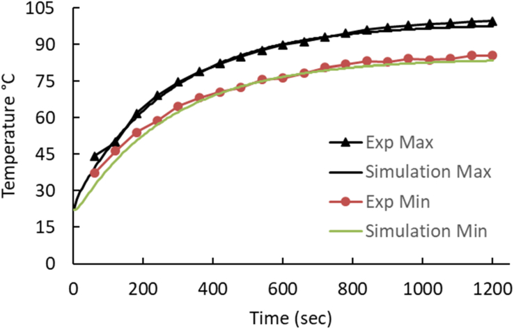
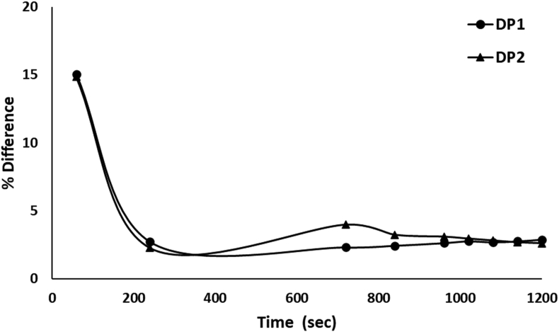
Figure 7 compares the simulated maximum and minimum temperatures with the experimental data at 1 min intervals for DP1. This high level of accuracy between computational and experimental results gives confidence in the heat flux and film coefficient combination. Calibrating the heat flux and film coefficient for different cases validates the model and procedure as long as the calibrated values are proven to be indifferent of the plate hole size and depth. In addition, calibration using a different combination resulted in values that are very close. To ensure the validity of the heat flux and film coefficient combination, the same combination is used for the remaining eight samples for each design point. Figure 8 shows the average percent difference between the experimental and simulated maximum temperature values over time. Both combinations in Table 3 give results with reasonable accuracy, with slight edge for DP1. It is important to note that the relatively large error in the first 3 min is due to the load being applied as a heat flux in the simulation where in the experiment the heat is applied through radiation.
Figure 7.
Comparison between experimental and simulated temperatures for DP1.
Figure 8.
Average % difference between the calibrated DPs and the remaining samples.
4. Computational parametric study on a plate and a pipe with various defects
The validated computational model provides an opportunity to create hypothetical models of thermography setups and use their results without the need for experiments. The computational model is used to simulate cases with composite plates and pipes. Then use the data to enrich an artificial neural network (ANN) model that can predict the composite damage in terms of depth and size. The ANN model is supposed to allow the lock-in reflective thermography simulations fully characterize an embedded defect. This mode is more realistic for composite pipes in the field as it is more appropriate to measure the temperature on the pipe surface.
The parametric study is carried out on two sets of models, plates and pipes, where the embedded defect parameters and other geometrical dimensions are varied. Other model variables such as ply thickness (0.2675 mm), ply layup (45o/-45o), heat flux (1750 W/m2), film coefficient (27.5 W/m2 oC) and initial temperature (22 °C) are held constant in order to isolate the effects of damage size to thermography results.
4.1. Plates with circular embedded defects
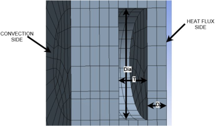
The first set consists of plates with circular shaped embedded defects where the varied parameters are defect diameter “Dia”, defect thickness “T”, defect depth “D”, and plate thickness. Figure 9 shows a section view illustrating these parameters. Table 4 summarizes the parameters varied in the plate parametric study .
Figure 9.
Section view of composite plate with circular shaped embedded defect.
Table 4.
Composite plate parametric study parameters.
| Values | Units | ||||
|---|---|---|---|---|---|
| Defect Diameter | 1 | 2 | 3 | 4 | Mm |
| Defect Thickness | 1 | 2 | 3 | Layers | |||
| Defect Depth | Minimum of 1 layer to a maximum of plate thickness - 2 layers (Top and bottom) | Layers | |||||
| Plate Thickness | 10 | 15 | 20 | Layers | |||
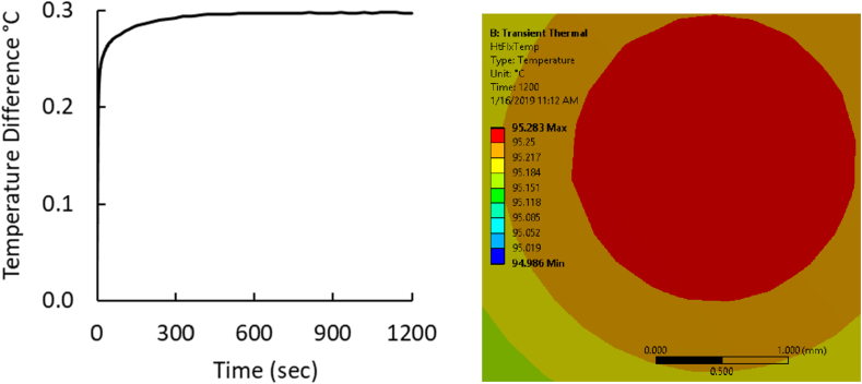
Table 4 lists all possible combinations but not all are simulated, instead only a sample large enough to compare the effects of each parameter on output results is created for this parametric study. A sample size of 81 cases, which includes varying each parameter while holding all others constant, is used. The results generated from the computational simulations are temperature gradients and thermal images. Typical recorded results are shown in Figure 10.
Figure 10.
Sample temperature gradient and steady state thermal image for plate samples.
4.2. Pipes with rectangular embedded defects
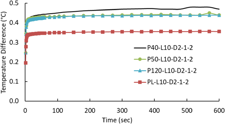
The second set consists of pipes with rectangular shaped embedded defects. First however, it is necessary to justify extending from plates with circular shaped embedded defects to pipes with rectangular shaped embedded defects. This is done by comparing the temperature gradient results of a group of pipes with varying diameter (40, 50, and 120 mm) to a plate where all specimens have an identical embedded defect. The defect is circular shaped with a 2 mm diameter with a single layer for both depth and thickness. The temperature gradients for these pipes are plotted in Figure 11 along with a plate with the same size defect. The temperature gradients converge for pipes of diameter 50 mm and greater for this defect. This indicates that the curvature of the pipe is no longer a factor if the diameter is greater than 50 mm for this case. Furthermore, the converged temperature gradient for the pipe differs from the plate temperature gradient by a small factor. An appropriate multiplication factor may be analyzed as necessary on an as required basis. It is evident that there is a limitation for small diameter pipes as curvature plays a larger role in affecting temperature gradients.
Figure 11.
Temperature gradients for pipes and plate with same size circular defect.
This justifies extending from experimental and computational models that successfully simulate the experimental results of plates to computational models of pipes that are more common in the field. The parameters that are varied in this study are geometrical dimensions of the rectangular shaped embedded defect and the number of composite layers. The geometrical dimensions that fully define a rectangular shaped embedded defect are the two in-plane dimensions (width and length), thickness, and depth. The width represents the distance of the defect in the direction of the z axis while the length represents the distance of the defect along the pipe circumference, and these are identified as “W” and “C”, respectively. The depth is designated as the distance from the heat flux side to the start of the defect and marked as “D”, while thickness is marked as “T”. Figure 12 shows a section view of the pipe with geometrical definitions, along with the sides where heat flux and convection are applied. Table 5 summarizes the parameters varied in the pipe parametric study.
Figure 12.
Section view of pipe with rectangular shaped embedded defect.
Table 5.
Composite pipe parametric study parameters.
| Values | Units | ||||
|---|---|---|---|---|---|
| Defect Distance Along Z Axis, Width, “W” | 1 | 2 | 3 | 4 | mm |
| Defect Circumferential Length “C” | 1 | 2 | 3 | mm | |||
| Defect Thickness “T” | 1 | 2 | 3 | Layers | |||
| Defect Depth “D” | Minimum of 1 layer to a maximum of (plate thickness - 2 layers). Each integer layer depth between minimum and maximum. | Layers | |||||
| Outer Diameter | 40 | 30 | mm | ||||
| Pipe Thickness | 10 | Layers | |||||
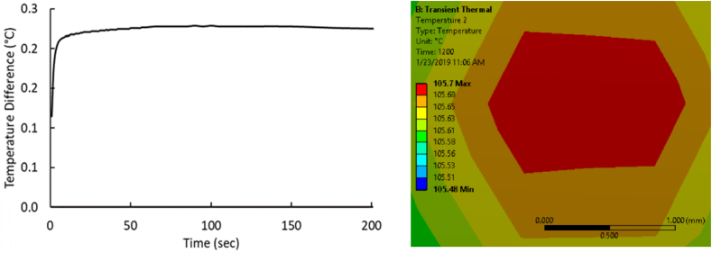
As was done for the plate cases, a sufficient sample size, 77 in this case, was chosen so that it is large enough to include the effects of varying each parameter while holding the rest constant. The temperature gradients and thermal images are obtained from each simulation. Figure 13 shows a typical set of results for a pipe.
Figure 13.
Sample temperature gradient and steady state thermal image for pipe samples.
5. Defects prediction ANN models
The data in this study consists of three parameters, which are temperature gradients, dimensions of red regions in the steady state thermogram, and defect thickness. The temperature gradients and steady state thermogram are generated by the computational FE models for the flat plate and pipe. The temperature gradient is the difference between maximum and minimum temperatures of the side available for inspection, which is the front side for the flat plate and the outer diameter for the pipe. The red region of the steady state thermal image indicates the area of highest temperature of the same face. This red region takes on a circular shape for the flat plate and multiple shapes such as circles, diamonds, and other polygons for the pipe. Dimensions of these red regions are measured using MATLAB image processing to make up the second parameter of the data collection process. The third and final parameter of data collection in this study is the defect thickness. The defect thickness is assumed to be known. This is a realistic scenario as the inspector carrying out thermography can search for a defect thickness of a specific value while carrying out thermography inspection.
The neural networks are created and configured using MATLAB Neural Network Toolkit through the “fitnet” command call. The two arguments of the “fitnet” function are number of hidden layers and training function. The optimum number of hidden layers, representing the number of neurons between the input and output, is set as 10 as it gives accurate results while keeping computation running times practical. A training function based on the Levenberg-Marquardt optim-ization is used in this study to update weight and bias states. The neural networks are trained by accepting the inputs listed in Table 6. The first three arguments to the train function are specified, while the remaining are left as default. The first argument is the network created in this work. The second and third arguments, which are network inputs and network targets, are the results from the computational FE models. The output of the train function is a new network and a training record.
Table 6.
ANN training network inputs.
| Input | Description |
|---|---|
| net | Network |
| X | Network inputs |
| T | Network targets (default = zeros) |
| Xi | Initial input delay conditions (default = zeros) |
| Ai | Initial layer delay conditions (default = zeros) |
| EW | Error weights |
The input to a neural network is an M x N matrix where M is the number of known or measurable values per sample while N is the number of samples. M is composed of outputs from the computational simulations of lock-in thermography and geometric data that is known to the inspector. The computational simulation outputs are temperature gradients at specified time intervals and measurements made on the red region of the steady state thermal image. The geometric data that is known to the inspector and would be able to be measured and selected as a minimum. This geometrical data is the number of composite layers and defect thickness for the plates and pipe in addition to the outer diameter for the pipe. The temperature gradient or the difference between minimum and maximum temperatures of the measured side are obtained at 100 different time intervals. These time intervals are every second for the first minute, every 15 s for the second minute, and every 30 s for the remaining minutes up to 20 min. Thus, there are 60 values from the first minute, 4 values from the first to the second minute, and 36 values for the remaining amount of time up to 20 min. These sum up to 100 temperature gradient measurements.
The dimensions of the red region differ between the flat plate and the pipe, where the red region is a circular shape for the flat plate but takes on multiple shapes for the pipe. For the case of the plate one dimension defines the circle which is the diameter. For the case of the pipe, three parameters are used which are horizontal and vertical dimensions of the red region, and shape type. The number of composite layers is known by the inspector and would be mentioned in documentation of component being inspected. The defect thickness, which is assumed to be a known value in this study, is also treated as an input.
Thus, the value for M in this study is 103 for the plate. This is composed of 100 temperature gradients, the defect thickness, the diameter of the red circle, and the total number of plate layers. On the other hand, the value for M is 105 for the pipe. This is composed of 100 temperature gradients, the defect thickness, and the three parameters obtained from the red region of the steady state thermogram. As mentioned previously, a neural network is created for each sample using the remaining samples to train the network. Therefore, the value for N is the total number of samples minus one. A total of 81 plate samples and 77 pipe samples with varying embedded defect size were simulated.
The network targets are the known outputs that are used to train neural networks. In this study the network targets are the defect details of all samples except the one being tested as they are assumed to be known. The network targets are divided into training, testing, and validation sets with ratios 0.7, 0.15, and 0.15, respectively. The targets are fed to the train function in matrix form. This matrix is P x N size where P is the number of outputs predicted per sample and N is the number of samples. The value for P differs between the flat plate and pipe, where P is 2 for the flat plate and 3 for the pipe. The three dimensions that define the circular shaped embedded defect within the flat plates are defect thickness, defect depth, and defect diameter, indicated as T, D, and Dia in Figure 9. Since defect thickness is taken as a known value, the two target dimensions for the neural network for the plates are defect depth and defect diameter. For the pipe, four dimensions define the rectangular shaped embedded defect. These are defect thickness, defect length along z axis, defect length along pipe circumference, and defect depth. These dimensions are marked as T, W, C, and D in Figure 12.
5.1. ANN for plates with circular shaped embedded defect
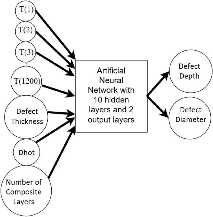
Figure 14 shows inputs and outputs of the ANN for predicting defect depth and defect diameter for the flat plates with circular shaped embedded defects. It is noted that the inputs, which are temperature gradients at selected time intervals, defect thickness, diameter of red circle in steady state thermal image (Dhot), and number of composite layers, are known. The defect depth and defect diameter outputs are unknown.
Figure 14.
ANN for predicting defect depth and defect diameter in flat plates.
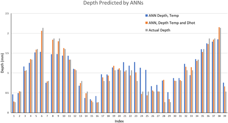
The neural networks are trained to characterize defect size and shape using output data from the thermography simulations. The predicted parameters for the flat plates with circular shaped embedded defects are defect diameter and defect depth. A total of ten neural networks were created for each sample using data from the remaining samples as training data, and the average of the ten neural network predictions was taken. These predicted values were then compared to the actual values from the computational models. Two sets of neural networks were created for the sake of gauging the increased benefit of using thermal image data as feed training data into the ANN. One set uses only temperature gradient data while the second set uses temperature and thermal image data. The prediction results of the ANN models for depth and diameter are shown in Figures 15 and 16. The neural networks that were trained with temperature and Dhot data are much more accurate than neural networks that were trained with only temperature data. Almost all the samples had a very accurate prediction of the depth of the defect.
Figure 15.
Bar Charts of predicted depths and actual depths for flat plates indices 1–39.
Figure 16.
Bar Charts of predicted depths and actual depths for flat plates indices 40–81.
5.2. ANN for pipes with rectangular shaped embedded defect
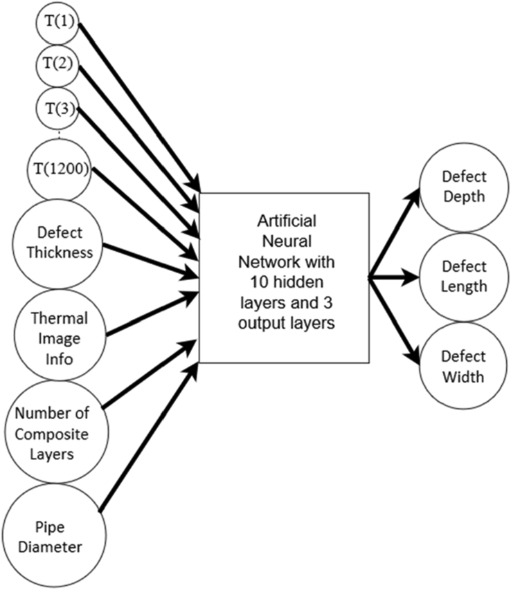
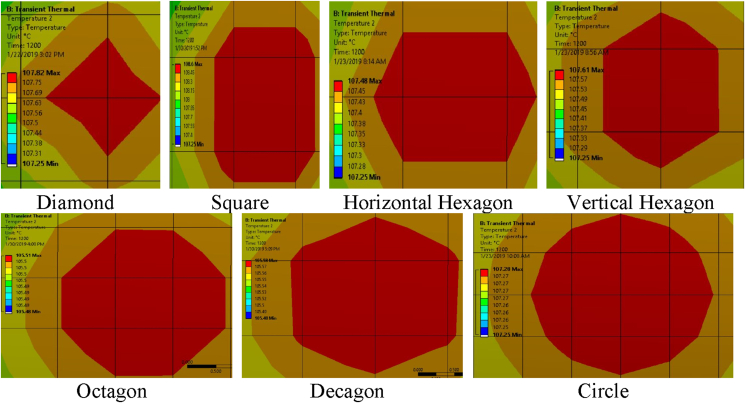
Figure 17 shows the ANN for predicting defect details of the rectangular shaped embedded defect within a pipe. The inputs in this case are temperature gradients at selected time intervals, defect thickness, thermal image information, number of composite layers, and pipe diameter. The thermal images of the pipes are not as uniform as they were for the plates, thus information from these images is quantified and fed into the ANN model. These thermal images are quantified by classifying them based on the hot region shape as shown in Figure 18.
Figure 17.
ANN for predicting defect in plane dimensions and depth in pipes.
Figure 18.
Shape classification for steady state thermal image of pipes.
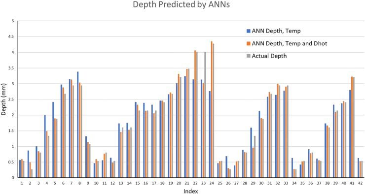
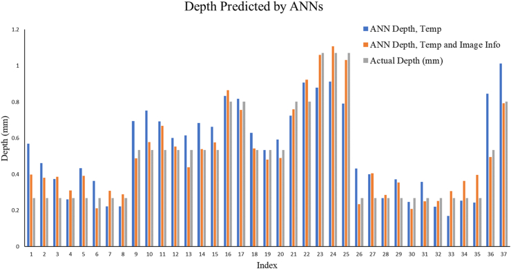
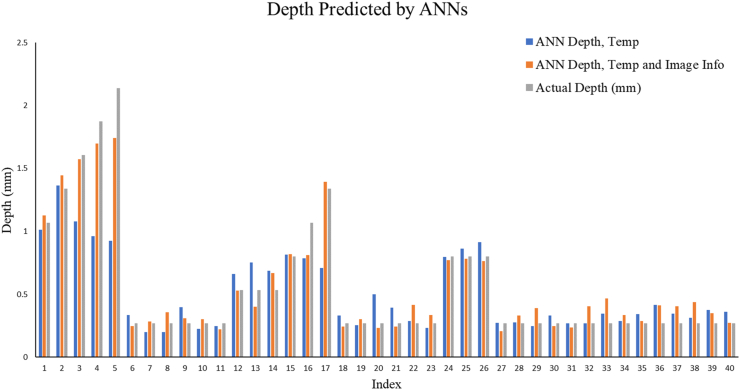
The predicted parameters for the pipes with rectangular shaped embedded defects are defect depth, defect length along z axis, and defect length along circumferential axis. Neural networks were created for each sample using data from the remaining samples as training data, and the average of neural network predictions was taken. These predicted values were then compared to the actual values of the computational model. Figure 19 and Figure 20 show the defect depth prediction results from the ANN model. As in the case of plates, the neural networks that were trained with temperature gradients and thermal image information were more accurate than neural networks that were trained only with temperature gradients.
Figure 19.
Bar Charts of predicted depths and actual depths for pipes indices 1–37.
Figure 20.
Bar Charts of predicted depths and actual depths for pipes indices 38–77.
5.3. ANN results and discussion
The ANN model proved to be highly accurate for predicting defect depths and defect diameters for flat plates with circular shaped embedded defects. Table 7 summarizes the average percent difference for both defect depth and defect diameter for all 81 samples. The results show that even if only the temperature gradient is considered, the average error in depth and diameter would give reasonable results in many cases. Using both temperature gradient and Dhot increases the accuracy tremendously for both defect depth as diameter.
Table 7.
Average % difference for defect depth and diameter of all 81 plate samples.
| Parameter | Neural Network Inputs | Average Percent Difference (%) |
|---|---|---|
| Defect Depth | Temperature and Dhot | 9.5 |
| Defect Depth | Temperature | 27.6 |
| Defect Diameter | Temperature and Dhot | 4.4 |
| Defect Diameter | Temperature | 9.3 |
The neural networks for predicting dimensions of the rectangular shaped embedded defect within the pipes are not as accurate those predicting dimensions of circular shaped embedded defects within flat plates. This is probably due to the added complexity of geometry and extra parameters. Table 8 summarizes the average percent difference for defect depth, defect length, and defect width for all 77 samples.
Table 8.
Average % difference for defect depth, width, and length of all 77 pipe samples.
| Parameter | Neural Network Inputs | Average Percent Difference (%) |
|---|---|---|
| Defect Depth | Temperature and Thermal Image Information | 18.7 |
| Defect Depth | Temperature | 25.3 |
| Defect Width | Temperature and Thermal Image Information | 24.1 |
| Defect Width | Temperature | 29.6 |
| Defect Length | Temperature and Thermal Image Information | 24.8 |
| Defect Length | Temperature | 29.6 |
There are several important implications from this study’s accurate results. First, the thermal image provides more useful information than just qualitative data regarding defects underneath the surface. The thermal image information may be quantified using image processing techniques to create quantitative data. This image data and temperature gradient values may then be fed to an ANN model to train it to predict embedded defect details. As shown in this study, this image data greatly improves the accuracy of ANN predictions from 27.6% to 9.5% difference for predicting defect depth and from 9.3% to 4.4% for predicting defect diameter. Furthermore, these results prove that lock-in thermography may be used with a high level of confidence to predict and characterize embedded defects within composites. It is true that this setup is idealized where the geometry is a flat plate and the embedded defect is perfectly round. However, these results show that this approach involving experimental results of lock-in thermography, computational models simulating the experiments, and training ANNs with data from the computational models to characterize defects is highly effective. This same proven approach may be extrapolated to include different geometries and diff-erent embedded defect shapes with confidence.
The ANNs did not characterize the embedded defects within the pipes as accurately as they did for the embedded defects within the plates. However, the majority overestimate the damage, which is a good from safety point of view. Further, the accuracy of the ANN results for the pipes is improved by quantifying image information and using it to train the neural networks. This improvement in accuracy also occurred in the ANN predictions for the embedded defects within the plates. This proves that the thermal images hold important information that may be used with great success. This information must be quantified using image processing techniques in order to truly gain its benefits. These results make a strong case for thermography as a reliable inspection method for composite pipes in the field. Finally, it is of importance to note that the experimental data was for a flat plate. If experimental data of pipes were used to calibrate the model, it would lead to much more accurate ANN predictions for the composite pipes with embedded defects.
6. Conclusion
This work presented an ANN model based on thermography-based FE models to detect the damage details (geometry, size, etc.) in composite materials. The FE model was validated against experimental thermograms, before being used to develop data of hypothetically embedded defects in composite plates and pipes used to train an ANN model. The results from the ANN model show a high level of accuracy for the plates when using the temperature and diameter of the hot zone, resulting in 4.5 and 9.5 error in the damage diameter and depth, respectively. The ANN model gave acceptable level of accuracy for the pipes, considering the model was calibrated based on a flat plate experimental data, with errors of 18.7, 24.1, and 24.8 in the damage depth, width, and length, respec-tively.
The shape of the embedded defect in plates have a more ideal shape than the in the case of pipes where the embedded defect is circular rather than rectangular. This results in a more uniform heat flow phenomenon in the plate samples compared with the pipes. This greater uniformity in heat flow is directly reflected in the thermography simulation results such as temperature gradient plots versus time and steady state thermal images. For example, the steady state thermal images for the plates show circles of varying diameter, while the steady state thermal images for the pipes show several image types that are classified into seven categories. Thus, it is easy to devise a quantifying value to distinguish between the steady state thermal images of the plates, while it is more difficult to do the same for the pipes.
From an application point of view, ANN coupled with thermal imaging can be used as a live NDT to monitor the health of composite structures. Any industrial operation could develop and validate a simulation model, then develop the ANN model based on the known parameters and properties of the composite pipes used in their operations. For inspection, an engineer or a technician could use live thermal imaging to gather data, which can be inserted directly into the ANN model to predict if there are any hidden defects. This would save time and would provide information that could be used to assess if the defect is at a critical stage in which it needs to be fixed or if it still can withstand operating pressure.
Declarations
Author contribution statement
Khaled S. Al-Athel: Conceived and designed the experiments; Performed the experiments; Analyzed and interpreted the data; Contributed reagents, materials, analysis tools or data; Wrote the paper.
Ahmed S. Alomari: Conceived and designed the experiments; Performed the experiments.
Abul Fazal M. Arif: Conceived and designed the experiments.
Motaz M. Alhasan: Analyzed and interpreted the data; Contributed reagents, materials, analysis tools or data; Wrote the paper.
Funding statement
Khaled Al-Athel was supported by King Fahd University of Petroleum and Minerals.
Data availability statement
Data included in article/supp. material/referenced in article.
Declaration of interest’s statement
The authors declare no conflict of interest.
Additional information
No additional information is available for this paper.
References
- 1.Pastuszak P.D. Characterization of defects in curved composite structures using active infrared thermography. Procedia Eng. 2016;157:325–332. [Google Scholar]
- 2.Al-Athel K.S., Alomari A.S., Arif A.F.M., Alsulaiman F.A., Malik M.H. Damage characterization using thermography of composite plates subjected to low velocity impact loads. J. Mater. Sci. Eng. 2019;8 [Google Scholar]
- 3.Maierhofer C., Myrach P., Reischel M., Steinfurth H., Rollig M., Kunert M. Characterizing damage in CFRP structures using flash thermography in reflection and transmission configurations. Compos. B Eng. 2014;57:35–46. [Google Scholar]
- 4.Ekanayake S., Gurram S., Schmitt R.H. Depth determination of defects in CFRP-structures using lock-in thermography. Compos. B Eng. 2018;147:128–134. [Google Scholar]
- 5.Ghadermazi K., Khozeimeh M.A., Taheri-Behrooz F., Safizadeh M.S. Delamination detection in glass-epoxy composites using step-phase thermography (SPT) Infrared Phys. Technol. 2015;72:204–209. [Google Scholar]
- 6.Alomari A.S., Al-Athel K.S., Arif A.F.M., Al-Sulaiman F.A. Experimental and computational analysis of low-velocity impact on carbon-, glass-and mixed-fiber composite plates. J. Comp. Sci. 2020;4 [Google Scholar]
- 7.Saeed N., Omar M.A., Abdulrahman Y. A neural network approach for quantifying defects depth, for nondestructive testing thermograms. Infrared Phys. Technol. 2018;94:55–64. [Google Scholar]
- 8.Jiayun Chen, Lei Wan, Yaser Ismail, Jianqiao Ye, Dongmin Yang, A micromechanics and machine learning coupled approach for failure prediction of unidirectional CFRP composites under triaxial loading: a preliminary study, Compos. Struct., Volume 267, 2021.
- 9.Gong Jinlong, Liu Junyan, Yu Yanting, Zheng Yi. Multi-characteristic combination based reliability enhancement of optical bidirectional thermal wave radar imaging for GFRP laminates with subsurface defects. NDT E Int. 2021;119 102415. [Google Scholar]
- 10.Gong Jinlong, Zheng Yi, Liu Junyan. A study on the SNR performance analysis of laser-generated bidirectional thermal wave radar imaging inspection for hybrid C/GFRP laminate defects. Infrared Phys. Technol. 2020;111 103526. [Google Scholar]
- 11.Wang Zijun, Wan Litao, Xiong Nanfei, Zhu Junzhen, Ciampa Francesco. Variational level set and fuzzy clustering for enhanced thermal image segmentation and damage assessment. NDT E Int. 2021;118 102396. [Google Scholar]
- 12.Puthiyaveettil Nithin, Rajagopal Prabhu, Krishnan Balasubramaniam. Influence of absorptivity of the material surface in crack detection using laser spot thermography. NDT E Int. 2021;120(102438) ISSN 0963-8695. [Google Scholar]
- 13.Liu K., Ma Z., Liu Y., Yang J., Yao Y. Enhanced defect detection in carbon fiber reinforced polymer composites via generative kernel principal component thermography. Polymers. 2021;13:825. doi: 10.3390/polym13050825. [DOI] [PMC free article] [PubMed] [Google Scholar]
- 14.Liu K., Li Y., Yang J., Liu Y., Yao Y. Generative principal component thermography for enhanced defect detection and analysis. IEEE Trans. Instrum. Meas. 2020;69(10):8261–8269, Oct. [Google Scholar]
- 15.Khan A., Raouf I., Rim Noh Y., Lee D., Woo Sohn J., Soo Kim H. Composite Structures; 2022. Autonomous Assessment of Delamination in Laminated Composites Using Deep Learning and Data Augmentation. [Google Scholar]
- 16.Jinlong G. Infrared Physics & Technology; 2015. Inverse Heat Transfer Approach for Nondestructive Estimation the Size and Depth of Subsurface Defects of CFRP Composite Using Lock-In Thermography; pp. 439–447. [Google Scholar]
Associated Data
This section collects any data citations, data availability statements, or supplementary materials included in this article.
Data Availability Statement
Data included in article/supp. material/referenced in article.


