Ab-initio contrast estimation and denoising of cryo-EM images

Abstract

Background and Objective:

The contrast of cryo-EM images varies from one to another, primarily due to the uneven thickness of the ice layer. This contrast variation can affect the quality of 2-D class averaging, 3-D ab-initio modeling, and 3-D heterogeneity analysis. Contrast estimation is currently performed during 3-D iterative refinement. As a result, the estimates are not available at the earlier computational stages of class averaging and ab-initio modeling. This paper aims to solve the contrast estimation problem directly from the picked particle images in the ab-initio stage, without estimating the 3-D volume, image rotations, or class averages.

Methods:

The key observation underlying our analysis is that the 2-D covariance matrix of the raw images is related to the covariance of the underlying clean images, the noise variance, and the contrast variability between images. We show that the contrast variability can be derived from the 2-D covariance matrix and we apply the existing Covariance Wiener Filtering (CWF) framework to estimate it. We also demonstrate a modification of CWF to estimate the contrast of individual images.

Results:

Our method improves the contrast estimation by a large margin, compared to the previous CWF method. Its estimation accuracy is often comparable to that of an oracle that knows the ground truth covariance of the clean images. The more accurate contrast estimation also improves the quality of image restoration as demonstrated in both synthetic and experimental datasets.

Conclusions:

This paper proposes an effective method for contrast estimation directly from noisy images without using any 3-D volume information. It enables contrast correction in the earlier stage of single particle analysis, and may improve the accuracy of downstream processing.

1. Introduction

In the past decade, single particle reconstruction (SPR) by cryo-electron microscopy (cryo-EM) has emerged as a critical technique for high resolution 3-D structure determination of macromolecules [1,6,10,26,29,30]. In SPR, the 3-D structure needs to be determined from many noisy tomographic projection images with unknown viewing directions. Cryo-EM images are typically very noisy due to the limited electron dosage required to avoid significant radiation damage.

Mathematically, the formation of cryo-EM images can be summarized as follows. Let ϕ(r) be the electrostatic potential of a molecule where $\mathit{r}=(x,y,z{)}^T\in {\mathbb{R}}^3$. The ith observed raw image I_i is modeled as

$${\mathit{I}}_i(x,y)=c_i{\mathit{h}}_i\ast \int \varphi ({\mathit{R}}_i^{-1}\mathit{r})dz+{\mathit{N}}_i.$$ (1)

Namely, the molecule ϕ is first rotated by the rotation matrix R_i, and followed by projection in the z-direction to form the 2-D clean projection image. Next, the clean image is convolved with the 2-D filter h_i, often known as the point spread function, or the inverse Fourier transform of the contrast transfer function (CTF). The convolved ith clean image is further rescaled by its amplitude contrast c_i. At last, additive noise N_i is applied to the resulting image (translations are omitted from (1) just for the sake of simplicity of exposition). The goal of SPR is to estimate ϕ from the set of observed noisy images {I_i}_i∈[n], where [n] ≔ {1, 2, … , n}.

The challenges of SPR lie in several different aspects. First, the noise term N_i typically has much larger magnitude than that of the clean signal, making the clean signal hard to distinguish from the noise even by the naked eye. As a result, a large number of particle images (10⁴ − 10⁶) is often required for reconstruction [6]. Second, the rotations {R_i}_i∈[n] are unknown. These additional unknown variables make the estimation of the 3-D volume difficult in the low signal-to-noise-ratio (SNR) regime. The third challenge arises from the CTF. Although the CTF can be estimated from the power spectrum of the micrograph [12,21,23,38], CTF correction is a challenging deconvolution problem. The main reason is that the CTFs are highly oscillatory and have zeros at many frequencies. Those zero-crossings completely remove the information of the images at those frequencies. As a result, accurate CTF correction requires the usage of several images from different defocus groups (namely different CTFs), assuming that those CTFs have non-overlapping zero-crossings [4]. Last but not least, the underlying clean signals may have different scaling c_i. This amplitude variation is mainly due to the unevenness of the ice layers where the molecule samples reside [34]. Thicker ice layers increase inelastic scattering of electrons by ice, hence decreasing elastic scattering by the molecule and effectively weakening the signal, i.e., a smaller scaling coefficient c_i. The large variation of c_i may cause inaccurate image denoising and CTF correction. Moreover, the scale variations may severely affect the similarity measures used to detect images from similar viewing directions for 2-D class averaging [5,40], 3-D heterogeneity analysis, and the identification of common lines for 3-D ab-initio modeling [2]. In particular, as pointed in Table 2 of [2], the uneven image contrast is the most important factor that negatively affects the accuracy of rotation estimation by some common line based approaches. At last, scaling variability must be accounted for 3-D heterogeneity analysis to prevent artificial classes that correspond to contrast variations [17]. In this work, we aim to address the last challenge, contrast estimation, in the ab-initio stage. In other words, we are interested in the direct estimation of c_i without estimating ϕ and R_i. Furthermore, we use the improved contrast estimation to obtain better denoising and CTF correction of the images.

2. Related work

There exist several works that estimate the amplitude contrast using estimated ϕ and R_i’s [24,27]. Specifically, assuming accurately estimated CTFs and given the estimates $\widehat{\varphi }$, ${\widehat{\mathit{R}}}_i$, one can compute the estimated ith CTF-effected clean image ${\widehat{\mathit{I}}}_i≔{\widehat{\mathit{h}}}_i\ast \int \widehat{\varphi }({\widehat{\mathit{R}}}_i^{-1}\mathit{r})dz$ and then c_i can be estimated as $\langle {\mathit{I}}_i,{\widehat{\mathit{I}}}_i\rangle ∕\Vert {\widehat{\mathit{I}}}_i{\Vert }^2$. The estimates of c_i, R_i and ϕ are often iteratively refined using the EM algorithm [25]. Estimating c_i without any knowledge of rotations and 3-D structure is a challenging task. We refer to this task of contrast estimation as ab-initio contrast estimation (ACE). To the best of our knowledge, ACE has not been extensively studied in previous works. The mean pixel value of the CTF-corrected and denoised images can be used to approximate the contrast. However, [4] only uses the estimated contrasts to filter out junk particles (outliers), while the accuracy of contrast estimation itself was not tested. There are other contrast-related techniques. Image normalization [25,31] rescales the images so that the background noise level is approximately the same across the images. However, its normalization factor depends on the noise level, not the amplitude contrast. There are also works on contrast enhancement [20,32,37]. These aim to enhance the brightness of the underlying signal so that it is more distinguishable from the noise. However, they do not directly estimate the amplitude contrast of the clean signal, and in the process they alter the image contrast.

There are also several commonly used ab-initio methods for simultaneous image denoising and CTF correction, such as traditional Wiener filtering (TWF), and covariance Wiener filtering (CWF) [4]. TWF denoises each image using its own information, which suffers from low SNR and zero-crossings in CTF. CWF overcomes these issues by estimating the population covariance of a set of images. However, its denoising performance degrades when the covariance is not accurately estimated. Image restoration can also be done by 2-D class averaging [9,15,24,40]. These methods require pairwise comparison and alignment of images, unlike the preprocessing methods such as [4] and [7]. It is also shown in [7] that an appropriate image preprocessing can significantly improve the results of 2-D class averaging. Deep learning based methods were recently introduced for image denoising and enhancement [3,11,20,33]. Noise2noise [3] requires multiple video frames of the same micrograph, which are not always available. Other CNN and GAN based methods [11,20,33] require clean projections to form clean-noisy pairs of images to train the model, but the clean projections are not available in the ab-initio reconstruction stage, and training with clean projections of other molecules may introduce model bias.

3. Methodology

In this work, we directly estimate the amplitude contrast from the CTF-corrected and denoised images in the ab-initio stage of SPR. Our method is based on CWF with additional constraints on the covariance matrix which we find realistic and useful for contrast estimation.

In order to address the ACE problem, we first derive from (1) a simplified image formation model that is independent of R_i and ϕ. We then propose our method to solve the ACE problem under this model.

3.1. A Simplified Image formation model

To demonstrate the simplified model, we first reshape the images in (1) as vectors and obtain

$${\mathit{y}}_i=c_i{\mathit{A}}_i{\mathit{x}}_i+{ϵ}_i$$ (2)

where y_i and x_i are respectively the vectors of ith noisy and clean images, A_i is the square matrix operator corresponding to the convolution with h_i, ϵ_i is the Gaussian noise vector and c_i is the contrast to be estimated. In this model, c_i, x_i and ϵ_i are unknown. However, the power spectral density (PSD) of ϵ_i is assumed known as it can be estimated from the corners of the observed images y_i. We assume that A_i and its Fourier transform, the CTF, are known, since they can often be accurately estimated in advance from the noisy micrographs. Throughout this work, we assume that the CTFs are radially symmetric by ignoring astigmatism. Without loss of generality (WLOG) we assume that the noise distribution is white Gaussian whose covariance is σ²I. For colored Gaussian noise, one can whiten the noise by applying W (noise covariance to the power −1/2) to y_i, so that Wy_i = c_iWA_ix_i + Wϵ_i and the covariance of the whitened noise Wϵ_i is the identity matrix. The goal of ACE is to estimate c_i from the observed y_i.

Without additional assumptions on x_i and c_i, the ACE problem is ill-posed due to the scale ambiguity of x_i and c_i. To make it a well-posed problem, WLOG we assume that x_i and c_i are random variables such that for all i ∈ [n],

1. c_i and x_i are independent of each other.

2. $\mathbb{E}(c_i)=1$.

3. ${\mathit{x}}_i^{\mathsf{T}}1=s$ for some constant s > 0, where 1 is the all-ones vector of the same size as x_i.

The first assumption is reasonable since the contrast c_i primarily depends on the thickness of the ice layer, which is indeed independent of the rotation R_i and consequently independent of x_i. The second assumption is needed to overcome the global scale ambiguity of c_i. The last assumption states that the sum of pixel values of the clean projection image is the same for all clean images. This is a reasonable assumption, because for each i ∈ [n], the sum of the elements in x_i is approximately $\int \int (\int \varphi ({\mathit{R}}_i^{-1}\mathit{r})dz)dxdy=\int \varphi (\mathit{r})d\mathit{r}$ which is a constant independent of i. In other words, the sum of pixel values of any 2-D projection image equals the sum of 3-D voxel values. In fact, it is also invariant to translations (i.e., non-perfect centering of the images).

We note that our model assumes that c_i’s are identically distributed, but it does not require the contrasts to be independent of each other. Namely, we allow correlations among c_i’s, which is often observed in experimental data. For example, two particle images that are closely located in the same micrograph often share similar contrasts. In principle, this information can be used to improve the contrast estimation, but this is left to future work. We refer the reader to Fig. 23 in Section 5.1 for further discussion.

Fig. 23.

Demonstration of the relationship between the contrast of picked particle and their locations in the micrographs of EMPIAR-10028. Each dot corresponds to a particle image, whose color represents its estimated contrast.

We remark that the estimation of c_i remains challenging due to the CTF that affects the sum of pixel values and due to the high noise level. Thus, in order to obtain a good estimate of c_i, it is useful to denoise the image and to correct the CTF effect. A well-known method for such image restoration is CWF [4], which is elaborated in the next subsection.

3.2. Preliminaries: Covariance wiener filtering

CWF estimates c_ix_i from y_i by minimizing the expected mean squared error given an estimated covariance matrix of c_ix_i. Assume that the true covariance matrix of c_ix_i, denoted by Σ_cx, is given by an oracle. Then, under the model y_i = A_i(c_ix_i) + ϵ_i, the linear minimum mean squared error (LMMSE) estimator is given by

$${\widehat{c_i{\mathit{x}}_i}}^{\text{CWF}}=\text{CWF}({\mathit{y}}_i,{\mathit{A}}_i,{\Sigma }_{cx})=\underset{\widehat{c_i{\mathit{x}}_i}}{\text{arg}\text{min}}\mathbb{E}(\Vert \widehat{c_i{\mathit{x}}_i}-c_i{\mathit{x}}_i{\Vert }^2\mid {\mathit{y}}_i)$$ (3)

$$=\mu +{\Sigma }_{cx}{\mathit{A}}_i^{\mathsf{T}}({\mathit{A}}_i{\Sigma }_{cx}{\mathit{A}}_i^{\mathsf{T}}+{\sigma }^2\mathit{I}{)}^{-1}({\mathit{y}}_i-{\mathit{A}}_i\mu ),$$ (4)

where μ is the true mean of c_ix_i.

We note that CWF naturally induces an optimal linear estimator of contrast given the true covariance Σ_cx. Indeed, it can be easily shown that :

$$\begin{gathered} \underset{1^{\mathsf{T}}\widehat{c_i{\mathit{x}}_i}}{\text{arg}\text{min}}\mathbb{E}(\Vert 1^{\mathsf{T}}\widehat{c_i{\mathit{x}}_i}-1^{\mathsf{T}}{c}_i{\mathit{x}}_i{\Vert }^2\mid {\mathit{y}}_i) \\ =1^{\mathsf{T}}\mu +1^{\mathsf{T}}{\Sigma }_{cx}{\mathit{A}}_i^{\mathsf{T}}({\mathit{A}}_i{\Sigma }_{cx}{\mathit{A}}_i^{\mathsf{T}}+{\sigma }^2\mathit{I}{)}^{-1}({\mathit{y}}_i-{\mathit{A}}_i\mu )=1^{\mathsf{T}}{\widehat{c_i{\mathit{x}}_i}}^{\text{CWF}}. \end{gathered}$$ (5)

Namely, $1^{\mathsf{T}}{\widehat{c_i{\mathit{x}}_i}}^{\text{CWF}}$, the sum of pixel values of the CWF estimate of c_ix_i, is the best linear estimator of 1^⊤c_ix_i given Σ_cx. Note that 1^⊤c_ix_i = s · c_i by the third assumption of our model. Therefore, we have obtained the optimal linear estimator of contrast c_i up to a global constant s. This scale ambiguity can be solved by using the second assumption $\mathbb{E}(c_i)=1$ in our model. That is, after obtaining the estimates of s · c_i, we normalize the estimates by a global constant so that the average of the set $\{1^{\mathsf{T}}{\widehat{c_i{\mathit{x}}_i}}^{\text{CWF}}{\}}_{i\in [n]}$ is 1.

However, the optimal properties of the aforementioned estimates only hold when Σ_cx is given, which is not true in practice. In [4], the mean of c_ix_i is estimated by minimizing the least squares error between the noisy images and the CTF transformed mean. Specifically,

$$\widehat{\mu }=\underset{\mu }{\text{arg}\text{min}}\sum _{i=1}^n\Vert {\mathit{y}}_i-{\mathit{A}}_i\mu {\Vert }^2.$$ (6)

Similarly, the covariance matrix Σ_cx is estimated by minimizing the squared deviations between the sample covariance of y_i and the population covariance of A_i(c_ix_i) + ϵ_i. That is,

$${\widehat{\Sigma }}_{cx}=\underset{\Sigma }{\text{arg}\text{min}}\sum _{i=1}^n{\Vert ({\mathit{y}}_i-{\mathit{A}}_i\widehat{\mu })({\mathit{y}}_i-{\mathit{A}}_i\widehat{\mu }{)}^{\mathsf{T}}-({\mathit{A}}_i\Sigma {\mathit{A}}_i^{\mathsf{T}}+{\sigma }^2\mathit{I})\Vert }_F^2.$$ (7)

By setting the first order derivative of (7) to zero, we end up with the following linear system of equations:

$$\sum _{i=1}^n{\mathit{A}}_i^{\mathsf{T}}{\mathit{A}}_i{\widehat{\Sigma }}_{cx}{\mathit{A}}_i^{\mathsf{T}}{\mathit{A}}_i=\sum _{i=1}^n{\mathit{A}}_i^{\mathsf{T}}({\mathit{y}}_i-{\mathit{A}}_i\widehat{\mu })({\mathit{y}}_i-{\mathit{A}}_i\widehat{\mu }{)}^{\mathsf{T}}{\mathit{A}}_i+{\sigma }^2\sum _{i=1}^n{\mathit{A}}_i^{\mathsf{T}}{\mathit{A}}_i.$$ (8)

We note that the first term on the right hand side (RHS) of (8) corresponds to the sample covariance of ${\mathit{A}}_i^{\mathsf{T}}{\mathit{y}}_i$. However, y_i often has dimension > 10⁴ which is comparable to the number of images. In this high dimensional setting, the sample covariance is not a consistent estimator of the population covariance. As a result, an eigenvalue shrinkage method is applied to the RHS of (8) to improve the covariance estimation. At last, (8) is solved by applying the conjugate gradient method. We refer the readers to [4] for more details.

We remark that under low SNR or insufficient number of samples, Σ_cx could be poorly estimated. In such a case, the CWF method and its induced contrast estimator (5) are far from being optimal. Therefore, there is still room for improvement on the CWF-based contrast estimation. Indeed, the CWF-estimator does not fully exploit our model assumptions. As we show in the next subsection, the three assumptions of our model imply novel constraints on Σ_cx which turn out to significantly improve contrast estimation.

3.3. Novel constraints on the covariance matrices

The new constraints on the covariance matrix are stated in the following proposition. Let Σ_x be the true covariance of x_i and Var(c) be the variance of each c_i.

Proposition 1.If the three assumptions for themodel (2)are satisfied, then the following two constraints hold:

1. $${\Sigma }_{cx}=(\text{Var}(c)+1){\Sigma }_x+\text{Var}(c)\mu {\mu }^{\mathsf{T}}$$ (9)
2. $${\Sigma }_{x}1=0.$$ (10)

This proposition suggests that the true covariance of c_ix_i is the combination of two components, one corresponds to the covariance without contrast variability whose eigenvectors are perpendicular to the all-ones vector, and the other corresponds to a rank-one matrix whose eigenvector is the mean. The derivation of the two constraints is simple. To prove the first constraint, we use the identity that for any independent scalar random variable c and random vector x, $\text{Cov}(c\mathit{x})=\mathbb{E}(c^2)\text{Cov}(\mathit{x})+\text{Var}(c)\mathbb{E}(\mathit{x})\mathbb{E}(\mathit{x}{)}^{\mathsf{T}}$. By letting c = c_i and x = x_i, we obtain that for any i ∈ [n]

$$\begin{gathered} {\Sigma }_{cx}=\text{Cov}(c\mathit{x})=\mathbb{E}(c^2)\text{Cov}(\mathit{x})+\text{Var}(c)\mathbb{E}(\mathit{x})\mathbb{E}(\mathit{x}{)}^{\mathsf{T}} \\ =(\text{Var}(c)+{\mathbb{E}}^2(c)){\Sigma }_x+\text{Var}(c)\mu {\mu }^{\mathsf{T}}. \end{gathered}$$

By using the assumption $\mathbb{E}(c_i)=1$, we conclude the first constraint. The second constraint states that the variation of the sum of elements in x_i is 0, namely the contrast variability of clean signals is 0. It can be verified easily by using the third assumption of our model. Specifically,

$${\Sigma }_{x}1=\mathbb{E}\left(({\mathit{x}}_i-\mu )({\mathit{x}}_i-\mu {)}^{\mathsf{T}}\right)1=\mathbb{E}\left(({\mathit{x}}_i-\mu )({\mathit{x}}_i^{\mathsf{T}}1-{\mu }^{\mathsf{T}}1)\right)=0,$$

where the last equality follows from the assumption that : ${\mathit{x}}_i^{\mathsf{T}}1={\mu }^{\mathsf{T}}1=s$. In the next subsection, we propose two methods that use the two covariance constraints to refine the estimated covariance Σ_cx.

3.4. Refinement of covariance matrices

We first use the two covariance constraints (9) and (10) to estimate the contrast variance Var(c). By combining the two constraints,

$${\Sigma }_{cx}1=(\text{Var}(c)+1){\Sigma }_{x}1+\text{Var}(c)\mu {\mu }^{\mathsf{T}}1=\text{Var}(c)\mu {\mu }^{\mathsf{T}}1,$$ (11)

where the second equality follows from the second covariance constraint. We note that (11) relates Var(c) to Σ_cx and μ, where the latter two can be estimated from the noisy data. Given the estimated ${\widehat{\Sigma }}_{cx}$ and $\widehat{\mu }$, the variance of the image contrast can be estimated by least squares as follows.

$$\widehat{\text{Var}(c)}=\underset{\text{Var}(c)}{\text{arg}\text{min}}\Vert {\widehat{\Sigma }}_{cx}1-\text{Var}(c)({\widehat{\mu }}^{\mathsf{T}}1)\widehat{\mu }{\Vert }_2^2=\frac{{\widehat{\mu }}^{\mathsf{T}}{\widehat{\Sigma }}_{cx}1}{\Vert \widehat{\mu }{\Vert }^2{\widehat{\mu }}^{\mathsf{T}}1}.$$ (12)

We remark that the initially estimated ${\widehat{\Sigma }}_{cx}$ often does not satisfy the constraints in Proposition 1. Therefore, we introduce two methods to enforce the covariance constraints using the estimated $\widehat{\text{Var}(c)}$. We refer to the first method as semi-definite programming (SDP).

SDP:

We seek to find the closest positive semidefinite matrix to the initially estimated ${\widehat{\Sigma }}_{cx}$ such that the two covariance constraints are satisfied. Namely, we seek a solution of the following SDP problem.

$${\widehat{\Sigma }}_{cx}^{\text{SDP}}=\underset{{\Sigma }_{cx}^{\text{SDP}}}{\text{arg}\text{min}}{\Vert {\Sigma }_{cx}^{\text{SDP}}-{\widehat{\Sigma }}_{cx}\Vert }_F^2$$ (13)

subject to ${\Sigma }_{cx}^{\text{SDP}}=(\widehat{\text{Var}(c)}+1){\Sigma }_x^{\text{SDP}}+\widehat{\text{Var}(c)}\widehat{\mu }{\widehat{\mu }}^{\mathsf{T}}$

$$\begin{gathered} {\Sigma }_{cx}^{\text{SDP}}\underset{¯}{\succ }0 \\ {\Sigma }_x^{\text{SDP}}\underset{¯}{\succ }0 \\ {\Sigma }_x^{\text{SDP}}1=0. \end{gathered}$$

Since ${\Sigma }_{cx}^{\text{SDP}}=(\widehat{\text{Var}(c)}+1){\Sigma }_x^{\text{SDP}}+\widehat{\text{Var}(c)}\widehat{\mu }{\widehat{\mu }}^{\mathsf{T}}$, ${\Sigma }_{cx}^{\text{SDP}}$ is positive semidefinite when ${\Sigma }_x^{\text{SDP}}$ is so. Thus, one can drop the constraint ${\Sigma }_{cx}^{\text{SDP}}\underset{¯}{\succ }0$, and plug in the first constraint of (13) to ${\Sigma }_{cx}^{\text{SDP}}$ in its objective function. This yields the following SDP fomulation that optimizes for ${\Sigma }_x^{\text{SDP}}$.

$${\widehat{\Sigma }}_x^{\text{SDP}}=\underset{{\Sigma }_x^{\text{SDP}}}{\text{arg}\text{min}}{\Vert {\Sigma }_x^{\text{SDP}}-\frac{{\widehat{\Sigma }}_{cx}-\widehat{\text{Var}(c)}\widehat{\mu }{\widehat{\mu }}^{\mathsf{T}}}{\widehat{\text{Var}(c)}+1}\Vert }_F^2$$ (14)

subject to ${\Sigma }_x^{\text{SDP}}1=0$

$${\Sigma }_x^{\text{SDP}}\underset{¯}{\succ }0.$$

After solving ${\widehat{\Sigma }}_x^{\text{SDP}}$, we immediately obtain ${\widehat{\Sigma }}_{cx}^{\text{SDP}}=(\widehat{\text{Var}(c)}+1){\widehat{\Sigma }}_x^{\text{SDP}}+\widehat{\text{Var}(c)}\widehat{\mu }{\widehat{\mu }}^{\mathsf{T}}$. Next, we introduce a faster but heuristic alternative that uses the Gram-Schmidt (GS) process to approximately solve (14).

Gram-Schmidt (GS) Process:

We first note that the constraint ${\Sigma }_x^{\text{SDP}}1=0$ in (14) is equivalent to that all the eigenvectors of ${\Sigma }_x^{\text{SDP}}$ are orthogonal to 1. Similar to (14), we seek a positive semidefinite matrix ${\Sigma }_x^{\text{GS}}$ that is close to ${\widehat{\Sigma }}_x≔({\widehat{\Sigma }}_{cx}-\widehat{\text{Var}(c)}\widehat{\mu }{\widehat{\mu }}^{\mathsf{T}})∕(\widehat{\text{Var}(c)}+1)$ whose eigenvectors are orthogonal to 1.

Let ${\widehat{\Sigma }}_x=\widehat{\mathit{V}}\widehat{\mathit{D}}{\widehat{\mathit{V}}}^{\mathsf{T}}$ be the eigenvalue decomposition of ${\widehat{\Sigma }}_x$, where $\widehat{\mathit{V}}$ is the eigenmatrix whose columns are eigenvectors of ${\widehat{\Sigma }}_x$, and $\widehat{\mathit{D}}$ is the diagonal matrix of its eigenvalues. We seek a refined covariance ${\widehat{\Sigma }}_x^{\text{GS}}=\widehat{\mathit{U}}\widehat{\Lambda }{\widehat{\mathit{U}}}^{\mathsf{T}}$ with refined eigenvalues and eigenvectors such that $\widehat{\Lambda }$ is nonnegative (so that ${\widehat{\Sigma }}_x^{\text{GS}}\underset{¯}{\succ }0$) and ${\widehat{\mathit{U}}}^{\mathsf{T}}1=0$ (so that $({\widehat{\Sigma }}_x^{\text{GS}}{)}^{\mathsf{T}}1=0$), and $\widehat{\Lambda }$ and $\widehat{\mathit{U}}$ are respectively close to $\widehat{\mathit{D}}$ and $\widehat{\mathit{V}}$.

The solution of $\widehat{\Lambda }$ is obtained by simply thresholding the negative values in $\widehat{\mathit{D}}$. That is, $\widehat{\Lambda }=\max (\widehat{\mathit{D}},0)$. The solution of the eigenmatrix $\widehat{\mathit{U}}$ is trickier, due to the nonconvex constraint ${\widehat{\mathit{U}}}^{\mathsf{T}}\widehat{\mathit{U}}=\mathit{I}$, namely the columns of $\widehat{\mathit{U}}$ (the eigenvectors of ${\widehat{\Sigma }}_x^{\text{GS}}$) form an orthonormal basis. It asks to solve the following nonconvex optimization problem.

$$\widehat{\mathit{U}}=\underset{\mathit{U}}{\text{arg}\max }\text{Tr}({\widehat{\mathit{V}}}^{\mathsf{T}}\mathit{U})$$ (15)

subject to U^⊤U = I

$${\mathit{U}}^{\mathsf{T}}1=0.$$

Instead of directly solving (15), we argue that a simple Gram-Schmidt process on $\widehat{\mathit{V}}$ is often sufficient to obtain a satisfying solution. Let $\widehat{\mathit{V}}=[{\widehat{\mathit{v}}}_1,{\widehat{\mathit{v}}}_2,\dots ,{\widehat{\mathit{v}}}_p]$ where p is the dimension of each x_i, and the eigenvectors are placed in descending order of eigenvalues.

Let $\widehat{\mathit{U}}≔[{\widehat{\mathit{u}}}_1,{\widehat{\mathit{u}}}_2,\dots ,{\widehat{\mathit{u}}}_p]$ and $[1,{\widehat{\mathit{V}}}_{-p}]≔[1,{\widehat{\mathit{v}}}_1,{\widehat{\mathit{v}}}_2,\dots ,{\widehat{\mathit{v}}}_{p-1}]$ be p-by-p square matrices. Application of Gram-Schmidt orthogonalization to $[1,{\widehat{\mathit{V}}}_{-p}]$ yields a new orthogonal matrix $[1,{\widehat{\mathit{U}}}_{-p}]≔[1,{\widehat{\mathit{u}}}_1,{\widehat{\mathit{u}}}_2,\dots ,{\widehat{\mathit{u}}}_{p-1}]$. That is, ${\widehat{\mathit{u}}}_1$ is computed by projecting ${\widehat{\mathit{v}}}_1$ onto the orthogonal complement of 1 and then normalize to unit vector. Once ${\widehat{\mathit{u}}}_{i-1}$ for 1 ≤ i ≤ p − 1 are computed, ${\widehat{\mathit{u}}}_i$ is computed by projecting ${\widehat{\mathit{v}}}_i$ onto the orthogonal complement of linear subspace spanned by $1,{\widehat{\mathit{u}}}_1,\dots ,{\widehat{\mathit{u}}}_{i-1}$ and then normalize. At last, the solution $\widehat{\mathit{U}}$ is obtained by finding the orthogonal complement of ${\widehat{\mathit{U}}}_{-p}$ to complete its missing column ${\widehat{\mathit{u}}}_p$. In this way, the columns of $\widehat{\mathit{U}}$ form an orthonormal basis, and its first p − 1 columns are orthogonal to 1. Although ${\widehat{\mathit{u}}}_p$ may not necessarily be orthogonal to 1, its eigenvalue is 0 in most of the cases and thus won’t affect the solution of ${\widehat{\Sigma }}_x^{\text{GS}}$. In practice, the GS process is done by the QR decomposition for its better numerical stability.

Iterating from the top eigenvectors has two benefits. First, the top eigenvectors of ${\widehat{\Sigma }}_x$ are more robust to the noise. That is, the top eigenvectors ${\widehat{\mathit{v}}}_1,{\widehat{\mathit{v}}}_2,\dots$ of ${\widehat{\Sigma }}_x$ are often closer to those of the true Σ_x. Due to the constraint Σ_x1 = 0, the top eigenvectors of ${\widehat{\Sigma }}_x$ often have smaller correlation with 1. In other words, the top eigenvectors are cleaner and thus their refinement is easier and more accurate, and therefore they should be put at the earlier stage of the sequential projection procedure to reduce error accumulation. Second, iterating from the top eigenvectors makes them more accurately projected to the orthogonal complement of 1 with minimal changes to their original values. This is beneficial for contrast estimation since these top eigenvectors are more important for explaining the contrast variations.

3.5. Ab-initio contrast estimation and denoising

After applying the aforementioned SDP or GS method to the initial covariance matrix ${\widehat{\Sigma }}_{cx}$, we obtain the refined covariance ${\widehat{\Sigma }}_{cx}^{\text{RF}}={\widehat{\Sigma }}_{cx}^{\text{SDP}}$ or ${\widehat{\Sigma }}_{cx}^{\text{GS}}$.

Recall that the CWF estimator of c_ix_i is defined in (3). Our refined estimate of c_ix_i for each i ∈ [n] is

$${\widehat{c_i{\mathit{x}}_i}}^{\text{RF}}=\text{CWF}\left({\mathit{y}}_i,{\mathit{A}}_i,{\widehat{\Sigma }}_{cx}^{\text{RF}}\right).$$ (16)

Then, by applying our model assumptions that 1^⊤x_i = s for all i ∈ [n] and $\mathbb{E}(c_i)=1$, we obtain our refined estimate of c_i as

$${\widehat{c_i}}^{\text{RF}}=\frac{1^{\mathsf{T}}{\widehat{c_i{\mathit{x}}_i}}^{\text{RF}}}{\frac{1}{n}{\sum }_{i=1}^n{1}^{\mathsf{T}}{\widehat{c_i{\mathit{x}}_i}}^{\text{RF}}},$$ (17)

where the numerator is the contrast estimator up to s. The denominator is the normalization factor to remove the scale ambiguity and enforce the average of ${\widehat{c_i}}^{\text{RF}}$ to be 1.

After estimating the contrasts, we present two methods for estimating the clean image x_i: the image normalization and 2-stage CWF.

Image Normalization

In the first approach, we estimate x_i as

$${\widehat{\mathit{x}}}_i^{\text{RF}}=\frac{{\widehat{c_i{\mathit{x}}_i}}^{\text{RF}}}{{\widehat{c_i}}^{\text{RF}}}.$$ (18)

That is, we simply normalize the estimated c_ix_i by the estimated contrast c_i, so that the resulting images all share the same sum of pixel values.

2-Stage CWF

In the second method, we apply an additional CWF estimator to directly estimate x_i. Recall that the original version of CWF aims to estimate c_ix_i. It treats c_ix_i as a single variable and considers the model y_i = A_i(c_ix_i) + ϵ_i. In order to directly estimate x_i, we treat c_i as known and absorb it into the CTF term, and consider the model ${\mathit{y}}_i=({\widehat{c_i}}^{\text{RF}}{\mathit{A}}_i){\mathit{x}}_i+{ϵ}_i$. Given this model, a natural estimate of x_i is

$${\widehat{\mathit{x}}}_i^{\text{RF}}=\text{CWF}\left({\mathit{y}}_i,{\widehat{c_i}}^{\text{RF}}{\mathit{A}}_i,{\widehat{\Sigma }}_x^{\text{RF}}\right).$$ (19)

Since the refined ${\widehat{\Sigma }}_x^{\text{RF}}$ satisfies the constraint ${\widehat{\Sigma }}_x^{\text{RF}}1=0$, the resulting recovered image ${\widehat{\mathit{x}}}_i^{\text{RF}}$ automatically has the same sum of pixel values. Ideally, if ${\widehat{c_i}}^{\text{RF}}=c_i$ and ${\widehat{\Sigma }}_x^{\text{RF}}={\Sigma }_x$, then (19) is the optimal linear estimator of x_i.

3.6. Computational issues and steerable basis

Although our model and methodology were presented in real image space for simplicity, in practice, implementing the CWF-based methods in real image domain is computationally intractable and memory demanding. For images of size L × L, the dimension of x_i is of order O(L²), and the covariance of x_i in real space has O(L⁴) entries. This leads to high time and space complexities that make the computation impractical.

Therefore, we follow [4] and expand the Fourier transformed images ℱ(I_i) in the Fourier-Bessel basis

$${\psi }_r^{k,q}(\theta ,\xi )=\{\begin{array}{cc}{N}_{k,q}{J}_k(R_{k,q}\xi ∕r)e^{1k\theta }\hfill & \xi \le r\hfill \\ 0\hfill & \text{otherwise},\hfill \end{array}\phantom{\}}$$ (20)

where 0 < r ≤ 1/2 is the band-limit radius of images (default = 1/2), k, q are respectively angular and radial frequencies, (ξ, θ) are the polar coordinates in Fourier domain, J_k is the Bessel function of the first kind of order k, R_k,q is the qth root of J_k, and $N_{k,q}=(r\sqrt{\pi }\mid J_{k+1}(R_{k,q})\mid {)}^{-1}$ is the normalization factor. We refer the readers to [39] for details of the expansion.

Denote the image formation model in the Fourier-Bessel basis as

$${\mathit{y}}_i^{\text{FB}}=c_i{\mathit{A}}_i^{\text{FB}}{\mathit{x}}_i^{\text{FB}}+{ϵ}_i$$

where ${\mathit{A}}_i^{\text{FB}}$, ${\mathit{x}}_i^{\text{FB}}$ ${\mathit{y}}_i^{\text{FB}}$ are respectively the CTF, and the clean and noisy Fourier transformed images in the Fourier-Bessel basis. Expanding images in Fourier-Bessel basis (or other steerable basis) enjoys some nice properties. For example, image rotation in the Fourier-Bessel domain is easy. Indeed, rotation of images corresponds to phase modulation of their corresponding Fourier-Bessel coefficients. This relationship between rotation and phase modulation enables easy and fast computation of the covariance matrix of any set of images that are augmented by all their possible in-plane rotations and reflections. More importantly, as shown in [39], the resulting covariance matrix of the augmented images is block diagonal, where blocks are indexed by the angular frequency k. That is, the ((k₁, q₁), (k₂, q₂))th entry of the covariance matrix is nonzero only when the angular frequencies are equal, namely k₁ = k₂. This reduces the number of variables in the covariance matrix from O(L⁴) to O(L³) which is a significant saving of computation time and memory usage. Similarly, a radially symmetric CTF in the Fourier-Bessel basis is also block diagonal and has the same block structure as that of the covariance. As a result, the estimation of each diagonal block of ${\mathit{x}}_i^{\text{FB}}$ is completely independent and decoupled from the rest of the blocks. Thus, the task of estimating ${\mathit{x}}_i^{\text{FB}}$ is divided into O(L) independent tasks of much smaller sizes, which enables faster and parallelized computation.

Although the Fourier-Bessel expansion facilitates fast computation of CWF, our model and covariance refinement method require more careful adaptation to the Fourier Bessel domain. The main issue is that the Fourier-Bessel transform preserves the ℓ₂ norm by Parseval’s identity, but not the sum of pixel values. As a result, $1^{\mathsf{T}}{\mathit{x}}_i^{\text{FB}}=s$ and ${\Sigma }_x^{\text{FB}}1=0$ are not necessarily satisfied.

To address this issue, we observe that

$$1^{\mathsf{T}}{\mathit{x}}_i=1^{\mathsf{T}}{\mathit{F}}^{\ast }{\mathit{F}}_B^{\ast }{\mathit{F}}_B\mathit{F}{\mathit{x}}_i=1_{\text{FB}}^{\mathsf{T}}{\mathit{x}}_i^{\text{FB}},$$ (21)

where F, F_B are the matrix operators of the Fourier and Fourier-Bessel transforms, F*, ${\mathit{F}}_B^{\ast }$ denote their corresponding adjoint operators, 1_FB = F_BF1 is the Fourier-Bessel transform of the Fourier-transformed all-ones image. Therefore, the new constraints in the Fourier-Bessel domain are $1_{\text{FB}}^{\mathsf{T}}{\mathit{x}}_i^{\text{FB}}=s$ and ${\Sigma }_x^{\text{FB}}{1}_{\text{FB}}=0$. By replacing every 1 in the previous formulation by 1_FB, exactly the same argument automatically follows in the Fourier-Bessel domain.

We finally remark that 1_FB is only nonzero in the zero-th angular frequency. Indeed, F1 is the dirac delta image I_δ whose only nonzero pixel is located at the origin. Let 1_k,q be the (k, q)th coefficient of 1_FB.

$$1_{k,q}=\int \int {\mathit{I}}_{\delta }(\theta ,\xi )\overline{{\psi }_r^{k,q}(\theta ,\xi )}\xi d\xi d\theta =\overline{{\psi }_r^{k,q}(0,0)}=N_{k,q}{J}_k(0)$$ (22)

$$=\{\begin{array}{cc}{N}_{0,q}=\frac{1}{r\sqrt{\pi }\mid J_1(R_{0,q})\mid }\hfill & \text{for}k=0,\hfill \\ 0\hfill & \text{otherwise},\hfill \end{array}\phantom{\}}$$ (23)

where the last equality follows from that: J_k(0) = 1 when k = 0 and J_k(0) = 0 for k ≠ 0. In view of (21) and (23), the contrasts of the real images are only determined by the zero-th angular blocks of their Fourier-Bessel expansion. This is a favorable property from the computational aspect. For example, when computing the numerator of (17), one can simply take the dot product between the zero-th angular frequency block of the Fourier-Bessel coefficients of 1 (denoted by 1₀) and ${\widehat{c_i{\mathit{x}}_i}}^{\text{RF}}$, without the need to access the entire vectors.

3.7. Summary of the algorithm and computational complexity

Our ACE and image restoration methods are respectively summarized in Algorithms 1 and 2.

We comment on the computational complexity of our methods. From Bhamre et al. [4], the overall complexity for the original CWF is O(TDL⁴ + nL³). The first term corresponds to covariance estimation, where T is the number of conjugate gradient iterations for estimating Σ_cx and D is the number of defocus groups. The second term corresponds to denoising by Wiener filtering. Our contrast estimator takes two additional steps that cost extra computation. The covariance refinement by GS process takes O(L³) operations due to the eigenvalue decomposition of the diagonal block of Σ_x corresponding to the zero-th angular frequency. This step is negligible compared to the computational complexity of CWF. In contrast, the SDP method suffers from much higher complexity. For both splitting conic solver (SCS) [19] and interior point method [13], the periteration complexity is O(m³) where m = L² is the number of variables in the diagonal block of Σ_x corresponding to the zero-th angular frequency. Therefore, the total complexity of our SDP method (using the aforementioned solvers) is O(L⁶). Nevertheless, in our synthetic and experimental data L < 400 so empirically we observe that SDP can still be implemented in less than one hour. The step of estimating the image contrasts using the Fourier-Bessel basis (Eq. (21)) requires O(nL) operations, which is negligible compared to the cost of CWF. In summary, our method with GS-refinement of covariance has similar complexity to that of the original CWF. Our method with SDP-refinement of covariance has higher complexity but it is still practical.

4. Results for synthetic data

In this section, we compare our method with the original CWF method for contrast estimation and image denoising using synthetic data. To generate the synthetic data, we create the 2-D clean images by projecting a 3-D volume from uniformly distributed viewing directions. The images are downsampled to size 256 × 256. We use the 3-D volume of the P. falciparum 80S ribosome bound to E-tRNA, which can be freely obtained from the Electron Microscopy Data Bank (EMDB) with ID number EMD-2660 [35]. We apply 10 different CTFs to the projected clean images, whose defocus values range from 1 μm to 4 μm. For all CTFs, we choose the voltage as 300 kV, the amplitude contrast as 7%, and the spherical aberration as 2 mm. We then rescale the clean CTF-transformed images by image amplitude contrasts that are i.i.d. uniformly distributed in [0.5, 1.5]. At last, we add additive white or colored Gaussian noise. For the colored noise, we choose the noise power spectrum as $1∕\sqrt{k^2+1}$ up to a constant, where k is the radial frequency (in 1/(128 pixel size)) in the Fourier domain. The pixel size is set as 1.34 × 360/256 Å, where 360 is the original dimension of the volume before downsampling.

Algorithm 1 Ab-initio Contrast Estimation.

$$\begin{array}{cc}\hfill & \mathrm{Input}:\{A_i{\}}_{i\in [n]},\{{\mathit{y}}_i{\}}_{i\in [n]},\text{option}=\text{SDP or GS}\hfill \\ \hfill & {\mathit{A}}_{i,0}\leftarrow \text{extract the zero-th angular frequency diagonal block of}{\mathit{A}}_i\hfill \\ \hfill & \text{for}i\in [n]\hfill \\ \hfill & {\mathit{y}}_{i,0}\leftarrow \text{extract the}\text{entries of}{\mathit{y}}_i\text{corresponding to the zero-th an-}\hfill \\ \hfill & \text{gular frequency for}i\in [n]\hfill \\ \hfill & \widehat{{\mathbf{u}}_0}\leftarrow \text{arg}{\text{min}}_{\mathbf{u}}{\sum }_{i=1}^n\Vert {\mathit{y}}_{i,0}-{\mathit{A}}_{i,0}\mathbf{u}{\Vert }^2\hfill \\ \hfill & \widehat{{\Sigma }_{cx,0}}\leftarrow \text{arg}{\text{min}}_{\Sigma }{\sum }_{i=1}^n\Vert ({\mathit{y}}_{i,0}-{\mathit{A}}_{i,0}\widehat{{\mathbf{u}}_0})({\mathit{y}}_{i,0}-{\mathit{A}}_{i,0}\widehat{{\mathbf{u}}_0}{)}^{\mathsf{T}}\phantom{\Vert }\hfill \\ \hfill & {\phantom{\Vert }-({\mathit{A}}_{i,0}\Sigma {\mathit{A}}_{i,0}^{\mathsf{T}}+{\sigma }^2\mathit{I})\Vert }_F^2\hfill \\ \hfill & \widehat{\text{Var}(c)}\leftarrow \widehat{{\mathbf{u}}_0^{\mathsf{T}}}\widehat{{\Sigma }_{cx,0}}{1}_0∕(\Vert \widehat{{\mathbf{u}}_0}{\Vert }^2\widehat{{\mathbf{u}}_0^{\mathsf{T}}}{1}_0)\hfill \\ \hfill & \widehat{{\Sigma }_{x,0}}\leftarrow (\widehat{{\Sigma }_{cx,0}}-\widehat{\text{Var}(c)}\widehat{{\mathbf{u}}_0}\widehat{{\mathbf{u}}_0^{\mathsf{T}}})∕(\widehat{\text{Var}(c)}+1)\hfill \\ \hfill & \mathbf{if}\text{option}=\text{SDP}\mathbf{then}\hfill \\ \hfill & \widehat{{\Sigma }_{x,0}^{\text{RF}}}\leftarrow \text{arg}{\text{min}}_{{\Sigma }_{x,0}^{\text{SDP}}}{\Vert {\Sigma }_{x,0}^{\text{SDP}}-\widehat{{\Sigma }_{x,0}}\Vert }_F^2\text{subject to}{\Sigma }_{x,0}^{\text{SDP}}{1}_0=\hfill \\ \hfill & 0{\Sigma }_{x,0}^{\text{SDP}}\underset{¯}{\succ }0\hfill \\ \hfill & \mathbf{else}\hfill \\ \hfill & ({\widehat{\mathit{d}}}_i,{\widehat{\mathit{v}}}_i{)}_{i=1}^p\leftarrow \text{pairs of eigenvalues/eigenvectors of}\widehat{{\Sigma }_{x,0}}\text{sorted in}\hfill \\ \hfill & \text{descending order}\hfill \\ \hfill & \widehat{{\mathit{D}}_0}\leftarrow \text{diag}(\max ({\widehat{\mathit{d}}}_i,0))\hfill \\ \hfill & \widehat{{\mathit{V}}_0}\leftarrow [1_0,\widehat{{\mathit{v}}_1},\widehat{{\mathit{v}}_2},\dots ,\widehat{{\mathit{v}}_{p-1}}]\hfill \\ \hfill & [1_0,\widehat{{\mathit{U}}_0}]\leftarrow \text{Gram-Schmidt}(\widehat{{\mathit{V}}_0})\hfill \\ \hfill & \widehat{{\mathit{U}}_0}\leftarrow [\widehat{{\mathit{U}}_0},{\mathit{v}}_p]\hfill \\ \hfill & \widehat{{\Sigma }_{x,0}^{\text{RF}}}\leftarrow \widehat{{\mathit{U}}_0}\widehat{{\mathit{D}}_0}\widehat{{\mathit{U}}_0^{\mathsf{T}}}\hfill \\ \hfill & \mathbf{end}\mathbf{if}\hfill \\ \hfill & \widehat{{\Sigma }_{cx,0}^{\text{RF}}}\leftarrow (\widehat{\text{Var}(c)}+1){\Sigma }_{x,0}^{\text{RF}}+\widehat{\text{Var}(c)}\widehat{{\mathbf{u}}_0}\widehat{{\mathbf{u}}_0^{\mathsf{T}}}\hfill \\ \hfill & \widehat{c_i{{\mathit{x}}_{i,0}}^{\text{RF}}}\leftarrow \text{CWF}\left({\mathit{y}}_{i,0},{\mathit{A}}_{i,0},{\widehat{{\Sigma }_{cx,0}}}^{\text{RF}}\right)\hfill \\ \hfill & {\widehat{c_i}}^{\text{RF}}\leftarrow n{1}_0^{\mathsf{T}}{\widehat{c_i{\mathit{x}}_{i,0}}}^{\text{RF}}∕{\sum }_{i=1}^n{1}_0^{\mathsf{T}}{\widehat{c_i{\mathit{x}}_{i,0}}}^{\text{RF}}\hfill \\ \hfill & \mathrm{Output}:\{{\widehat{c_i}}^{\text{RF}}{\}}_{i\in [n]}\hfill \end{array}$$

Algorithm 2 Ab-initio Image Restoration.

$$\begin{gathered} \begin{array}{cc}\hfill & \mathrm{Input}:\{A_i{\}}_{i\in [n]},\{{\mathit{y}}_i{\}}_{i\in [n]},\text{option}=\text{normalization or 2-stage}\hfill \\ \hfill & \widehat{\mu },\widehat{{\Sigma }_{cx}}\leftarrow \text{by solving}(6),(7)\hfill \\ \hfill & \\ \{\widehat{{c_i}^{\text{RF}}}{\}}_{i\in [n]},\widehat{{\Sigma }_{cx,0}^{\text{RF}}},\widehat{{\Sigma }_{x,0}^{\text{RF}}}\leftarrow \text{by implementing Algorithm}1\hfill \\ \hfill & \\ \widehat{{\Sigma }_{cx}^{\text{RF}}}\leftarrow \text{replace the zero-th angular frequency diagonal block of}\hfill \\ \hfill & \\ \widehat{{\Sigma }_{cx}}\text{by}\widehat{{\Sigma }_{cx,0}^{\text{RF}}}\hfill \\ \hfill & \\ \widehat{{\Sigma }_x^{\text{RF}}}\leftarrow \text{replace the zero-th angular frequency diagonal block of}\hfill \\ \hfill & \\ \widehat{{\Sigma }_{cx}}\text{by}\widehat{{\Sigma }_{x,0}^{\text{RF}}}\hfill \\ \hfill & \\ \mathbf{if}\text{option}=\text{normalization}\mathbf{then}\hfill \\ \hfill & {\widehat{c_i{\mathit{x}}_i}}^{\text{RF}}\leftarrow \text{by (16)}\hfill \\ \hfill & \widehat{{\mathit{x}}_i^{\text{RF}}}\leftarrow \text{by (18)}\hfill \\ \hfill & \mathbf{else}\hfill \\ \hfill & {\widehat{\mathit{x}}}_i^{\text{RF}}\leftarrow \text{by (19)}\hfill \\ \hfill & \mathbf{end}\mathbf{if}\hfill \\ \hfill & \mathrm{Output}:\{{\widehat{\mathit{x}}}_i^{\text{RF}}{\}}_{i\in [n]}\hfill \end{array} \end{gathered}$$

We implement all algorithms on a cluster with 750GB shared memory and 72 cores running at 2.3 GHz, where 20 cores were used. We implement CWF using the ASPIRE package [36] with its default setting. As for our methods, the SDP covariance refinement formulation is solved in CVXPY [8] by its default solver SCS [19]. Our Python code is available at https://github.com/yunpeng-shi/contrast-cryo, and is planned to be integrated into ASPIRE.

We next comment on the runtime of the algorithms. The Fourier-Bessel expansion for a batch of 1000 images takes 110 s. With 10 defocus groups, the covariance estimation by CWF takes 1780 s for white noise and 2040 s for colored noise. The covariance refinement by SDP takes 1.5 s, whereas for GS it is less than 1 s. Image denoising by Wiener filtering of 1000 images takes 84 s. For the same images, the runtime for computing contrasts from the Fourier-Bessel coefficients is less than one second which is negligible.

4.1. Synthetic data with white noise

Figure 1 shows an example of a clean image and its noisy counterparts at different SNRs.

Fig. 1.

An example of clean and noisy images with white noise. The defocus value for the CTF of the noisy images in this example is 2.67 μm.

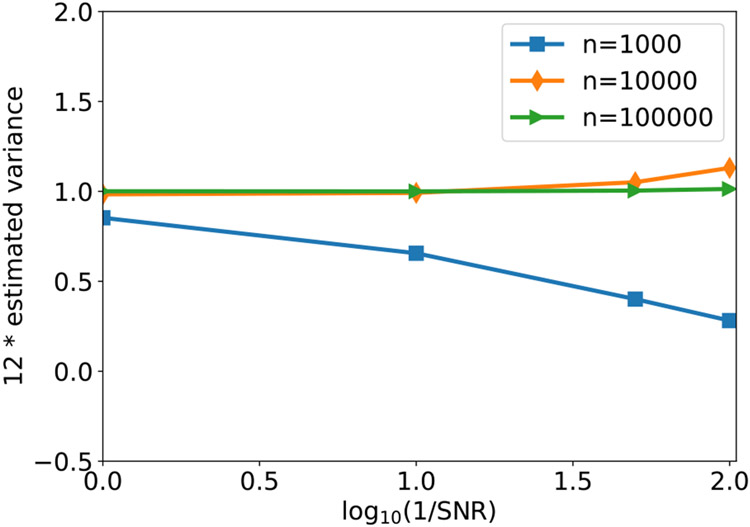
We next examine the performance of our estimator of contrast variance (12) under different SNRs and number of images. Since our simulated contrasts are uniformly distributed on [0.5, 1.5], the ground truth variance is 1/12, and thus ideally the line plots in Fig. 2 should align with the horizontal line y = 1. For small number of images n = 1000, our method often underestimates the variability of contrast, especially under low SNR. In this regime, our method mainly captures the magnitude of image noise, which is indeed assumed as approximately a constant (so variance is small) across images. For medium size of n, namely n = 10000, our method gives good estimate of contrast variance at SNR= 1, 0.1, but tends to overestimate it when SNR goes lower. In this regime, the overestimation is mainly due to the inaccurate estimation of μ and Σ_cx. Ideally, in the absence of noise, μ and Σ_cx1 should be parallel to each other due to (11). When $\widehat{\mu }$ and ${\widehat{\Sigma }}_{cx}1$ are far from being parallel, then one would expect a larger Var(c) to minimize the energy in (12). We finally remark that when n = 10⁵, we are able to accurately estimate Var(c) for SNR as low as 1/100.

Fig. 2.

The estimated variance of contrasts with varying SNR and number of images n. The image noise is white Gaussian. The ground truth value of the y-axis is 1, because the image contrasts are sampled from the uniform distribution on [0.5,1.5].

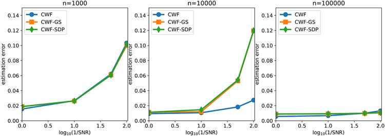
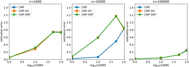
We next check the estimation of the covariance matrix Σ_cx. In Fig. 3, we present the line plot of the normalized estimation error $e_{\Sigma }≔\Vert {\widehat{\Sigma }}_{cx}-{\Sigma }_{cx}{\Vert }_F^2∕\Vert {\Sigma }_{cx}{\Vert }_F^2$. We observe from Fig. 3 that the estimation error of the refined covariance matrix strongly depends on the estimation error of Var(c). Indeed, when n = 10000 and SNR= 1/50 and 1/100, e_Σ of CWF-GS and CWF-SDP are both significantly larger than that of CWF. This large error is mainly due to the inaccurate estimation of the contrast variance at those SNRs. Our refined covariance matrices are more accurate under low SNR and large n, such as SNR= 1/100 and n = 10⁵ where Var(c) is accurately estimated. We show in Figs. 3-6 that although the refinement of covariance matrices does not necessarily reduce the estimation error, it plays a critical role for accurate contrast estimation.

Fig. 3.

Normalized error of covariance estimates by different methods. The image noise is white Gaussian.

Fig. 6.

Scatter plots of estimated contrasts v.s. true contrasts. n = 1000, SNR = 0.1. The image noise is white Gaussian. Ideally each scatter plot should align well with the line y = x.

To visualize the quality of contrast estimation by different methods, we present scatter plots of estimated contrasts v.s. ground truth ones. Ideally, the points in scatter plots should align well with the line y = x. We first show in Fig. 4 the scatter plots of different methods when n = 10000 and SNR = 1. “CWF-Oracle” refers to the CWF method with ground truth mean and covariance. We note that the oracle is the best linear estimator of the contrast. Our CWF-GS and CWF-SDP perform similarly and both of them achieve near-oracle accuracy for contrast estimation, and they are significantly better than the plain CWF.

Fig. 4.

Scatter plots of estimated contrasts v.s. true contrasts. n = 10000, SNR = 1. The image noise is white Gaussian. Ideally each scatter plot should align well with the line y = x.

Next, in Fig. 5 we keep the number of images fixed and lower the SNR to 0.1. All algorithms perform significantly worse than the results of SNR = 1. However, CWF-GS and CWF-SDP produce more accurate contrast estimates than those of plain CWF and are comparable to the oracle, which is consistent with Fig. 4.

Fig. 5.

Scatter plots of estimated contrasts v.s. true contrasts. n = 10000, SNR = 0.1. The image noise is white Gaussian. Ideally each scatter plot should align well with the line y = x.

Next, we show that the number of images often does not significantly affect the performance of our methods. That is, unlike CWF, our method does not require a large sample size for estimating the contrasts. In Fig. 6, we reduce the number of images to 1000 while keeping SNR = 0.1. The contrast estimation by the plain CWF is much less accurate after reducing the number of images. In contrast, our methods better maintain the quality of contrast estimates after reducing n. This suggests that our method is more robust to inaccuracies of the estimated covariance matrix.

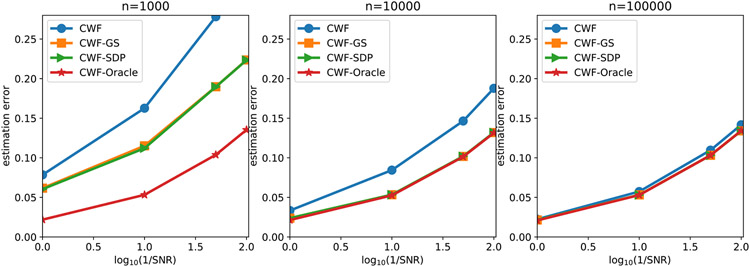
In Fig. 7 we compare the contrast estimation error of different methods under different SNRs and number of images. We use the averaged relative error

$$e_c=\frac{1}{n}\sum _{i=1}^n\mid \frac{{\widehat{c}}_i-c_i}{c_i}\mid$$ (24)

to measure the performance of the contrast estimation. We limit the y-axis of the line plot on the interval [0, 0.28] since any contrast estimation error above 0.28 is regarded as non-informative. Indeed, a trivial contrast estimator that estimates every c_i as 1 would give the error close to 0.28 in expectation. We observe that when n = 10000, although the covariance matrices are not very accurately estimated, CWF-GS and CWF-SDP both achieve performance that is comparable to the oracle. However, CWF needed 100000 samples to reduce the gap to the oracle. Even with n = 100000, CWF is still slightly worse than the oracle and our methods. Therefore, the key factor that determines the quality of contrast estimation is not how covariance is close to the true one, but is whether the covariance is enforced to satisfy the constraints stated in Proposition 1.

Fig. 7.

Contrast estimation error under different SNRs and number of images. The image noise is white Gaussian.

Next, we test the performance of the algorithms on image denoising. We compare the plain CWF and the ones with our refined covariances. We also compare the denoised images with image normalization and our 2-stage CWF procedure, introduced in Section 3.5. The two previous methods we compare are CWF and CWF-norm [4]. The latter one is the CWF with an image normalization step. The labels “-GS” and “-SDP” refer to usage of the refined covariance matrix (estimated by our GS procedure and SDP method) for CWF.

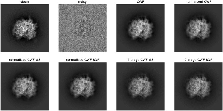
Before presenting the estimation errors, we show an example of clean and noisy images and denoised ones by different methods. In this example, SNR = 0.1 and n = 10000. From the result of Fig. 8, the denoised image by the original CWF with normalization looks similar to the ones by our normalization methods, although they have slightly different contrasts. The denoised images by our 2-stage methods have clearer fine details than those that are denoised by other methods.

Fig. 8.

Clean, noisy and denoised images with SNR = 0.1 and n = 10000. The image noise is white Gaussian.

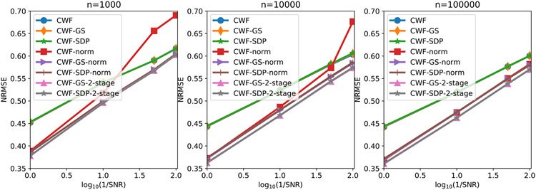
We evaluate the denoising performance by the normalized root mean squared error (NRMSE) within a circular mask whose radius is half the image size. From Fig. 9, CWF with image normalization often gives large errors under low SNR and small to medium n. Our image normalization and 2-staged methods consistently perform better than CWF and CWF-normalization, where 2-staged methods are slightly better. We also observe that our GS and SDP refinement yield similar estimation errors, where GS is slightly better under low SNRs.

Fig. 9.

NRMSE of the denoised images under different SNRs and the number of images. The image noise is white Gaussian.

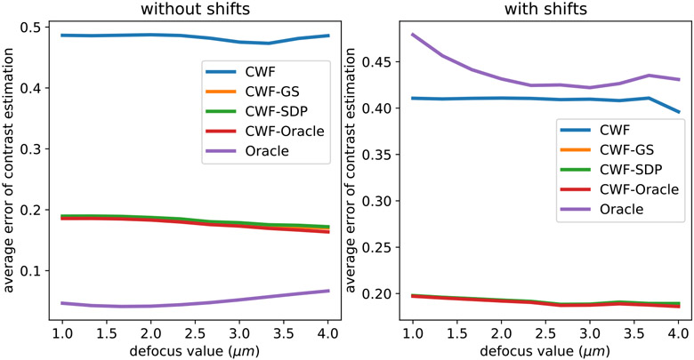
We further examine the contrast estimation error in each defocus group. In Fig. 10 we compare the contrast estimation errors of different methods in each of the 10 defocus groups for n = 10000 and SNR = 0.1. The defocus groups are sorted by defocus values in ascending order. In addition to the previously tested methods, we include a stronger oracle that knows the true clean images (not just true covariance). It estimates the contrast by $\widehat{c_i}=\langle {\mathit{y}}_i,A_i{\mathit{x}}_i\rangle ∕\Vert A_i{\mathit{x}}_i{\Vert }_2^2$. We refer to this method as “Oracle”. On the right panel of Fig. 10 we test the contrast estimation when the observed noisy images are randomly shifted by 1–5 pixels in x and y directions. From Fig. 10, the contrast estimation errors of both CWF and our methods tend to decrease when the defocus value increases. This makes sense, since CTFs with larger defocus values have higher absolute values around the zero-th frequency, and thus enjoy higher SNRs at low frequencies. When all images are centered, the “oracle” indicates the best possible contrast estimation that a template-based method can achieve, which obviously outperforms all other methods including the CWF-oracle. We remark that “oracle” knows the true manifold of the clean images, whereas “CWF-oracle” assumes a linear approximation of it. However, the new oracle is not robust to shifts, unlike other methods. When the noisy images are shifted, the oracle, assuming it does not know the shifts in the observation and only computes the dot product between the shifted y_i and centered A_ix_i, gives poor contrast estimation. To mitigate this issue, a low pass filter to y_i and A_ix_i is often needed.

Fig. 10.

Average error per defocus group of contrast estimation by different methods. n = 10000, SNR = 0.1. The image noise is white Gaussian. The left figure panel uses centered noisy images. In the right panel, we randomly shifted the noisy images by 1–5 pixels in the x and y directions independently. In both panels, the two lines corresponding to CWF-GS and CWF-SDP overlap with each other.

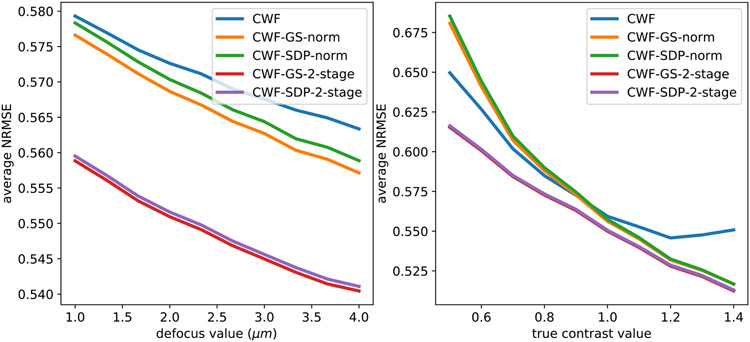
At last, in the left panel of Fig. 11, we compare the NRMSE of the denoised images by CWF with image normalization and our methods for each defocus group. On the right panel we show the relationship between the NRMSE of the denoised images and their contrast values. In particular, we divide the images into 10 groups by their true contrast values. Namely, the images with contrasts between 0.5 and 0.6 are classified as the first contrast group, and those with contrasts 0.6-0.7 are considered the second group and so on. We do not show CWF with image normalization since it has significantly higher NRMSE than other methods and will screw the scale of the y-axis. From the figure, for all methods, the NSMSEs often decrease when defocus values and contrast values increase. This agrees with our argument that higher defocus and contrast correspond to higher SNRs at low frequencies. However, with higher defocus values, more energy of clean signals is spilled outside of the image disk [28], and CTFs have more zero-crossings, which may have negative effects on image denoising. Indeed, we notice that when defocus values approach 4 μm, the NRMSEs slightly increase. Overall, the 2-stage methods perform significantly better than other methods.

Fig. 11.

Average NRMSE of denoised images from different methods, per defocus group (left figure) and per contrast group (right figure). n = 10000, SNR = 0.1. The image noise is white Gaussian. In the right panel, the red and purple lines overlap with each other.

4.2. Synthetic data with colored noise

We retest different methods on synthetic data with colored noise. The data generation procedure is exactly the same as before, except that now we use colored noise whose power spectrum decays with the radial frequency. Colored noise is more realistic in the sense that it better mimics the noise statistics observed in experimental images. Our choice of colored noise makes contrast estimation more challenging. Indeed, given the noise spectrum $1∕\sqrt{k^2+1}$ (up to a constant) where k is measured in 1/(128 pixel size), under the same SNR, the noise power spectrum in the zeroth frequency is expected to be 40 times larger than that of the white noise. Since contrast (mean of the pixels) is all about the zeroth frequency, the high noise at low frequencies poses a serious challenge.

Figure 12 shows an example of a clean image and noisy ones at different SNRs. Comparing with Fig. 1, the particles are harder to identify by human eyes than in the case of white noise. Indeed, starting from SNR=0.1, it already becomes hard to visually distinguish the particle from the colored noise in the background.

Fig. 12.

An example of clean and noisy images with colored noise. The defocus value for the CTF of the noisy images in this example is 2.67 μm.

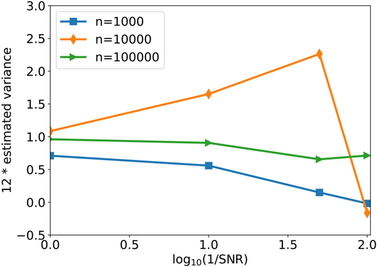
We next test the variance estimation for the contrasts. As shown in Fig. 13, the performance of the variance estimation is indeed worse than that for images with white noise. For n = 1000, our method consistently underestimates the variance. For n = 10000, there is an interesting transition from overestimation to underestimation between SNR= 1/50 and 1/100. This is likely due to that at SNR= 1/100, our method starts to learn the variance of the average pixel values of noise which is close to 0. However, for n = 100000, we are able to reliably estimate Var(c) up to SNR = 0.1.

Fig. 13.

The estimated variance of contrasts with varying SNR and n. The image noise is colored Gaussian with decaying PSD. The ground truth of the y-axis is 1.

Figure 14 shows the covariance estimation error for the different methods. Similar to the white noise case, the large errors of our methods when n = 10000 are mainly due to overestimation of Var(c), We notice a slight drop of covariance estimation error at SNR= 0.01 when n = 10000. This is due to the reduced error of contrast variance estimation (see the orange line in Fig. 13). However, as we show next, these refined covariance matrices are key for accurate contrast estimation.

Fig. 14.

Normalized error of covariance estimates by different methods. The image noise is colored Gaussian with decaying PSD. The line of CWF does not appear in the left panel due to its high error. In the right panel, the line of CWF overlaps with the lines of other methods.

As before, we assess the quality of the contrast estimation through scatter plots. From the result of Fig. 15, all methods perform significantly worse than in the white noise case. However our methods are still comparable to the oracle one and are considerably better than the original CWF.

Fig. 15.

Scatter plots of estimated contrasts v.s. true contrasts. n = 10000, SNR = 1. The image noise is colored Gaussian with decaying PSD.

Next, we fix n and decrease SNR to 0.1. In Fig. 16, the original CWF almost fails since there is no clear linear association between its estimated contrasts and the true ones. However, one can see a clear trend between the contrasts estimated by our methods and the ground truth ones. Again, our methods achieve comparable accuracy to the oracle one.

Fig. 16.

Scatter plots of estimated contrasts v.s. true contrasts. n = 10000, SNR = 0.1. The image noise is colored Gaussian with decaying PSD.

We next keep the SNR and reduce the number of images to 1000. In Fig. 17, the performance gap between our methods and CWF is even larger, and our methods are still comparable to the oracle. In both Fig. 16 and 17 the scatter plots of our methods tend to follow a straight line with a smaller slope, due to the high noise. Indeed, consider the extreme case of pure noise images, the estimated contrasts should follow a horizontal line.

Fig. 17.

Scatter plots of estimated contrasts v.s. true contrasts. n = 1000, SNR = 0.1. The image noise is colored Gaussian with decaying PSD.

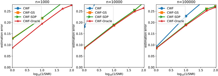
In Fig. 18 we compare the contrast estimation error of different methods under different SNRs and number of images. We observe that the CWF-GS and CWF-SDP both perform comparably to the oracle for n ≥ 10000. They also perform close to the oracle for the small sample size n = 1000, which indicates their robustness to the sample size unlike CWF. When n = 1000, the error of CWF is always above 0.28, thus it does not appear in the plot. There is still a large gap between CWF and our methods (and oracle) when n = 100000.

Fig. 18.

Contrast estimation error under different SNRs and number of images. The image noise is colored Gaussian with decaying PSD.

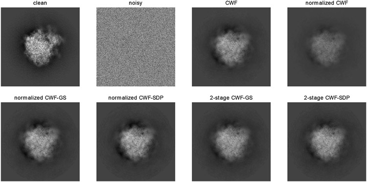
As for image denoising, we first show an example of clean and noisy images and denoised ones by different methods. In this example, SNR = 0.1 and n = 10000. From the result of Fig. 19, the denoised image by the original CWF with normalization gives much lower contrast than the ones by our normalization methods. The denoised images by our 2-stage methods seem to have clearer fine details than those that are denoised by other methods.

Fig. 19.

Clean, noisy and denoised images with SNR = 0.1 and n = 10000. The image noise is colored Gaussian with decaying PSD.

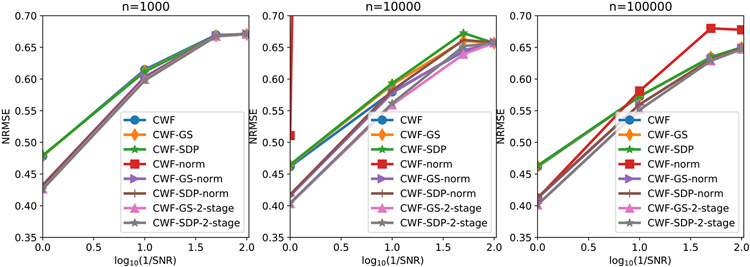
Next, we compare the NRMSE of the denoised images by the different algorithms. From Fig. 20, CWF with image normalization is very unstable. It does not appear in the first subplot due to exceeding the y-axis limit. Similar to the white noise case, our image normalization and 2-staged methods often have smaller errors than other methods, where 2-staged methods are slightly better. Similar to the white noise case, our GS refinement yields slightly smaller estimation errors than the SDP method under low SNRs.

Fig. 20.

NRMSE of the denoised images under different SNRs and number of images. The image noise is colored Gaussian with decaying PSD.

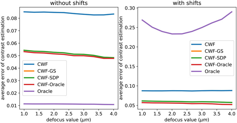
Similar to the white noise case, we examine the relationship between contrast estimation errors and the defocus values of the corresponding CTFs. In Fig. 21 we compare the average contrast estimation errors of different methods in each of the 10 defocus groups. The defocus groups are sorted by defocus values in ascending order. On the right of Fig. 21 we test the contrast estimation when the observed noisy images are randomly shifted by 1–5 pixels in the x and y directions. From Fig. 21, the contrast estimation errors of both CWF and our methods tend to decrease when defocus value increases. The instability of the “oracle” method to the shifts of images is also observed.

Fig. 21.

Average error per defocus group of contrast estimation by different methods. n = 10000, SNR = 0.1. The image noise is colored Gaussian with decaying PSD. The left panel uses centered noisy images. In the right panel, we randomly shift noisy images by 1–5 pixels in the x and y directions independently. In the right panel, the lines corresponding to CWF-GS and CWF-SDP overlap with each other.

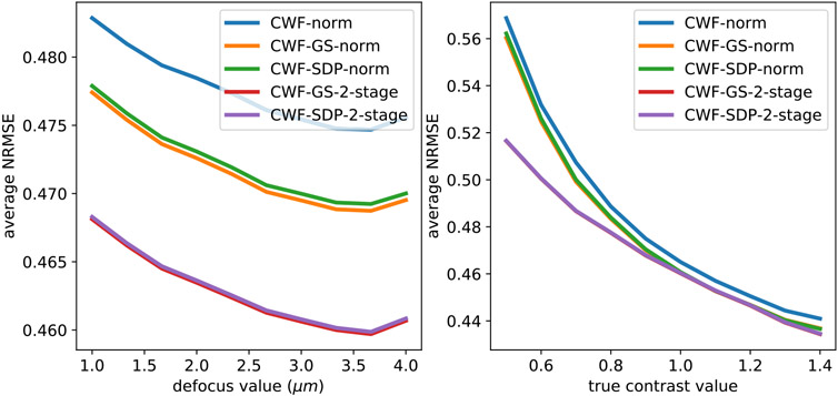
Same as the white noise case, in the left panel of Fig. 22, we compare the NRMSE of the denoised images by CWF and our methods within each defocus group. The right panel shows the relationship between NRMSE of denoised images and their contrast values. From the figure, for all methods, the NSMSE often decreases when defocus value and contrast value increase. The results of this section suggest that the 2-stage methods outperform the other CWF-based methods, and we therefore expect them to be the method of choice also for experimental data.

Fig. 22.

Average NRMSE of denoised images from different methods, per defocus group (left panel) and per contrast group (right panel). n = 10000, SNR = 0.1. The image noise is colored Gaussian with decaying PSD.

5. Results for experimental data

We compare our methods with CWF on three experimental datasets, which are freely downloadable from the Electron Microscope Pilot Image Archive (EMPIAR) database [14]. We chose these datasets for a purely technical reason, as each micrograph in these datasets has a single CTF, which reduces the total number of CTFs and runtime of our method. For the datasets where each image has its own CTF, it is possible accelerate our method by implementing in 2-D Fourier space the operations that involve the CTFs. However, to keep the idea of this work clean and focused, we leave this modification to future work. Due to the similar performance of our methods on the the three datasets, in this section we only present the result for EMPIAR-10028 [35], and refer the reader to the supplementary material for the results for EMPIAR-10005 [16] and EMPIAR-10073 [18].

For all datasets, we first normalize each individual image by the standard deviation (std) of the pixel values at the image corners that are located outside a circular mask with radius 0.45L, where L is the dimension of the square image. Next, for each defocus group we estimate the PSD of the noise in the normalized images, using the pixel values outside of the same mask. We then perform background subtraction by subtracting the mean of pixel values outside the mask. For each defocus group, the images are whitened by applying the single whitening filter that equals to the −0.5 power of the estimated noise PSD of that defocus group. By doing this, we are assuming that the images in the same micrograph have similar noise PSDs, in order to reduce the estimation error of the noise PSD which could be quite large for a single image. Moreover, whitening by defocus group accelerates our algorithm. In particular, given the whitened image formation model W_iy_i = c_iW_iA_ix_i + W_iϵ_i, to recover x_i we use the whitened CTFs W_iA_i. Using distinct whitening filter W_i for all images increases the number of distinct CTFs and the computational complexity of the existing implementation of CWF. We also note that we have to estimate the PSD before the background subtraction, otherwise the estimated PSD will vanish at the zeroth frequency and cause numerical issues when whitening the image. The possibly inaccurately estimated PSD, together with imperfect centering of particles and the ignored astigmatism in CTF, may cause imperfect CTF correction and additional blurring in the restored images. However, we demonstrate in our experimental results that our methods are more robust to these factors than the original CWF, especially for contrast estimation. The machine and the number of cores we used for the experimental datasets are the same as those of the synthetic simulations.

5.1. EMPIAR-10028

We test the algorithms on a dataset of the Plasmodium falciparum 80S ribosome bound to the anti-protozoan drug emetine. The picked particles are downloadable from EMPIAR-10028 [35]. Its 3-D reconstruction can be found on EMDB as EMD-2660 [35]. The dataset consists of 105247 motion corrected and picked particle images of size 360 × 360 with 1.34 Å pixel size, from 1081 defocus groups. We estimate the covariance using all images, and use 21 defocus groups to estimate the contrast of individual images and then denoise the selected images. The background subtraction, whitening, Fourier-Bessel expansion and covariance estimation took 10 h. It took 5 s for SDP covariance refinement and less than 1 s for the GS one. We apply Wiener filtering to 21 defocus groups, which take 11 min. Contrast estimation from the Fourier-Bessel coefficients took less than one second.

We first examine the relationship between the contrasts of particle images and their locations in a micrograph. Since the ground truth clean contrasts are not available, we use the approximate ground truth contrasts that are obtained from template matching with clean projections of the 3-D volume estimated by RELION (available in EMD-2660). In order to do this, we first generate 1000 clean templates that are projected from uniformly distributed viewing directions. Next, for each particle image, we find its viewing direction, 2-D in-plane rotation and shift by aligning its CWF-denoised image with each of the clean template by the method of [22]. We found that using the denoised images often provide more accurate alignment than using the raw images. To compute the oracle contrast of each noisy image Y_i, we apply its CTF to the aligned clean template and obtain ${\mathit{Y}}_i^{\ast }$. However, the contrast directly computed by

$$c_i^{\ast }=\langle {\mathit{Y}}_i,{\mathit{Y}}_i^{\ast }\rangle ∕\Vert {\mathit{Y}}_i^{\ast }{\Vert }_F^2$$

can be sensitive to even slight errors in alignment, as we demonstrated in Figs. 10 and 21 in synthetic data simulations. To mitigate this issue, we apply Gaussian smoothing to both Y_i and ${\mathit{Y}}_i^{\ast }$ before computing the “ground truth” contrast using the above formula. We choose an envelope function with a B-factor 1000 as our Gaussian filter. We remark that the clean projections are only used to generate approximate ground truth for evaluation, and are not used in CWF and our methods.

Each subplot of Fig. 23 corresponds to one micrograph, where each dot represents a picked particle image in that micrograph. The location of the dots are the location of the particle images in that micrograph, whose color represents the oracle contrast by template matching. The defocus values of the three micrographs (from left to right) are respectively 0.8131 μm, 1.9676 μm, and 2.6643 μm. Figure 23 suggests the existence of local correlations of image contrasts. Indeed, many pairs of nearby particles have very similar contrasts. However, the correlation of contrasts is only present within very small sub-regions of the micrograph.

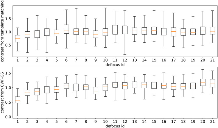
We next present a box plot of both oracle contrasts (top subplot) and the contrasts estimated by CWF-GS (bottom subplot) for each of the 21 defocus groups in Fig. 24. We ignore the result from CWF-SDP as it is very similar to the one of CWF-GS. We also ignore the result from CWF, since its contrast estimation is not accurate (see later in Fig. 25) and thus its box plot is not informative. From left to right in each subfigure, the defocus values are sorted in ascending order, ranging from 0.8131 μm to 2.6643 μm. In each box plot, the 5 horizontal lines, from top to bottom, respectively correspond to max value, 75% quantile, median, 25% quantile and min value. The two box plots are similar, even though their contrasts are estimated using completely different methods. One can also see a clearer trend from the second subfigure (our method) that micrographs with higher defocus values tend to have higher contrast. This makes sense, as CTFs with higher defocus values preserve more low frequency information, which yields higher SNR in low frequencies. Interestingly, both subfigures show that contrast variation within each micrograph is often larger than the variance of the median contrast of each micrograph (the variance of the y-values of the orange lines). This possibly indicates that using a single contrast value per micrograph, as assumed in the 3-D iterative refinement stage, is not appropriate.

Fig. 24.

Box plot of the oracle contrasts (top) and our estimated contrasts (bottom) in 21 defocus groups of the dataset EMPIAR-10028. The defocus values are sorted in ascending order, ranging from 0.8131 μm to 2.6643 μm.

Fig. 25.

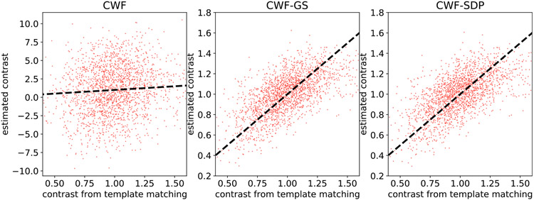
The scatter plots of the estimated contrast v.s. the oracle contrast for three defocus groups in the dataset EMPIAR-10028. The dashed line corresponds to the function y = x.

Next, we present the scatter plot between the estimated contrasts and the oracle contrast.

It is clear from Fig. 25 that our estimates have much better correlation with the oracle. We remark that we do not expect a strong correlation in any case, since the oracle itself is noisy and suffers from imperfect alignment. However, this is strong evidence that our methods provide much better contrast estimates than CWF.

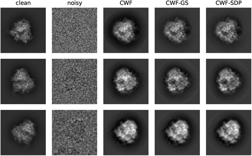
We next compare the image denoising performance by CWF and the ones with our refined covariance matrix. Since image normalization only affects the global scale of the image and normalized CWF performs poorly, we only show the denoised images without normalization. We also found that the 2-stage CWF often performs worse than the 1-stage version, possibly due to violation of assumptions in our synthetic model, such as imperfect centering and astigmatism in CTF. Thus, we recommend applying the one-stage algorithm for experimental datasets, and we compare their denoised images as follows. From Fig. 26, all methods produce dark areas around the boundary of the particle. These dark rings are likely due to the imperfect CTF correction by CWF. The denoised images by our methods have less dark areas, comparing to that of CWF. Since negative pixel values are often observed in CTF-affected clean images, these dark rings in CWF-denoised images are possibly due to inaccurate CTF-correction, which suggests better CTF correction by our methods. Furthermore, we observe better denoised images by our methods with closer contrast to the clean templates (Fig. 27).

Fig. 26.

Denoising results of EMPIAR-10028.

Fig. 27.

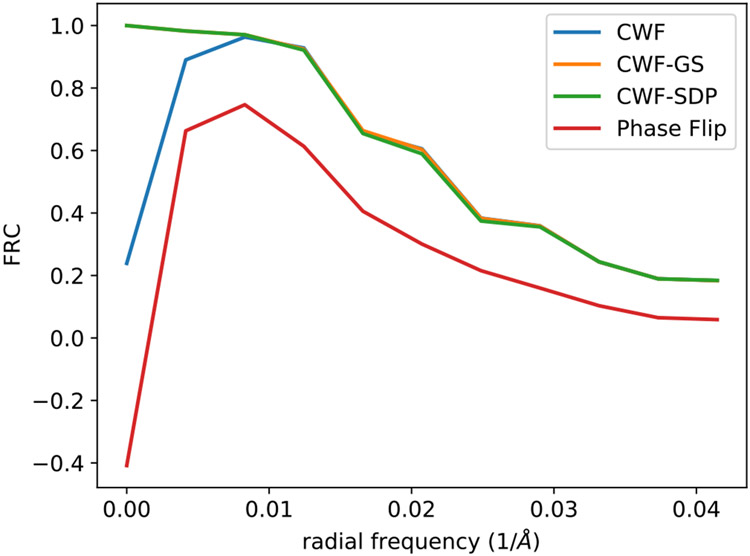
The average Fourier ring correlation between denoised images and the aligned clean templates over 2015 images from EMPIAR-10028.

At last, to quantitatively compare the denoising results of different methods, we compute the Fourier ring correlations (FRC) between the denoised images and their aligned clean templates. That is, for each pair of two images I₁ and I₂ and their Fourier coefficient vectors f_1,r, f_2,r at radial frequency r, we compute

$$\text{FRC}(r)=\frac{\Re ({\mathit{f}}_{1,r}^{\ast }{\mathit{f}}_{2,r})}{\Vert {\mathit{f}}_{1,r}\Vert \Vert {\mathit{f}}_{2,r}\Vert },$$

where 𝕽 denotes taking the real part of a complex number. For each method, we compute the average FRC between the denoised images and the clean templates over the 2015 images from 21 defocus groups. We notice that FRC is very sensitive to image rotations and shifts. With slight error in image alignment, the FRC of all methods decreases rapidly as r increases. As a result, when alignment errors are present, FRC may not reflect the true image quality. However, even from the first few frequencies, the FRCs of CWF-based methods are much higher than that of the naïve phase flipping method. We also notice that CWF-denoised images have large errors in the first two frequencies, mainly due to its limitations in handling contrast variations. Since the clean templates are only aligned and registered with CWF-denoised images, the comparison is a bit unfair to our methods, as our methods may suffer from larger alignment errors. However, even in this scenario, our methods achieve much better FRC at the first two radial frequencies due to the better contrast estimation.

6. Conclusion

We introduced an effective algorithm for estimating the amplitude contrast of individual images and the overall contrast variability in the ab-initio stage. Our method refines the initial estimated covariance so it satisfies additional constraints that follow from the image formation model by tomographic projection. Results for both synthetic and experimental datasets indicate consistently better contrast estimation by our methods than CWF. On synthetic data, the contrast estimation errors of our methods are comparable to those of an oracle, even with small number of images. We also demonstrate that our method improves the image denoising result of CWF. Among the various contrast estimation and image denoising techniques that were considered in this paper, following the results for experimental datasets we recommend using CWF-GS (see Algorithm 1 with option=GS in Section 3.7) for contrast estimation and CWF-GS with image normalization for image denoising (see Algorithm 2 with option=normalization in Section 3.7). There are also some interesting future directions. For example, one can try techniques based on common-lines to directly estimate the rotations of molecules by using the denoised and normalized images from our methods with rudimentary 2-D class averaging [2]. Normalizing the images may also lead to improvement of 2-D class averaging procedures. An-other interesting application of our method is to use our estimated contrasts to initialize their values in the iterative refinement procedure of RELION [24]. As for the computational aspect, one can modify the original CWF method so it can more efficiently handle per-image CTF, rather than a small number of defocus groups. Our Python code is available at https://github.com/yunpeng-shi/contrast-cryo which is planned to be integrated into ASPIRE [36].

References

- [1].Bai X-C, McMullan G, Scheres SH, How cryo-EM is revolutionizing structural biology, Trends Biochem. Sci 40 (1) (2015) 49–57. [DOI] [PubMed] [Google Scholar]
- [2].Bandeira AS, Chen Y, Lederman RR, Singer A, Non-unique games over compact groups and orientation estimation in cryo-EM, Inverse Probl. 36 (6) (2020) 064002. [DOI] [PMC free article] [PubMed] [Google Scholar]
- [3].Bepler T, Kelley K, Noble AJ, Berger B, Topaz-denoise: general deep denoising models for cryoEM and cryoET, Nat. Commun 11 (1) (2020) 1–12. [DOI] [PMC free article] [PubMed] [Google Scholar]
- [4].Bhamre T, Zhang T, Singer A, Denoising and covariance estimation of single particle cryo-EM images, J. Struct. Biol 195 (1) (2016) 72–81. [DOI] [PMC free article] [PubMed] [Google Scholar]
- [5].Bhamre T, Zhao Z, Singer A, Mahalanobis distance for class averaging of cryo-EM images, in: 2017 IEEE 14th International Symposium on Biomedical Imaging (ISBI 2017), IEEE, 2017, pp. 654–658. [DOI] [PMC free article] [PubMed] [Google Scholar]
- [6].Cheng Y, Single-particle cryo-EM-how did it get here and where will it go, Science 361 (6405) (2018) 876–880. [DOI] [PMC free article] [PubMed] [Google Scholar]
- [7].Chung S-C, Lin H-H, Niu P-Y, Huang S-H, Tu I, Chang W-H, et al. , Pre-pro is a fast pre-processor for single-particle cryo-EM by enhancing 2-D classification, Commun. Biol 3 (1) (2020) 1–12. [DOI] [PMC free article] [PubMed] [Google Scholar]
- [8].Diamond S, Boyd S, CVXPY: a Python-embedded modeling language for convex optimization, J. Mach. Learn. Res 17 (83) (2016) 1–5. [PMC free article] [PubMed] [Google Scholar]
- [9].Fan Y, Zhao Z, Cryo-electron microscopy image denoising using multifrequency vector diffusion maps, in: 2021 IEEE International Conference on Image Processing (ICIP), 2021, pp. 3463–3467, doi: 10.1109/ICIP42928.2021.9506435. [DOI] [Google Scholar]
- [10].Frank J, Advances in the field of single-particle cryo-electron microscopy over the last decade, Nat. Protoc 12 (2) (2017) 209–212. [DOI] [PMC free article] [PubMed] [Google Scholar]
- [11].Gu H, Unarta IC, Huang X, Yao Y, Generative adversarial networks for robust cryo-EM image denoising, arXiv preprint arXiv:2008.07307(2022). [Google Scholar]
- [12].Heimowitz A, Andén J, Singer A, Reducing bias and variance for CTF estimation in single particle cryo-EM, Ultramicroscopy 212 (2020) 112950. [DOI] [PMC free article] [PubMed] [Google Scholar]
- [13].Helmberg C, Rendl F, Vanderbei RJ, Wolkowicz H, An interior-point method for semidefinite programming, SIAM J. Optim 6 (2) (1996) 342–361. [Google Scholar]
- [14].Iudin A, Korir PK, Salavert-Torres J, Kleywegt GJ, Patwardhan A, EMPIAR: a public archive for raw electron microscopy image data, Nat. Methods 13 (5) (2016) 387–388, doi: 10.1038/nmeth.3806. [DOI] [PubMed] [Google Scholar]
- [15].Landa B, Shkolnisky Y, The steerable graph Laplacian and its application to filtering image datasets, SIAM J. Imaging Sci 11 (4) (2018) 2254–2304. [Google Scholar]
- [16].Liao M, Cao E, Julius D, Cheng Y, Structure of the TRPV1 ion channel determined by electron cryo-microscopy, Nature 504 (7478) (2013) 107–112. [DOI] [PMC free article] [PubMed] [Google Scholar]
- [17].Moscovich A, Halevi A, Andén J, Singer A, Cryo-EM reconstruction of continuous heterogeneity by Laplacian spectral volumes, Inverse Probl. 36 (2) (2020) 024003. [DOI] [PMC free article] [PubMed] [Google Scholar]
- [18].Nguyen THD, Galej WP, Bai X.-c., Oubridge C, Newman AJ, Scheres SH, Nagai K, Cryo-EM structure of the yeast U4/U6.U5 tri-snRNP at 3.7 Å resolution, Nature 530 (7590) (2016) 298–302. [DOI] [PMC free article] [PubMed] [Google Scholar]
- [19].O’donoghue B, Chu E, Parikh N, Boyd S, Conic optimization via operator splitting and homogeneous self-dual embedding, J. Optim. Theory Appl 169 (3) (2016) 1042–1068. [Google Scholar]
- [20].Palovcak E, Asarnow D, Campbell MG, Yu Z, Cheng Y, Enhancing the signal-to-noise ratio and generating contrast for cryo-EM images with convolutional neural networks, IUCrJ 7 (6) (2020). [DOI] [PMC free article] [PubMed] [Google Scholar]
- [21].Penczek PA, Fang J, Li X, Cheng Y, Loerke J, Spahn CM, CTER–rapid estimation of CTF parameters with error assessment, Ultramicroscopy 140 (2014) 9–19. [DOI] [PMC free article] [PubMed] [Google Scholar]
- [22].Reddy BS, Chatterji BN, An FFT-based technique for translation, rotation, and scale-invariant image registration, IEEE Trans. Image Process 5 (8) (1996) 1266–1271. [DOI] [PubMed] [Google Scholar]
- [23].Rohou A, Grigorieff N, CTFFIND4: fast and accurate defocus estimation from electron micrographs, J. Struct. Biol 192 (2) (2015) 216–221. [DOI] [PMC free article] [PubMed] [Google Scholar]
- [24].Scheres SH, RELION: implementation of a Bayesian approach to cryo-EM structure determination, J. Struct. Biol 180 (3) (2012) 519–530. [DOI] [PMC free article] [PubMed] [Google Scholar]
- [25].Scheres SH, Valle M, Grob P, Nogales E, Carazo J-M, Maximum likelihood refinement of electron microscopy data with normalization errors, J. Struct. Biol 166 (2) (2009) 234–240. [DOI] [PMC free article] [PubMed] [Google Scholar]
- [26].Sigworth FJ, Principles of cryo-EM single-particle image processing, Microscopy 65 (1) (2016) 57–67. [DOI] [PMC free article] [PubMed] [Google Scholar]
- [27].Sigworth FJ, Doerschuk PC, Carazo J-M, Scheres SH, An introduction to maximum-likelihood methods in cryo-EM, Meth. Enzymol 482 (2010) 263–294. [DOI] [PMC free article] [PubMed] [Google Scholar]
- [28].Sindelar CV, Grigorieff N, An adaptation of the Wiener filter suitable for analyzing images of isolated single particles, J. Struct. Biol 176 (1) (2011) 60–74, doi: 10.1016/j.jsb.2011.06.010. [DOI] [PMC free article] [PubMed] [Google Scholar]
- [29].Singer A, Mathematics for cryo-electron microscopy, in: Proceedings of the International Congress of Mathematicians: Rio de Janeiro 2018, World Scientific, 2018, pp. 3995–4014. [Google Scholar]
- [30].Singer A, Sigworth FJ, Computational methods for single-particle electron cryomicroscopy, Annu. Rev. Biomed. Data Sci 3 (2020) 163–190. [DOI] [PMC free article] [PubMed] [Google Scholar]
- [31].Sorzano C, De La Fraga L, Clackdoyle R, Carazo J, Normalizing projection images: a study of image normalizing procedures for single particle three-dimensional electron microscopy, Ultramicroscopy 101 (2–4) (2004) 129–138. [DOI] [PubMed] [Google Scholar]
- [32].Spilman MS, Guo H, Bammes BE, Jin L, Bilhorn RB, Boosting contrast of cryo-EM images without a phase plate, Microsc. Microanal 21 (S3) (2015) 911–912. [Google Scholar]
- [33].Su M, Zhang H, Schawinski K, Zhang C, Cianfrocco MA, Generative adversarial networks as a tool to recover structural information from cryo-electron microscopy data, BioRxiv (2018) 256792. [Google Scholar]
- [34].Vulović M, Ravelli RB, van Vliet LJ, Koster AJ, Lazić I, Lücken U, Rullgård H, Öktem O, Rieger B, Image formation modeling in cryo-electron microscopy, J. Struct. Biol 183 (1) (2013) 19–32. [DOI] [PubMed] [Google Scholar]
- [35].Wong W, Bai X.-c., Brown A, Fernandez IS, Hanssen E, Condron M, Tan YH, Baum J, Scheres SH, Cryo-EM structure of the plasmodium falciparum 80s ribosome bound to the anti-protozoan drug emetine, Elife 3 (2014) e03080. [DOI] [PMC free article] [PubMed] [Google Scholar]
- [36].Wright G, Andén J, Bansal V, Xia J, Langfield C, Carmichael J, Brook R, Shi Y, Heimowitz A, Pragier G, Sason I, Moscovich A, Shkolnisky Y, Singer A, ComputationalCryoEM/ASPIRE-Python: v0.9.2. Zenodo; (2022). 10.5281/zenodo.5657282 [DOI] [Google Scholar]
- [37].Wu H, Zhai X, Lei D, Liu J, Yu Y, Bie R, Ren G, An algorithm for enhancing the image contrast of electron tomography, Sci. Rep 8 (1) (2018) 1–13. [DOI] [PMC free article] [PubMed] [Google Scholar]
- [38].Zhang K, Gctf: real-time CTF determination and correction, J. Struct. Biol 193 (1) (2016) 1–12. [DOI] [PMC free article] [PubMed] [Google Scholar]
- [39].Zhao Z, Shkolnisky Y, Singer A, Fast steerable principal component analysis, IEEE Trans. Comput. Imaging 2 (1) (2016) 1–12. [DOI] [PMC free article] [PubMed] [Google Scholar]
- [40].Zhao Z, Singer A, Rotationally invariant image representation for viewing direction classification in cryo-EM, J. Struct. Biol 186 (1) (2014) 153–166. [DOI] [PMC free article] [PubMed] [Google Scholar]
Associated Data
This section collects any data citations, data availability statements, or supplementary materials included in this article.