Abstract
Purpose:
Machine learning techniques can be applied to cardiac magnetic resonance imaging (CMR) scans in order to differentiate patients with and without ischemic myocardial scarring (IMS). However, processing the image data in the CMR scans requires manual work that takes a significant amount of time and expertise. We propose to develop and test an AI method to automatically identify IMS in CMR scans to streamline processing and reduce time costs.
Materials and Methods:
CMR scans from 170 patients (138 IMS & 32 without IMS as identified by a clinical expert) were processed using a multistep automatic image data selection algorithm. This algorithm consisted of cropping, circle detection, and supervised machine learning to isolate focused left ventricle image data. We used a ResNet-50 convolutional neural network to evaluate manual vs. automatic selection of left ventricle image data through calculating accuracy, sensitivity, specificity, F1 score, and area under the receiver operating characteristic curve (AUROC).
Results:
The algorithm accuracy, sensitivity, specificity, F1 score, and AUROC were 80.6%, 85.6%, 73.7%, 83.0%, and 0.837, respectively, when identifying IMS using manually selected left ventricle image data. With automatic selection of left ventricle image data, the same parameters were 78.5%, 86.0%, 70.7%, 79.7%, and 0.848, respectively.
Conclusion:
Our proposed automatic image data selection algorithm provides a promising alternative to manual selection when there are time and expertise limitations. Automatic image data selection may also prove to be an important and necessary step toward integration of machine learning diagnosis and prognosis in clinical workflows.
Keywords: Ischemic myocardial scarring, prognosis, diagnosis, neural network, cardiac, magnetic resonance imaging
1. INTRODUCTION
Coronary artery disease is a devastating presence in the lives of millions of people in the US and worldwide1. Ischemic myocardial scarring (IMS), a common sequela of coronary artery disease, is a condition which carries a potent risk for heart failure and lethal ventricular arrythmias. Computed tomography, magnetic resonance imaging, and echocardiograms are frequently used to identify IMS through the examination of cardiac morphology and function. However, full optimization of methods to accurately quantify IMS from the imaging data of these medical imaging modalities remains a focus of current and future research.
One of the most frequently used method of detecting IMS is gadolinium-enhanced cardiac magnetic resonance imaging (CMR). CMR with late gadolinium enhancement is commonly used for clinical decision-making and has known prognostic value. However, interpretation of CMR scans is a time-consuming process with a high expertise requirement. Thus, there remains a gap in clinical settings where machine learning could be applied in an attempt to achieve similar results to cardiologists, offering a valuable second opinion at times of diagnosis and prognosis.
To this end, several research groups have created machine learning algorithms to aid in this endeavor2–5. The source of image data for these algorithms encompasses different medical imaging modalities yet almost always focuses primarily on the left ventricle and surrounding myocardium. These regions of interest are where cardiologists seek to find information when trying to diagnose IMS. Figure 1 shows reference CMR images of patients without and with IMS.
Figure 1.
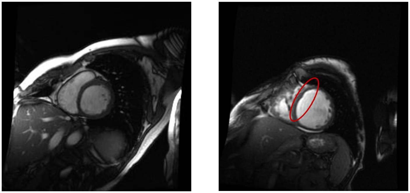
Reference images for no IMS (left) and IMS (right). The red oval in the right image indicates a region of scarring.
Despite machine learning being a logical avenue of approach to detecting IMS, there remain challenges localizing the most vital information in the data. These datasets, which often have hundreds or more images for a single patient, are not automatically focused on the best region for data extraction. On the contrary, the information is an aggregate bulk of information that is then analyzed by a cardiologist to make an expert decision. In order to apply machine learning, the data must therefore be focused on the correct region of the images in order to get a valid and timely result. In particular, with CMR scans, there is no easy way to automatically retrieve the region of interest image data from the scans while also integrating the clinical methods of cardiologists.
This suggests a need for an effective standardized way to extract and preprocess the most relevant data from CMR scans without manual intervention. Automation of this process would help provide clear avenues to integration of machine learning into the clinical workflow. Without this, the application of machine learning to the identification of IMS in clinical settings may never reach fruition.
In order to aid in this task, we have established an automated method of region of interest isolation that is able to handle bulk datasets. It applies computer programming guided by cardiologist methodology to isolate the left ventricle and the surrounding myocardium. With this heart region isolated, a machine learning convolutional neural network is trained to identify differences between control patient data and IMS patient data. The automated image data selection algorithm we have designed combined with a custom ResNet-50 convolutional neural network, was able to identify IMS with an accuracy of nearly 80%, within just a few percent of our manual data selection method which had an accuracy of just over 80%.
We believe that with the improvement of this method as well as a broader dataset, we would be able to offer a fast and accurate method for the clinical workflow to assist cardiologists in making diagnostic and prognostic decisions about IMS.
2. DATA
2.1. Data overview
The initial dataset was provided in the form of DICOM files which came from CMR scans done at a tertiary care facility. Data collection was approved by an institutional review board committee at the University at Buffalo. DICOMs provide a method of storing metadata and image data in a single file. For the purposes of this study, the metadata was used to organize, sort, and label the image data before then being discarded while retaining the extracted image data. This process was achieved using Python scripts enabled by the pydicom package6.
The images contained in the DICOM files were from a wide variety of scan types in resolutions of mostly 256×256 pixels. As short axis images provide the best view of the left ventricle and surrounding myocardium, short axis images were targeted for extraction from the DICOM files using the contained metadata. This resulted in 57,680 short axis images being extracted from the CMR scans of 170 patients (38 controls and 132 with IMS as classified by an expert cardiologist). Of these images, 11,320 are control images while 46,360 are images from IMS patients.
2.2. Data splitting
To facilitate a two-part machine learning process, the initial data was split into two major groups: D1 and D2. D1 contained 7,680 short axis images while D2 contained the remaining 50,000 short axis images. This split was necessary in order to first train machine learning to learn from the D1 data and then apply that learning to the D2 data.
Of note, the training and testing data in D1 and D2 were split by patient rather than by individual image. This was done due to the acquisition of the scans being done in sets of 20 at different elevations. Each of the 20 images differs slightly due to the temporal delta between them but is largely the same as their 19 other counterparts in the same set of 20. If these images were allowed to be present in both the training and testing datasets, then the machine learning would be able to discern the answer at close 100% accuracy but would not be broadly applicable to other sets of data.
3. METHODOLOGY
3.1. Methodology Overview
Our process includes isolation of short axis images from DICOMs, image cropping, machine learning filtering, circle detection, and additional image cropping. Through the series of steps depicted in Figure 2, we were able to create an automatic image data selection pipeline for left ventricle and surrounding myocardium image data from CMR scans.
Figure 2.
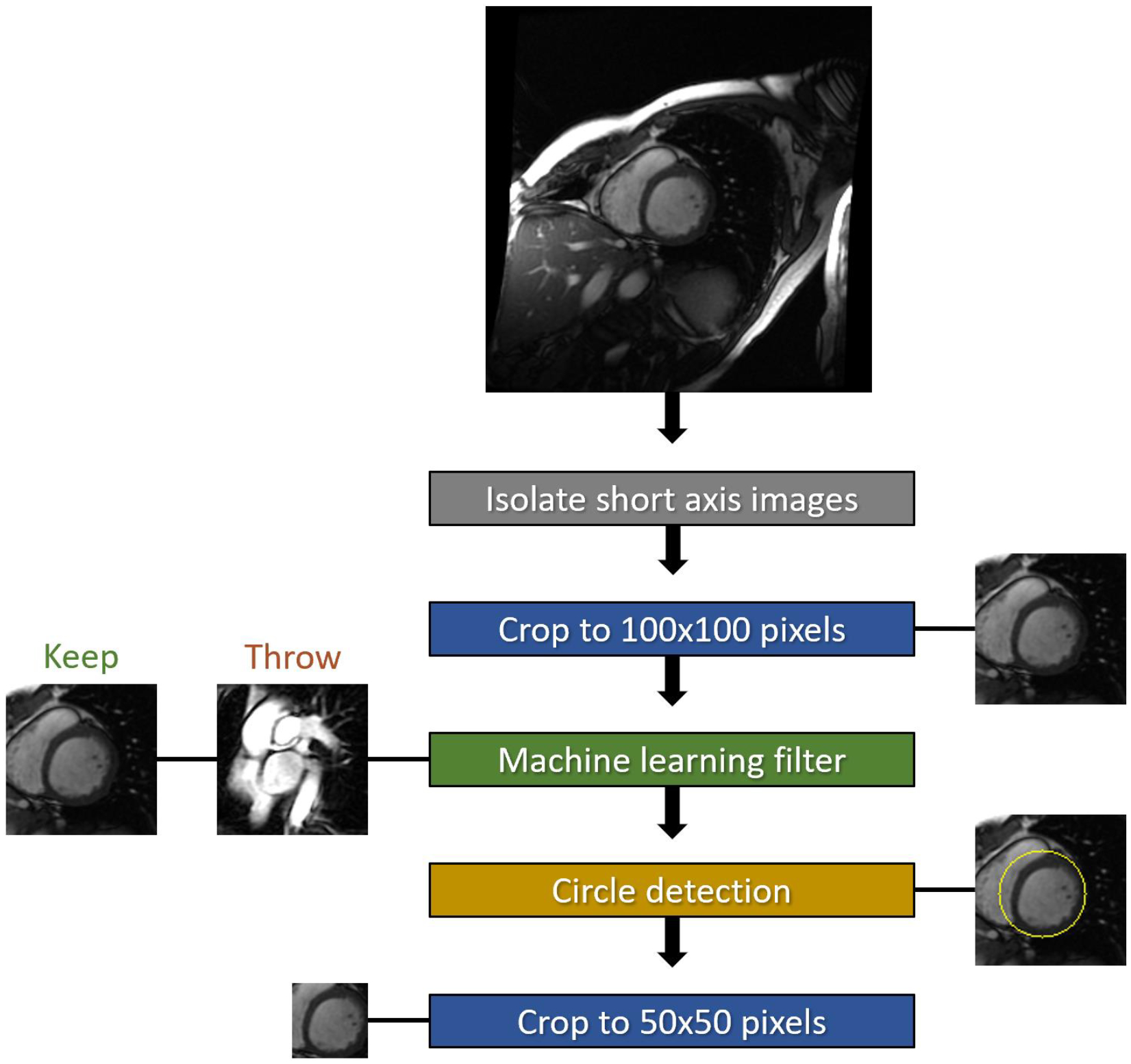
Automatic image data selection pipeline.
3.2. Size-reduction cropping
Due to the manner in which the CMR scans were acquired, the short axis images mostly had the heart region towards the center of the images. This allowed us to crop a 100×100 pixel region out of the center the 256×256 pixel images without losing a significant amount of heart image data (Figure 3). This process reduced our total pixels from 65,536 to just 10,000, greatly reducing the computational burden of the dataset and greatly increasing the specificity of the image data to the region of interest.
Figure 3.
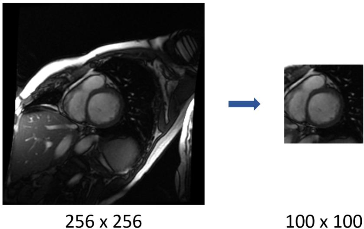
Initial reduction cropping. Reduction cropping aimed at capturing the heart allowed for greatly reduced pixel counts and thus reduced machine learning computational burden and increased region of interest specificity.
3.3. Keep & throw
The 100×100 pixel images from the D1 dataset with 7,680 short axis images was then sorted manually into two groups: keep and throw. Images in the keep group represented images with a clear view of the left ventricle and surrounding myocardium. Images designated to the throw category did not have a clear view of the left ventricle or had image artifacts. Sample keep and throw images are shown in Figure 4.
Figure 4.

Sample keep and throw images. The stark difference between the keep and throw images allowed the machine learning to apply the knowledge learned from the D1 dataset to the D2 dataset.
With the data sorted, machine learning using a ResNet-50 neural network was applied to find a clear differentiation between the images. Once this training was complete, a weight was saved from the training and applied to the D2 dataset. This greatly reduced the number of images that did not contain the desired information and resulted in the D2 dataset being reduced from 50,000 images to 16,484 images.
3.4. Hough circle transform
With a 100×100 pixel region isolated from each original scan and the machine learning applied to sort out undesired images, our next step was to apply Hough Circle Transform to best locate the left ventricle and surrounding myocardium7. This method of circle detection is available in the Python OpenCV package and detects edges and circularity8.
The circle detection was tuned to do 3 things using the parameters in Table 1:
Only find one circle
Focus on finding the left ventricle (or surrounding myocardium)
Focus on finding the most reliable data
Table 1.
Hough Circle Transform Parameters
| Parameter | Value |
|---|---|
| Hough gradient | 0.9 |
| min_dist | 150 |
| param1 | 50 |
| param2 | 25 |
| minRadius | 17 |
| maxRadius | 30 |
The major parameters involved in Hough Circle Transform are Hough gradient, min_dist, param1, param2, minRadius, and maxRadius. These variables describe the different aspects of how circular, how close together, how small or how big the detected circles are. By optimizing these parameters, we were able to locate single circles that most closely resembled our target left ventricle and surrounding myocardium. This also allowed us to minimize the number of circles missed and avoid many circle-like objects near the heart that were not the left ventricle and surrounding myocardium. Figure 5 shows an example of a circle detected in a 100×100 image of the heart sorted out as “keep” previously.
Figure 5:
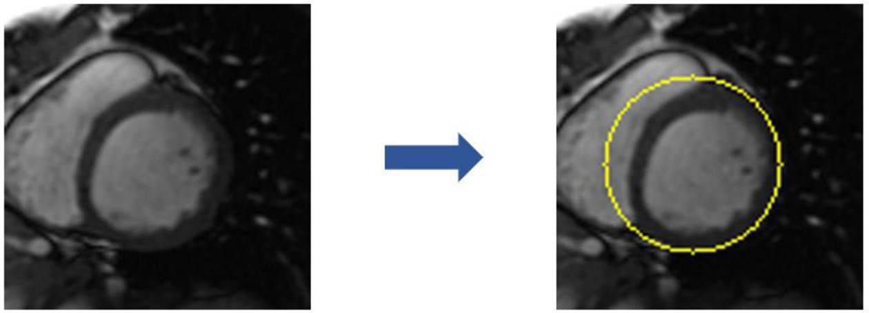
Circle detection on 100×100 pixel images. The circle detection is able to locate the left ventricle and the surrounding myocardium.
3.5. Cropping based on circle centers
With the circles detected, the coordinates for the center of the could then be used to crop out a significant amount of extraneous information outside of the left ventricle and surrounding myocardium. Figure 6 shows the result of using the center of the detected circle to create a 50×50 region of isolated left ventricle and myocardium.
Figure 6.
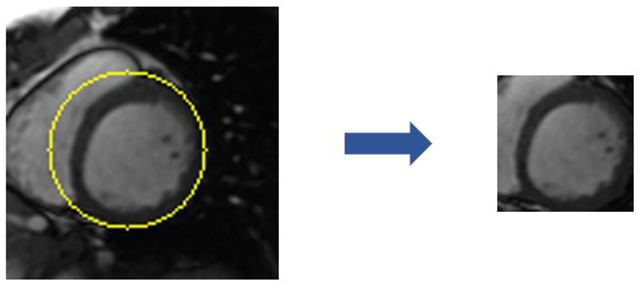
Circle-centered Reduction Cropping. Using the known coordinates of the center of the detected circle, image cropping can be performed on the image to reduce the size to 50×50 pixel square. This greatly reduces extraneous information found in the region surrounding the left ventricle and further reduces the computational burden.
In total, initial cropping combined with the circle-center reduction cropping take a 256×256 pixel image down to just 50×50 pixels which is a 96% reduction in the number of pixels. This greatly increased specificity to the region of interest.
3.6. Class balance
With the dataset containing images from 38 control patients and 132 patients with IMS, there was an imbalance between the classes which persisted into the reduced D2 dataset. In the reduced D2 dataset there were 3,298 images in the control group and 13,186 images in the IMS group. In order to correct for this class imbalance, we applied class weighting and rotated the control images 3 times. Doing so changed the balance to 13,192 control images and 13,186 IMS images.
Class weighting can be automated based on the size of the groups of data being put in and provides a minor correctional factor to imbalances seen with data being split up with stratified shuffle splits.
Further, given the circular nature of the left ventricle and surrounding myocardium, rotations seemed like a logical choice for improving class balance. Rotating the images was done using the rotate function of the Pillow package9. It allows for rotations at specified degrees. Note that mirroring is also possible with the Pillow package but was not used here.
Figure 7 shows sample rotations at 90°, 180°, and 270° degrees. Using multiples of 90° degrees allowed for the images to avoid being blurred or otherwise distorted by the rotations.
Figure 7.

Example Image Rotations. The original images were rotated at 90°, 180°, and 270° degrees.
3.7. Neural network selection
An appropriate neural network would have to apply a network layering strategy that is able to differentiate small detail changes as visually the heart structures remain similar between the control and disease states. With this in mind, we applied a ResNet-50 convolutional neural network to accomplish this task.
Of note, we also tried VGG16 and VGG19. Both networks were capable of differentiating the images into control and IMS sets. However, their overall performance was lower.
3.8. Model architecture design
Our problem is approached using the ResNet-50 convolutional neural network (Figure 8). Like other neural networks, the functionality can be augmented through the use of additional layers. The model architecture chosen makes use of large dense layers. Here, with small differences being key to success, the use of large(many-noded) dense layers hopefully provides the machine learning with more avenues of differentiation.
Figure 8.
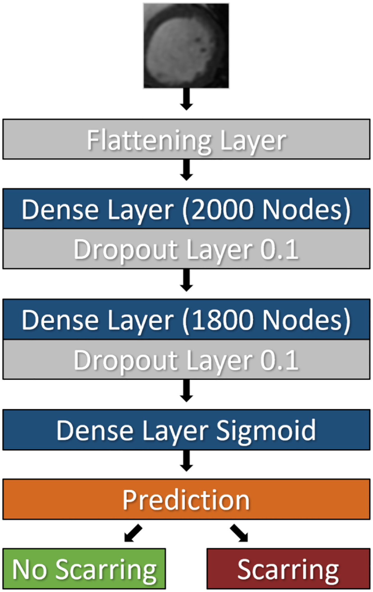
ResNet-50 Convolutional Neural Network Architecture.
3.9. Optimizer selection & parameter optimization
With the ResNet-50 convolutional neural network chosen, the next big choice was the optimizer. Optimizers provide a slew of tweakable parameters for use with neural networks in order to optimize their performance. Our choice was Follow The Regularized Leader (Ftrl)10. This optimizer has a few parameters that are not available in some other optimizers which lent it to further optimizations that were a good match for the complexity of the ResNet-50 architecture.
Within the scope of Ftrl, we chose to tune the learning rate, learning rate power, and initial accumulator value to optimize network performance (Table 2).
Table 2.
Ftrl Optimizer Parameter Selections and Epoch Counts for ResNet-50 Convolutional Neural Network
| Manual Selection | Automatic Selection | |
|---|---|---|
| Learning rate | 0.000183 | 0.000601 |
| Learning rate power | −0.61 | −0.73 |
| Initial accumulator value | 0.023 | 0.024 |
| Epochs | 7 | 13 |
3.10. Cross validation
For our cross validation we used the Stratified Shuffle Split function of the scikit-learn package for Python9. We chose to do our cross validation over 20 splits in order to help ensure result stability.
4. RESULTS
4.1. Performance Metric Results
Performance was measured through Accuracy, Sensitivity, Specificity, F1 Score, and area under the receiver operating characteristic curve (AUROC) with results shown in Table 3. The ResNet-50 convolutional neural network was able to achieve the best accuracy due to the higher sensitivity of the network. Manual selection with ResNet-50 achieved slightly above 80% accuracy while automatic selection with ResNet-50 was just below 80% accuracy. VGG19 and VGG16 had slightly lower performance with sensitivity being lower than with ResNet-50. Manual selection did better than automatic selection for both the VGG19 and VGG16 convolutional neural networks as well. Overall, all three convolutional neural networks had better specificity when using manual selection. AUROC was very stable across the board.
Table 3.
Performance Metrics for Convolutional Neural Networks
| Accuracy (%) | Sensitivity (%) | Specificity (%) | F1 Score (%) | AUROC | |
|---|---|---|---|---|---|
| ResNet-50 Manual | 80.6 | 85.6 | 73.7 | 83.0 | 0.837 |
| ResNet-50 Automatic | 78.5 | 86.0 | 70.7 | 79.7 | 0.848 |
| VGG19 Manual | 76.2 | 79.0 | 73.5 | 78.1 | 0.845 |
| VGG19 Automatic | 74.6 | 79.8 | 70.3 | 75.8 | 0.836 |
| VGG16 Manual | 75.6 | 78.9 | 72.0 | 77.1 | 0.842 |
| VGG16 Automatic | 75.1 | 79.4 | 71.5 | 76.0 | 0.841 |
4.2. Aggregate Receiver Operating Characteristic Curves
The ROC curves were created by taking the average value for 20 stratified k-fold splits with a ±1 standard deviation shaded blue region showing the variance of each curve with curves shown for all three convolutional neural networks for both manual and automatic selection seen in Figures 9, 10, and 11. AUROC (displayed as AUC in Figures 9, 10, and 11) remained relatively stable across all of the networks aside from the variance being lower with the ResNet-50 convolutional neural network.
Figure 9.
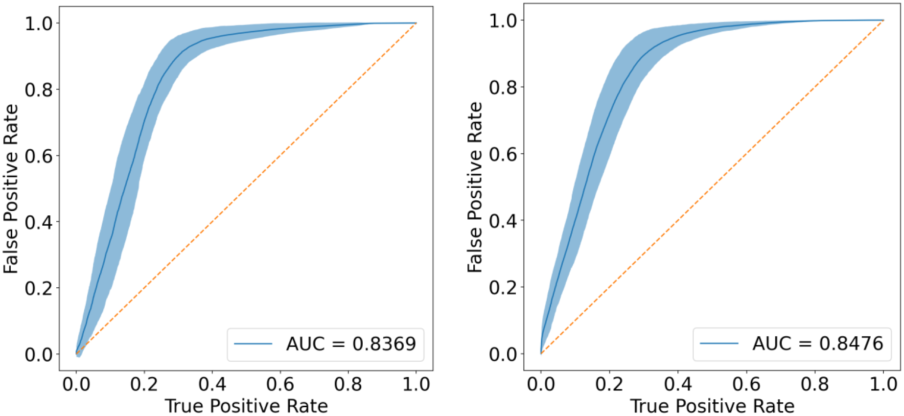
Receiver operating characteristic curves for manual (left) and automatic (right) selection with the ResNet-50 convolutional neural network. Of note, AUROC was slightly better with automatic selection (0.8476) but still very close in value with manual selection (0.8369). Another point of interest, ResNet-50 tended to show less variance than VGG19 and VGG16.
Figure 10.
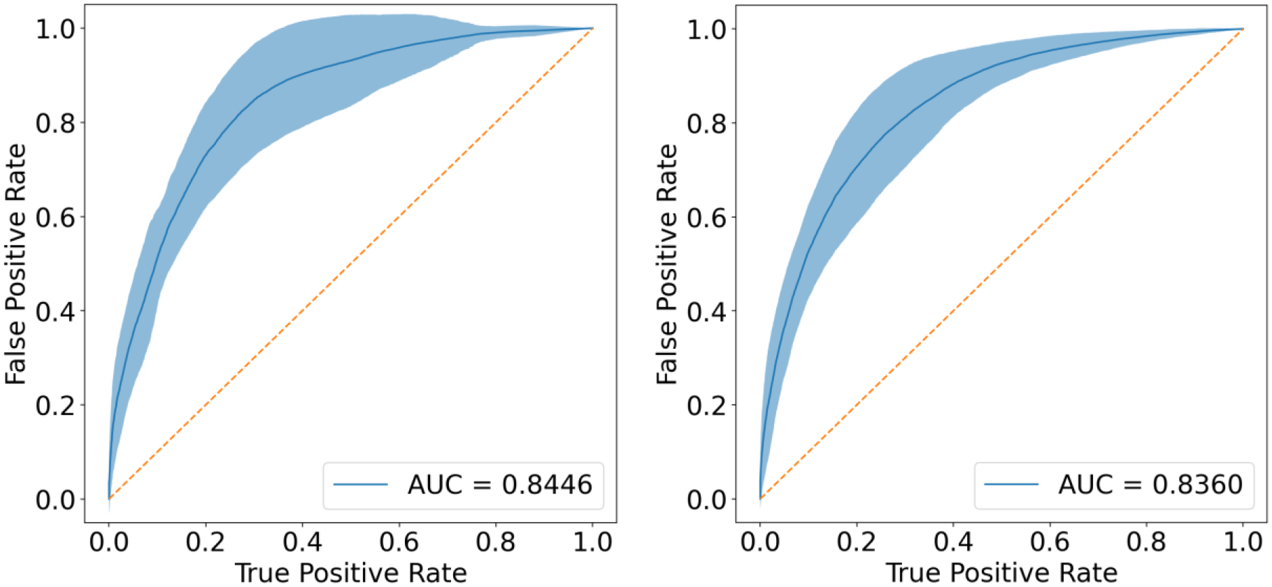
Receiver Operating Characteristic Curves for Manual (left) and Automatic (right) Selection with the VGG19 convolutional neural network.
Figure 11.
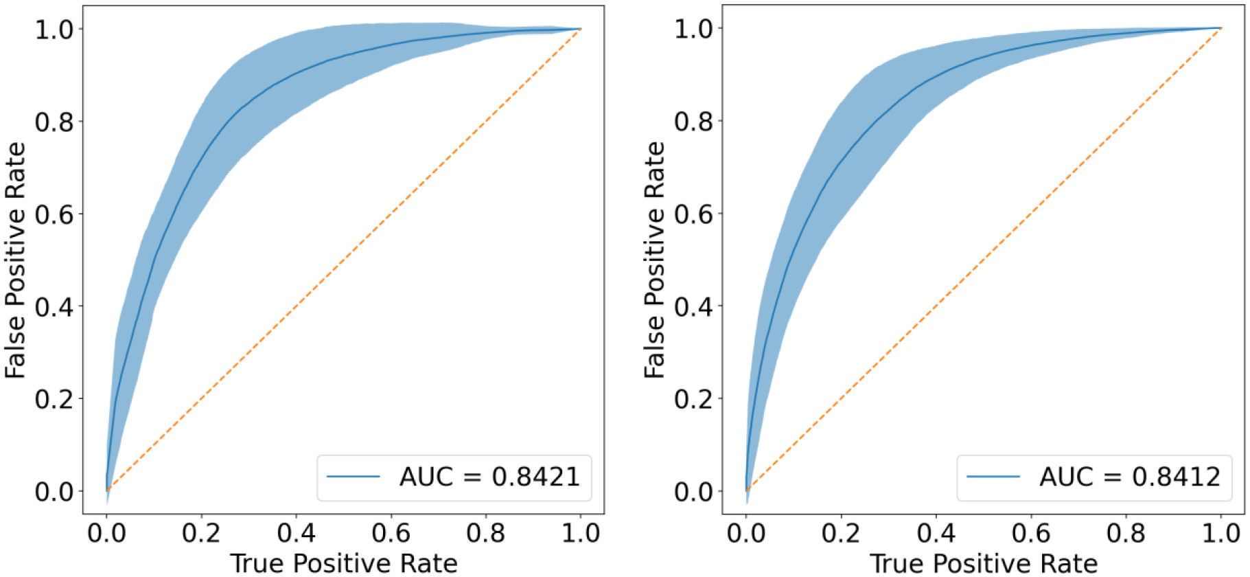
Receiver Operating Characteristic Curves for Manual (left) and Automatic (right) Selection with the VGG16 convolutional neural network.
5. DISCUSSION
Here we are able to show that automatic image data selection from CMR scans is possible and effective. While the manual selection method somewhat outperforms the automatic selection method, we believe that the automatic selection method has a lot of room to grow and should be able to match or exceed manual selection in the future.
We have also shown that using machine learning as a preprocessing step is an effect way to leverage the power of machine learning even before applying it for processing. While it is broadly understood that machine learning can be applied to many problems, the dual usage in both preprocessing and processing is something we believe could and should be applicable more widely for medical imaging data.
Further, we continue to validate that detection of IMS in CMR scans is possible and provides accuracy at around 80%. There are many exciting preprocessing methods we could still try and we believe that with further preprocessing, accuracy will improve.
Resources were limited when constructing the model architecture and running the classification. Video memory was limited to 8GB for this project. With greater resources available, it may be possible to construct and run more effective machine learning implementations to improve performance metrics.
While running the training process of the machine learning, we noticed some strong points of variability between different subsets of the dataset. This caused accuracy to fluctuate broadly at points with the average remaining close to 80%. This highlights the limitations of the particular size and composition of the dataset. In order to gain more widely applicable results and to further improve performance metrics and their stability, it will be necessary to apply this method to a larger and more balanced dataset.
6. CONCLUSIONS
The results of this work shows that it is possible to use machine learning not only to differentiate between patients with and without ischemic myocardial scarring, but also to streamline and automate the process of preparing image data for processing with machine learning. This is a promising application of machine learning diagnosis and represents, what will hopefully be, a strong stride forward as machine learning advances toward inclusion into clinical workflow.
ACKNOWLEDGEMENTS
This work was supported by NIH/NHLBI (K08HL131987, R01HL152090, and 1R01HL150266).
REFERENCES
- [1].Virani SS, Alonso A, Aparicio HJ, Benjamin EJ, Bittencourt MS, Callaway CW, … Tsao CW (2021). Heart Disease and Stroke Statistics-2021 Update: A Report From the American Heart Association. Circulation, 143(8), e254–e743. doi: 10.1161/cir.0000000000000950 [DOI] [PubMed] [Google Scholar]
- [2].Sharma UC, Zhao K, Mentkowski K, Sonkawade SD, Karthikeyan B, Lang JK, & Ying L (2021). Modified GAN Augmentation Algorithms for the MRI-Classification of Myocardial Scar Tissue in Ischemic Cardiomyopathy. Frontiers in cardiovascular medicine, 8, 726943–726943. doi: 10.3389/fcvm.2021.726943 [DOI] [PMC free article] [PubMed] [Google Scholar]
- [3].Torlasco C, Papetti D, Mene R, Artico J, Seraphim A, Badano L, … Nobile M (2021). Dark blood ischemic LGE segmentation using a deep learning approach. European Heart Journal - Cardiovascular Imaging, 22(Supplement_2). doi: 10.1093/ehjci/jeab090.020 [DOI] [Google Scholar]
- [4].O’Brien H, Whitaker J, Singh Sidhu B, Gould J, Kurzendorfer T, O’Neill MD, … Niederer S (2021). Automated Left Ventricle Ischemic Scar Detection in CT Using Deep Neural Networks. Frontiers in Cardiovascular Medicine, 8. doi: 10.3389/fcvm.2021.655252 [DOI] [PMC free article] [PubMed] [Google Scholar]
- [5].Gumpfer N, Grün D, Hannig J, Keller T, & Guckert M (2021). Detecting myocardial scar using electrocardiogram data and deep neural networks. Biological Chemistry, 402(8), 911–923. doi: 10.1515/hsz-2020-0169 [DOI] [PubMed] [Google Scholar]
- [6].Mason D (2011). SU-E-T-33: pydicom: an open source DICOM library. Medical Physics, 38(6Part10), 3493–3493. [Google Scholar]
- [7].Duda RO, & Hart PE (1972). Use of the Hough transformation to detect lines and curves in pictures. Communications of the ACM, 15(1), 11–15. [Google Scholar]
- [8].Bradski G (2000). The OpenCV Library. Dr. Dobb's Journal of Software Tools. [Google Scholar]
- [9].Clark A (2015). Pillow (PIL Fork) Documentation. readthedocs. Retrieved from https://buildmedia.readthedocs.org/media/pdf/pillow/latest/pillow.pdf
- [10].McMahan HB, Holt G, Sculley D, Young M, Ebner D, Grady J, … & Kubica J (2013, August). Ad click prediction: a view from the trenches. In Proceedings of the 19th ACM SIGKDD international conference on Knowledge discovery and data mining (pp. 1222–1230). [Google Scholar]
- [11].Pedregosa F, Varoquaux Ga”el, Gramfort A, Michel V, Thirion B, Grisel O, … others. (2011). Scikitlearn: Machine learning in Python. Journal of Machine Learning Research, 12(Oct), 2825–2830. [Google Scholar]


