Abstract
Medical image segmentation is a crucial step in Computer-Aided Diagnosis systems, where accurate segmentation is vital for perfect disease diagnoses. This paper proposes a multilevel thresholding technique for 2D and 3D medical image segmentation using Otsu and Kapur's entropy methods as fitness functions to determine the optimum threshold values. The proposed algorithm applies the hybridization concept between the recent Coronavirus Optimization Algorithm (COVIDOA) and Harris Hawks Optimization Algorithm (HHOA) to benefit from both algorithms' strengths and overcome their limitations. The improved performance of the proposed algorithm over COVIDOA and HHOA algorithms is demonstrated by solving 5 test problems from IEEE CEC 2019 benchmark problems. Medical image segmentation is tested using two groups of images, including 2D medical images and volumetric (3D) medical images, to demonstrate its superior performance. The utilized test images are from different modalities such as Magnetic Resonance Imaging (MRI), Computed Tomography (CT), and X-ray images. The proposed algorithm is compared with seven well-known metaheuristic algorithms, where the performance is evaluated using four different metrics, including the best fitness values, Peak Signal to Noise Ratio (PSNR), Structural Similarity Index (SSIM), and Normalized Correlation Coefficient (NCC). The experimental results demonstrate the superior performance of the proposed algorithm in terms of convergence to the global optimum and making a good balance between exploration and exploitation properties. Moreover, the quality of the segmented images using the proposed algorithm at different threshold levels is better than the other methods according to PSNR, SSIM, and NCC values. Additionally, the Wilcoxon rank-sum test is conducted to prove the statistical significance of the proposed algorithm.
Keywords: Image segmentation, Optimization, Thresholding, Hybrid algorithm
1. Introduction
Computer-Aided Diagnoses (CAD) tools play a critical role in healthcare [1]. Medical image segmentation is one of the essential steps for disease diagnoses. It refers to extracting objects of interest in medical images to analyze these objects' behavior, which may indicate the existence of a problem or a disease [2]. In the literature, several techniques have been proposed for image segmentation, such as edge detection-based segmentation [3], clustering-based segmentation [4], and thresholding-based segmentation [5]. Image segmentation based on thresholding is considered the most popular technique because it has simple implementation and high accuracy.
Despite the importance of image segmentation in extracting the objects of interest from medical images, some problems cause errors in the medical image segmentation process, such as image acquisition artifacts and corruption by noise. Various smoothing techniques can reduce error or remove noises, such as developing an algorithm or tuning a filter [6].
Depending on the number of thresholds used to segment the image, thresholding-based segmentation is classified into bi-level and multilevel thresholding [7]. In bi-level thresholding, one threshold is used to segment the image into two regions. All pixels with values more significant than the threshold value are classified as region 1, and the other pixels in the image are classified as region 2. On the other hand, multilevel thresholding involves using more than one threshold to segment the image into several regions. Bi-level thresholding fails to correctly identify images containing many objects with colored and complex backgrounds because it divides the image into only two classes. In such cases, multilevel thresholding is more appropriate [8]. The most critical step in the thresholding process is to find the optimum threshold values that efficiently determine the image segments. Over the last few decades, several strategies have been developed for determining the optimal thresholds; Ostu [9] and Kapur [10] methods are the most popular due to their efficiency and simplicity. Otsu's method maximizes the variance between classes, and Kapur's method maximizes the histogram entropy to measure homogeneity between segmented regions.
Image segmentation can be considered an optimization problem in which the objective is to find the optimum thresholds that precisely determine image classes. Traditional thresholding-based image segmentation techniques suffer from several problems, such as exponentially increasing the computational cost with the increase in thresholding levels which makes these methods suitable only for a small number of thresholding levels. This challenge encouraged the authors to use metaheuristics-based image segmentation algorithms as an alternative to the classical methods. Over the last years, several metaheuristic algorithms have been applied to solve image segmentation problems [11]. For multilevel thresholding, several algorithms have been used, such as the Genetic Algorithm (GA) [12], which is based on the theory of natural evolution; Particle Swarm Optimization (PSO) [13], inspired by the behavior of bird flocks and schooling fish; Artificial Bee Colony (ABC) [14] that simulates the behavior of bees in finding food sources; Harmony Search (HS) [15] inspired in musicians improvising new harmonies while playing; Electromagnetism Optimization (EO) [16] that mimics the attraction-repulsion mechanism among charges; and many others [[17], [18], [19], [20], [21], [22], [23], [24], [25], [26], [27]].
Several algorithms have been proposed for medical image segmentation, such as Harris Hawks' optimization algorithm, which is used to segment brain MRI images [28,28a]. The results showed that the proposed framework outperforms the state-of-the-art methods on the same dataset; however, it suffers from some limitations. It consumes more time than other metaheuristics. Another algorithm is proposed for COVID X-ray image segmentation using ant colony optimization with Cauchy and greedy levy mutations [29]. The results demonstrate the superior performance of the proposed algorithm in terms of search ability and convergence speed. Also, ABD ELAZIZ et al. [30,30a] proposed an algorithm for COVID-19 CT image segmentation based on an improved marine predators algorithm with fuzzy entropy. The experimental results approved the superiority of the proposed algorithm over the existing methods. The recently proposed metaheuristics that are used for solving multilevel thresholding image segmentation problems include the Arithmetic Optimization Algorithm (AOA) [31], which is inspired by the distribution behavior of the main arithmetic operators in mathematics, Remora Optimization Algorithm (ROA) [32] which mimics the parasitic behavior of remora, Black Window Optimization algorithm (BWO) [33], and Equilibrium Optimization Algorithm (EOA) [34]. These algorithms have proved their good performance; however, they may have limitations, such as getting stuck into local optima [35]. Some researchers employ hybridization as a way to avoid these limitations.
In image segmentation, many hybrid optimization algorithms have been proposed. For example, the Grasshopper Optimization Algorithm (GOA) is combined with the Differential Evolution algorithm (DE) for multilevel segmentation of satellite images [36]. The experimental results indicate that the proposed algorithm outperforms the standard GOA and DE algorithms. Also, a combination of the Gravitational Search Algorithm (GSA) and Genetic Algorithm (GA) is proposed for multilevel thresholding image segmentation using entropy and between-class variance as fitness functions [37]. The experimental results showed that the GSA-GA produced superior or comparative segmentation accuracy in entropy and between-class variance criteria. Many other hybrid algorithms are proposed to solve the image segmentation problem [38,39].
This paper proposes a novel hybrid optimization algorithm for multilevel thresholding 2D and 3D medical image segmentation based on combining the novel Coronavirus Disease Optimization Algorithm (COVIDOA) [40] and the Harris Hawks Optimization Algorithm (HHOA) [35]. COVIDOA is a recent evolutionary optimization algorithm that mimics the replication lifecycle of Coronavirus. COVIDOA has three main phases: Virus Entry, Virus Replication, and Virus mutation. Coronavirus uses frameshifting [41,42] to make new virus copies in the Replication phase. Frameshifting produces many viral proteins combined to form new virus particles as many new particles are created, and many human cells are damaged. In addition, the virus uses mutation techniques to escape from the human immunity system. COVIDOA has been applied to many benchmark test functions and real-world problems and showed superior performance. Its advantages include a good balance between exploration and exploitation and high convergence speed.
HHOA algorithm is a novel metaheuristic that mimics the chasing behavior of Harris hawks. HHOA has been applied to solve many real-world problems such as pressure vessel design problems, 3three-bar truss design problems, and welded beam design problems. HHOA shows good exploitative search ability.
This paper proposes combining COVIDOA and HHOA to find the optimum threshold values using Otsu's and Kapur's entropy as fitness functions. This hybridization helps benefit from both algorithms' advantages and overcome their limitations.
The reasons for using hybrid COVID and HHOA are as follows:
-
1.
The No Free Lunch (NFL) theorem demonstrates that no single algorithm performs best for all optimization problems. This theorem encouraged the authors to use a hybrid version of the recent COVIDOA to solve the image segmentation problem.
-
2.
The COVIDOA [40] and its binary version, BCOVIDOA [43], outperformed most existing optimization algorithms in solving benchmark and real-world optimization problems.
-
3.
The idea of the proposed algorithm is to divide the initial population into two half and assign each half to one of the two powerful metaheuristics (COVIDOA and HHOA). The two metaheuristics then work in parallel to update the two half populations. Then the updated two subpopulations are merged into one full population. These stapes are repeated until the maximum number of iterations is reached and finally output the optimum solution found so far. The idea of the proposed algorithm is very simple and can be easily implemented.
-
4.
The proposed approach makes parallel hybridization (which is more suited to parallel computer environments) between two powerful metaheuristics (COVIDOA and HHOA) for solving segmentation problems.
-
5.
The proposed algorithm can fix the limitations of the two metaheuristics because each technique operates on only half of the population, not the whole population.
-
6.
Traditional thresholding-based image segmentation techniques suffer from several problems, such as exponentially increasing the computational cost, which encouraged the authors to use metaheuristics-based image segmentation algorithms as an alternative to the classical methods. Our proposed algorithm achieved superior performance in medical image segmentation, especially at high thresholding levels in which traditional methods are unsuitable due to the high computational cost.
-
7.
The proposed hybrid technique can be easily applied to any other metaheuristics. Still, we preferred combining COVIDOA and HHOA algorithms because of their superior performance in solving various optimization problems.
The proposed algorithm works as follows: the population of solutions is divided into two halves, and then each half is assigned to one of the two algorithms. Each algorithm operates in parallel with its sub-population and generates the updated sub-population. The two generated sub-populations are combined to form one new population in which the optimum solution is found. The validity of the proposed algorithm in solving various optimization problems is proved by solving 6 test problems from IEEE CEC 2019 benchmark problems [44]. In Medical image segmentation, the quality of the segmented medical images using the proposed algorithm is evaluated using different metrics such as MSE, PSNR, SSIM, FSIM, and NCC. The proposed algorithm is compared with seven state-of-the-art metaheuristics such as Harris Hawks Optimization Algorithm (HHOA) [35], Bat Algorithm (BA) [23], Harmony Search Algorithm (HS) [15], Cuckoo Search Algorithm (CS) [19], Sine Cosine Algorithm (SCA) [22], Flower Pollination Algorithm (FPA) [18], and Seagull Optimization Algorithm (SOA) [45]. In addition, the Wilcoxon rand sum test is calculated to prove the statistical significance of the proposed algorithm.
The main contributions of this paper can be summarized as follows:
-
•
A novel hybrid COVIDOA-HHOA algorithm is proposed for medical image segmentation.
-
•
The efficiency of COVIDOA-HHOA is demonstrated by solving six IEEE CEC 2019 problems.
-
•
The performance of COVIDOA-HHOA is compared with seven well-known metaheuristics.
-
•
The comparison proved the superior performance of COVIDOA-HHOA against its beers.
-
•
Two datasets are used for testing, including 2D and 3D medical images.
-
•
Best fitness, PSNR, SSIM, and NCC metrics evaluate performance.
-
•
The Wilcoxon rank-sum test is conducted to prove the efficiency of COVIDOA-HHOA.
This paper is organized as follows: Section 2 provides a brief overview of multilevel thresholding techniques such as Otsu's method and Kapur's entropy. Sections 3, 4 give an overview of Coronavirus disease optimization and Harris hawks optimization, respectively. The proposed hybrid algorithm for multilevel thresholding is discussed in Section 5. The medical datasets, parameter setting, performance metrics, and experimental results are discussed in Section 6. Finally, conclusions and future work are given in Section 7.
2. Multilevel thresholding
Image thresholding is converting the color or gray scale image into a binary image by setting a threshold value on the pixel intensity of the image [46]. Where pixels below that threshold value are converted to black and pixels above it are converted to white. Image thresholding can be categorized into two classes: bi-level and multilevel. Bi-level thresholding aims to assign each pixel p of a graey-scale image to one of two regions (R1 and R2) using only one threshold value (th) as follows:
| (1) |
where refers to maximum intensity level.
However, multilevel thresholding segments an image into several distinct regions using more than one threshold value as follows:
| (2) |
where {} represents a vector of different threshold values.
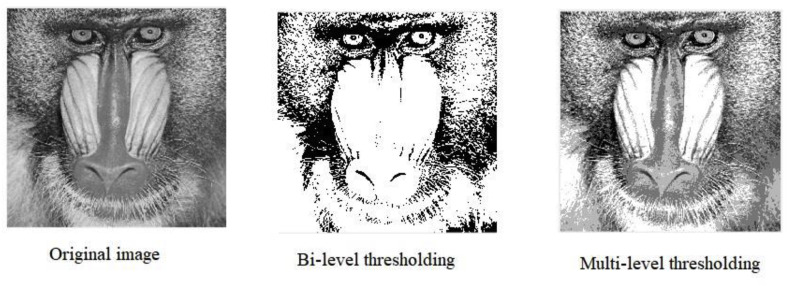
Fig. 1 shows the difference between bi-level thresholding and multilevel thresholding of the mandrill baboon image.
Fig. 1.
Bi-level and multilevel thresholding.
The optimal threshold values can be obtained by maximizing a fitness function. Otsu's method and Kapur's entropy are two popular techniques used in thresholding. Each technique proposes a different fitness function that must be maximized to obtain the optimal threshold values. The two techniques are briefly described in the following subsections.
2.1. Otsu's method
Otsu is a thresholding method that selects the optimal threshold by maximizing the variance value between different classes [9]. Assume that we have L intensity levels in a gray scale image, where L=256 and a vector V of k-1 thresholds are used to segment the image into k regions as in equation (2), where V = [th 1 , th 2 , …, th k-1 ]. Then the best threshold is obtained by maximizing the Otsu's fitness function as follows:
| (3) |
where V=[th 1 , th 2 , …, th k-1 ], and represents the between-class variance which can be expressed as follows:
| (4) |
where is the cumulative probability for region R k, is the average intensity in region R k and is the average intensity for the whole image as follows:
| (5) |
where is the probability of gray level i, which can be represented as follows:
| (6) |
where fi is the frequency of gray level i.
2.2. Kapur's entropy method
Image entropy represents the compactness and separateness between image classes [10]. The Kapur method is another widely used thresholding method that aims to find the optimal threshold value by maximizing the Kapur's entropy as follows:
| (7) |
where
where is described in Eq. (6).
For muli-level thresholding, Kapur's method can be defined as follows:
| (8) |
The symbol V is the vector of thresholds.
3. Coronavirus Disease Optimization Algorithm
COVIDOA is a recently proposed population-based optimization algorithm that simulates the replication mechanism of Coronavirus when getting inside the human body [40]. The replication process of Coronavirus has four main stages as follows:
-
1.
Virus entry and uncoating
When a human is infected with COVID, the Coronavirus particles attach to the human cell via one of its structural proteins, called spike protein [42]. After getting inside the human cell, the virus contents are released.
-
2.
Virus replication
The virus's replication technique is called the frameshifting technique [41]. Frameshifting is moving the reading frame of a protein sequence of the virus to another reading frame that leads to the creation of many new viral proteins that are then merged to form new virus particles. There are many types of frameshifting techniques; however, the most popular is +1 frameshifting as follows:
-
•
+1 frameshifting technique
The elements of the parent virus particle (parent solution) are moved in the right direction by 1 step. As a result of +1 frameshifting, the first element is lost. In the proposed algorithm, the first element is set as a random value in the range [, Ub] as follows:
| (9) |
| (10) |
where and are the lower and upper bounds for the variables in each solution.
-
3.
Virus mutation
Coronavirus uses mutation to resist the human immune system [47]. In the proposed algorithm, the mutation is applied to the previously created new virus particle (solution) to produce a new one as follows:
| (11) |
The symbol X referes to the solution before mutation, Z is the mutated solution, X i and Z i are the ith element in the old and new solutions, respectively, i = 1, …, D, and r is a random value in the range [, ], MR is the mutation rate.
-
4.
New virion release
The newly created virus particle leaves the infected cell targeting new healthy cells. In the proposed algorithm, if the fitness of the new solution is better than the parent solution fitness, the parent solution is replaced by the new one. Otherwise, the parent solution remains.
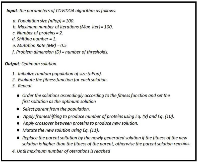
The pseudocode of the COVID optimization algorithm is shown in Fig. 2 .
Fig. 2.
pseudocode of COVID optimization algorithm.
4. Harris hawks optimization
HHOA [35] is a population-based algorithm inspired by the chasing behavior of Harris hawks to capture prey. The two main phases of HHOA are exploration and exploitation, which are explained in the following subsections.
4.1. Exploration
In this phase, The Harris Hawks update their position based on two strategies with equal chance P. If p < 0.5, the position is updated based on the position of another family member. If p > 0.5, the Harris Hawks perch on random tall trees and wait to find prey. These two strategies are modeled in equation (1).
| (12) |
where is the position of a hawk in the next iteration, is the position of hawk of the current iteration, is a randomly selected hawk from the current population, is the position of the intended prey, , , , and are random numbers in the range [0,1]. Lb and Ub are the lower and upper bounds, is the average position vector of all hawks in the population, which can be calculated as follows:
| (13) |
where N is the total number of hawks in the population, t refers to the current iteration, represents the position of the ith hawk in the population.
4.2. The transition from exploration to exploitation
While the prey is escaping from the attack, its energy continuously decreases. The energy can be modeled as follows:
| (14) |
where E refers to the escaping energy of the prey at each iteration. is the initial energy of the prey, which varies between −1 and 1, and T is the maximum number of iterations. When , the algorithm is in the exploration phase, where the hawks explore different regions. In contrast, when , the algorithm is in the exploitation phase.
4.3. Exploitation phase
The exploitation phase can be modeled based on the prey's ability to escape from being hunted and the chasing approaches of the Hawks. If a random number r is less than 0.5, the rabbit has successfully run away. Otherwise, the rabbit failed to escape. On the other hand, the behavior of Harris Hawks depends on the prey's escaping energy E. If , the Hawks perform soft besiege; otherwise, they perform hard to besiege. Four stages are considered to simulate this phase, as follows:
4.4. Soft besiege
This stage simulated the case in which the rabbit failed to escape from attack (), although it had enough energy (). In this case, the Hawks update their location according to the following equations:
| (15) |
The refers to the difference between the rabbit's position and the hawk's current location at iteration t. The J represents the power of the prey's jump while escaping. Finally, is a random number in the range [0, 1].
4.5. Hard besiege
The Hawks perform hard besiege when and means that the prey becomes very tired and has not enough energy to escape. This case can be modeled as follows:
| (16) |
4.6. Soft besiege with progressive rapid dives
In this case, and which means that the prey has enough energy to escape, and the Hawks perform soft besiege and find their next position by the following equation:
| (17) |
If the position is not improved, team rapid dives based on levy flight will be executed as follows:
| (18) |
where S is a randomly selected vector of dimension D. LF represents the levy flight function and can be calculated as follows:
This stage can be summarized as follows:
| (19) |
4.7. Hard besiege with progressive rapid dives
In this case, and which means that the prey does not have enough energy to escape, and a hard besiege is executed by the Hawks as follows:
| (20) |
where
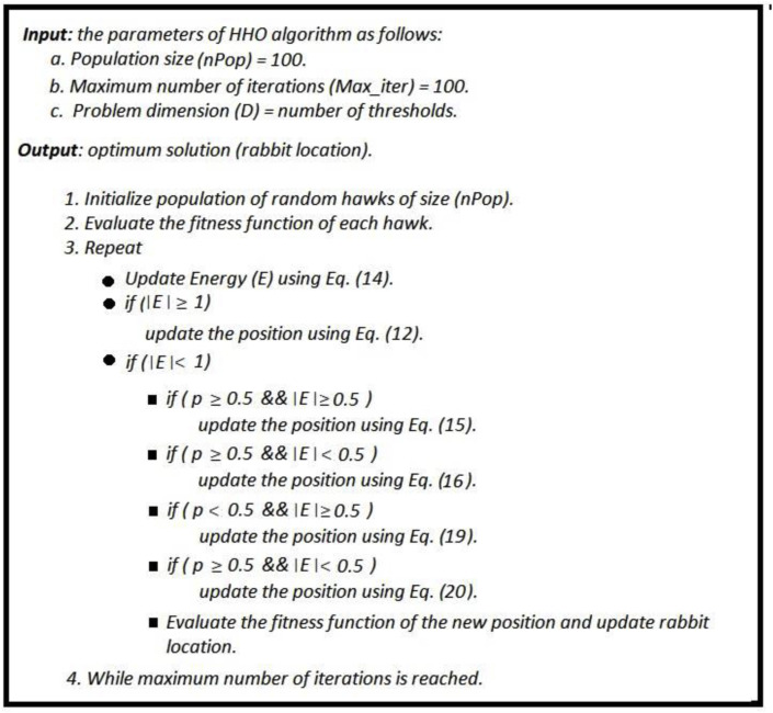
The is the mean location defined in equation (13). The pseudocode of the HHOA algorithm is shown in Fig. 3 .
Fig. 3.
Pseudocode of HHOA algorithm.
5. The proposed hybrid algorithm (COVID-HO)
Because of some limitations in each metaheuristic, researchers tend to use a hybridization strategy to improve the performance and overcome these limitations. According to the execution order, metaheuristic hybridization is classified into sequential and parallel [48]. In Sequential hybridization, the output of the first algorithm is used as input to the second. On the other side, parallel hybridization approaches similarly apply the algorithms. Although most of the proposed hybrid metaheuristics are sequential, researchers of these sequential metaheuristics indicate the parallelization of their algorithms as future work because parallel hybrid metaheuristics are more suited to parallel computer environments [49].
Although HHOA and COVID algorithms effectively solve various engineering problems, each one separately can suffer from limitations such as falling into local optimum in HHOA and being time-consuming in COVID. This paper combines the two algorithms to produce a parallel hybrid COVID-HHOA algorithm to minimize the drawbacks of both algorithms and benefit from their advantages. It then solves the thresholding problem using Otsu's method and Kapur's entropy as objective functions.
The proposed hybrid algorithm can be summarized as follows:
-
1.
The population of solutions of size nPop is randomly initialized.
-
2.
The fitness function is calculated for each solution, and the solution with the best fitness is set as the rabbit location.
-
3.
The population is divided into two sub-populations such that solutions from 1 to The initial population is considered the first sub-population, and the remaining solutions are considered the second subpopulation.
-
4.
The first sub-population is assigned to the COVID algorithm, and the second subpopulation is assigned to the HHOA algorithm.
-
5.
The two algorithms operate in parallel to produce two updated sub-populations.
-
6.
The two new sub-populations are combined into one population.
-
7.
Steps 2–6 are repeated until the maximum number of iterations is reached.
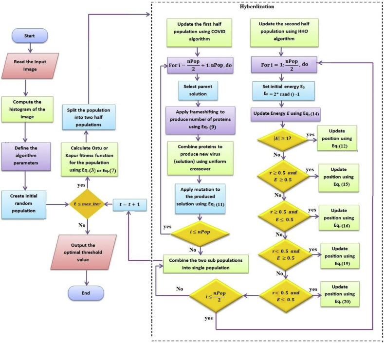
The flow chart of the proposed COVID-HHOA algorithm for multi-thresholding segmentation for 2D images is shown in Fig. 4 .
Fig. 4.
Flowchart of the proposed COVID- HHOA algorithm.
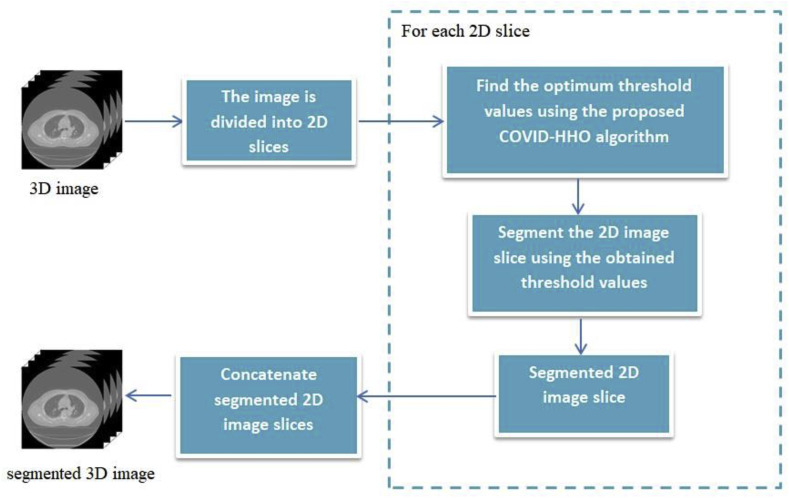
In the case of 3D medical images, the image is divided into several 2D slices, and each slice is segmented using the proposed algorithm. The segmented slices are concatenated together to form the segmented 3D image, as shown in Fig. 5 .
Fig. 5.
Diagram of multilevel thresholding image segmentation for 3D images using the proposed COVID-HHOA algorithm.
The advantages of medical image segmentation using our proposed approach are as follows:
-
1.
Segmentation has a crucial role in medical imaging as it helps to separate the objects of interest from the whole body, simplifying medical decisions.
-
2.
The segmentation approach, which gives perfect results for one type of imaging modality, might not even work for another. Our proposed approach achieved very good segmentation results for several medical images from different modalities (CT, MRI, and X-ray).
-
3.
The proposed approach makes parallel hybridization (which is more suited to parallel computer environments) between two powerful metaheuristics (COVIDOA and HHOA) for solving segmentation problems.
-
4.
It can be applied to any two population-based metaheuristics.
-
5.
Its computational time is half the computational time of sequential hybrid metaheuristics because the initial population is divided into two halves, and each algorithm operates on one half in parallel.
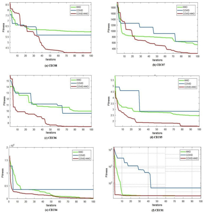
To prove the superiority of the proposed Hybrid COVID-HHOA algorithm over the native HHOA and COIVD algorithms, we utilized 6 test functions from IEEE CEC 2019 benchmark problems. These are a group of modern test functions known as “The 100-Digit Challenge” intended to be used in single objective numerical optimization IEEE competitions. The description of these functions in terms of problem dimension, range of possible values, and the global optimum is discussed in Ref. [50].
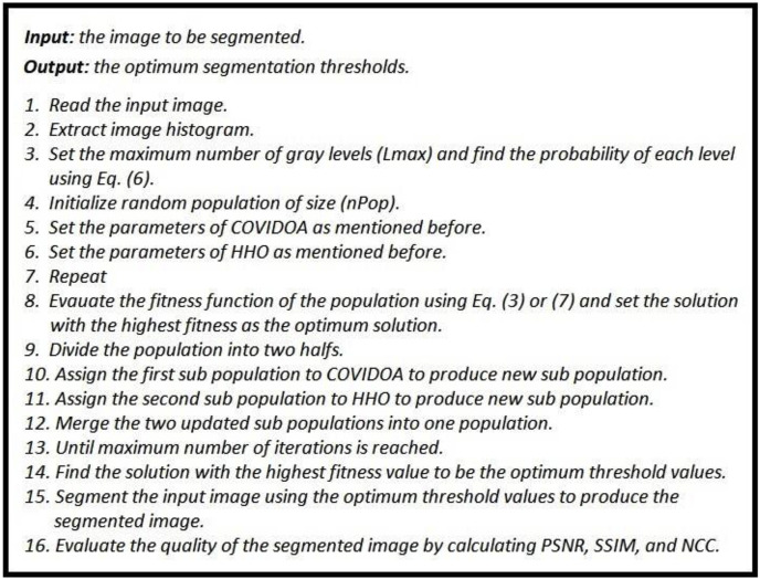
The convergence curves of the proposed hybrid algorithm, HHOA, and COVID algorithms are presented in Fig. 6 . The figure clearly shows the superiority of the proposed hybrid algorithm as it reaches the optimum fitness values compared to COVID and HHOA algorithms. The pseudocode of the proposed COVID-HHOA algorithm for multilevel thresholding is shown in Fig. 7 .
Fig. 6.
Comparison of convergence curves of hybrid COVID-HHOA, HHOA, and COVID algorithms using CEC 2019 test problems.4.
Fig. 7.
Pseudocode of the proposed COVID_HHOA optimization algorithm for multilevel thresholding.
6. Experimental results and discussion
In this section, we firstly provide a brief description of the medical datasets used for testing. Then, we show the parameter settings for the proposed and state-of-the-art algorithms. After that, the evaluation metrics used for comparing the results are explained in detail. Then, we present the numerical results obtained from running the proposed algorithm and its peers. Finally, we conducted a comparative analysis of the obtained results.
6.1. Datasets
6.1.1. 2D medical images
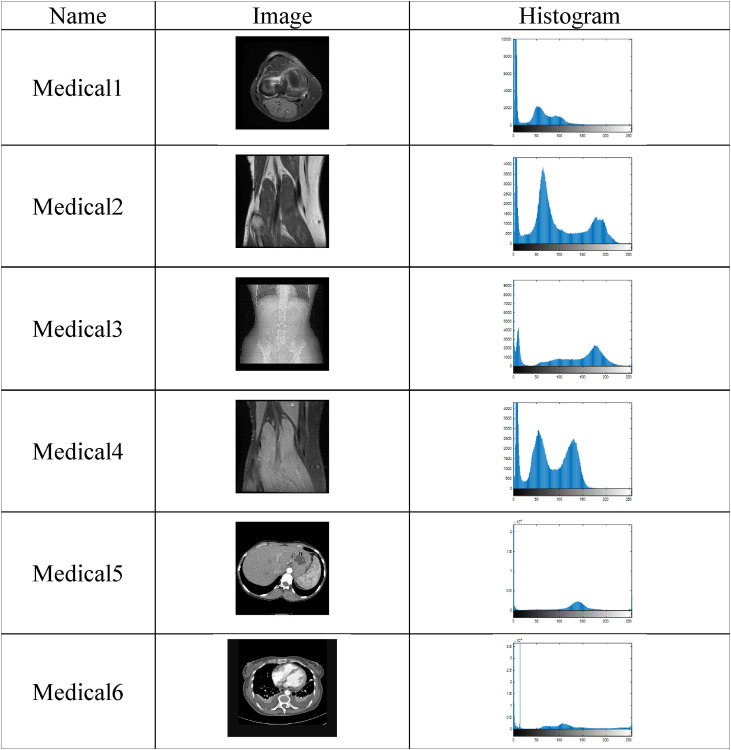
We used six 2D medical images to prove the efficiency of the proposed algorithm in medical image segmentation. Medical1, Medical2, and Medical4 images are MRI images, Medical3 are X-ray images, and Medical5 and Medical6 are CT images. These images have many variations, such as size, resolution, and modality. The images and their histograms are shown in Table 1 .
Table 1.
Test images and their histograms.
6.1.2. Volumetric (3D) medical images
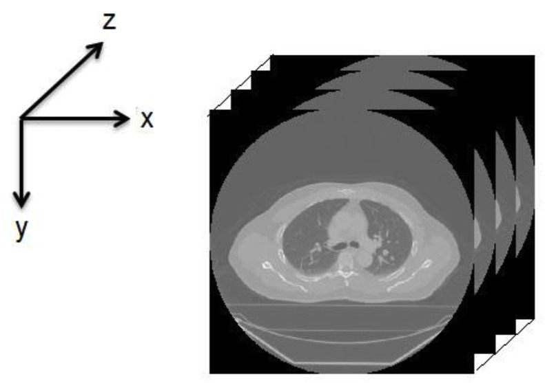
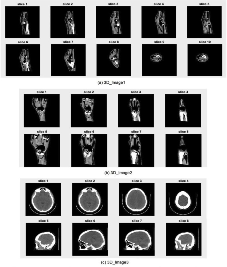
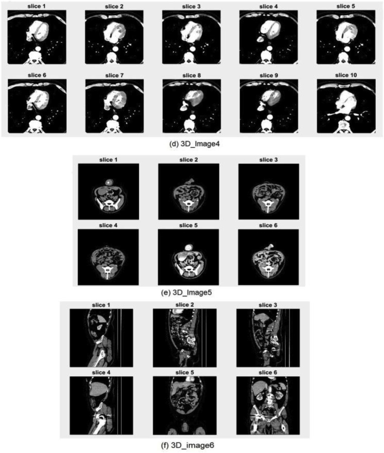
The advanced medical imaging technologies available today, such as MRI, CT, X-ray, and ultrasound, make it possible to view the detailed structure of human anatomy by acquiring efficient volumetric medical images. These images make it easier for medical experts to examine, detect, and diagnose diseases. Volumetric medical images can be represented by a group of 2D image slices [51], as shown in Fig. 8 . A set of 3D medical images are selected for testing from the open-source dataset available in Ref. [52]. The selected image slices are shown in Fig. 9 .
Fig. 8.
3D (volumetric) medical image.
Fig. 9.
Original volumetric medical images used for testing.
6.2. Parameter setting
The results of multilevel thresholding using the proposed algorithm are compared with those of seven well-known metaheuristic algorithms in different evaluation criteria. These algorithms are: Harris Hawks Optimization Algorithm (HHOA) [35], Bat Algorithm (BA) [23], Harmony Search Algorithm (HSA) [15], Cuckoo Search Algorithm (CSA) [19], Sine Cosine Algorithm (SCA) [22], Flower Pollination Algorithm (FPA) [18], and Seagull Optimization Algorithm (SOA) [45].
The reasons for selecting these algorithms for comparison are as follows:
-
⁃
They have proved their superior performance in solving various optimization problems, especially image segmentation.
-
⁃
Most of them are recent and published in reputable sources.
-
⁃
Their MATLAB implementations are publicly available on the MATLAB website (https://www.mathworks.com/).
All the experiments were run on a laptop with the following specifications: Intel(R) Core(TM) i7-1065G7 processor, RAM of 8.0 GB size, and Windows 10 Ultimate 64-bit operating system. All the algorithms are developed using MATLAB R2016a development environment.
6.3. Performance metrics
The performance of the proposed algorithm is evaluated using several performance metrics, including Peak Signal-to-Noise Ratio (PSNR), Structural Similarity Index (SSIM), Normalized Correlation Coefficient (NCC), and best fitness, in addition to the Wilcoxon rank-sum test.
PSNR, SSIM, and NCC are used to measure the quality of the segmented images, while best fitness is measured to prove the ability of the proposed algorithm to find optimum solutions, and the Wilcoxon rank-sum test is utilized to prove the statistical significance of the proposed algorithm as follows:
-
a)
Best Fitness
The maximum fitness obtained from running the proposed ad state-of-the-art algorithms with Otsu's method and Kapur's entropy functions is measured using equations (3), (7).
-
b)
Peak signal-to-noise ratio (PSNR)
PSNR is commonly used to quantify the quality of images. It refers to the ratio between the segmented image power and noise power. PSNR for 2D and 3D images is calculated as follows:
| (21) |
where of a 2D image is calculated as follows:
| (22a) |
F(i,j) is the original image, f(i,j) is the segmented image, and refers to the 2D image size.
For 3D images, the MSE is calculated as follows:
| (22b) |
where F(i,j,k) is the original 3D image, f(i,j,k) is the segmented 3D image, and refers to the size of the 3D image.
-
c)
Structural similarity index (SSIM)
SSIM is used to quantify the structural similarity between the original and segmented images; the SSIM for 2D and 3D images is calculated as follows:
| (23) |
The F and f refer to the original and segmented images. The and are the mean intensity of F and f, while and refer to the variance of F and f, respectively. The values of C 1 = 6.502 and C2 = 58.522 are used.
-
d)
Normalized correlation coefficient (NCC)
NCC is used to measure the extent to which two images are related. The absolute value of NCC ranges from 0 to 1, where 0 indicates that the two images have no relation and 1 indicates the strongest possible relation. The higher the absolute value of NCC, the stronger the relationship between the two images.
NCC between the original and segmented 2D images F(i,j) and f(i,j) is calculated as follows:
| (24) |
where is the size of the 2D image.
The NCC between two 3D images F(i,j,k) and f(i,j,k) is calculated as follows:
-
e)
Wilcoxon rank-sum test
The Wilcoxon rank-sum test is a non-parametric statistical test used to measure the statistical difference between two related methods [51]. We conducted the Wilcoxon rank-sum test with a 5% significance level to prove the proposed algorithm's statistical significance compared to the other algorithms.
6.4. Results
This section presents the numerical results of running the proposed algorithm to select the optimum threshold values using Otsu's method and Kapur's Entropy. These results are compared with the state-of-the-art algorithms regarding best fitness, PSNR, SSIM, NCC, and Wilcoxon rank-sum test. This section is divided into two subsections for presenting the results of using the proposed algorithm to segment 2D and 3D medical images as follows:
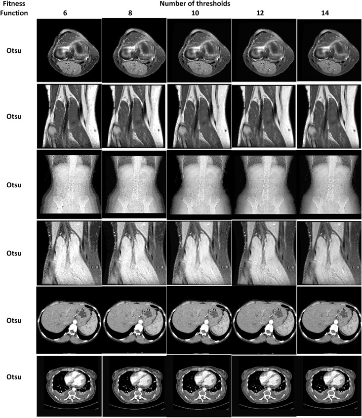
6.4.1. Experimental results for 2D medical images
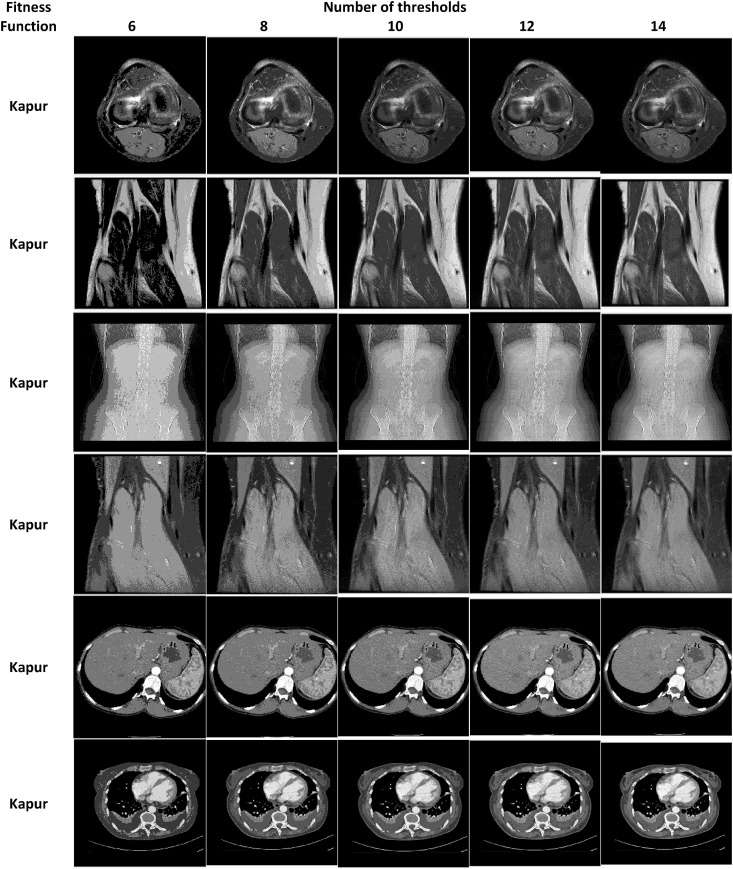
Table 2, Table 3 show the segmentation results of the 2D medical test images using the proposed COVID-HHOA algorithm. These images are segmented using Otsu's method and Kaur's Entropy fitness functions at 6, 8, 10, 12, and 14 threshold levels.
Table 2.
Medical Images segmented by the proposed COVID-HHOA algorithm using Otsu's method.
Table 3.
Medical Images segmented by the proposed COVID-HHOA algorithm using Kapur's entropy method.
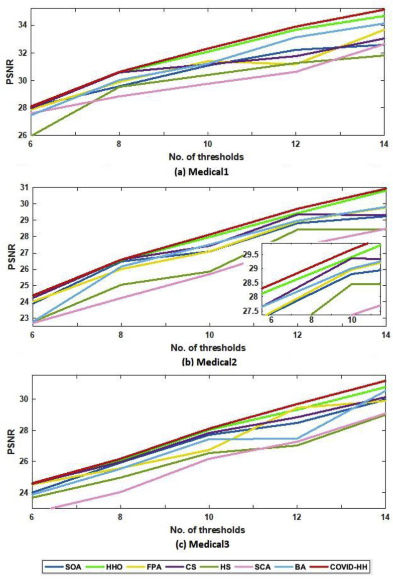
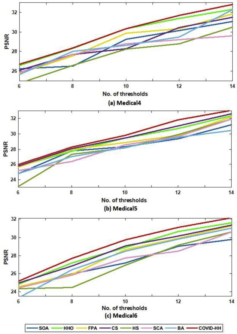
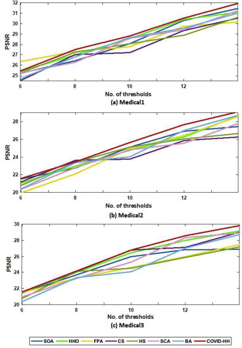
Table 4, Table 5 show the PSNR values produced by the proposed and state-of-the-art algorithms for all test images using Otsu's method and Kapur's entropy at different threshold levels. It's shown from the tables that the proposed algorithm has the highest PSNR in 59 from 60 cases.
Table 4.
PSNR results of Otsu's method for all algorithms.
| Image | K | Algorithms |
|||||||
|---|---|---|---|---|---|---|---|---|---|
| SOA [45] | HHOA [35] | FPA [18] | CS [19] | HS [15] | SCA [22] | BA [23] | COVID-HHOA | ||
| Medical1 | 6 | 28.0241 | 28.0015 | 27.8603 | 27.9327 | 25.9398 | 27.6060 | 27.4521 | 28.1034 |
| 8 | 29.5159 | 30.5702 | 29.8950 | 30.5846 | 29.4844 | 28.8106 | 30.0270 | 30.6115 | |
| 10 | 31.0962 | 32.0855 | 31.4062 | 31.1762 | 30.3947 | 29.7557 | 31.2010 | 32.3208 | |
| 12 | 32.2296 | 33.6432 | 31.1533 | 31.7412 | 31.2790 | 30.6256 | 33.1004 | 33.8829 | |
| 14 | 32.5824 | 34.6792 | 33.6707 | 33.0175 | 31.8011 | 32.6048 | 34.0983 | 35.1157 | |
| Medical2 | 6 | 23.8976 | 24.3012 | 23.9940 | 24.2262 | 22.7669 | 22.6919 | 22.7570 | 24.3882 |
| 8 | 26.4672 | 26.5729 | 26.0080 | 26.5961 | 25.0116 | 24.2180 | 26.1634 | 26.6181 | |
| 10 | 27.0786 | 27.9677 | 27.0960 | 27.4578 | 25.8210 | 25.6833 | 27.5117 | 28.1228 | |
| 12 | 28.8093 | 29.4139 | 28.9450 | 29.3669 | 28.4395 | 27.3844 | 28.9853 | 29.6817 | |
| 14 | 29.2411 | 30.7983 | 29.7738 | 29.3305 | 28.4481 | 28.4797 | 29.8231 | 30.9323 | |
| Medical3 | 6 | 24.0112 | 24.5539 | 24.5079 | 24.5771 | 23.6808 | 22.7121 | 23.8876 | 24.5965 |
| 8 | 25.9225 | 26.0874 | 25.5731 | 25.9562 | 24.9593 | 24.0463 | 25.5063 | 26.1987 | |
| 10 | 27.7211 | 28.0173 | 26.7435 | 27.8348 | 26.5461 | 26.1655 | 27.4362 | 28.1225 | |
| 12 | 28.4870 | 29.2997 | 29.4472 | 28.8344 | 27.0262 | 27.2857 | 27.4541 | 29.6674 | |
| 14 | 29.9596 | 30.7411 | 29.8566 | 30.1048 | 28.9854 | 29.0777 | 30.5004 | 31.1412 | |
| Medical4 | 6 | 26.2450 | 26.5800 | 25.7530 | 26.0731 | 24.7475 | 25.8652 | 25.6488 | 26.6784 |
| 8 | 26.5107 | 28.3621 | 27.5579 | 27.7016 | 26.5912 | 27.6891 | 28.0003 | 28.4004 | |
| 10 | 29.2529 | 30.3418 | 29.8796 | 28.3021 | 28.2514 | 28.7927 | 28.6717 | 30.3635 | |
| 12 | 30.1704 | 31.3994 | 30.3462 | 30.4476 | 28.8059 | 29.2508 | 29.5124 | 31.6963 | |
| 14 | 31.0825 | 32.3168 | 31.8551 | 31.5092 | 30.4896 | 29.6222 | 32.2716 | 32.8176 | |
| Medical5 | 6 | 24.7579 | 25.7082 | 25.6246 | 25.7676 | 23.1043 | 25.1616 | 24.7941 | 25.9592 |
| 8 | 27.7621 | 27.7409 | 27.9747 | 28.0629 | 27.3604 | 26.3591 | 27.0363 | 28.2565 | |
| 10 | 28.3140 | 29.4341 | 28.8750 | 29.4337 | 28.1992 | 28.5822 | 28.2220 | 29.7908 | |
| 12 | 29.3404 | 30.7092 | 29.7841 | 31.0181 | 29.8806 | 29.6569 | 29.5604 | 31.8339 | |
| 14 | 31.1842 | 32.3781 | 32.2351 | 32.6095 | 31.9152 | 31.9355 | 30.4210 | 33.0516 | |
| Medical6 | 6 | 24.4866 | 24.8421 | 24.5311 | 24.9414 | 24.3269 | 24.4083 | 23.3405 | 25.1480 |
| 8 | 25.9630 | 27.2037 | 25.9113 | 26.8320 | 24.4700 | 25.8269 | 26.4225 | 27.6991 | |
| 10 | 27.2134 | 28.9124 | 28.6518 | 29.0542 | 26.9230 | 27.7604 | 28.4883 | 29.7148 | |
| 12 | 29.0199 | 30.6417 | 29.9051 | 30.1581 | 29.1440 | 28.4976 | 29.7973 | 31.1191 | |
| 14 | 29.7714 | 31.6065 | 31.2646 | 31.3577 | 30.5977 | 30.6166 | 31.0194 | 32.1560 | |
Table 5.
PSNR results of Kapur's entropy for all algorithms.
| Image | K | Algorithms |
|||||||
|---|---|---|---|---|---|---|---|---|---|
| SOA [45] | HHOA [35] | FPA [18] | CS [19] | HS [15] | SCA [22] | BA [23] | COVID-HHOA | ||
| Medical1 | 6 | 25.2524 | 25.4433 | 26.3512 | 24.5522 | 25.2684 | 25.2804 | 24.7321 | 25.4509 |
| 8 | 26.4326 | 26.9740 | 27.3109 | 27.0291 | 27.2530 | 26.2667 | 26.7912 | 27.5253 | |
| 10 | 28.0860 | 28.5479 | 27.7927 | 27.2030 | 28.0816 | 28.5909 | 28.6896 | 28.8268 | |
| 12 | 30.3107 | 30.4151 | 29.7459 | 29.3509 | 28.9154 | 29.4261 | 29.5701 | 30.5083 | |
| 14 | 31.4768 | 31.0771 | 30.1544 | 30.5344 | 30.5967 | 31.2580 | 31.0262 | 31.9442 | |
| Medical2 | 6 | 21.5328 | 21.0665 | 19.9647 | 21.1612 | 20.7791 | 20.3524 | 20.3740 | 21.5760 |
| 8 | 22.7437 | 22.9694 | 22.0828 | 23.6234 | 23.4112 | 22.8048 | 23.3296 | 23.4328 | |
| 10 | 25.1282 | 24.7891 | 24.9807 | 23.7998 | 25.1116 | 24.8474 | 24.0673 | 25.6612 | |
| 12 | 26.9097 | 26.2715 | 26.4183 | 25.8614 | 26.0482 | 25.5683 | 27.0147 | 27.6624 | |
| 14 | 27.4481 | 28.6800 | 28.5732 | 26.2504 | 26.6410 | 27.8178 | 28.7076 | 29.1074 | |
| Medical3 | 6 | 21.4500 | 21.5384 | 21.4728 | 21.5716 | 20.7611 | 21.1768 | 20.9559 | 21.5922 |
| 8 | 23.6874 | 24.0349 | 23.3270 | 24.1519 | 24.1593 | 23.7441 | 23.2662 | 24.1918 | |
| 10 | 25.9861 | 26.4415 | 24.6536 | 26.7867 | 24.5258 | 26.1975 | 25.3053 | 26.7991 | |
| 12 | 26.8566 | 28.0038 | 25.9627 | 27.1257 | 25.8697 | 26.9955 | 28.3338 | 28.5621 | |
| 14 | 26.8949 | 29.1298 | 27.4718 | 29.0164 | 27.2153 | 27.4595 | 28.8884 | 29.8025 | |
| Medical4 | 6 | 21.8727 | 22.1638 | 21.4247 | 21.0408 | 21.8694 | 21.5044 | 22.0440 | 22.3226 |
| 8 | 24.8756 | 24.4229 | 23.8503 | 23.4907 | 23.8887 | 24.3239 | 23.9722 | 24.9068 | |
| 10 | 25.8773 | 25.6581 | 24.4352 | 25.2046 | 25.9492 | 25.9190 | 24.7383 | 26.3789 | |
| 12 | 28.4434 | 27.5950 | 25.5445 | 25.5175 | 27.1250 | 27.4470 | 28.1482 | 28.4808 | |
| 14 | 28.9051 | 28.8699 | 28.2158 | 28.0796 | 28.3505 | 28.8813 | 28.7985 | 29.3621 | |
| Medical5 | 6 | 22.4242 | 22.5562 | 21.5969 | 22.9651 | 20.6772 | 22.5832 | 21.5968 | 22.9713 |
| 8 | 25.3659 | 24.8873 | 24.6034 | 25.6448 | 24.4785 | 25.3410 | 24.9054 | 26.2635 | |
| 10 | 27.6808 | 27.4961 | 25.9944 | 27.6617 | 28.0819 | 27.3302 | 26.8027 | 28.3719 | |
| 12 | 28.2827 | 28.4007 | 27.4091 | 28.7241 | 28.3098 | 28.2413 | 28.7864 | 29.7731 | |
| 14 | 30.7075 | 31.1078 | 30.0344 | 30.8091 | 29.4999 | 28.8087 | 30.1128 | 32.0764 | |
| Medical6 | 6 | 23.2536 | 23.7728 | 20.8852 | 24.8318 | 21.1701 | 23.6189 | 22.5869 | 23.7954 |
| 8 | 24.5919 | 25.7041 | 22.5375 | 25.7105 | 23.7390 | 25.3574 | 25.4927 | 25.7812 | |
| 10 | 26.3945 | 26.3455 | 25.6227 | 26.6879 | 24.1615 | 25.8539 | 26.5609 | 27.2621 | |
| 12 | 26.7619 | 27.7460 | 26.9430 | 27.7070 | 27.1467 | 27.0896 | 27.2924 | 28.0202 | |
| 14 | 27.6779 | 28.3430 | 28.1736 | 28.2404 | 27.7577 | 27.9679 | 27.8562 | 28.6281 | |
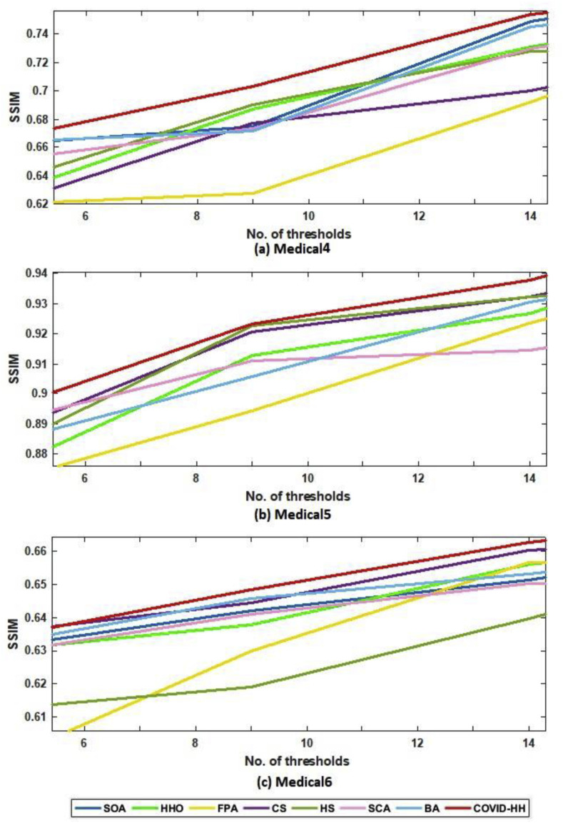
The SSIM results of Otsu's method and Kapur's entropy are presented in Table 6, Table 7 . The closer the SSIM values to 1, the better the quality of the segmented images. The tables show that the proposed algorithm has superior results in 27 from 30 cases in the case of Otsu's method; however, it has the best results in 21 from 30 cases in the case of Kapur's entropy.
Table 6.
SSIM results of Otsu's method for all algorithms.
| Image | K | Algorithms |
|||||||
|---|---|---|---|---|---|---|---|---|---|
| SOA [45] | HHOA [35] | FPA [18] | CS [19] | HS [15] | SCA [22] | BA [23] | COVID-HHOA | ||
| Medical1 | 6 | 0.5815 | 0.5817 | 0.5796 | 0.5808 | 0.5466 | 0.5733 | 0.5945 | 0.5827 |
| 8 | 0.6115 | 0.6237 | 0.6153 | 0.6222 | 0.6024 | 0.6988 | 0.7371 | 0.6256 | |
| 10 | 0.7519 | 0.8630 | 0.7505 | 0.6388 | 0.8533 | 0.7315 | 0.8871 | 0.9053 | |
| 12 | 0.7743 | 0.9055 | 0.7562 | 0.7539 | 0.9054 | 0.7549 | 0.9051 | 0.9190 | |
| 14 | 0.7841 | 0.9169 | 0.8659 | 0.9063 | 0.9120 | 0.7652 | 0.9147 | 0.9532 | |
| Medical2 | 6 | 0.5941 | 0.6004 | 0.5943 | 0.5998 | 0.5902 | 0.5892 | 0.5861 | 0.6004 |
| 8 | 0.6709 | 0.6735 | 0.6688 | 0.6647 | 0.6527 | 0.6739 | 0.6698 | 0.6816 | |
| 10 | 0.7340 | 0.7339 | 0.7203 | 0.7299 | 0.6956 | 0.7192 | 0.7336 | 0.7342 | |
| 12 | 0.7607 | 0.7722 | 0.7427 | 0.7508 | 0.7195 | 0.7513 | 0.7757 | 0.7735 | |
| 14 | 0.7848 | 0.8087 | 0.7980 | 0.7923 | 0.7708 | 0.7729 | 0.8280 | 0.8151 | |
| Medical3 | 6 | 0.8261 | 0.8259 | 0.7993 | 0.7977 | 0.8051 | 0.8299 | 0.8399 | 0.8768 |
| 8 | 0.6902 | 0.6957 | 0.6951 | 0.6961 | 0.6827 | 0.6859 | 0.6817 | 0.6961 | |
| 10 | 0.7996 | 0.8219 | 0.8125 | 0.8197 | 0.7072 | 0.7128 | 0.7797 | 0.8257 | |
| 12 | 0.8185 | 0.8550 | 0.8340 | 0.8528 | 0.8352 | 0.7662 | 0.8356 | 0.8562 | |
| 14 | 0.8497 | 0.8811 | 0.8738 | 0.8719 | 0.8374 | 0.8307 | 0.8571 | 0.8827 | |
| 6 | 0.8688 | 0.9032 | 0.8820 | 0.8910 | 0.8688 | 0.8533 | 0.8984 | 0.9038 | |
| Medical4 | 8 | 0.6929 | 0.6939 | 0.6762 | 0.6854 | 0.6508 | 0.6775 | 0.6835 | 0.6946 |
| 10 | 0.7199 | 0.8297 | 0.7206 | 0.7223 | 0.7474 | 0.7570 | 0.7935 | 0.8412 | |
| 12 | 0.8475 | 0.8793 | 0.8022 | 0.7453 | 0.7929 | 0.7857 | 0.7987 | 0.8848 | |
| 14 | 0.8498 | 0.8854 | 0.8211 | 0.7895 | 0.8438 | 0.7948 | 0.8302 | 0.9090 | |
| 6 | 0.8748 | 0.8891 | 0.8728 | 0.8721 | 0.8835 | 0.8017 | 0.9020 | 0.9236 | |
| Medical5 | 8 | 0.8840 | 0.9021 | 0.9022 | 0.9020 | 0.8587 | 0.8741 | 0.8841 | 0.9029 |
| 10 | 0.9355 | 0.9361 | 0.9367 | 0.9367 | 0.9201 | 0.9237 | 0.9279 | 0.9373 | |
| 12 | 0.9477 | 0.9541 | 0.9452 | 0.9547 | 0.9256 | 0.9327 | 0.9546 | 0.9551 | |
| 14 | 0.9484 | 0.9649 | 0.9596 | 0.9580 | 0.9468 | 0.9529 | 0.9624 | 0.9655 | |
| 6 | 0.9552 | 0.9726 | 0.9679 | 0.9692 | 0.9607 | 0.9573 | 0.9711 | 0.9739 | |
| Medical6 | 8 | 0.7027 | 0.8478 | 0.8118 | 0.8183 | 0.8683 | 0.6648 | 0.7568 | 0.8672 |
| 10 | 0.7217 | 0.8651 | 0.8401 | 0.8784 | 0.8715 | 0.6813 | 0.8186 | 0.8859 | |
| 12 | 0.7654 | 0.8799 | 0.8577 | 0.8900 | 0.8730 | 0.8025 | 0.8215 | 0.9037 | |
| 14 | 0.8159 | 0.8948 | 0.8660 | 0.8987 | 0.8996 | 0.8749 | 0.8490 | 0.9239 | |
| K | 0.8440 | 0.9013 | 0.9153 | 0.9146 | 0.9407 | 0.9246 | 0.9061 | 0.9451 | |
Table 7.
SSIM results of Kapur's entropy for all algorithms.
| Image | K | Algorithms |
|||||||
|---|---|---|---|---|---|---|---|---|---|
| SOA [45] | HHOA [35] | FPA [18] | CS [19] | HS [15] | SCA [22] | BA [23] | COVID-HHOA | ||
| Medical1 | 6 | 0.5585 | 0.5633 | 0.5626 | 0.5126 | 0.5394 | 0.5548 | 0.5601 | 0.5641 |
| 8 | 0.5823 | 0.5806 | 0.5638 | 0.5801 | 0.5785 | 0.5732 | 0.5779 | 0.5855 | |
| 10 | 0.5989 | 0.5995 | 0.5909 | 0.5816 | 0.5871 | 0.5956 | 0.5973 | 0.6048 | |
| 12 | 0.6166 | 0.6217 | 0.6054 | 0.6027 | 0.6008 | 0.6082 | 0.6253 | 0.6244 | |
| 14 | 0.6392 | 0.6342 | 0.6336 | 0.6354 | 0.6169 | 0.6332 | 0.6345 | 0.6447 | |
| Medical2 | 6 | 0.5761 | 0.5558 | 0.5814 | 0.6086 | 0.6108 | 0.5853 | 0.5688 | 0.5788 |
| 8 | 0.6565 | 0.6564 | 0.6581 | 0.6488 | 0.6691 | 0.6681 | 0.6533 | 0.6720 | |
| 10 | 0.7200 | 0.7021 | 0.6883 | 0.6527 | 0.7017 | 0.6964 | 0.7025 | 0.7270 | |
| 12 | 0.7445 | 0.7422 | 0.7418 | 0.7230 | 0.7038 | 0.7456 | 0.7599 | 0.7649 | |
| 14 | 0.7577 | 0.7848 | 0.7718 | 0.7506 | 0.7567 | 0.7740 | 0.7807 | 0.7907 | |
| Medical3 | 6 | 0.6471 | 0.6464 | 0.6453 | 0.6352 | 0.6387 | 0.6397 | 0.6513 | 0.6482 |
| 8 | 0.6888 | 0.6949 | 0.6910 | 0.6918 | 0.6952 | 0.6841 | 0.6950 | 0.6985 | |
| 10 | 0.7388 | 0.7480 | 0.7097 | 0.7437 | 0.7085 | 0.7379 | 0.7385 | 0.7477 | |
| 12 | 0.7523 | 0.7687 | 0.7408 | 0.7579 | 0.7409 | 0.7634 | 0.7748 | 0.7789 | |
| 14 | 0.7899 | 0.7924 | 0.7499 | 0.7897 | 0.7800 | 0.7671 | 0.8067 | 0.8424 | |
| Medical4 | 6 | 0.5623 | 0.5478 | 0.5994 | 0.5531 | 0.5854 | 0.5529 | 0.5346 | 0.5566 |
| 8 | 0.6601 | 0.6193 | 0.6186 | 0.6129 | 0.6284 | 0.6478 | 0.6628 | 0.6614 | |
| 10 | 0.6743 | 0.6872 | 0.6274 | 0.6773 | 0.6901 | 0.6729 | 0.6712 | 0.7033 | |
| 12 | 0.7491 | 0.7311 | 0.6919 | 0.7003 | 0.7278 | 0.7297 | 0.7454 | 0.7537 | |
| 14 | 0.7764 | 0.7603 | 0.7676 | 0.7382 | 0.7320 | 0.7659 | 0.7666 | 0.7777 | |
| Medical5 | 6 | 0.8266 | 0.8357 | 0.8094 | 0.8598 | 0.8313 | 0.8300 | 0.8326 | 0.8385 |
| 8 | 0.8763 | 0.8703 | 0.8681 | 0.8831 | 0.8771 | 0.8879 | 0.8814 | 0.8913 | |
| 10 | 0.9187 | 0.9128 | 0.8942 | 0.9206 | 0.9227 | 0.9109 | 0.9057 | 0.9233 | |
| 12 | 0.9262 | 0.9267 | 0.9235 | 0.9321 | 0.9322 | 0.9146 | 0.9305 | 0.9376 | |
| 14 | 0.9453 | 0.9543 | 0.9481 | 0.9518 | 0.9387 | 0.9296 | 0.9461 | 0.9613 | |
| Medical6 | 6 | 0.6015 | 0.6064 | 0.5905 | 0.6248 | 0.6047 | 0.6142 | 0.6019 | 0.6101 |
| 8 | 0.6299 | 0.6296 | 0.5931 | 0.6347 | 0.6115 | 0.6281 | 0.6309 | 0.6325 | |
| 10 | 0.6421 | 0.6379 | 0.6299 | 0.6445 | 0.6189 | 0.6410 | 0.6459 | 0.6485 | |
| 12 | 0.6513 | 0.6561 | 0.6566 | 0.6603 | 0.6398 | 0.6502 | 0.6531 | 0.6627 | |
| 14 | 0.6655 | 0.6663 | 0.6592 | 0.6642 | 0.6625 | 0.6542 | 0.6625 | 0.6717 | |
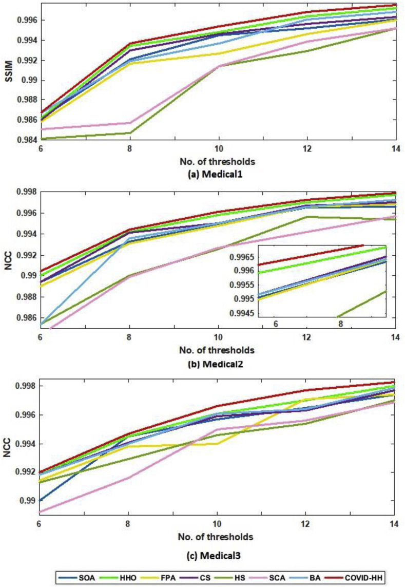
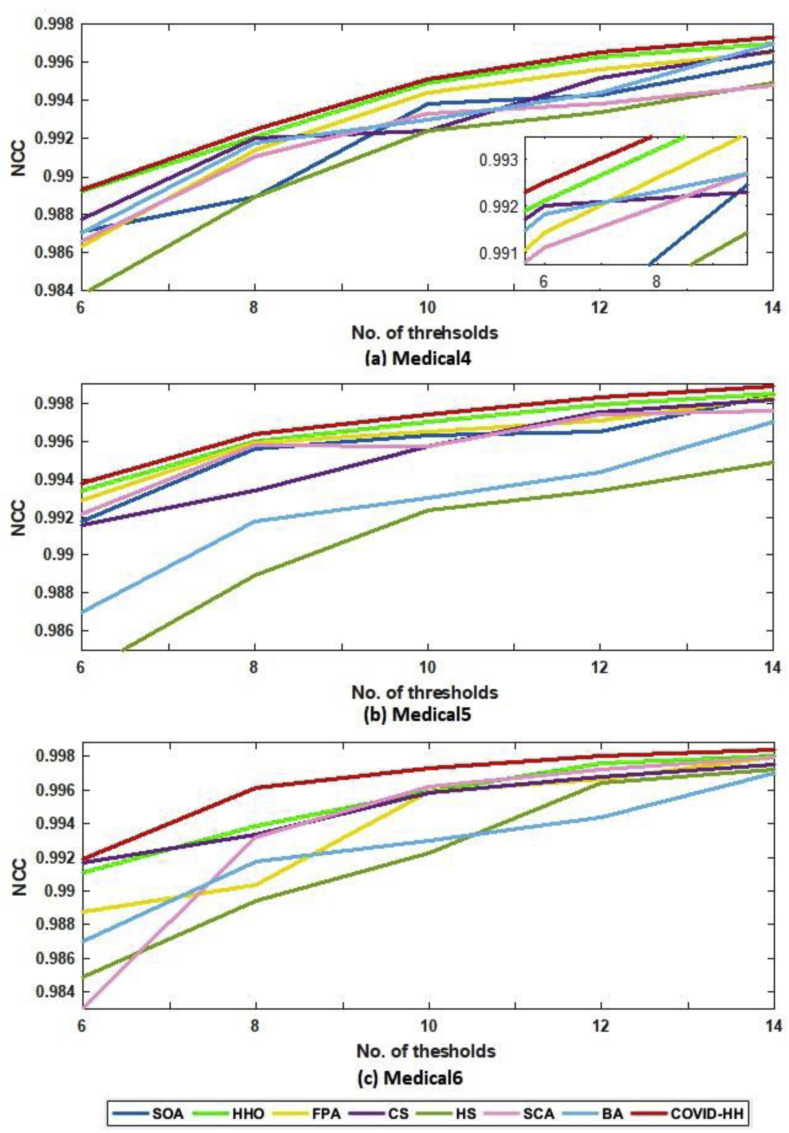
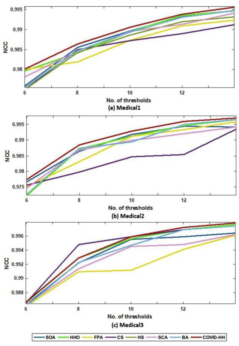
In addition to PSNR and SSIM results, the NCC results are presented to prove the high quality of the segmented images produced by the proposed algorithm. The NCC values produced by all algorithms for all 2D images using Otsu's method and Kapur's entropy are shown in Table 8, Table 9 . It can be seen that the proposed algorithm exceeds all state-of-the-art algorithms in terms of NCC values in all cases except one case in Otsu's method results and 3 cases in Kapur's entropy results.
Table 8.
NCC results of Otsu's method for all algorithms.
| Image | K | Algorithms |
|||||||
|---|---|---|---|---|---|---|---|---|---|
| SOA [45] | HHOA [35] | FPA [18] | CS [19] | HS [15] | SCA [22] | BA [23] | COVID-HHOA | ||
| Medical1 | 4 | 0.9727 | 0.9734 | 0.9722 | 0.9734 | 0.9730 | 0.9723 | 0.9855 | 0.9734 |
| 6 | 0.9862 | 0.9862 | 0.9858 | 0.9860 | 0.9866 | 0.9851 | 0.9867 | 0.9868 | |
| 8 | 0.9921 | 0.9934 | 0.9917 | 0.9930 | 0.9893 | 0.9857 | 0.9919 | 0.9937 | |
| 10 | 0.9945 | 0.9948 | 0.9927 | 0.9946 | 0.9920 | 0.9914 | 0.9937 | 0.9954 | |
| 12 | 0.9952 | 0.9964 | 0.9946 | 0.9956 | 0.9942 | 0.9939 | 0.9961 | 0.9968 | |
| 14 | 0.9961 | 0.9972 | 0.9960 | 0.9963 | 0.9949 | 0.9952 | 0.9968 | 0.9975 | |
| Medical2 | 6 | 0.9894 | 0.9900 | 0.9890 | 0.9894 | 0.9854 | 0.9844 | 0.9854 | 0.9905 |
| 8 | 0.9933 | 0.9942 | 0.9931 | 0.9941 | 0.9900 | 0.9899 | 0.9936 | 0.9944 | |
| 10 | 0.9949 | 0.9958 | 0.9948 | 0.9950 | 0.9926 | 0.9927 | 0.9950 | 0.9961 | |
| 12 | 0.9965 | 0.9970 | 0.9966 | 0.9967 | 0.9956 | 0.9942 | 0.9966 | 0.9972 | |
| 14 | 0.9966 | 0.9977 | 0.9968 | 0.9970 | 0.9954 | 0.9957 | 0.9972 | 0.9979 | |
| Medical3 | 6 | 0.9900 | 0.9918 | 0.9914 | 0.9918 | 0.9913 | 0.9892 | 0.9918 | 0.9920 |
| 8 | 0.9945 | 0.9945 | 0.9938 | 0.9941 | 0.9929 | 0.9916 | 0.9940 | 0.9947 | |
| 10 | 0.9957 | 0.9961 | 0.9940 | 0.9959 | 0.9946 | 0.9950 | 0.9961 | 0.9966 | |
| 12 | 0.9965 | 0.9970 | 0.9971 | 0.9963 | 0.9954 | 0.9956 | 0.9964 | 0.9977 | |
| 14 | 0.9974 | 0.9980 | 0.9974 | 0.9977 | 0.9970 | 0.9969 | 0.9979 | 0.9983 | |
| Medical4 | 6 | 0.9871 | 0.9893 | 0.9863 | 0.9877 | 0.9838 | 0.9866 | 0.9870 | 0.9893 |
| 8 | 0.9889 | 0.9921 | 0.9914 | 0.9920 | 0.9889 | 0.9911 | 0.9918 | 0.9925 | |
| 10 | 0.9938 | 0.9949 | 0.9944 | 0.9924 | 0.9924 | 0.9933 | 0.9930 | 0.9951 | |
| 12 | 0.9943 | 0.9963 | 0.9956 | 0.9952 | 0.9934 | 0.9938 | 0.9944 | 0.9965 | |
| 14 | 0.9960 | 0.9970 | 0.9965 | 0.9966 | 0.9949 | 0.9948 | 0.9970 | 0.9973 | |
| Medical5 | 6 | 0.9918 | 0.9934 | 0.9929 | 0.9934 | 0.9916 | 0.9912 | 0.9922 | 0.9938 |
| 8 | 0.9956 | 0.9960 | 0.9959 | 0.9957 | 0.9934 | 0.9930 | 0.9958 | 0.9964 | |
| 10 | 0.9963 | 0.9970 | 0.9965 | 0.9966 | 0.9957 | 0.9961 | 0.9957 | 0.9974 | |
| 12 | 0.9965 | 0.9979 | 0.9971 | 0.9978 | 0.9975 | 0.9967 | 0.9974 | 0.9983 | |
| 14 | 0.9984 | 0.9985 | 0.9983 | 0.9983 | 0.9982 | 0.9982 | 0.9976 | 0.9989 | |
| Medical6 | 6 | 0.9900 | 0.9911 | 0.9887 | 0.9917 | 0.9849 | 0.9909 | 0.9831 | 0.9919 |
| 8 | 0.9933 | 0.9939 | 0.9904 | 0.9934 | 0.9894 | 0.9928 | 0.9932 | 0.9961 | |
| 10 | 0.9943 | 0.9959 | 0.9959 | 0.9958 | 0.9923 | 0.9943 | 0.9962 | 0.9973 | |
| 12 | 0.9965 | 0.9976 | 0.9966 | 0.9968 | 0.9964 | 0.9962 | 0.9972 | 0.9980 | |
| 14 | 0.9977 | 0.9980 | 0.9979 | 0.9975 | 0.9972 | 0.9976 | 0.9979 | 0.9984 | |
Table 9.
NCC results of Kapur's entropy for all algorithms.
| Image | K | Algorithms |
|||||||
|---|---|---|---|---|---|---|---|---|---|
| SOA [45] | HHOA [35] | FPA [18] | CS [19] | HS [15] | SCA [22] | BA [23] | COVID-HHOA | ||
| Medical1 | 6 | 0.9759 | 0.9796 | 0.9800 | 0.9750 | 0.9750 | 0.9781 | 0.9755 | 0.9801 |
| 8 | 0.9855 | 0.9841 | 0.9818 | 0.9850 | 0.9842 | 0.9846 | 0.9847 | 0.9864 | |
| 10 | 0.9896 | 0.9894 | 0.9873 | 0.9872 | 0.9886 | 0.9895 | 0.9893 | 0.9905 | |
| 12 | 0.9931 | 0.9935 | 0.9909 | 0.9890 | 0.9919 | 0.9913 | 0.9930 | 0.9938 | |
| 14 | 0.9947 | 0.9946 | 0.9923 | 0.9912 | 0.9931 | 0.9941 | 0.9947 | 0.9956 | |
| Medical2 | 6 | 0.9767 | 0.9724 | 0.9751 | 0.9756 | 0.9765 | 0.9747 | 0.9728 | 0.9774 |
| 8 | 0.9865 | 0.9872 | 0.9832 | 0.9798 | 0.9871 | 0.9868 | 0.9874 | 0.9885 | |
| 10 | 0.9918 | 0.9912 | 0.9912 | 0.9847 | 0.9908 | 0.9899 | 0.9894 | 0.9929 | |
| 12 | 0.9944 | 0.9946 | 0.9934 | 0.9854 | 0.9913 | 0.9921 | 0.9950 | 0.9959 | |
| 14 | 0.9942 | 0.9966 | 0.9959 | 0.9935 | 0.9937 | 0.9942 | 0.9966 | 0.9970 | |
| Medical3 | 6 | 0.9863 | 0.9866 | 0.9861 | 0.9866 | 0.9843 | 0.9863 | 0.9861 | 0.9867 |
| 8 | 0.9922 | 0.9929 | 0.9909 | 0.9948 | 0.9920 | 0.9914 | 0.9923 | 0.9929 | |
| 10 | 0.9955 | 0.9956 | 0.9912 | 0.9959 | 0.9925 | 0.9945 | 0.9947 | 0.9959 | |
| 12 | 0.9959 | 0.9969 | 0.9941 | 0.9969 | 0.9935 | 0.9948 | 0.9969 | 0.9972 | |
| 14 | 0.9964 | 0.9976 | 0.9961 | 0.9974 | 0.9953 | 0.9962 | 0.9974 | 0.9978 | |
| Medical4 | 6 | 0.9709 | 0.9691 | 0.9779 | 0.9693 | 0.9755 | 0.9679 | 0.9663 | 0.9719 |
| 8 | 0.9843 | 0.9821 | 0.9789 | 0.9728 | 0.9824 | 0.9822 | 0.9842 | 0.9855 | |
| 10 | 0.9877 | 0.9877 | 0.9805 | 0.9845 | 0.9864 | 0.9870 | 0.9856 | 0.9895 | |
| 12 | 0.9932 | 0.9924 | 0.9858 | 0.9892 | 0.9909 | 0.9913 | 0.9934 | 0.9939 | |
| 14 | 0.9942 | 0.9942 | 0.9926 | 0.9924 | 0.9916 | 0.9926 | 0.9942 | 0.9950 | |
| Medical5 | 6 | 0.9870 | 0.9857 | 0.9840 | 0.9916 | 0.9844 | 0.9843 | 0.9839 | 0.9866 |
| 8 | 0.9934 | 0.9920 | 0.9907 | 0.9950 | 0.9931 | 0.9925 | 0.9942 | 0.9946 | |
| 10 | 0.9954 | 0.9954 | 0.9929 | 0.9960 | 0.9953 | 0.9953 | 0.9953 | 0.9964 | |
| 12 | 0.9962 | 0.9962 | 0.9962 | 0.9969 | 0.9963 | 0.9962 | 0.9970 | 0.9975 | |
| 14 | 0.9978 | 0.9980 | 0.9962 | 0.9980 | 0.9972 | 0.9972 | 0.9976 | 0.9983 | |
| Medical6 | 6 | 0.9871 | 0.9882 | 0.9765 | 0.9913 | 0.9828 | 0.9879 | 0.9850 | 0.9884 |
| 8 | 0.9916 | 0.9920 | 0.9789 | 0.9920 | 0.9852 | 0.9898 | 0.9911 | 0.9923 | |
| 10 | 0.9932 | 0.9929 | 0.9893 | 0.9933 | 0.9861 | 0.9911 | 0.9932 | 0.9942 | |
| 12 | 0.9937 | 0.9946 | 0.9935 | 0.9946 | 0.9922 | 0.9934 | 0.9941 | 0.9950 | |
| 14 | 0.9945 | 0.9952 | 0.9945 | 0.9950 | 0.9936 | 0.9944 | 0.9947 | 0.9955 | |
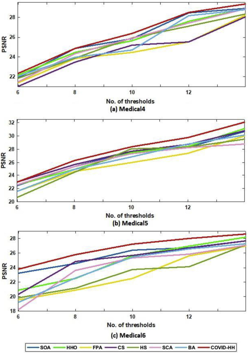
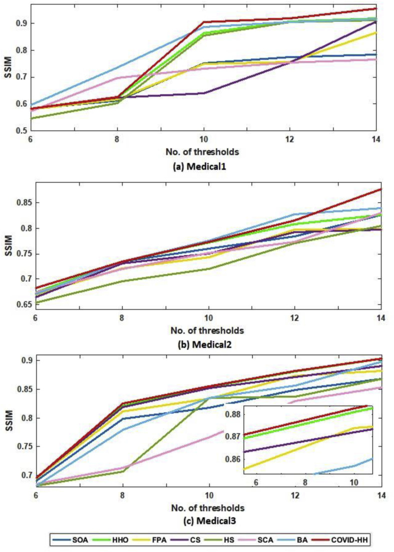
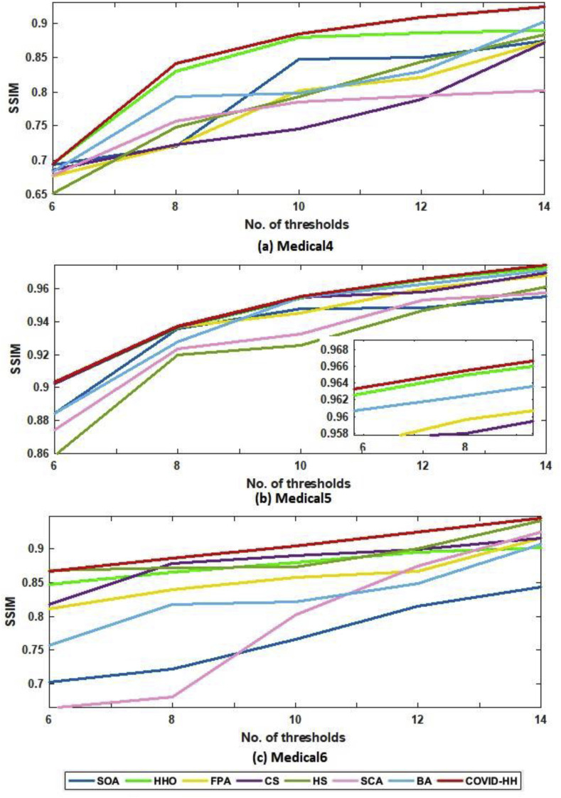
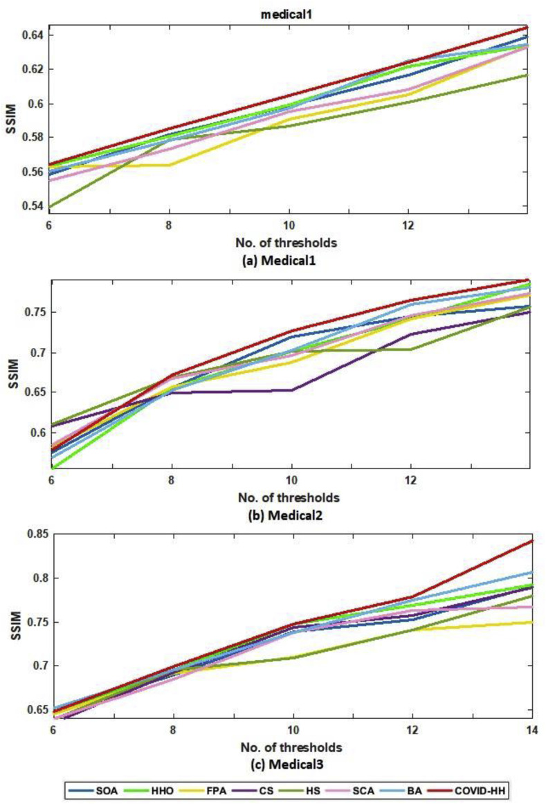
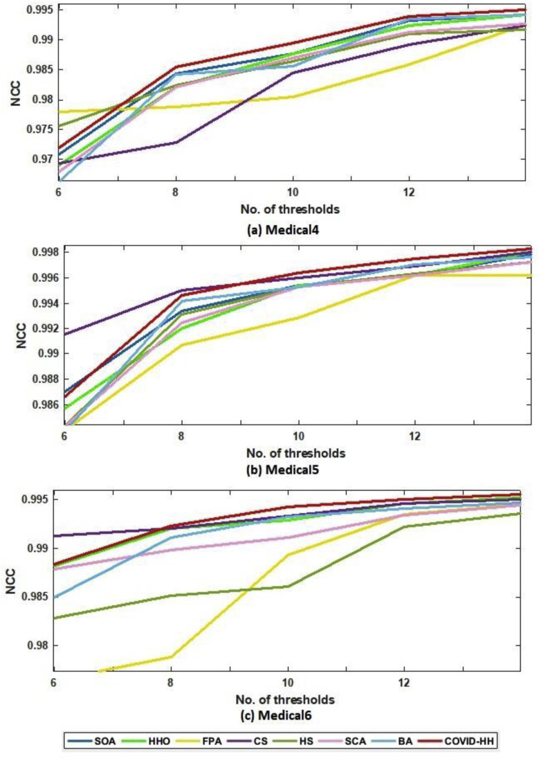
The relationship between the number of thresholds and PSNR, SSIM, and NCC for Otsu's method and Kapur's entropy is shown in Fig. 10 to Fig. 11, Fig. 12, Fig. 13, Fig. 14, Fig. 15 , respectively. Each one is split into two figures (a and b) for more clarity.
Fig. 10.
(a): PSNR results of Otsu's method for all algorithms at each threshold level for Medical1, Medical2, and Medical3 images.
(b): PSNR results of Otsu's method for all algorithms at each threshold level for Medical4, Medical5, and Medical6 images.
Fig. 11.
(a): PSNR results of Kapur's entropy for all algorithms at each threshold level for Medical1. Medical2 and Medical3 images.
(b): PSNR results of Kapur's entropy for all algorithms at each threshold level for Medical4, Medical5, and Medical6 images.
Fig. 12.
(a): SSIM results of Otsu's method for all algorithms at each threshold level for Medical1, Medical2, and Medical3 images.
(b): SSIM results of Otsu's method for all algorithms at each threshold level for Medical4, Medical5, and Medical6 images.
Fig. 13.
(a): SSIM results of Kapur's entropy for all algorithms at each threshold level for Medical1, Medical2, and Medical3 images.
(b): SSIM results of Kapur's entropy for all algorithms at each threshold level for Medical4, Medical5, and Medical6 images.
Fig. 14.
(a): NCC results from Otsu's method for all algorithms at each threshold level for Medical1, Medical2, and Medical3 images.
Fig. 14 (b): NCC results from Otsu's method for all algorithms at each threshold level for Medical4, Medical5, and Medical6 images.
Fig. 15.
(a): NCC results in Kapur's entropy for all algorithms at each threshold level for Medical1, Medical2, and Medical3 images.
(b): NCC results in Kapur's entropy for all algorithms at each threshold level for Medical4, Medical5, and Medical6 images.
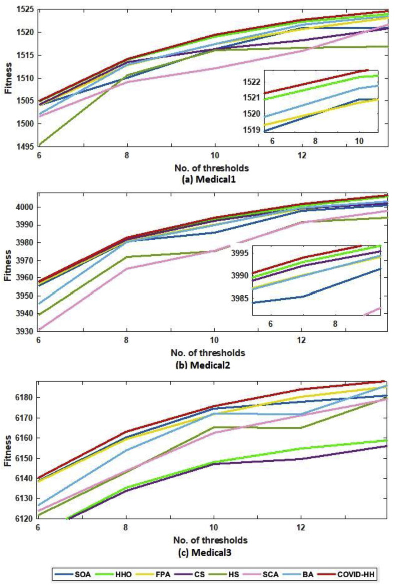
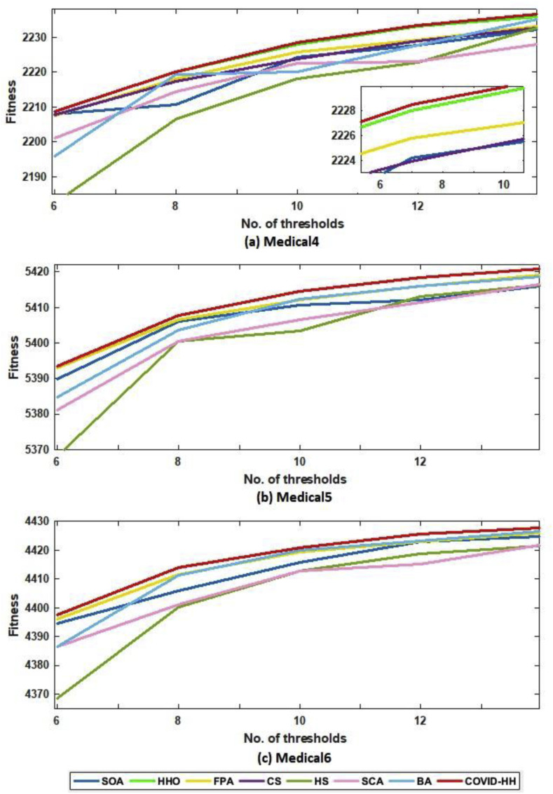
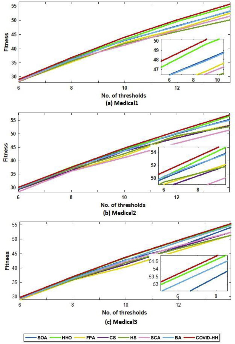
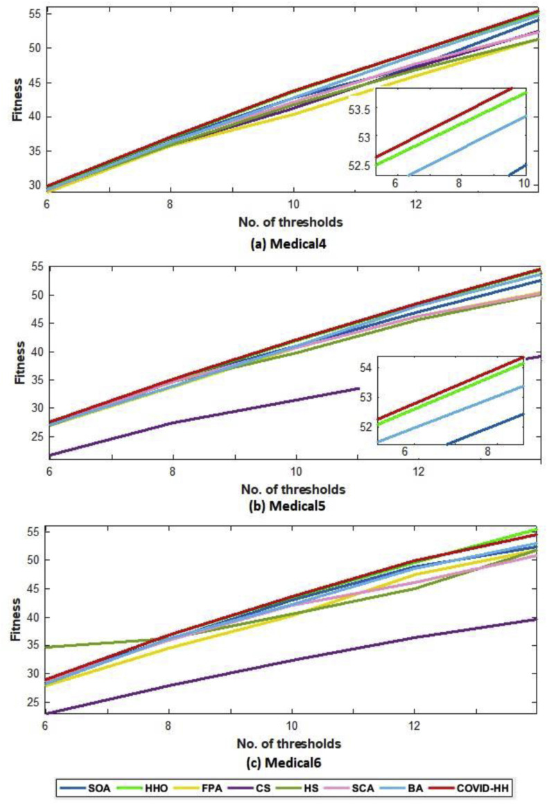
According to the fitness function, we compared the proposed algorithm to the other algorithms in terms of the best fitness value obtained from running each algorithm 30 times with Otsu's method and Kapur's entropy. Higher fitness function values indicate higher quality of the solutions produced by the algorithm. The best fitness values for all algorithms using Otsu's method and Kapur's entropy are shown in Table 10, Table 11 . The relationship between the thresholds and the fitness values is shown in Fig. 16 (a, b) and 17 (a, b) for Otsu's method and Kapur's entropy, respectively. Although all algorithms have relative fitness values, the proposed algorithm slightly exceeds them in almost all cases, indicating its ability to find high-quality solutions.
Table 10.
Best fitness values of Ostu's method for all algorithms.
| Image | K | Algorithms |
|||||||
|---|---|---|---|---|---|---|---|---|---|
| SOA [45] | HHOA [35] | FPA [18] | CS [19] | HS [15] | SCA [22] | BA [23] | COVID-HHOA | ||
| Medical1 | 6 | 1.5041e+03 | 1.5049e+03 | 1.5041e+03 | 1.5042e+03 | 1.4955e+03 | 1.5016e+03 | 1.5022e+03 | 1.5050e+03 |
| 8 | 1.5101e+03 | 1.5140e+03 | 1.5128e+03 | 1.5135e+03 | 1.5107e+03 | 1.5092e+03 | 1.5130e+03 | 1.5142e+03 | |
| 10 | 1.5164e+03 | 1.5191e+03 | 1.5175e+03 | 1.5163e+03 | 1.5161e+03 | 1.5122e+03 | 1.5175e+03 | 1.5195e+03 | |
| 12 | 1.5209e+03 | 1.5223e+03 | 1.5207e+03 | 1.5183e+03 | 1.5166e+03 | 1.5159e+03 | 1.5216e+03 | 1.5227e+03 | |
| 14 | 1.5210e+03 | 1.5239e+03 | 1.5232e+03 | 1.5209e+03 | 1.5169e+03 | 1.5218e+03 | 1.5235e+03 | 1.5246e+03 | |
| Medical2 | 6 | 3.9554e+03 | 3.9577e+03 | 3.9566e+03 | 3.9577e+03 | 3.9395e+03 | 3.9312e+03 | 3.9459e+03 | 3.9580e+03 |
| 8 | 3.9808e+03 | 3.9821e+03 | 3.9811e+03 | 3.9817e+03 | 3.9721e+03 | 3.9654e+03 | 3.9805e+03 | 3.9829e+03 | |
| 10 | 3.9855e+03 | 3.9930e+03 | 3.9901e+03 | 3.9922e+03 | 3.9752e+03 | 3.9754e+03 | 3.9900e+03 | 3.9940e+03 | |
| 12 | 3.9980e+03 | 4.0008e+03 | 3.9988e+03 | 3.9992e+03 | 3.9916e+03 | 3.9913e+03 | 3.9995e+03 | 4.0016e+03 | |
| 14 | 4.0010e+03 | 4.0061e+03 | 4.0028e+03 | 4.0020e+03 | 3.9941e+03 | 3.9980e+03 | 4.0032e+03 | 4.0067e+03 | |
| Medical3 | 6 | 6.1387e+03 | 6.1128e+03 | 6.1383e+03 | 6.1128e+03 | 6.1219e+03 | 6.1240e+03 | 6.1267e+03 | 6.1402e+03 |
| 8 | 6.1603e+03 | 6.1352e+03 | 6.1594e+03 | 6.1337e+03 | 6.1430e+03 | 6.1436e+03 | 6.1539e+03 | 6.1633e+03 | |
| 10 | 6.1744e+03 | 6.1482e+03 | 6.1717e+03 | 6.1470e+03 | 6.1652e+03 | 6.1627e+03 | 6.1721e+03 | 6.1757e+03 | |
| 12 | 6.1780e+03 | 6.1549e+03 | 6.1804e+03 | 6.1497e+03 | 6.1650e+03 | 6.1711e+03 | 6.1719e+03 | 6.1841e+03 | |
| 14 | 6.1809e+03 | 6.1590e+03 | 6.1854e+03 | 6.1564e+03 | 6.1801e+03 | 6.1792e+03 | 6.1863e+03 | 6.1882e+03 | |
| Medical4 | 6 | 2.2081e+03 | 2.2089e+03 | 2.2077e+03 | 2.2079e+03 | 2.1824e+03 | 2.2009e+03 | 2.1957e+03 | 2.2088e+03 |
| 8 | 2.2108e+03 | 2.2201e+03 | 2.2181e+03 | 2.2174e+03 | 2.2065e+03 | 2.2144e+03 | 2.2193e+03 | 2.2200e+03 | |
| 10 | 2.2242e+03 | 2.2280e+03 | 2.2258e+03 | 2.2239e+03 | 2.2181e+03 | 2.2226e+03 | 2.2202e+03 | 2.2285e+03 | |
| 12 | 2.2277e+03 | 2.2331e+03 | 2.2292e+03 | 2.2289e+03 | 2.2227e+03 | 2.2231e+03 | 2.2276e+03 | 2.2333e+03 | |
| 14 | 2.2322e+03 | 2.2358e+03 | 2.2332e+03 | 2.2328e+03 | 2.2328e+03 | 2.2280e+03 | 2.2353e+03 | 2.2367e+03 | |
| Medical5 | 6 | 5.3898e+03 | 4.8687e+03 | 5.3931e+03 | 4.8687e+03 | 5.3681e+03 | 5.3812e+03 | 5.3847e+03 | 5.3936e+03 |
| 8 | 5.4061e+03 | 4.8825e+03 | 5.4065e+03 | 4.8824e+03 | 5.4006e+03 | 5.4007e+03 | 5.4038e+03 | 5.4077e+03 | |
| 10 | 5.4108e+03 | 4.8893e+03 | 5.4122e+03 | 4.8893e+03 | 5.4034e+03 | 5.4066e+03 | 5.4125e+03 | 5.4145e+03 | |
| 12 | 5.4122e+03 | 4.8929e+03 | 5.4161e+03 | 4.8915e+03 | 5.4131e+03 | 5.4115e+03 | 5.4160e+03 | 5.4184e+03 | |
| 14 | 5.4160e+03 | 4.8955e+03 | 5.4192e+03 | 4.8941e+03 | 5.4164e+03 | 5.4167e+03 | 5.4186e+03 | 5.4208e+03 | |
| Medical6 | 6 | 4.3948e+03 | 4.2056e+03 | 4.3961e+03 | 4.2055e+03 | 4.3687e+03 | 4.3865e+03 | 4.3865e+03 | 4.3978e+03 |
| 8 | 4.4059e+03 | 4.2211e+03 | 4.4117e+03 | 4.2207e+03 | 4.4002e+03 | 4.4012e+03 | 4.4113e+03 | 4.4139e+03 | |
| 10 | 4.4157e+03 | 4.2287e+03 | 4.4193e+03 | 4.2282e+03 | 4.4129e+03 | 4.4129e+03 | 4.4199e+03 | 4.4209e+03 | |
| 12 | 4.4230e+03 | 4.2326e+03 | 4.4230e+03 | 4.2318e+03 | 4.4188e+03 | 4.4153e+03 | 4.4231e+03 | 4.4257e+03 | |
| 14 | 4.4246e+03 | 4.2343e+03 | 4.4259e+03 | 4.2340e+03 | 4.4215e+03 | 4.4219e+03 | 4.4265e+03 | 4.4278e+03 | |
Table 11.
Best fitness values of Kapur's entropy for all algorithms.
| Image | K | Algorithms |
|||||||
|---|---|---|---|---|---|---|---|---|---|
| SOA [45] | HHOA [35] | FPA [18] | CS [19] | HS [15] | SCA [22] | BA [23] | COVID-HHOA | ||
| Medical1 | 6 | 29.1150 | 29.1440 | 28.4842 | 28.5451 | 28.4039 | 28.4511 | 28.9466 | 29.1497 |
| 8 | 36.4624 | 36.6540 | 35.1770 | 35.7679 | 35.6282 | 36.1923 | 36.0033 | 36.7475 | |
| 10 | 42.8551 | 43.2945 | 42.1935 | 42.2456 | 41.7597 | 41.3143 | 42.9482 | 44.0402 | |
| 12 | 48.0268 | 49.6176 | 46.7989 | 46.3681 | 45.9796 | 46.5262 | 47.9183 | 50.1440 | |
| 14 | 53.1311 | 54.8167 | 52.5195 | 52.4872 | 50.0722 | 51.4593 | 53.2681 | 55.7106 | |
| Medical2 | 6 | 30.0560 | 30.0624 | 29.2634 | 29.3301 | 29.1013 | 29.5610 | 29.7242 | 30.1228 |
| 8 | 37.4817 | 37.6122 | 36.3408 | 36.4637 | 36.4182 | 37.0426 | 37.3252 | 37.5760 | |
| 10 | 44.1656 | 44.5172 | 41.9516 | 43.6734 | 42.7747 | 42.7167 | 43.6806 | 44.7035 | |
| 12 | 50.0224 | 50.2347 | 49.0840 | 48.5610 | 47.7153 | 49.4137 | 50.2842 | 50.9972 | |
| 14 | 55.3181 | 56.5864 | 53.2115 | 53.1273 | 52.3780 | 52.7230 | 55.0156 | 56.9942 | |
| Medical3 | 6 | 29.4506 | 29.4480 | 28.6691 | 23.1739 | 28.4564 | 29.4011 | 29.2656 | 29.4703 |
| 8 | 37.2324 | 37.3536 | 35.0245 | 28.3095 | 35.1488 | 36.4795 | 36.0121 | 37.3482 | |
| 10 | 43.5538 | 44.2176 | 42.3845 | 32.7091 | 41.7464 | 42.8749 | 42.8232 | 44.3337 | |
| 12 | 49.1426 | 50.3112 | 47.7115 | 36.5965 | 47.5394 | 48.0504 | 49.5033 | 50.4694 | |
| 14 | 52.4016 | 56.0881 | 52.5454 | 40.3468 | 52.2408 | 52.9522 | 54.6020 | 56.1094 | |
| Medical4 | 6 | 29.7038 | 29.8214 | 29.0196 | 29.4504 | 29.3854 | 29.2795 | 29.4105 | 29.8370 |
| 8 | 36.5791 | 36.8520 | 35.7648 | 35.8712 | 35.9158 | 36.3379 | 36.2300 | 36.9593 | |
| 10 | 42.8729 | 43.6696 | 40.4616 | 41.3581 | 41.8134 | 42.2490 | 42.7692 | 43.7918 | |
| 12 | 47.4509 | 49.5428 | 46.0389 | 47.2014 | 46.8216 | 47.7198 | 48.9814 | 49.5914 | |
| 14 | 54.1334 | 55.1970 | 51.3232 | 52.4321 | 51.3109 | 52.4020 | 54.7969 | 55.4478 | |
| Medical5 | 6 | 27.5392 | 27.6409 | 26.9876 | 21.7552 | 26.9903 | 27.1946 | 27.1707 | 27.6422 |
| 8 | 35.0168 | 35.1453 | 33.7456 | 27.3895 | 34.5749 | 34.5868 | 33.8298 | 35.2417 | |
| 10 | 41.1285 | 42.0444 | 40.8043 | 31.4742 | 39.7802 | 40.7294 | 41.1127 | 42.1571 | |
| 12 | 47.0732 | 48.4408 | 46.2316 | 35.6166 | 45.5961 | 46.2532 | 48.1818 | 48.5939 | |
| 14 | 52.6506 | 54.3979 | 50.5047 | 39.2780 | 50.1560 | 50.3272 | 53.5915 | 54.5965 | |
| Medical6 | 6 | 28.9177 | 29.0004 | 27.9225 | 22.9562 | 34.5683 | 28.6647 | 28.2243 | 29.0004 |
| 8 | 36.0479 | 36.9304 | 34.5297 | 27.9091 | 36.3630 | 35.8314 | 36.3014 | 36.9257 | |
| 10 | 43.0778 | 43.5536 | 40.2129 | 32.3120 | 40.6346 | 42.0560 | 42.1871 | 43.6132 | |
| 12 | 48.8374 | 49.6670 | 47.4302 | 36.4025 | 45.0181 | 46.1182 | 48.5252 | 49.8300 | |
| 14 | 52.3678 | 55.3890 | 51.7384 | 39.7488 | 51.7612 | 50.7992 | 52.9835 | 54.4504 | |
Fig. 16.
(a): The best fitness values of Otsu's method for all algorithms for Medical1, Medical2, and Medical3 images.
(b): The best fitness values of Otsu's method for all algorithms for Medical4, Medical5, and Medical6 images.
Fig. 17.
(a): The best fitness values of Kapur's method for all algorithms for Medical1, Medical2, and Medical3 images.
(b): The best fitness values of Kapur's method for all algorithms for Medical4, Medical5, and Medical6 images.
6.4.2. Experimental results for 3D medical images
In this section, the performance of the proposed algorithm in 3D medical image segmentation is assessed according to the same evaluation metrics mentioned above. The proposed algorithm and seven well-known metaheuristic techniques are applied to 6 different volumetric medical images to determine the optimal threshold values to segment the slices of these images. We utilized the same parameter settings and threshold levels as in the case of 2D medical images.
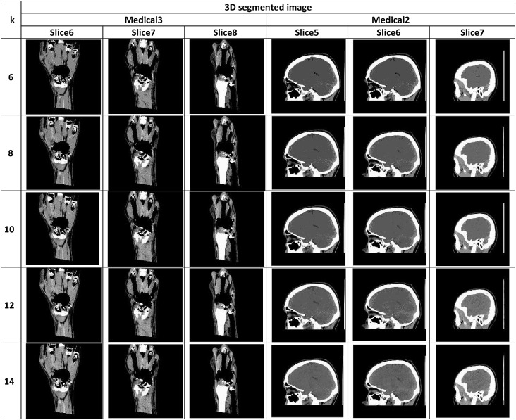
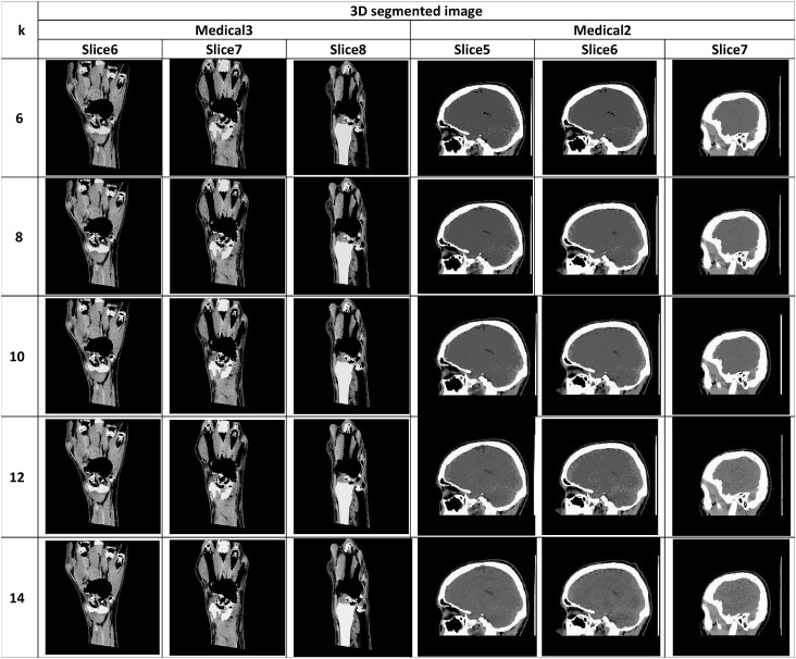
The segmented image slices from applying the proposed algorithm for Otsu's method and Kapur's entropy at different threshold levels are shown in Table 14, Table 15 , respectively. The high quality of the segmented image slices is evident from their visual appearance.
Table 14.
Slices of 3D medical images segmented by the proposed COVID-HHOA algorithm using Otsu's method.
Table 15.
Slices of 3D medical images segmented by the proposed COVID-HHOA algorithm using Kapur's entropy.
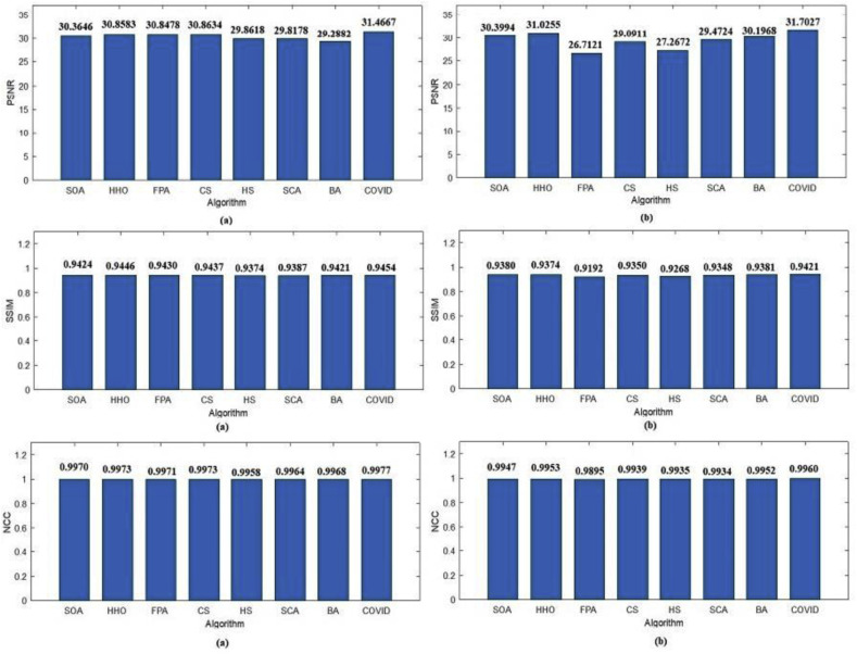
The results of PSNR, SSIM, and NCC of the proposed algorithm against its peers for Otsu's method and Kapur's entropy are given in Table 16 to Table 17, Table 18, Table 19, Table 20, Table 21 . The values in these tables, highlighted in bold, indicate the best results.
Table 16.
PSNR results of 3D medical image segmentation using Otsu's method for all algorithms.
| Image | K | Algorithms |
|||||||
|---|---|---|---|---|---|---|---|---|---|
| SOA [41] | HHOA [35] | FPA [18] | CS [19] | HS [15] | SCA [22] | BA [23] | COVID-HHOA | ||
| 3D_imag1 | 6 | 30.1961 | 30.4401 | 30.6070 | 29.5351 | 29.8018 | 30.1225 | 29.8267 | 30.6455 |
| 8 | 32.0807 | 32.4235 | 32.5736 | 31.5420 | 31.0633 | 31.4139 | 31.3611 | 32.7306 | |
| 10 | 33.7221 | 34.2130 | 34.1211 | 33.3435 | 32.6111 | 32.6553 | 32.3934 | 34.5134 | |
| 12 | 34.3873 | 35.2726 | 35.1746 | 34.6316 | 34.4152 | 34.4275 | 34.2041 | 35.6317 | |
| 14 | 35.6631 | 36.3439 | 36.3487 | 36.4534 | 35.2466 | 34.2358 | 34.5301 | 37.3705 | |
| 3D_imag2 | 6 | 28.4792 | 28.2612 | 28.5816 | 28.1514 | 28.2390 | 28.1231 | 27.4920 | 28.5700 |
| 8 | 29.9857 | 30.3715 | 30.4281 | 30.2278 | 29.2314 | 29.5801 | 29.6223 | 30.8414 | |
| 10 | 31.8611 | 32.0457 | 32.0356 | 32.1523 | 30.8432 | 30.8721 | 30.1978 | 32.5086 | |
| 12 | 32.9469 | 33.3460 | 33.1822 | 33.1939 | 31.9144 | 31.2241 | 31.4527 | 33.7971 | |
| 14 | 33.2306 | 34.3034 | 34.3424 | 34.4636 | 33.2121 | 32.7286 | 32.0812 | 34.9959 | |
| 3D_imag3 | 6 | 23.8765 | 24.5766 | 24.7164 | 24.7615 | 23.6154 | 23.5595 | 22.5702 | 25.3023 |
| 8 | 26.1167 | 26.7796 | 27.0332 | 27.1784 | 26.7589 | 27.2304 | 24.7527 | 27.6537 | |
| 10 | 27.9192 | 28.8867 | 28.3241 | 29.1432 | 27.2341 | 27.9804 | 26.4567 | 29.6654 | |
| 12 | 28.9860 | 30.3745 | 30.0778 | 31.0939 | 28.5432 | 28.4431 | 27.4352 | 31.4758 | |
| 14 | 29.2986 | 31.6990 | 31.2865 | 32.0764 | 29.4811 | 29.8310 | 28.4833 | 32.7302 | |
| 3D_imag4 | 6 | 26.9810 | 26.9321 | 27.1231 | 26.6620 | 26.8743 | 26.3212 | 25.7158 | 27.3305 |
| 8 | 29.2953 | 28.8902 | 29.5442 | 28.2524 | 28.2630 | 28.1423 | 27.5351 | 29.5858 | |
| 10 | 31.0143 | 30.5272 | 31.0023 | 31.0154 | 30.1232 | 29.5087 | 29.2950 | 31.4076 | |
| 12 | 32.1998 | 32.0870 | 32.4472 | 32.1555 | 31.1611 | 30.9122 | 30.1142 | 32.8436 | |
| 14 | 32.5924 | 33.2061 | 33.3724 | 33.2594 | 31.2641 | 32.3986 | 31.1415 | 33.8989 | |
| 3D_imag5 | 6 | 27.4326 | 28.4923 | 28.3731 | 28.1460 | 27.4155 | 28.2378 | 27.7748 | 28.4717 |
| 8 | 29.7636 | 30.2675 | 29.4632 | 30.1205 | 28.2261 | 29.4793 | 28.4571 | 30.5245 | |
| 10 | 31.3146 | 31.8957 | 31.8638 | 32.1162 | 30.7573 | 30.4451 | 30.4593 | 32.7594 | |
| 12 | 32.2885 | 33.4235 | 32.5232 | 32.7948 | 31.9792 | 31.9715 | 31.6864 | 33.7197 | |
| 14 | 32.7714 | 34.2666 | 33.6360 | 34.1648 | 33.7886 | 31.9899 | 32.0876 | 34.8721 | |
| 3D_image6 | 6 | 26.3354 | 26.4546 | 26.2072 | 26.4751 | 26.0888 | 26.1373 | 25.4470 | 26.7845 |
| 8 | 28.5190 | 28.1292 | 28.0865 | 28.3212 | 27.9585 | 27.1920 | 27.7022 | 28.4532 | |
| 10 | 29.4571 | 30.2222 | 29.8765 | 30.2512 | 29.3425 | 28.9353 | 28.234 | 30.5218 | |
| 12 | 30.4919 | 31.4218 | 31.0183 | 31.7098 | 30.2065 | 30.2410 | 29.9403 | 31.7267 | |
| 14 | 31.7326 | 32.2109 | 32.0645 | 32.5123 | 31.2352 | 31.1132 | 30.9337 | 32.6480 | |
| Average | 30.3646 | 30.8583 | 30.8478 | 30.8634 | 29.8618 | 29.8178 | 29.2882 | 31.4667 | |
Table 17.
PSNR results of 3D medical image segmentation using Kapur's method for all algorithms.
| Image | K | Algorithms |
|||||||
|---|---|---|---|---|---|---|---|---|---|
| SOA [41] | HHOA [35] | FPA [18] | CS [19] | HS [15] | SCA [22] | BA [23] | COVID-HHOA | ||
| Medical1 | 6 | 28.9391 | 28.7182 | 26.7359 | 27.8832 | 27.8761 | 28.5393 | 28.2466 | 29.0592 |
| 8 | 30.789 | 31.7338 | 27.3459 | 30.2013 | 28.3848 | 29.2610 | 31.9910 | 32.5919 | |
| 10 | 33.4462 | 34.5674 | 28.8927 | 32.7649 | 30.2011 | 31.6723 | 33.9310 | 34.3256 | |
| 12 | 34.8542 | 35.6831 | 30.5443 | 33.9639 | 31.5210 | 32.4643 | 35.436 | 36.2500 | |
| 14 | 36.1017 | 37.0353 | 32.4340 | 36.6387 | 33.1574 | 33.7446 | 36.6467 | 37.4015 | |
| Medical2 | 6 | 27.8760 | 28.1027 | 24.0359 | 25.3058 | 26.2936 | 26.8300 | 27.1412 | 28.8769 |
| 8 | 29.6887 | 30.2295 | 25.5423 | 28.4327 | 27.5561 | 28.4240 | 29.0898 | 30.9285 | |
| 10 | 30.1092 | 31.8796 | 27.3453 | 31.9067 | 29.3428 | 30.9737 | 31.9503 | 32.6432 | |
| 12 | 33.2782 | 34.2882 | 28.5334 | 33.3440 | 30.1108 | 31.6471 | 32.6461 | 34.9733 | |
| 14 | 33.7369 | 35.6173 | 29.2686 | 34.7503 | 30.1138 | 31.9441 | 33.5732 | 35.9389 | |
| Medical3 | 6 | 25.3868 | 23.6456 | 19.1499 | 22.6928 | 20.8765 | 25.0683 | 23.5777 | 25.8508 |
| 8 | 27.6444 | 25.2165 | 21.3553 | 25.7434 | 22.1535 | 26.3433 | 25.8927 | 27.3553 | |
| 10 | 28.8815 | 26.7871 | 24.6891 | 27.9029 | 25.1566 | 27.8761 | 28.0051 | 28.3343 | |
| 12 | 30.3123 | 30.4122 | 25.2345 | 30.6865 | 26.4503 | 28.4920 | 29.3453 | 32.4365 | |
| 14 | 31.2641 | 31.3217 | 26.4080 | 32.5818 | 28.6095 | 30.4881 | 30.5706 | 33.6475 | |
| Medical4 | 6 | 27.1636 | 29.3512 | 23.3768 | 22.7454 | 20.3453 | 28.3452 | 27.3451 | 29.4851 |
| 8 | 29.6801 | 30.1578 | 24.2954 | 25.1042 | 22.9910 | 29.4786 | 29.1662 | 30.3341 | |
| 10 | 31.1514 | 32.6423 | 25.9872 | 27.0787 | 25.2696 | 30.9397 | 30.4599 | 32.6304 | |
| 12 | 31.9376 | 34.1111 | 27.6909 | 30.4325 | 27.3560 | 31.6453 | 31.3344 | 34.2147 | |
| 14 | 32.8808 | 35.2234 | 30.5359 | 33.1648 | 28.0357 | 32.5760 | 32.6905 | 35.4816 | |
| Medical5 | 6 | 27.0996 | 29.8734 | 26.0212 | 23.6755 | 25.0232 | 26.4998 | 26.8532 | 30.1234 |
| 8 | 29.5678 | 31.1420 | 27.7549 | 24.6086 | 26.7692 | 28.2310 | 29.0765 | 31.6352 | |
| 10 | 31.2849 | 32.1204 | 29.4533 | 28.9561 | 29.6891 | 29.3244 | 30.4819 | 32.5461 | |
| 12 | 32.4544 | 32.6433 | 30.0826 | 30.5643 | 30.7765 | 30.6543 | 32.5921 | 33.7241 | |
| 14 | 33.8361 | 34.3116 | 31.8976 | 31.3037 | 31.4373 | 31.5773 | 33.4335 | 34.9109 | |
| Medical6 | 6 | 25.6432 | 25.2261 | 22.3990 | 24.5574 | 23.4597 | 24.6637 | 25.0497 | 25.6262 |
| 8 | 27.1155 | 28.1435 | 23.5334 | 26.7452 | 24.7891 | 27.5356 | 27.3455 | 28.5462 | |
| 10 | 29.1776 | 30.1078 | 25.5249 | 29.4057 | 26.9886 | 29.0901 | 29.6829 | 30.4483 | |
| 12 | 30.1092 | 31.5349 | 26.3562 | 30.6543 | 28.3455 | 29.6740 | 30.5332 | 31.8232 | |
| 14 | 30.5725 | 32.2195 | 27.5853 | 31.9613 | 29.8339 | 30.1687 | 31.8188 | 32.4613 | |
| Average | 30.3994 | 31.0255 | 26.7121 | 29.0911 | 27.2672 | 29.4724 | 30.1968 | 31.7027 | |
Table 18.
SSIM results of 3D medical image segmentation using Otsu's method for all algorithms.
| Image | K | Algorithms |
|||||||
|---|---|---|---|---|---|---|---|---|---|
| SOA [41] | HHOA [35] | FPA [18] | CS [19] | HS [15] | SCA [22] | BA [23] | COVID-HHOA | ||
| Medical1 | 6 | 0.9727 | 0.9740 | 0.9737 | 0.9734 | 0.9686 | 0.9719 | 0.9731 | 0.9741 |
| 8 | 0.9776 | 0.9783 | 0.9778 | 0.9781 | 0.9750 | 0.9759 | 0.9776 | 0.9785 | |
| 10 | 0.9795 | 0.9797 | 0.9797 | 0.9800 | 0.9770 | 0.9777 | 0.9790 | 0.9801 | |
| 12 | 0.9805 | 0.9811 | 0.9806 | 0.9811 | 0.9790 | 0.9794 | 0.9806 | 0.9812 | |
| 14 | 0.9811 | 0.9815 | 0.9814 | 0.9816 | 0.9800 | 0.9798 | 0.9810 | 0.9822 | |
| Medical2 | 6 | 0.9600 | 0.9599 | 0.9600 | 0.9597 | 0.9546 | 0.9555 | 0.9588 | 0.9602 |
| 8 | 0.9673 | 0.9673 | 0.9664 | 0.9674 | 0.9643 | 0.9627 | 0.9663 | 0.9676 | |
| 10 | 0.9707 | 0.9711 | 0.9698 | 0.9701 | 0.9674 | 0.9646 | 0.9703 | 0.9719 | |
| 12 | 0.9721 | 0.9733 | 0.9719 | 0.9727 | 0.9693 | 0.9697 | 0.9720 | 0.9736 | |
| 14 | 0.9721 | 0.9736 | 0.9734 | 0.9738 | 0.9714 | 0.9711 | 0.9732 | 0.9745 | |
| Medical3 | 6 | 0.9153 | 0.9171 | 0.9173 | 0.9179 | 0.9022 | 0.9042 | 0.8993 | 0.9200 |
| 8 | 0.9279 | 0.9325 | 0.9323 | 0.9287 | 0.9220 | 0.9265 | 0.9260 | 0.9347 | |
| 10 | 0.9373 | 0.9416 | 0.9387 | 0.9354 | 0.9289 | 0.9301 | 0.9378 | 0.9419 | |
| 12 | 0.9404 | 0.9448 | 0.9431 | 0.9439 | 0.9387 | 0.9341 | 0.9418 | 0.9460 | |
| 14 | 0.9442 | 0.9488 | 0.9453 | 0.9469 | 0.9415 | 0.9425 | 0.9436 | 0.9487 | |
| Medical5 | 6 | 0.8381 | 0.8402 | 0.8400 | 0.8388 | 0.8322 | 0.8312 | 0.8365 | 0.8410 |
| 8 | 0.8460 | 0.8513 | 0.8458 | 0.8484 | 0.8345 | 0.84001 | 0.8455 | 0.8527 | |
| 10 | 0.8501 | 0.8567 | 0.8497 | 0.8512 | 0.8388 | 0.8439 | 0.8512 | 0.8573 | |
| 12 | 0.8557 | 0.8603 | 0.8537 | 0.8550 | 0.8471 | 0.8511 | 0.8559 | 0.8606 | |
| 14 | 0.8560 | 0.8613 | 0.8562 | 0.8568 | 0.8474 | 0.8542 | 0.8601 | 0.8624 | |
| Medical6 | 6 | 0.9612 | 0.9642 | 0.9646 | 0.9660 | 0.9577 | 0.9545 | 0.9646 | 0.9659 |
| 8 | 0.9701 | 0.9717 | 0.9678 | 0.9701 | 0.9621 | 0.9678 | 0.9698 | 0.9722 | |
| 10 | 0.9734 | 0.9742 | 0.9730 | 0.9738 | 0.9707 | 0.9700 | 0.9734 | 0.9751 | |
| 12 | 0.9741 | 0.9762 | 0.9740 | 0.9751 | 0.9725 | 0.9716 | 0.9744 | 0.9767 | |
| 14 | 0.9751 | 0.9766 | 0.9756 | 0.9767 | 0.9753 | 0.9735 | 0.9747 | 0.9774 | |
| Medical7 | 6 | 0.9394 | 0.9417 | 0.9402 | 0.9414 | 0.9334 | 0.9378 | 0.9385 | 0.9410 |
| 8 | 0.9531 | 0.9501 | 0.9529 | 0.9531 | 0.9481 | 0.9412 | 0.9507 | 0.9534 | |
| 10 | 0.9567 | 0.9603 | 0.9598 | 0.9587 | 0.9500 | 0.9554 | 0.9602 | 0.9617 | |
| 12 | 0.9623 | 0.9635 | 0.9621 | 0.9630 | 0.9536 | 0.9601 | 0.9629 | 0.9638 | |
| 14 | 0.9644 | 0.9664 | 0.9638 | 0.9658 | 0.9611 | 0.9631 | 0.9655 | 0.9666 | |
| Average | 0.9424 | 0.9446 | 0.9430 | 0.9437 | 0.9374 | 0.9387 | 0.9421 | 0.9454 | |
Table 19.
SSIM results of 3D medical image segmentation using Kapur's method for all algorithms.
| Image | K | Algorithms |
|||||||
|---|---|---|---|---|---|---|---|---|---|
| SOA [41] | HHOA [35] | FPA [18] | CS [19] | HS [15] | SCA [22] | BA [23] | COVID-HHOA | ||
| Medical1 | 6 | 0.9649 | 0.9632 | 0.9552 | 0.9680 | 0.9601 | 0.9624 | 0.9635 | 0.9650 |
| 8 | 0.9621 | 0.9738 | 0.9621 | 0.9701 | 0.9668 | 0.9700 | 0.9734 | 0.9755 | |
| 10 | 0.9743 | 0.9765 | 0.9673 | 0.9732 | 0.9723 | 0.9733 | 0.9767 | 0.9788 | |
| 12 | 0.9792 | 0.9800 | 0.9720 | 0.9768 | 0.9756 | 0.9775 | 0.9785 | 0.9809 | |
| 14 | 0.9807 | 0.9813 | 0.9750 | 0.9807 | 0.9779 | 0.9795 | 0.9810 | 0.9818 | |
| Medical2 | 6 | 0.9588 | 0.9578 | 0.9244 | 0.9529 | 0.9500 | 0.9448 | 0.9513 | 0.9600 |
| 8 | 0.9635 | 0.9631 | 0.9477 | 0.9638 | 0.9549 | 0.9588 | 0.9650 | 0.9664 | |
| 10 | 0.9697 | 0.9688 | 0.9545 | 0.9686 | 0.9600 | 0.9671 | 0.9694 | 0.9701 | |
| 12 | 0.9713 | 0.9729 | 0.9622 | 0.9721 | 0.9640 | 0.9702 | 0.9710 | 0.9735 | |
| 14 | 0.9725 | 0.9742 | 0.9648 | 0.9734 | 0.9681 | 0.9688 | 0.9735 | 0.9745 | |
| Medical3 | 6 | 0.9044 | 0.9012 | 0.8415 | 0.8968 | 0.8648 | 0.9026 | 0.8894 | 0.9055 |
| 8 | 0.9123 | 0.9187 | 0.8829 | 0.9106 | 0.8835 | 0.9107 | 0.9059 | 0.9240 | |
| 10 | 0.9298 | 0.9276 | 0.9074 | 0.9220 | 0.9038 | 0.9168 | 0.9266 | 0.9323 | |
| 12 | 0.9321 | 0.9332 | 0.9100 | 0.9324 | 0.9235 | 0.9215 | 0.9322 | 0.9424 | |
| 14 | 0.9386 | 0.9373 | 0.9166 | 0.9421 | 0.9326 | 0.9335 | 0.9404 | 0.9453 | |
| Medical4 | 6 | 0.8301 | 0.8327 | 0.8008 | 0.8314 | 0.8109 | 0.8420 | 0.8450 | 0.8470 |
| 8 | 0.8470 | 0.8378 | 0.8165 | 0.8373 | 0.8149 | 0.8433 | 0.8480 | 0.8535 | |
| 10 | 0.8531 | 0.8409 | 0.8268 | 0.8463 | 0.8227 | 0.8485 | 0.8499 | 0.8557 | |
| 12 | 0.8540 | 0.8421 | 0.8342 | 0.8525 | 0.8402 | 0.8531 | 0.8541 | 0.8566 | |
| 14 | 0.8558 | 0.8456 | 0.8452 | 0.8565 | 0.8416 | 0.8552 | 0.8599 | 0.8644 | |
| Medical5 | 6 | 0.9583 | 0.9610 | 0.9504 | 0.9371 | 0.9485 | 0.9542 | 0.9543 | 0.9620 |
| 8 | 0.9675 | 0.9653 | 0.9598 | 0.9441 | 0.9592 | 0.9624 | 0.9661 | 0.9688 | |
| 10 | 0.9719 | 0.9743 | 0.9637 | 0.9648 | 0.9652 | 0.9659 | 0.9734 | 0.9750 | |
| 12 | 0.9732 | 0.9751 | 0.9688 | 0.9682 | 0.9695 | 0.9702 | 0.9747 | 0.9758 | |
| 14 | 0.9750 | 0.9769 | 0.9664 | 0.9707 | 0.9719 | 0.9720 | 0.9760 | 0.9772 | |
| Medical6 | 6 | 0.9213 | 0.9204 | 0.8700 | 0.9160 | 0.9131 | 0.9191 | 0.9211 | 0.9244 |
| 8 | 0.9420 | 0.9412 | 0.9145 | 0.9415 | 0.9327 | 0.9265 | 0.9419 | 0.9430 | |
| 10 | 0.9569 | 0.9565 | 0.9277 | 0.9589 | 0.9476 | 0.9519 | 0.9554 | 0.9579 | |
| 12 | 0.9590 | 0.9604 | 0.9412 | 0.9591 | 0.9516 | 0.9645 | 0.9608 | 0.9612 | |
| 14 | 0.9618 | 0.9648 | 0.9479 | 0.9632 | 0.9576 | 0.9577 | 0.9665 | 0.9652 | |
| Average | 0.9380 | 0.9374 | 0.9192 | 0.9350 | 0.9268 | 0.9348 | 0.9381 | 0.9421 | |
Table 20.
The NCC results of 3D medical image segmentation using Otsu's method for all algorithms.
| Image | K | Algorithms |
|||||||
|---|---|---|---|---|---|---|---|---|---|
| SOA [41] | HHOA [35] | FPA [18] | CS [19] | HS [15] | SCA [22] | BA [23] | COVID-HHOA | ||
| Medical1 | 6 | 0.9943 | 0.9947 | 0.9946 | 0.9947 | 0.9898 | 0.9964 | 0.9968 | 0.9950 |
| 8 | 0.9964 | 0.9968 | 0.9967 | 0.9968 | 0.9944 | 0.9955 | 0.9962 | 0.9970 | |
| 10 | 0.9975 | 0.9978 | 0.9977 | 0.9977 | 0.9958 | 0.9967 | 0.9969 | 0.9982 | |
| 12 | 0.9980 | 0.9981 | 0.9980 | 0.9982 | 0.9972 | 0.9972 | 0.9978 | 0.9986 | |
| 14 | 0.9983 | 0.9986 | 0.9983 | 0.9981 | 0.9975 | 0.9977 | 0.9978 | 0.9990 | |
| Medical2 | 6 | 0.9955 | 0.9954 | 0.9955 | 0.9959 | 0.9933 | 0.9939 | 0.9952 | 0.9958 |
| 8 | 0.9971 | 0.9973 | 0.9970 | 0.9972 | 0.9953 | 0.9962 | 0.9969 | 0.9975 | |
| 10 | 0.9978 | 0.9980 | 0.9979 | 0.9980 | 0.9966 | 0.9966 | 0.9972 | 0.9983 | |
| 12 | 0.9981 | 0.9985 | 0.9982 | 0.9984 | 0.9973 | 0.9972 | 0.9980 | 0.9987 | |
| 14 | 0.9983 | 0.9986 | 0.9985 | 0.9986 | 0.9980 | 0.9979 | 0.9981 | 0.9989 | |
| Medical3 | 6 | 0.9959 | 0.9965 | 0.9964 | 0.9965 | 0.9943 | 0.9955 | 0.9947 | 0.9968 |
| 8 | 0.9975 | 0.9980 | 0.9979 | 0.9980 | 0.9967 | 0.9972 | 0.9972 | 0.9984 | |
| 10 | 0.9984 | 0.9986 | 0.9981 | 0.9986 | 0.9975 | 0.9978 | 0.9978 | 0.9990 | |
| 12 | 0.9986 | 0.9990 | 0.9989 | 0.9990 | 0.9981 | 0.9981 | 0.9980 | 0.9992 | |
| 14 | 0.9987 | 0.9992 | 0.9989 | 0.9991 | 0.9986 | 0.9987 | 0.9985 | 0.9994 | |
| Medical4 | 6 | 0.9971 | 0.9975 | 0.9974 | 0.9978 | 0.9970 | 0.9970 | 0.9975 | 0.9977 |
| 8 | 0.9983 | 0.9987 | 0.9984 | 0.9985 | 0.9974 | 0.9978 | 0.9984 | 0.9986 | |
| 10 | 0.9988 | 0.9991 | 0.9990 | 0.9990 | 0.9980 | 0.9985 | 0.9991 | 0.9994 | |
| 12 | 0.9990 | 0.9993 | 0.9992 | 0.9993 | 0.9986 | 0.9989 | 0.9993 | 0.9996 | |
| 14 | 0.9992 | 0.9994 | 0.9993 | 0.9994 | 0.9988 | 0.9990 | 0.9994 | 0.9998 | |
| Medical5 | 6 | 0.9934 | 0.9941 | 0.9940 | 0.9940 | 0.9912 | 0.9931 | 0.9937 | 0.9944 |
| 8 | 0.9954 | 0.9961 | 0.9950 | 0.9960 | 0.9941 | 0.9944 | 0.9948 | 0.9964 | |
| 10 | 0.9969 | 0.9972 | 0.9968 | 0.9973 | 0.9961 | 0.9959 | 0.9964 | 0.9978 | |
| 12 | 0.9970 | 0.9974 | 0.9971 | 0.9975 | 0.9970 | 0.9967 | 0.9968 | 0.9980 | |
| 14 | 0.9978 | 0.9982 | 0.9976 | 0.9981 | 0.9975 | 0.9968 | 0.9971 | 0.9984 | |
| Medical6 | 6 | 0.9926 | 0.9930 | 0.9930 | 0.9932 | 0.9899 | 0.9920 | 0.9924 | 0.9934 |
| 8 | 0.9955 | 0.9959 | 0.9954 | 0.9955 | 0.9938 | 0.9945 | 0.9950 | 0.9959 | |
| 10 | 0.9963 | 0.9966 | 0.9961 | 0.9965 | 0.9943 | 0.9956 | 0.9960 | 0.9969 | |
| 12 | 0.9968 | 0.9970 | 0.9968 | 0.9970 | 0.9955 | 0.9961 | 0.9967 | 0.9974 | |
| 14 | 0.9970 | 0.9973 | 0.9972 | 0.9972 | 0.9961 | 0.9966 | 0.9972 | 0.9978 | |
| Average | 0.9970 | 0.9973 | 0.9971 | 0.9973 | 0.9958 | 0.9964 | 0.9968 | 0.9977 | |
Table 21.
The NCC results of 3D medical image segmentation using Kapur's entropy method for all algorithms.
| Image | K | Algorithms |
|||||||
|---|---|---|---|---|---|---|---|---|---|
| SOA [41] | HHOA [35] | FPA [18] | CS [19] | HS [15] | SCA [22] | BA [23] | COVID-HHOA | ||
| Medical1 | 6 | 0.9858 | 0.9853 | 0.9778 | 0.9900 | 0.9821 | 0.9838 | 0.9861 | 0.9867 |
| 8 | 0.9932 | 0.9932 | 0.9851 | 0.9910 | 0.9882 | 0.9887 | 0.9938 | 0.9946 | |
| 10 | 0.9950 | 0.9954 | 0.9882 | 0.9921 | 0.9920 | 0.9921 | 0.9951 | 0.9958 | |
| 12 | 0.9970 | 0.9975 | 0.9928 | 0.9939 | 0.9944 | 0.9935 | 0.9970 | 0.9978 | |
| 14 | 0.9978 | 0.9981 | 0.9931 | 0.9980 | 0.9960 | 0.9952 | 0.9980 | 0.9984 | |
| Medical2 | 6 | 0.9940 | 0.9921 | 0.9804 | 0.9914 | 0.9921 | 0.9882 | 0.9912 | 0.9948 |
| 8 | 0.9944 | 0.9949 | 0.9820 | 0.9955 | 0.9932 | 0.9920 | 0.9950 | 0.9956 | |
| 10 | 0.9960 | 0.9961 | 0.9927 | 0.9975 | 0.9945 | 0.9956 | 0.9974 | 0.9966 | |
| 12 | 0.9978 | 0.9980 | 0.9928 | 0.9978 | 0.9964 | 0.9959 | 0.9980 | 0.9983 | |
| 14 | 0.9980 | 0.9984 | 0.9929 | 0.9983 | 0.9968 | 0.9962 | 0.9984 | 0.9988 | |
| Medical3 | 6 | 0.9910 | 0.9939 | 0.9698 | 0.9943 | 0.9926 | 0.9911 | 0.9886 | 0.9943 |
| 8 | 0.9950 | 0.9949 | 0.9910 | 0.9951 | 0.9935 | 0.9934 | 0.9951 | 0.9956 | |
| 10 | 0.9965 | 0.9960 | 0.9919 | 0.9965 | 0.9952 | 0.9953 | 0.9968 | 0.9971 | |
| 12 | 0.9974 | 0.9975 | 0.9937 | 0.9977 | 0.9973 | 0.9965 | 0.9978 | 0.9985 | |
| 14 | 0.9982 | 0.9979 | 0.9961 | 0.9981 | 0.9975 | 0.9980 | 0.9983 | 0.9989 | |
| Medical4 | 6 | 0.9939 | 0.9969 | 0.9895 | 0.9968 | 0.9950 | 0.9965 | 0.9954 | 0.9971 |
| 8 | 0.9957 | 0.9981 | 0.9952 | 0.9978 | 0.9957 | 0.9973 | 0.9978 | 0.9981 | |
| 10 | 0.9980 | 0.9985 | 0.9957 | 0.9982 | 0.9970 | 0.9978 | 0.9980 | 0.9984 | |
| 12 | 0.9954 | 0.9988 | 0.9961 | 0.9988 | 0.9978 | 0.9980 | 0.9985 | 0.9989 | |
| 14 | 0.9986 | 0.9990 | 0.9970 | 0.9990 | 0.9984 | 0.9984 | 0.9990 | 0.9993 | |
| Medical5 | 6 | 0.9888 | 0.9923 | 0.9873 | 0.9710 | 0.9879 | 0.9866 | 0.9898 | 0.9926 |
| 8 | 0.9944 | 0.9939 | 0.9905 | 0.9761 | 0.9925 | 0.9925 | 0.9938 | 0.9941 | |
| 10 | 0.9960 | 0.9948 | 0.9934 | 0.9943 | 0.9932 | 0.9930 | 0.9950 | 0.9952 | |
| 12 | 0.9969 | 0.9968 | 0.9955 | 0.9945 | 0.9953 | 0.9947 | 0.9975 | 0.9974 | |
| 14 | 0.9977 | 0.9978 | 0.9962 | 0.9948 | 0.9964 | 0.9956 | 0.9978 | 0.9980 | |
| Medical6 | 6 | 0.9851 | 0.9845 | 0.9728 | 0.9890 | 0.9822 | 0.9821 | 0.9851 | 0.9861 |
| 8 | 0.9906 | 0.9922 | 0.9876 | 0.9922 | 0.9913 | 0.9932 | 0.9935 | 0.9937 | |
| 10 | 0.9943 | 0.9951 | 0.9883 | 0.9956 | 0.9928 | 0.9940 | 0.9958 | 0.9958 | |
| 12 | 0.9948 | 0.9960 | 0.9899 | 0.9960 | 0.9944 | 0.9944 | 0.9964 | 0.9965 | |
| 14 | 0.9955 | 0.9968 | 0.9907 | 0.9970 | 0.9955 | 0.9947 | 0.9973 | 0.9972 | |
| Average | 0.9947 | 0.9953 | 0.9895 | 0.9939 | 0.9935 | 0.9934 | 0.9952 | 0.9960 | |
6.5. Discussions
In the medical field, the quality of the images is of great importance because any degradation of the image quality may affect the diagnosis process. The higher the PSNR, SSIM, and NCC values, the higher the quality of the segmented images. As shown in Figs. 10–Fig. 11, Fig. 12, Fig. 13, Fig. 14, Fig. 15, all algorithms have similar performance at lower threshold values for both Otsu's method and Kapur's entropy; however, the superiority of the proposed algorithms gets more obvious at large threshold numbers, which proves the efficiency of the proposed algorithm in image segmentation, especially at high threshold levels.
According to PSNR, the proposed algorithm has the best performance in almost all cases, followed by HHOA. SCA and CS algorithms have the lowest PSNR values. The SSIM and NCC results show high similarity between the original and the segmented images produced by the proposed algorithm, which means that there is no high degradation in the medical images, which is very important for taking a medical decision. As in the case of PSNR, the superiority of the proposed algorithm in terms of SSIM and NCC gets clearer at high threshold levels.
The obtained fitness function values show the algorithm's ability to find high-quality solutions to the problem. All algorithms have similar fitness values in almost all cases; however, the proposed algorithm slightly outperforms them.
Despite the very good performance of the HHOA algorithm in most cases, it fails to get high fitness in some cases, such as the case of Medial5 and Medical6 images (which are CT images) for Otsu's method. However, the proposed algorithm achieves superior performance for all cases.
From the visual perception, we can notice the high quality of the segmented images at all threshold levels. These results indicate the ability of the proposed COVID-HHOA algorithm to find the threshold values that most fit for segmentation.
Some algorithms such as BA, CS, and HHOA exceed the proposed algorithm when a low threshold level is used. However, in most cases, especially at high threshold levels, the proposed algorithm has superior performance.
The bar charts in Fig. 18 show all algorithms' average PSNR, SSIM, and NCC results, respectively. The superiority of the proposed algorithm against the other algorithms in terms of PSNR is clearly shown in Fig. 18. In the case of SSIM and NCC, all algorithms have similar performance; however, the proposed algorithm is slightly superior.
Fig. 18.
The average PSNR, SSIM, and NCC results of 3D medical image segmentation using (a) Otsu's method and (b) Kapur's entropy for all algorithms.
For a 3D medical image, each image slice is segmented separately, and then the segmented image slices are concatenated to form a segmented 3D image. The PSNR, SSIM, NCC, and fitness values for a 3D image are obtained by computing the average value of all slices. As in the case of 2D medical images, the proposed algorithm shows superior performance in 3D image segmentation.
In addition to the previously mentioned evaluation criteria, we utilized the Wilcoxon rank-sum test to compare the results of the proposed algorithm with other algorithms. As mentioned in Refs. [[28], [29], [30]], the null hypothesis is defined as: there is no significant difference between a pair of algorithms. The p values obtained from the Wilcoxon rank-sum test are applicable to judge whether or not to reject the null hypothesis. Smaller p values (less than 0.05) indicate that the null hypothesis is rejected. And the two compared algorithms are considered significantly different.
The p values produced by comparing the proposed algorithm with all other algorithms are shown in Table 12, Table 13. All the p values shown in the table are ≤0.05, proving the alternative hypothesis that there is a significant difference between the two methods. The overall results prove the efficiency of the proposed COVID-HHOA algorithm in image segmentation.
Table 12.
P values computed by Wilcoxon's rank-sum test for Ostu's method.
| Otsu's method | |||||||
|---|---|---|---|---|---|---|---|
| Image | COVID-HHOA VS SOA | COVID-HHOA VS HHOA | COVID-HHOA VS FPA | COVID-HHOA VS CS | COVID-HHOA VS HS | COVID-HHOA VS SCA | COVID-HHOA VS BA |
| Medical1 | 4.4434e-35 | 3.1021e-05 | 6.5446e-29 | 1.0462e-14 | 2.5439e-35 | 9.5941e-37 | 2.7809e-23 |
| Medical2 | 1.6158e-36 | 2.6163e-13 | 9.2430e-35 | 9.7513e-16 | 2.0902e-34 | 2.9425e-34 | 1.0148e-26 |
| Medial3 | 9.9291e-34 | 1.8851e-34 | 1.6339e-30 | 8.8083e-15 | 1.0259e-34 | 4.2759e-36 | 3.6013e-32 |
| Medical4 | 9.8717e-37 | 2.7708e-10 | 2.0270e-20 | 6.5579e-15 | 6.8035e-34 | 7.5621e-34 | 7.0235e-34 |
| Medical5 | 6.0170e-37 | 8.3702e-35 | 1.5449e-24 | 6.4827e-17 | 2.0012e-34 | 5.8710e-34 | 2.1362e-33 |
| Medical6 | 1.3883e-36 | 1.0533e-34 | 9.2511e-30 | 6.9292e-15 | 7.9531e-34 | 1.1623e-35 | 1.0836e-32 |
| Average | 1.05e-34 | 2.59e-06 | 4.61e-19 | 1.11e-10 | 3.08e-34 | 2.42e-33 | 2.32e-07 |
Table 13.
P values computed by Wilcoxon's rank-sum test for Kapur's entropy.
| Kapur's entropy | |||||||
|---|---|---|---|---|---|---|---|
| Image | COVID-HHOA VS SOA | COVID-HHOA VS HHOA | COVID-HHOA VS FPA | COVID-HHOA VS CS | COVID-HHOA VS HS | COVID-HHOA VS SCA | COVID-HHOA VS BA |
| Medical1 | 5.6766e-36 | 8.0007e-08 | 3.4285e-39 | 2.4915e-34 | 1.5488e-34 | 2.5412e-36 | 3.6538e-28 |
| Medical2 | 2.3507e-36 | 9.0482e-05 | 2.6352e-36 | 5.6352e-35 | 1.3417e-34 | 1.4324e-37 | 3.9573e-24 |
| Medial3 | 3.1155e-37 | 2.5995e-06 | 1.4527e-37 | 1.5482e-34 | 2.5436e-34 | 2.0266e-37 | 4.6850e-22 |
| Medical4 | 1.1022e-34 | 1.7699e-16 | 1.7217e-37 | 6.7150e-34 | 8.6519e-34 | 4.4321e-36 | 2.6753e-18 |
| Medical5 | 1.1275e-34 | 1.5647e-26 | 6.3613e-36 | 4.5266e-35 | 6.7532e-34 | 4.5176e-39 | 3.2124e-10 |
| Medical6 | 8.9301e-33 | 6.8546e-05 | 5.8857e-39 | 1.5724e-34 | 2.4597e-34 | 2.5481e-37 | 1.4326e-15 |
| Average | 7.80e-34 | 1.35e-05 | 1.43e-36 | 3.10e-34 | 3.75e-34 | 9.17e-37 | 2.68e-11 |
Based on the previously mentioned results, we can say that the proposed COVID-HHOA algorithm outperforms all other algorithms in 2D and 3D medical image segmentation at high threshold levels. However, the proposed approach is not the best at lower threshold values. Higher threshold levels are preferable in image segmentation to precisely locate the complex objects in the image.
7. Conclusions and future work
This paper proposes a hybrid algorithm for solving the multilevel thresholding problem for 2D and 3D medical image segmentation. This algorithm is called COVID-HHOA, which combines two robust metaheuristic algorithms to get better quality solutions. The proposed algorithm uses Otsu's and Kapur's entropy as fitness functions to find the best threshold values. The superiority of the proposed COVID-HHOA algorithm is verified using two groups of 2D medical images and volumetric medical images. The hybridization is implemented by splitting the populations into two smaller populations, and each subpopulation is assigned to one of the two algorithms to be updated in parallel. Different evaluation metrics are utilized to compare the performance of the proposed algorithm with seven well-known metaheuristics. These metrics are PSNR, SSIM, NCC, best fitness, and applying the Wilcoxon rank-sum test to prove the significance and superiority of the proposed algorithm. The overall results reveal the efficiency of the proposed COVID-HHOA in solving the medical image segmentation problem. It is worth mentioning that except the methods used in the paper, some of the most representative computational intelligence algorithms can be used to solve the problem, like monarch butterfly optimization (MBO), earthworm optimization algorithm (EWA), elephant herding optimization (EHO), moth search (MS) algorithm, Slime mould algorithm (SMA), hunger games search (HGS), Runge Kutta optimizer (RUN), colony predation algorithm (CPA), and Harris hawks optimization (HHOA). Future work may include hybridizing the novel COVID algorithm with one of these metaheuristics. Also, we can apply the proposed algorithm in the image segmentation of color images.
Declaration of competing interest
The authors have declared no conflict of interest.
Footnotes
Supplementary data to this article can be found online at https://doi.org/10.1016/j.compbiomed.2022.106003.
Appendix A. Supplementary data
The following is the Supplementary data to this article:
References
- 1.Yanase J., Triantaphyllou E. A systematic survey of computer-aided diagnosis in medicine: past and present developments. Expert Syst. Appl. 2019;138 () [Google Scholar]
- 2.Pham D.L., Xu C., Prince J.L. Current methods in medical image segmentation. Annu. Rev. Biomed. Eng. 2000;2(1):315–337. doi: 10.1146/annurev.bioeng.2.1.315. () [DOI] [PubMed] [Google Scholar]
- 3.Huang Y.C., Tung Y.S., Chen J.C., Wang S.W., Wu J.L. Proceedings of the 13th Annual ACM International Conference on Multimedia. 2005, November. An adaptive edge detection-based colorization algorithm and its applications; pp. 351–354. [Google Scholar]
- 4.Abonyi J., Feil B., Nemeth S., Arva P. International Symposium on Intelligent Data Analysis. Springer; Berlin, Heidelberg: 2003, August. Fuzzy clustering-based segmentation of time series; pp. 275–285. [Google Scholar]
- 5.Kohler R. A segmentation system based on thresholding. Comput. Graph. Image Process. 1981;15(4):319–338. () [Google Scholar]
- 6.Toma M., Lu Y., Zhou H., Garcia J.D. Thresholding segmentation errors and uncertainty with patient-specific geometries. J. Biomed. Phys. Eng. 2021;11(1):115. doi: 10.31661/jbpe.v0i0.2001-1062. [DOI] [PMC free article] [PubMed] [Google Scholar]
- 7.Chai Y., Lempitsky V., Zisserman A. 2011 International Conference on Computer Vision, 2579–2586, 2011. 2011, November. Bicos: a bi-level co-segmentation method for image classification. [Google Scholar]
- 8.Horng M.H. Multilevel thresholding selection based on the artificial bee colony algorithm for image segmentation. Expert Syst. Appl. 2011;38(11):13785–13791. () [Google Scholar]
- 9.Otsu N. A threshold selection method from gray-level histograms. IEEE transac. sys. man cybernet. 1979;9(1):62–66. () [Google Scholar]
- 10.Pun T. A new method for grey-level picture thresholding using the entropy of the histogram. Signal Process. 1980;2(3):223–237. () [Google Scholar]
- 11.Ramadas M., Abraham A. 2019. Meta-heuristics for Data Clustering and Image Segmentation. (Berlin: Springer) [Google Scholar]
- 12.Tang K., Yuan X., Sun T., et al. An improved scheme for minimum cross entropy threshold selection based on genetic algorithm. Knowl. Base Syst. 2011;24:1131–1138. [Google Scholar]
- 13.Liu Y., Mu C., Kou W., Liu J. Modified particle swarm optimization-based multilevel thresholding for image segmentation. Soft Comput. 2015;19(5):1311–1327. () [Google Scholar]
- 14.Akay B. A study on particle swarm optimization and artificial bee colony algorithms for multilevel thresholding. Appl. Soft Comput. J. 2013;13:3066–3091. [Google Scholar]
- 15.Oliva D., Cuevas E., Pajares G., Zaldivar D., Perez-Cisneros M. Multilevel thresholding segmentation based on harmony search optimization. J. Appl. Math. 2013;2013 () [Google Scholar]
- 16.Oliva D., Cuevas E., Pajares G., Zaldivar D., Osuna V. A multilevel thresholding algorithm using electromagnetism optimization. Neurocomputing. 2014;139:357–381. () [Google Scholar]
- 17.Abd El Aziz M., Ewees A.A., Hassanien A.E., Mudhsh M., Xiong S. Multi-objective whale optimization algorithm for multilevel thresholding segmentation. Advances in Soft Computing and Machine. Learn. Image Process. 2018:23–39. [Google Scholar]
- 18.Shen L., Fan C., Huang X. Multilevel image thresholding using modified flower pollination algorithm. IEEE Access. 2018;6:30508–30519. () [Google Scholar]
- 19.Samantaa S., Dey N., Das P., Acharjee S., Chaudhuri S.S. Multilevel threshold-based grayscale image segmentation using cuckoo search. . 2013 arXiv preprint arXiv:1307.0277. [Google Scholar]
- 20.Abdel-Basset M., Chang V., Mohamed R. A novel equilibrium optimization algorithm for multi-thresholding image segmentation problems. Neural Comput. Appl. 2021;33(17):10685–10718. () [Google Scholar]
- 21.Rodríguez-Esparza E., Zanella-Calzada L.A., Oliva D., Heidari A.A., Zaldivar D., Pérez-Cisneros M., Foong L.K. An efficient Harris hawks-inspired image segmentation method. Expert Syst. Appl. 2020;155 () [Google Scholar]
- 22.Mirjalili S. SCA: a sine cosine algorithm for solving optimization problems. Knowl. Base Syst. 2016;96:120–133. () [Google Scholar]
- 23.Satapathy S.C., Raja N.S.M., Rajinikanth V., Ashour A.S., Dey N. Multilevel image thresholding using Otsu and chaotic bat algorithm. Neural Comput. Appl. 2018;29(12):1285–1307. () [Google Scholar]
- 24.Wang G.G., Deb S., Cui Z. Monarch butterfly optimization. Neural Comput. Appl. 2019;31(7):1995–2014. () [Google Scholar]
- 25.Wang G.G., Deb S., Coelho L.D.S. Earthworm optimization algorithm: a bio-inspired metaheuristic algorithm for global optimization problems. Int. J. Bio-Inspired Comput. 2018;12(1):1–22. () [Google Scholar]
- 26.Li J., Lei H., Alavi A.H., Wang G.G. Elephant herding optimization: variants, hybrids, and applications. Mathematics. 2020;8(9):1415. [Google Scholar]
- 27.Wang G.G. Moth search algorithm: a bio-inspired metaheuristic algorithm for global optimization problems. Memetic Comput. 2018;10(2):151–164. () [Google Scholar]
- 28.Bandyopadhyay R., Kundu R., Oliva D., Sarkar R. Segmentation of brain MRI using an altruistic Harris Hawks' Optimization algorithm. Knowl. Base Syst. 2021;232 () [Google Scholar]; [28a] Ait-Aoudia S., Guerrout E.H., Mahiou R. Medical image segmentation using particle swarm optimization. 18th International Conference on Information Visualisation. 2014, July:287–291. ). IEEE. [Google Scholar]
- 29.Liu L., Zhao D., Yu F., Heidari A.A., Li C., Ouyang J.…Pan J. Ant colony optimization with Cauchy and greedy Levy mutations for multilevel COVID 19 X-ray image segmentation. Comput. Biol. Med. 2021;136 doi: 10.1016/j.compbiomed.2021.104609. () [DOI] [PMC free article] [PubMed] [Google Scholar]
- 30.Abd Elaziz M., Ewees A.A., Yousri D., Alwerfali H.S.N., Awad Q.A., Lu S., Al-Qaness M.A. An improved Marine Predators algorithm with fuzzy entropy for multilevel thresholding: real-world example of COVID-19 CT image segmentation. IEEE Access. 2020;8:125306–125330. doi: 10.1109/ACCESS.2020.3007928. () [DOI] [PMC free article] [PubMed] [Google Scholar]; [30a] Abd Elaziz M., Ewees A.A., Neggaz N., Ibrahim R.A., Al-qaness M.A., Lu S. Cooperative meta-heuristic algorithms for global optimization problems. Expert Systems with Applications. 2021;176:114788. () [Google Scholar]
- 31.Abualigah L., Diabat A., Sumari P., Gandomi A.H. A novel evolutionary arithmetic optimization algorithm for multilevel thresholding segmentation of covid-19 ct images. Processes. 2021;9(7):1155. [Google Scholar]
- 32.Liu Q., Li N., Jia H., Qi Q., Abualigah L. Modified remora optimization algorithm for global optimization and multilevel thresholding image segmentation. Mathematics. 2022;10(7):1014. [Google Scholar]
- 33.Houssein E.H., Helmy B.E.D., Oliva D., Elngar A.A., Shaban H. A novel black widow optimization algorithm for multilevel thresholding image segmentation. Expert Syst. Appl. 2021;167 () [Google Scholar]
- 34.Abdel-Basset M., Chang V., Mohamed R. A novel equilibrium optimization algorithm for multi-thresholding image segmentation problems. Neural Comput. Appl. 2021;33(17):10685–10718. . [Google Scholar]
- 35.Heidari A.A., Mirjalili S., Faris H., Aljarah I., Mafarja M., Chen H. Harris hawks optimization: algorithm and applications. Future Generat. Comput. Syst. 2019;97:849–872. () [Google Scholar]
- 36.Jia H., Lang C., Oliva D., Song W., Peng X. Hybrid grasshopper optimization algorithm and differential evolution for multilevel satellite image segmentation. Rem. Sens. 2019;11(9):1134. [Google Scholar]
- 37.Sun G., Zhang A., Yao Y., Wang Z. A novel hybrid algorithm of gravitational search algorithm with genetic algorithm for multilevel thresholding. Appl. Soft Comput. 2016;46:703–730. () [Google Scholar]
- 38.Bao X., Jia H., Lang C. A novel hybrid harris hawks optimization for color image multilevel thresholding segmentation. IEEE Access. 2019;7:76529–76546. () [Google Scholar]
- 39.Liang Y.C., Chen A.H.L., Chyu C.C. International Conference on Neural Information Processing. ; 2006, October. Application of a hybrid ant colony optimization for the multilevel thresholding in image processing; pp. 1183–1192. (Springer, Berlin, Heidelberg) [Google Scholar]
- 40.Khalid Asmaa M., Hosny Khalid M. Mirjalili Seyedali. COVIDOA: a novel evolutionary optimization algorithm based on coronavirus replication lifecycle. Res. Square. 2022:1. doi: 10.21203/rs.3.rs-1592094/v1. [DOI] [PMC free article] [PubMed] [Google Scholar]
- 41.Kelly J.A., Olson A.N., Neupane K., Munshi S., San Emeterio J., Pollack L., Dinman J.D. Structural and functional conservation of the programmed− 1 ribosomal frameshift signal of SARS coronavirus 2 (SARS-CoV-2) J. Biol. Chem. 2020;295(31):10741–10748. doi: 10.1074/jbc.AC120.013449. [DOI] [PMC free article] [PubMed] [Google Scholar]
- 42.Brian D.A., Baric R.S. Coronavirus genome structure and replication. Coronavirus replicat. reverse gene. 2020:1–30. doi: 10.1007/3-540-26765-4_1. [DOI] [PMC free article] [PubMed] [Google Scholar]
- 43.Khalid A.M., Hamza H.M., Mirjalili S., Hosny K.M. BCOVIDOA: a novel binary coronavirus disease optimization algorithm for feature selection. Knowl. Base Syst. 2022;248 doi: 10.1016/j.knosys.2022.108789. () [DOI] [PMC free article] [PubMed] [Google Scholar]
- 44.Gupta S., Deep K. Improved sine cosine algorithm with crossover scheme for global optimization. Knowl. Base Syst. 2019;165:374–406. () [Google Scholar]
- 45.Wang Y. Otsu image threshold segmentation method based on Seagull optimization algorithm. J. Phys. Conf. 2020, October;1650(3) (IOP Publishing) [Google Scholar]
- 46.Sezgin M., Sankur B. Survey over image thresholding techniques and quantitative performance evaluation. J. Electron. Imag. 2004;13(1):146–165. () [Google Scholar]
- 47.Khan M.I., Khan Z.A., Baig M.H., Ahmad I., Farouk A.E., Song Y.G., Dong J.J. "Comparative genome analysis of novel coronavirus (SARS-CoV-2) from different geographical locations and the effect of mutations on major target proteins", an in-silico insight. PLoS One. 2020;15(9) doi: 10.1371/journal.pone.0238344. [DOI] [PMC free article] [PubMed] [Google Scholar]
- 48.Talbi E.G. A taxonomy of hybrid meta-heuristics. J. Heuristics. 2002;8(5):541–564. () [Google Scholar]
- 49.Raidl G.R., Puchinger J., Blum C. Handbook of Meta-Heuristics. Springer; Cham: 2019. Meta-heuristic hybrids; pp. 385–417. [Google Scholar]
- 50.Jamil Momin, Yang Xin-She. A literature survey of benchmark functions for global optimization problems. Int. J. Math. Model. Numer. Optim. 2013;4(2):150–194. [Google Scholar]
- 51.Hosny K.M., Khalid A.M., Mohamed E.R. Efficient compression of volumetric medical images using Legendre moments and differential evolution. Soft Comput. 2020;24(1):409–427. () [Google Scholar]
- 52.https://www.embodi3d.com/
Associated Data
This section collects any data citations, data availability statements, or supplementary materials included in this article.


