Antibacterial Activity Prediction of Plant Secondary Metabolites Based on a Combined Approach of Graph Clustering and Deep Neural Network

Abstract

The plants produce numerous types of secondary metabolites which have pharmacological importance in drug development for different diseases. Computational methods widely use the fingerprints of the metabolites to understand different properties and similarities among metabolites and for the prediction of chemical reactions etc. In this work, we developed three different deep neural network models (DNN) to predict the antibacterial property of plant metabolites. We developed the first DNN model using the fingerprint set of metabolites as features. In the second DNN model, we searched the similarities among fingerprints using correlation and used one representative feature from each group of highly correlated fingerprints. In the third model, the fingerprints of metabolites were used to find structurally similar chemical compound clusters. Form each cluster a representative metabolite is selected and made part of the training dataset. The second model reduced the number of features where the third model achieved better classification results for test data. In both cases, we applied the simple graph clustering method to cluster the corresponding network. The correlation‐based DNN model reduced some features while retaining an almost similar performance compared to the first DNN model. The third model improves classification results for test data by capturing wider variance within training data using graph clustering method. This third model is somewhat novel approach and can be applied to build DNN models for other purposes.

1. Introduction

Plants have been widely used as the traditional medicine source in developing countries. More than 20,000 such medicinal plant species are used worldwide and are a good source of new compounds/drugs. ^[1] Since the abundant uses of medicines for the treatment of diseases caused by microbiomes are increasing day by day, the resistance of these microbiomes against the medicines has also strengthened over time.[ ² , ³ , ⁴ , ⁵ , ⁶ , ⁷ , ⁸ , ⁹ , ¹⁰ , ¹¹ , ¹² , ¹³ , ¹⁴ , ¹⁵ ] This led the scientist to search for more effective drugs against these microbes.[ ¹⁶ , ¹⁷ , ¹⁸ , ¹⁹ ] Recently drug resistance bacteria which are called superbugs have attracted much attention leading to the search for novel antibiotics. New classes of antibiotics can address novel and valid targets or can work according to a novel mechanism. If we can find antibiotics within natural products those might be less costly drugs with fewer side effects. Examples of natural product antibiotics are Catechin and Epicatechin extracted from Camellia sinensis or Strobilanthes crispus which can fight against antibiotic resistant bacteria.[ ²⁰ , ²¹ ] Over the last few years, scientists have more focused on the promising potential of secondary metabolites to fight against bacteria. New compounds are discovered frequently but the biochemical effects of many of those compounds are still unknown.[ ²² , ²³ ] Previous studies show the in vitro analysis of plant metabolite for finding medicinal properties.[ ²⁴ , ²⁵ , ²⁶ ] The in vitro screening test is time‐consuming and needs large‐scale experiments to analyze the medicinal properties of plant metabolites. The Computational based approach needs only the properties, chemical behavior of the metabolites to assess the specific properties. Computational based approaches utilize large amount of experimental data to compare the known properties of compounds to another compound. Several studies show the application of computational methods on predicting the medicinal properties of natural compounds by investigating the same properties in known drugs.[ ²⁷ , ²⁸ , ²⁹ ]

Neural networks (NNs) are efficient machine learning models of computational based approach which help to predict the unknown behavior of an entity expressed in numerous variables. The model is trained at first using the known behavior of those variables which can grab the inner relationship from the input domain to the output domain. During the propagation of training data, different parameters of the model are adjusted comparing the generated output values to actual output values. After training, the model is used to predict the output of test data. NN models are very popular and widely used in every aspect of scientific research because of availability of data and easy implementation schemes by using the computational power of modern computers. Performance tuning and feature optimization are important issues in NN model design.

Plants produce three major groups of secondary metabolites: a) Flavonoids and allied phenolic and polyphenolic compounds b) Terpenoids and c) Nitrogen‐containing alkaloids and sulfur‐containing compounds using four different pathways.[ ³⁰ , ³¹ ] Also, these groups can be classified into fourteen types such as Alkaloids; Non protein amino acids (NPAAs); Amines; Cyanogenic glycosides; Glucosinolates; Alkamides; Lectins, peptides and polypeptides; Terpenes; Steroids and saponins; Flavonoids and Tannins; Phenylpropanoids, lignins, coumarins, and lignans; Polyacetylenes, fatty acids, and waxes; Polyketides; Carbohydrates and organic acids. ^[32] Lots of those compounds have structural similarities due to being the products of the same/similar biochemical pathways. It is assumed that similar chemical structured compounds hold nearly identical physical and chemical characteristics. The similarity of physicochemical properties among metabolites can be measured using the fingerprint profile. In a study, quantitative structure‐property relationship (QSPR) methods were implemented to predict six physicochemical properties from binary molecular fingerprints on the basis of large and structurally diverse sets of environmental chemicals. ^[33] The antibacterial compound can hold diversified physicochemical properties.[ ³⁴ , ³⁵ , ³⁶ ] A deep learning‐based method was applied to find out the antibacterial property of halicin. ^[35] Halicin is structurally divergent from conventional antibiotics and displays bactericidal activity against Mycobacterium tuberculosis and carbapenem‐resistant Enterobacteriaceae. The physicochemical properties of 147 antibacterial compounds were investigated with a subset of 4623 non‐antibacterial compounds from the commercially available CMC database. ^[36] They found that antibacterial drugs occupy a remarkably different physicochemical property space. The fingerprint‐based analysis is popular for the prediction of different properties, biological activities, drug development, and reaction prediction of a chemical compound.[ ³⁷ , ³⁸ , ³⁹ ] Different chemical fingerprinting methods have been developed to profile the metabolites. The drawback of some of these fingerprint schemes is the redundancy in their representation to some extent. Therefore, these representations cannot perform well on analysis of complicated chemical ring systems of alkaloids.[ ⁴⁰ , ⁴¹ , ⁴² ] In this work, we utilize the Morgan fingerprint which represents molecular structures based on information of circular atom neighborhoods. First, we directly utilized the fingerprints as features without any preprocessing to develop the DNN model. Then in the second model, we discarded some features which are highly correlated to some other features. For that, we measured the correlation of each pair of fingerprints and created a simple network by taking a threshold correlation value. After applying the DPClusO[ ⁴³ , ⁴⁴ , ⁴⁵ , ⁴⁶ ] algorithm, we extracted the simple clusters and took only one fingerprint from each cluster as a representative feature. These selected sets of features were used to make the DNN model. For the third model, we created a simple network among the metabolites and used the DPClusO clustering algorithm to find out the structurally similar clusters. We selected a single metabolite from each cluster as a representative metabolite that has the highest node degree and fixed this in training data. The non‐clustered nodes are used as the variable parts of the training data. The combined fixed part and variable part are used to train the DNN model.

2. Materials and Methods

KNApSAcK DB is a web accessed database developed in our lab containing information of relations between different species and their secondary metabolites. Some of the plant secondary metabolites of the KNApSAcK[ ⁴⁷ , ⁴⁸ , ⁴⁹ ] database have the description of medicinal properties like antibacterial, anticancer, and anti‐inflammatory, etc.

Some metabolites have only one medicinal property and some have multiple medicinal properties reported in the database. We got 412 antibacterial metabolites which we considered as positive set in this study.

We select the negative data from the metabolites having other than antibacterial activity or no reported medicinal property. In order to create an unbiased classifier, we used an equal number of positive and negative data. Metabolites of non‐antibacterial activity were selected randomly. We prepared two datasets (dataset 1 and dataset 2) where on both datasets, 412 antibacterial metabolites are the positive set, and two different datasets of 412 non‐antibacterial metabolites are the negative sets respectively. The following table 1 shows the number of positive and negative metabolites in two datasets. The Histograms of the molecular weights of the positive and two negative sets are shown in Figure 1. Most of the molecular weights are confined between 200 to 800 for positive and both negative sets of metabolites.

Table 1.

Summary of two datasets.

#of Antibacterial compunds (Positive)	# of Non‐antibacterial Copounds (Negative)	Total	Dataset Name
412	412(Randomly selected from ∼50,000 metabolites \Dataset 2)	824	Dataset 1
	412(Randomly selected from ∼50,000 metabolites \Dataset 1)	824	Dataset 2

Figure 1.

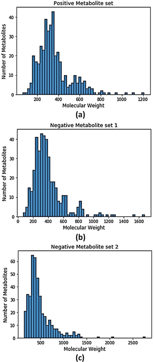
Histograms showing the frequency of metabolites in the context of molecular weight.

For experiments, the training data set was created by joining the 70 % data from both positive and negative sets. The remaining 30 % from both sets were joined to create the test dataset. We downloaded the SDF file of those metabolites from PubChem and generated the 1024 bit molecular fingerprint (The Morgan fingerprint) using the python RDkit package (Version 2017.09.02). The Morgan fingerprint is the implementation of the extended connectivity fingerprint (ECFP) which represents molecular structures by means of circular atom neighborhoods. ^[50] Each atom in a molecule is represented as a unique identifier and all possible paths of this molecule in the atom are explored by considering the circular radius. The paths are expressed in bit values by means of the identifiers and hash function.[ ⁵¹ , ⁵² ] The Morgan fingerprint is a powerful variant of Extended‐connectivity fingerprints (ECFPs) which is explicitly designed to capture molecular features relevant to molecular activity.^[50][54] ECFPs is widely used in similarity searching, clustering, and virtual screening. This fingerprint is also well suited for predicting and gaining insight into drug activity. ^[55] We use deep learning NN models in our experiments and present our work by following DOME ^[56] recommendations. Deep Learning is a feed forward artificial neural network that uses more than one hidden layer to capture the complex relationship among input variables.[ ⁵⁷ , ⁵⁸ ] In order to solve the overfitting problem, ^[59] this model can have white decay, sparsity, or dropout layers. Like other neural networks, DNN uses the weights, biases, nonlinear activation, and backpropagation to model the function defined by the input and output sets. Due to the multiple hidden layers in DNN, sparse multivariate polynomials data are exponentially easier to approximate compared to shallow NN. ^[60] Depending on feature selection, we utilized three different deep learning NN models in this work.

We explain the procedure of these models using dataset 1 and the final result shows the performance for both datasets.

2.1. Simple Fingerprint Model (SFM)

This is a simple model without any modification of input feature by feature reduction techniques. The model was created with 1024 input nodes equivalent to the number of fingerprints of individual metabolites. We consider this model as a simple benchmark to compare the performance of our second and third models. The training data are split into equal size batches. Each batch contains fingerprints of 50 metabolites and their corresponding antibacterial properties.

As the number of input features is much higher than binary output, we created the sequential neural network with two hidden layers. The first hidden layer contains 64 nodes and the second hidden layer contains 8 nodes. This requires a large number of weight variables to be tuned. One of the challenges of a neural network is controlling overfitting when the training dataset is insufficient comparing the weight variables of the model. ^[61] We used two dropout layers to reduce the overfitting. One is in between the input layer and the first hidden layer, and another one is in between the first hidden layer and the second hidden layer.

Drop out is a stochastic regularization technique to remove some nodes from DNN. Thus the contribution of those nodes on the activation function is fully omitted on forward pass. The weight update is not applied during the gradient calculation on backward pass. This technique repeats in each mini batch data on training period hence the sampling of thin networks happens from the large network. The optimum gradient calculation from a thin network will be a lot easier than a large network. Thus the weight and bias values tuned separately from a set of thin networks can reduce overfitting. The dropout ratio is measured by using the Bernoulli distribution. The probability p is considered as selection criteria from the node set of the hidden layer. p=1 means no dropout and p=0 means no output from the layer. Usually, the good value for p in a hidden layer is considered to be between 0.5 and 0.8. In our case, we used p=0.5 as the dropout ratio for both dropout layers.

The activation function Relu is used in each layer due to its less computational effort and better convergence performance. ^[53] The Binary Cross‐Entropy loss function with the mean reduction method is used to calculate the output variant. If x_i is input and y_i is the corresponding output from our model then cross‐entropy is measured by the following equation (Eq 1.

$${\displaystyle BCE=-\frac{1}{N}\sum _{i=1}^N{y}_i\log \left(p\left(y_i\right)\right)+\left(1-y_i\right)\log \left(1-p\left(y_i\right)\right)}$$ (1)

Here N is the number of input in each batch. p(y_i) is the predicted probability of the output being 1 and 1‐p(y_i) is the predicted probability of the output being 0 for a input.

The next two models also follow almost the same architecture of this model. All three NN models converged after around 100 epochs on training dataset. We fixed the number of epochs in every validation to 200.

2.2. Fingerprint Correlation Model (FCM)

In this model, we reduce some features based on collinearity. In the context of clustering and classification based on multivariate data, it is considered that highly correlated features contain very similar and/or redundant information. Therefore, to reduce some highly correlated features, we generated the binary relationship between fingerprints of all metabolites using Pearson correlation (Eq 2.

$${\displaystyle r=\frac{\sum (x_i-\bar{x})(y_i-\bar{y})}{\sqrt{\sum {(x_i-\bar{x})}^2\sum {(y_i-\bar{y})}^2}}}$$ (2)

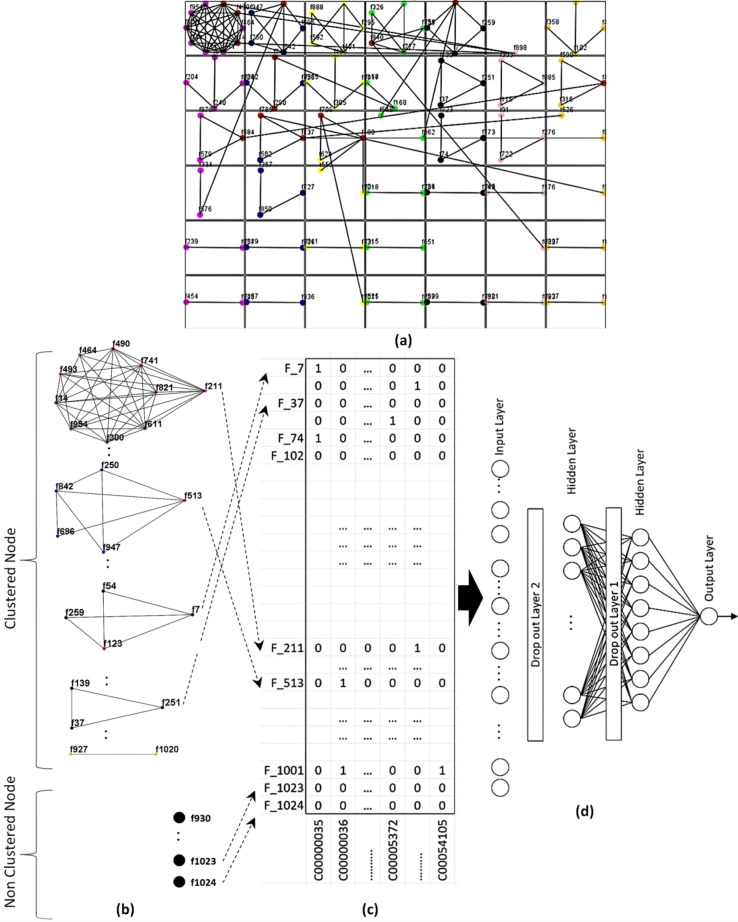
Here x_i and y_i are elemets of two fingerprint column vectors and $\bar{x}$ and $\bar{y}$ are the mean value of these vectors. r is the Pearson coefficient between the fingerprint columns. We determined the correlation between each pair of fingerprints and selected those pairs having a correlation value greater than 0.5. Thus we got only 138 pairs of relations comprising 116 fingerprints out of 1024 fingerprints from the dataset 1. These relations create a simple network where the nodes are the fingerprints. We applied the DPClusO algorithm to this network and created 42 overlapping clusters. For each cluster, we selected a significant node having the highest node degree within the cluster. The remaining nodes are discarded.

It is assumed that the significant node represents the best linear relationship in terms of Pearson coefficient to all other nodes within its own cluster. The isolated nodes which were not part of the cluster set were added to the feature set separately. The equation (Eq 3) shows the formation of the feature set using isolated nodes and significant nodes.

$${\displaystyle {\mathbf{S}}_{Total}=({\mathbf{S}}_{Fingerprint}\setminus {\mathbf{S}}_{Nnode})\cup {\mathbf{S}}_{SNode}}$$ (3)

Here S _Total =Set of all significant clustered nodes and non‐clustered nodes.

S _SNode =Set of significant nodes from the clusters.

S _Fingerprint =Set of fingerprints.

S _Nnode =Set of fingerprints in the network.

We used two hidden layers and two dropout layers same as to first NN model. We got total 950 features using | S _SNode |=42, | S _Fingerprint |=1024 and | S _Nnode |=116.

The workflow of this model is shown in Figure 2. The cluster set is drawn in Figure 2(a). Figure 2(b) shows all clusters with isolated nodes. The significant nodes are separately shown.

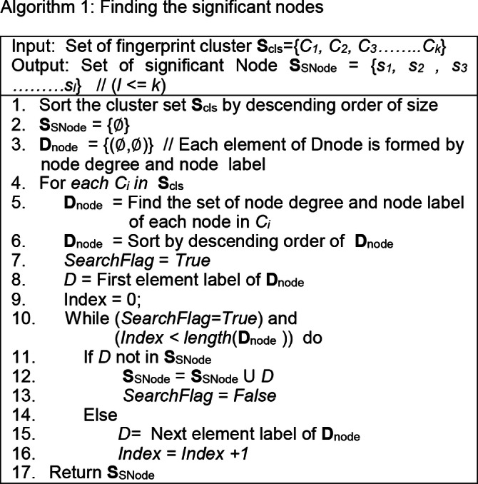
Figure 2.

a) Fingerprint clusters b) Significant nodes of clusters and non‐cluster nodes c) Mapping metabolites to significant nodes d) DNN.

In some cases, any overlapping node can be the significant node to more than one cluster. We consider this node as the significant node for the biggest cluster among its corresponding clusters. For the remaining clusters, the significant nodes are selected by the next highest node degree basis. The procedure is followed repeatedly until a significant node is found. Algorithm 1 explains the detailed process of finding significant nodes. If all elements of any small cluster are chosen to be the significant nodes by previous iteration then the cluster is omitted. In such a case, the number of elements in the set of the significant node is less than the number of clusters. The matrix of the fingerprints and metabolites is shown in Figure 2(c) after mapping the metabolites to the significant nodes. This model contains 950 input nodes and the rest of the architecture is similar to the first model.

2.3. Metabolites Cluster Model (MCM)

In this model, we generated the clusters of the metabolites based on their features (in the present case the fingerprints are the features) and utilized such clusters to find the representative metabolites to be included in the training data. We created a simple network where the metabolites are the nodes and the edges represent high structural similarity between the corresponding metabolites. Tanimoto coefficient was used to measure structural similarity between two metabolites. We added an edge between a pair of metabolites if the Tanimoto similarity between them is more than 0.85. We applied the DPClusO algorithm to this network and made an overlapping cluster set.

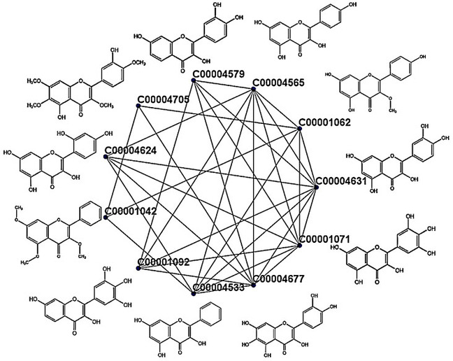
A typical cluster generated from dataset 1 is shown in Figure 3 with their molecular formula. The cluster contains 11 metabolites where eight of them are reported in our database with antibacterial properties.

Figure 3.

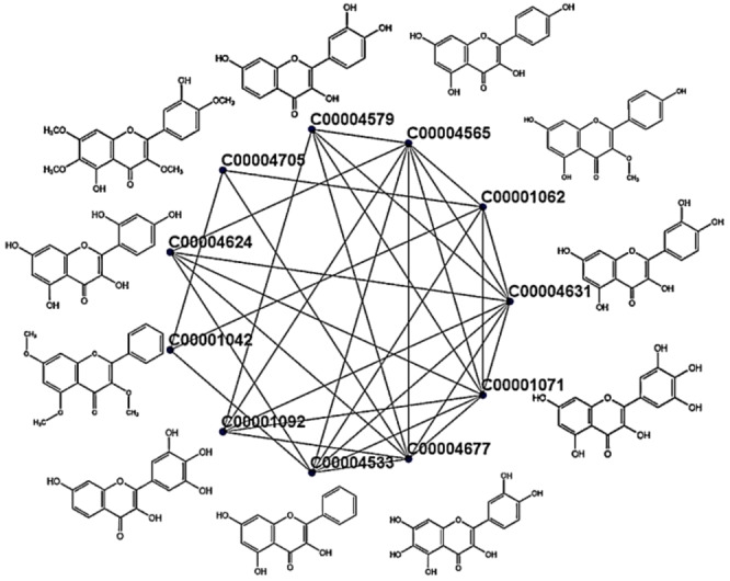
One simple cluster rendered from the cluster set of metabolites using DPClusOST.

These eight are Myricetin (C00001071), Plant: Machilus bombycina; Robinetin (C00001092), Plant: Robinia pseudoacacia; 3,5,7‐Trihydroxy‐2‐phenyl‐4H‐1‐benzopyran‐4‐one (C00004533), Plant: Nothofagus spp; Kaempferol (C00004565), Plant: Sapium sebifenum; 3,3′,4′,7‐Tetrahydroxyflavone (C00004579), Plant: Acacia peuce; Morin (C00004624), Plant: Machilus bombycina; Quercetin (C00004631), Plant: Cordia macleodii; Quercetagetin (C00004677), Plant: Tagetes patula. Except for some cases, each cluster contains almost similar structured metabolites. Some of the metabolites which remain isolated due to inadequate relation with other metabolites are considered as single node clusters.

Let the set of the metabolites is denoted by S _Metabolite ={m₁,m₂,m₃…….m_n } and the cluster set is denoted by S _cls ={C₁, C₂, C₃………C_k } where (k<n) and Ci ⊂ S _Metabolite .

The minimum number of metabolites in a cluster is 2. We applied the algorithm 1 to find out the significant node in each cluster.

If the significant nodes are denoted by S _SNode ={s₁, s₂, s₃ ……s_l } where (l≤k) then a portion of training dataset is formed by S _SNode . The set of isolated nodes or non‐clustered nodes can be denoted by following equation (Eq 4

$${\displaystyle {\mathbf{S}}_{noncls}={\mathbf{S}}_{Metabolite}\setminus \left\{C_1\cup C_2\cup C_3\cdots \cdots \cup C_k\right\}}$$ (4)

The remaining portion of the training dataset is formed from S _noncls set.

By intuition, we can realize that the more imbalanced clusters i. e. where the number of antibacterial and non‐antibacterial metabolites are largely unequal are likely to provide better representative for training data. In most cases, it is usual to have an unequal number of antibacterial and non‐antibacterial metabolites in each cluster. In the following theorem, we show that the probability of finding balanced clusters is indeed less than or equal to 0.5.

Theorem 1: If a binary dataset contains an equal number of positive and negative data then the probability is≤0.5 that a cluster formed by random selection contains an equal number of positive and negative data.

Proof: Let the dataset contain 2n number of data with n number of positive and n number of negative elements and a cluster c is formed where numbers of positive and negative elements are r and s respectively.

If the cluster c consists of odd number of elements, then the cluster has an unequal number of positive and negative data.

If the cluster c consists of even number of elements, then probability that c is balanced i. e.

$${\displaystyle \mathrm{P}\left(\mathrm{r}=\mathrm{s}\right)=\frac{\left(\begin{array}{c}\mathrm{n}\\ \mathrm{r}\end{array}\right)\left(\begin{array}{c}\mathrm{n}\\ \mathrm{s}\end{array}\right)}{\left(\begin{array}{c}2\mathrm{n}\\ \mathrm{r}+\mathrm{s}\end{array}\right)}=\frac{\left(\begin{array}{c}\mathrm{n}\\ \mathrm{r}\end{array}\right)\left(\begin{array}{c}\mathrm{n}\\ \mathrm{r}\end{array}\right)}{\left(\begin{array}{c}2\mathrm{n}\\ 2\mathrm{r}\end{array}\right)}=\frac{{\left(\begin{array}{c}\mathrm{n}\\ \mathrm{r}\end{array}\right)}^2}{\left(\begin{array}{c}2\mathrm{n}\\ 2\mathrm{r}\end{array}\right)}\left(\mathrm{Since}\mathrm{r}=\mathrm{s}\right)}$$ (5)

In our case n=412 and the above probability for r=1, 2, 3, 4, 10 are 0.50, 0.37, 0.31, 0.27, 0.17 respectively (very low). In fact, for a smaller increase in r and n the denominator increases at higher rate lowering the probability (proved).

Usually, clustering is done not by random selection but based on cohesive properties of the elements. Hence in general it is more likely that most of the generated clusters will be very imbalanced and thus will be more effective features for classification.

In the present case, the bigger portion of most clusters is formed by cohesive properties of either antibacterial or non‐antibacterial metabolites. Hence the significant node corresponding to a cluster has more chance to represent the bigger portion of the cluster. From Figure 3, three metabolites (C00001062, C00001042, and C00004705) do not have antibacterial property. These three metabolites have a weak relationship (smaller node degree) to the other eight antibacterial metabolites.

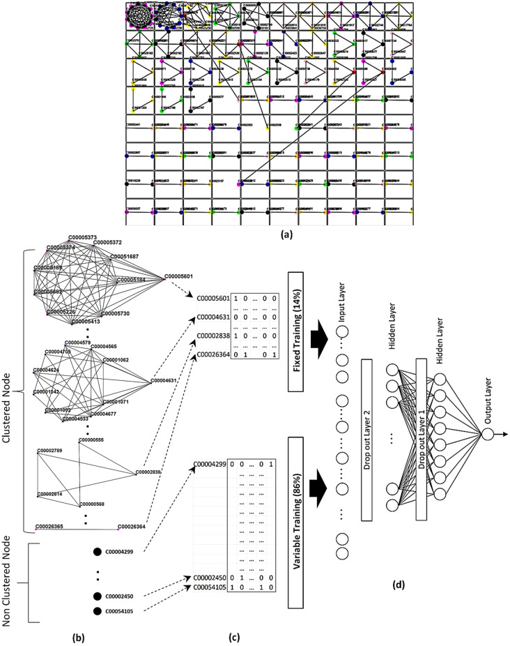
Due to the overlapping properties of clusters, the number of significant nodes can be smaller than the number of clusters. We got a total of 80 clusters comprising 226 distinct nodes by using the DPClusO algorithm from dataset 1. The remaining 598 metabolites did not form any cluster. After applying algorithm 1 in our cluster set, we got 79 distinct significant nodes out of 80 clusters. These 79 significant nodes are fixed in the training dataset which is 13 % of total training data. The rest of the training data (remaining 87 % of total training data) is randomly selected from 598 metabolites. The flow diagram is shown in Figure 4. All clusters drawn by the DPClusOST graph clustering tool are shown by descending order of their size in Figure 4(a). ^[46] The overlapping nodes are indicated by red color. As an example, the metabolite C0004631 and C0026364 are significant nodes on the cluster no 2 and 80. These two are shown in Figure 4(c) as a fixed part of the training set. Figure 4(b) shows the remaining portion of the training data formed by some of the metabolites from 598 non‐clustered metabolites. Finally, the matrix is inputted into the model. From Figure 4(d), the number of input nodes is 1024 and the output node is 1 in the model. First hidden layer contains 64 nodes and the second hidden layer contains 8 nodes.

Figure 4.

a) Metabolite clusters b) Significant nodes of clusters and non‐cluster nodes c) Mapping metabolites to fixed training and variable training d) DNN.

3. Results and Discussion

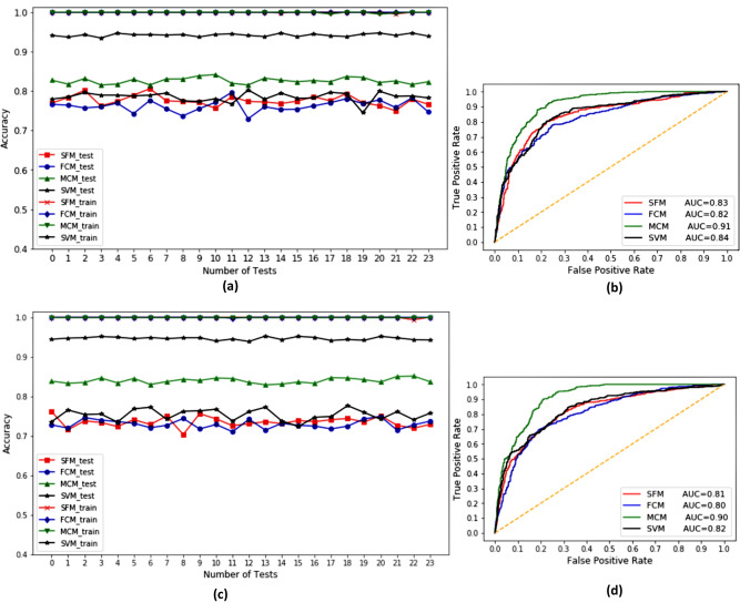
Each model is run multiple times by randomly creating the training data and test data. Only for the metabolite cluster model (MCM model), the training data are selected semi‐randomly. A SVM (Support Vector Machine) model is also created and finally all results are compared. Figure 5(a),(c) shows the prediction performance of the training and test data on twenty four different runs. Table 2 shows the performance metrics of the four models on the dataset 1 and dataset 2. The MCM approach offers the best performance (82.60 %, 83.94 %) on the test datasets. SFM and reduction of fingerprint features by clustering method i.e FCM both shows almost similar performance on test dataset (77.58 %, 76.22 % for dataset 1, 73.48 %, 72.91 % for dataset 2).

Figure 5.

Performance of different methods on training data and test data (dataset 1 (a), dataset 2 (c) ) ROC curves (dataset 1 (b), dataset 2 (d))

Table 2.

Average Performance of different models.

Methods	Features	Feature Reduction (%)	Accuracy (%)	ROC AUC (%)	Sensitivity (%)	Specificity (%)
Data set 1
MCM	1024	0	82.60±0.77	91.01±0.17	93.11±0.23	73.44±0.42
FCM	950	7.2	76.22±1.51	82.45±0.53	77.01±0.59	72.63±0.70
SFM	1024	0	77.58±1.32	83.23±0.39	77.98±0.17	76.05±0.19
SVM	1024	0	78.05±1.21	84.23±1.10	77.03±1.10	79.47±0.24

Data set 2
MCM	1024	0	83.94±0.65	90.81±0.17	89.91±0.14	78.54±1.02
FCM	926	9.5	72.91±1.09	80.15±1.01	74.18±0.59	73.17±0.61
SFM	1024	0	73.48±1.29	81.35±1.12	73.98±0.15	74.68±1.20
SVM	1024	0	75.35±1.42	82.39±0.51	75.40±1.03	77.43±0.27

± value indicates the standard deviation.

The maximum amount of feature reduction is obtained in the FCM (7.2 % on dataset 1, 9.5 % on dataset 2). ROC curves from Figure 5(b),(d) also show the high sensitivity on the MCM approach. SVM approach shows the best specificity on dataset 1 and MCM approach shows the best specificity on dataset 2. From our two datasets of 824 metabolites each, half of the metabolites are antibacterial compounds which formed a significant portion (67 clusters on dataset 1, 65 clusters on dataset 2) of the cluster set on MCM method. 13 clusters on dataset 1, 38 clusters on dataset 2 are formed by non‐antibacterial compounds which are mostly small clusters implying the presence of various different types of structures in the negative set.

The diversity of the data is basically formed by the non‐cluster behavior of metabolites which is adapted by SFM method on training. In our experiment of the MCM method, each metabolite of diverse physicochemical properties forms a single isolated cluster. The cluster with at least two metabolites has similar physiochemical properties which may have a contingent relationship to the antibacterial properties. This model selects the training data by taking the representative element from a group of similar types of metabolites. The representative elements contain only a small portion of training data and the rest large portion of training data are taken from non‐clustered metabolites. Thus it utilizes wider variety of data during the training period. Hence MCM method shows the best performance on the test dataset. On the other hand, the FCM method only reduces the redundant features which are linearly codependent. This method emphasizes the minimization of features on the input side without considering the relation of features with the output. The FCM method extracts the unique features which cover the maximum variance in the dataset. Due to this fact, the prediction performance is almost similar to the simple fingerprint method. MCM method proposed in this work is a somewhat new approach for training set development.

In the context of this approach, this can be stated that combining similar physicochemical properties using the graph clustering method before the machine learning approach can be an improved technique to predict the antibacterial activity. Using structure‐based clusters provided good classification results for test data in this work which directly implies that structure has good relation with activities in the case of chemical compounds. A cluster consisting of both negative and positive data contains the points near the class boundaries. When a high degree member from such a cluster is added to training data, then it is likely that the developed model will correctly classify the majority of the data points near the boundary corresponding to that cluster. If such clusters are good samples of background data, the model developed by the proposed method is likely to perform well also for classifying the unknown new data. For developing a good model, it is necessary that the selected training data contain representative members from across the distribution of all available data. Usually it is accomplished by random selection of training data. Our clustering approach will deterministically improve the diversity/variance of the training data and thus help develop a good model. Actually because of overfitting of a model, test data points near the class boundary are likely to be misclassified. Our approach somehow reduces that effect by allowing majority group near boundary to go to the correct class. It is noteworthy that this new approach of developing training data using clusters of entities themselves created based on important properties can help to avoid overfitting and cover wider variance/diversity in training data.

4. Conclusion

Antibacterial resistance and Infectious diseases are great threats to humans and leading causes of death worldwide. A large number of secondary metabolites from plant domain have been discovered whose activities are still unknown. The importance of those metabolites in agriculture, ecology, and healthcare is increasing. Availability of plant metabolomics data enables us to search for new antibacterial metabolites by the synergistic effort of machine learning and biochemical assays. The computational methods are less time‐consuming and less costly. Therefore, computational methods can be applied first to short list the candidates which can then be verified by biochemical assays. We have developed an SVM and three DNN models to predict the antibacterial ability of metabolites and compared the performance of these models. One of the important parts of a machine learning model development is to provide a good training data set by capturing the maximum variance. We found that combining machine learning with graph clustering to reshape the training data boosts the prediction performance. Biochemical experiment is the conclusive evidence to judge the antimicrobial properties of metabolites. Our model can be a precursor before detection of antibacterial properties of metabolites by expensive and complex biochemical experiments.

Author Contribution Statement

Mohammad Bozlul Karim and Md. Altaf‐Ul‐Amin designed the research and conducted the experiments. Shigehiko Kanaya guided the research with valuable comments. All authors have read and approved the final manuscript.

Conflict of interest

None declared.

M. B. Karim, S. Kanaya, M. Altaf-Ul-Amin, Mol. Inf. 2022, 41, 2100247.

Data Availability Statement

The data that support the findings of this study are available from the corresponding author upon reasonable request.

References

- 1. Amor I. L., Boubaker J., Sgaier M. B., Skandrani I., Bhouri W., Neffati A., Kilani S., Bouhlel I., Ghedira K., Chekir-Ghedira L., J. Ethnopharmacol. 2009, 125, 183–202. [DOI] [PubMed] [Google Scholar]
- 2. Compean K. L., Ynalvez R. A., Res. J. Med. Plant. 2014, 8, 204–213. [Google Scholar]
- 3. Savoia D., Future Microbiol. 2012, 7, 979–990. [DOI] [PubMed] [Google Scholar]
- 4. Rahman M. in Evidence-Based Validation of Herbal Medicine, 1st ed., Elsevier Science, 2015, pp. 495—513. [Google Scholar]
- 5. Gould I. M., Bal A. M., Virulence. 2013, 4, 185–191. [DOI] [PMC free article] [PubMed] [Google Scholar]
- 6.F .R. McSorley, J. W. Johnson, G. D. Wright, Antimicrobial. Resistance. 21st. Century. 2018, pp. 533–562.
- 7. Sengupta S., Chattopadhyay M. K., Grossart H. P., Front. Microbiol. 2013, 4, 47. [DOI] [PMC free article] [PubMed] [Google Scholar]
- 8. Viswanathan V. K., Gut. Microbes. 2014, 5, 3—4 . [DOI] [PMC free article] [PubMed] [Google Scholar]
- 9.Centers for Disease Control and Prevention, Office of Infectious Disease Antibiotic resistance threats in the United States, 2013. Apr, 2013. Available at: http://www.cdc.gov/drugresistance/threat-report-2013. Accessed January 28, 2015.
- 10. Read A. F., Woods R. J., EMPH. 2014, 1, 147. [DOI] [PMC free article] [PubMed] [Google Scholar]
- 11. Lushniak B. D., Public. Health. Rep. 2014, 4, 314–316. [DOI] [PMC free article] [PubMed] [Google Scholar]
- 12. Gross M., R1063-R1065. 2013. [DOI] [PubMed] [Google Scholar]
- 13. Piddock L. J., Lancet. Infect. Diseases. 2012, 12, 249–253. [DOI] [PubMed] [Google Scholar]
- 14. Bartlett J. G., Gilbert D. N., Spellberg B., Clin. Infect. Dis. 2013, 56, 1445–1450. [DOI] [PubMed] [Google Scholar]
- 15. Michael C. A., Dominey-Howes D., Labbate M., Public. Health. Front. 2014, 2, 145. [DOI] [PMC free article] [PubMed] [Google Scholar]
- 16. Gould I. M, Int. J. Antimicrob. Agents. 2008, 32, S2-S9. [DOI] [PubMed] [Google Scholar]
- 17. Wise R., J. Antimicrob. Chemother. 2011, 66, 1939–1940. [DOI] [PubMed] [Google Scholar]
- 18. Fischbach M. A., Walsh C. T., Science. 2009, 325, 1089–1093. [DOI] [PMC free article] [PubMed] [Google Scholar]
- 19. Martínez J. L., Rojo F., Vila J., Future. Microbiol. 2011, 6, 605–607. [DOI] [PubMed] [Google Scholar]
- 20. Shimamura T., Zhao W. H., Hu Z. Q., Antiinfect. Agents. Med. Chem. 2007, 6, 57–62. [Google Scholar]
- 21. Qin R., Xiao K., Bin Li., Jiang W., Peng W., Zheng J., Zhou H., Int. J. Mol. Sci. 2014, 14, 1802–1821. [DOI] [PMC free article] [PubMed] [Google Scholar]
- 22. Kim H. W., Choi S. Y., Jang H. S., Ryu B., Sung S. H., Yang H., Sci. Rep. 2019, 9, 1–11. [DOI] [PMC free article] [PubMed] [Google Scholar]
- 23. Kloosterman A. M., Medema M. H., van Wezel G. P., Curr. Opin. Biotechnol. 2021, 69, 60–67. [DOI] [PubMed] [Google Scholar]
- 24. Li H. B., Wong C. C., Cheng K. W., Chen F., LWT. 2008, 41, 385–390. [Google Scholar]
- 25. Iacopini P., Baldi M., Storchi P., Sebastiani L., J. Food Compos. Anal. 2008, 21, 589–598. [Google Scholar]
- 26. Foster B. C., Foster M. S., Vandenhoek S., Krantis A., Budzinski J. W., Arnason J. T., Gallicano K. D., Choudri S., J. Pharm. Sci. 2001, 4, 176–184. [PubMed] [Google Scholar]
- 27. Romano J. D., Tatonetti N. P., Front. genet. 2019, 10, 368. [DOI] [PMC free article] [PubMed] [Google Scholar]
- 28. Zhang R., Li X., Zhang X., Qin H., Xiao W., Nat. Prod. Rep. 2021, 38, 346–361. [DOI] [PubMed] [Google Scholar]
- 29. Chen Y., Kirchmair J., Mol. Inform. 2020, 39, 2000171. [DOI] [PMC free article] [PubMed] [Google Scholar]
- 30. Crozier A., Jaganath A. B., Clifford M. N. in Plant secondary metabolites: Occurrence, structure and role in the human diet, 1st ed., Blackwell Publishing Ltd, 2006, pp.1–21. [Google Scholar]
- 31. Dudareva N., Klempien A., Muhlemann J. K., Kaplan I., New. Phytol. 2013. 198, 16–32. [DOI] [PubMed] [Google Scholar]
- 32. Wink M. in Annual plant reviews, 1st ed., Vol 40, John Wiley & Sons, Ltd, 2010, pp.1–19. [Google Scholar]
- 33. Zang Q., Mansouri K., Williams A. J., Judson R. S., Allen D. G., Casey W. M., Kleinstreuer N. C., J. Chem. Inf. Model. 2017, 57, 36–49. [DOI] [PMC free article] [PubMed] [Google Scholar]
- 34. Davis T. D., Gerry C. J., Tan D. S., ACS Chem. Biol. 2014, 9, 2535–2544. [DOI] [PMC free article] [PubMed] [Google Scholar]
- 35. Stokes J. M., Yang K., Swanson K., Jin W., Cubillos-Ruiz A., Donghia N. M., MacNair C. R., et al., Cell. 2020, 180, 688–702. [DOI] [PMC free article] [PubMed] [Google Scholar]
- 36. O'Shea R., Moser H. E., J. Med. Chem. 2008, 51, 2871–2878. [DOI] [PubMed] [Google Scholar]
- 37. Myint K. Z., Wang L., Tong Q., Xie X. Q., Mol. Pharm. 2021, 9, 2912–2923. [DOI] [PMC free article] [PubMed] [Google Scholar]
- 38. Lo Y. C., Rensi S. E., Torng W., Altman R. B., Drug Discov. 2018, 23, 1538–1546. [DOI] [PMC free article] [PubMed] [Google Scholar]
- 39. Wei J. N., Duvenaud D., Aspuru-Guzik A., ACS Cent. Sci. 2016. ,2, 725–732. [DOI] [PMC free article] [PubMed] [Google Scholar]
- 40. Karelson M., Lobanov V. S., Katritzky A.R., Chem. Rev. 1996, 96, 1027–1044. [DOI] [PubMed] [Google Scholar]
- 41. Tropsha A., Gramatica P., Gombar V. K., QSAR Comb. Sci. 2003, 22, 69–77. [Google Scholar]
- 42. Cereto-Massagué A., Ojeda M. J., Valls C., Mulero M., Garcia-Vallvé S., Pujadas G., Methods. 2015, 71, 58–63. [DOI] [PubMed] [Google Scholar]
- 43. Altaf-Ul-Amin M., Tsuji H., Kurokawa K., Asahi H., Shinbo Y., Kanaya S., J. Comput. Aided Chem. 2006, 7, 150–156 . [Google Scholar]
- 44. Altaf-Ul-Amin M., Shinbo Y., Mihara K., Kurokawa K., Kanaya S., BMC Bioinform. 2006, 7, 207. [DOI] [PMC free article] [PubMed] [Google Scholar]
- 45. Altaf-Ul-Amin M., Wada M., Kanaya S., Int. Sch. Res. Notices. 2012, 2012. [Google Scholar]
- 46. Karim M. B., Wakamatsu N., Altaf-Ul-Amin M., J. Comput. Aided Chem. 2017, 8, 76–93. [Google Scholar]
- 47. Nakamura Y., Mochamad Afendi F., Kawsar Parvin A., Ono N., Tanaka K., Hirai Morita A., Sato T., Sugiura T., Altaf-Ul-Amin M., Kanaya S., Plant Cell Physiol. 2014, 55, e7–e7. [DOI] [PubMed] [Google Scholar]
- 48. Afendi F. M., Ono N., Nakamura Y., Nakamura K., Darusman L. K., Kibinge N., Morita A. H., Tanaka K., Horai H., Altaf-Ul-Amin M., Kanaya S., Comput. Struct. Biotechnol. J. 2013, 4, e201301010. [DOI] [PMC free article] [PubMed] [Google Scholar]
- 49. Abdullah A. A., Altaf-Ul-Amin M., Ono N., Sato T., Sugiura T., Morita A. H., Katsuragi T., Muto A., Nishioka T., Kanaya S., Biomed Res. Int. 2015. . [DOI] [PMC free article] [PubMed] [Google Scholar]
- 50. Rogers D., Hahn M., J. Chem. Inf. Model. 2010, 50, 742–754. [DOI] [PubMed] [Google Scholar]
- 51. Hu Y., Lounkine E., Bajorath J., ChemMedChem. 2009, 4, 540–548. [DOI] [PubMed] [Google Scholar]
- 52. Glen R. C., Bender A., Arnby C. H., Carlsson L., Boyer S., Smith J., Idrugs. 2006, 9, 199–204. [PubMed] [Google Scholar]
- 53. Krizhevsky A., Sutskever I., Hinton G. E., Adv. Neural Inf. Process. Syst. 2012, 25, 1097–1105. [Google Scholar]
- 54. Kensert A., Alvarsson J., Norinder U., Spjuth O., J. Cheminformatics. 2018, 10, 1–10. [DOI] [PMC free article] [PubMed] [Google Scholar]
- 55. Xia X., Maliski E. G., Gallant P., Rogers D., J. Med. Chem. 2004, 47, 4463–4470. [DOI] [PubMed] [Google Scholar]
- 56. Walsh I., Fishman D., Garcia-Gasulla D., Titma T., Pollastri G., Harrow J., Psomopoulos F. E., Tosatto S. C., Nat. Methods. 2021, 1–6.33408396 [Google Scholar]
- 57. Bengio Y. in Learning deep architectures for AI, 1st ed., Vol 2, Now Publishers Inc, 2009, pp. 1–18. [Google Scholar]
- 58. Schmidhuber J., Neural Netw. 2015, 61, 85–117. [DOI] [PubMed] [Google Scholar]
- 59. Bengio Y., Boulanger-Lewandowski N., Pascanu R., ICASSP. 2013, 8624–8628. [Google Scholar]
- 60. Rolnick D., Tegmark M., arXiv preprint arXiv. 2017, 1705.05502 . [Google Scholar]
- 61. Srivastava N., Hinton G., Krizhevsky A., Sutskever I., Salakhutdinov R., J. Mach. Learn. Res. 2014, 15, 1929–1958. [Google Scholar]
Associated Data
This section collects any data citations, data availability statements, or supplementary materials included in this article.