Machine-Learning Rationalization and Prediction of Solid-State Synthesis Conditions

Abstract

There currently exist no quantitative methods to determine the appropriate conditions for solid-state synthesis. This not only hinders the experimental realization of novel materials but also complicates the interpretation and understanding of solid-state reaction mechanisms. Here, we demonstrate a machine-learning approach that predicts synthesis conditions using large solid-state synthesis data sets text-mined from scientific journal articles. Using feature importance ranking analysis, we discovered that optimal heating temperatures have strong correlations with the stability of precursor materials quantified using melting points and formation energies (ΔG_f, ΔH_f). In contrast, features derived from the thermodynamics of synthesis-related reactions did not directly correlate to the chosen heating temperatures. This correlation between optimal solid-state heating temperature and precursor stability extends Tamman’s rule from intermetallics to oxide systems, suggesting the importance of reaction kinetics in determining synthesis conditions. Heating times are shown to be strongly correlated with the chosen experimental procedures and instrument setups, which may be indicative of human bias in the data set. Using these predictive features, we constructed machine-learning models with good performance and general applicability to predict the conditions required to synthesize diverse chemical systems.

Introduction

While solid-state synthesis is the prevailing approach for making inorganic solids, the determination of synthesis conditions for new solids is mostly based on heuristics and human-acquired experiences, with no analytical predictive approaches.^1,2 Recent work has focused on rationalizing solid-state reaction pathways observed in in situ experiments³⁻⁷ by decomposing them into a sequence of phase evolution steps¹ that can be modeled using thermodynamic calculations.⁸⁻¹¹ To design synthesis routes for new materials, it is essential to understand why certain conditions are preferred and develop models for predicting these conditions for synthesis (e.g., temperature, time). While thermodynamic calculations have been used to rationalize synthesis conditions in specific chemical systems,^8,12 a synthesis condition predictor with broad applicability for general inorganic compounds is still elusive.

Here, we use statistical machine-learning (ML) methods to systematically learn and quantitatively evaluate synthesis condition predictors from a large set of experimental data. Such ML approaches require large, high-quality synthesis data sets covering many chemistries, which have only recently become available through the application of natural language processing (NLP) and information retrieval techniques on the large body of scientific literature.¹³⁻¹⁹ In this work, using the data set of over 30 000 text-mined solid-state synthesis reactions (denoted as the text-mined “recipes” or the TMR data set in this paper),¹⁶ we demonstrate an inductive ML approach that learns synthesis conditions from the knowledge parsed from the past literature.

The overall pipeline of our ML approach is shown in Figure 1. Data sets of synthesis conditions compiled from NLP/text-mined data sets are used to train ML models. Each synthesis reaction was represented using a set of human-designed features, which will be discussed in more detail in subsequent sections. Interpretable ML models were trained on this basis of features to predict two key solid-state synthesis conditions that must be specified for any reaction: heating temperature and heating time.

Figure 1.

Schematic of the ML methods developed in this work for predicting solid-state synthesis conditions.

Throughout this paper, the prediction of solid-state synthesis conditions is defined as regression (point estimations) of the two experimental condition variables—temperature and time. Several important assumptions have been made: (a) Good synthesizability is assumed;²⁰⁻²³ i.e., when a publication reports the synthesis of some material at a specified set of conditions, we assume that this reaction was successful. (b) Synthesis experiments are performed in a one-shot fashion; i.e., reactants react and form the target compound in a single heating step, such that a simple synthesis route of “mix and heat” would be sufficient. (c) The ML models predict the “optimal” synthesis conditions as implicitly defined by the consensus of training data.

Note that the above assumptions oversimplify the synthesis condition prediction problem. These assumptions are often violated in many cases of practical solid-state syntheses. For example, a simple one-shot reaction route can thermodynamically favor an impurity phase which can only be avoided by using a multistep synthesis with specific intermediate compounds;^11,24 solid-state syntheses are often performed with many more degrees of freedom, such as special heating schedules,^8,24 special mixing devices,²⁵ different sintering aids,²⁶ etc. Moreover, the heating atmosphere strongly affects target material formation by changing the chemical potentials of gas species.²⁷ ML models require sufficient and consistent data to draw statistically significant conclusions,^28,29 while the data set used in this work has too imbalanced distributions for these additional labels. For example, only <5% of the reactions in the TMR data set have nonair synthesis atmospheres. Therefore, the aforementioned conditions, although present in the TMR data set, are not predicted by the ML models in this work. Modeling of these factors may become possible as text-mined data sets become abundant in the future.³⁰

In this work, we considered 133 synthesis features describing four aspects of solid-state syntheses: (1) precursor properties, (2) composition of the target material, (3) reaction thermodynamics, and (4) experimental procedure setup. We ranked these features according to their predictive power using dominance importance (DI) analysis.³¹ The features were used to train linear and nonlinear (tree-based) regressors for synthesis heating temperature and time. For all models, we split the data set into reactions with carbonate precursors and reactions without carbonate reactions. This splitting is necessary because the release of CO₂ gas in carbonate precursor materials systematically shifts the reaction driving forces for this subset and, consequently, the coefficients of the related features in linear models. Grouping the data set into carbonate and noncarbonate reactions thus fits two sets of coefficients that account for this shift and improves the overall performance. We performed leave-one-out cross-validation (LOOCV) to diagnose model performance. We also used out-of-sample (OOS) evaluation on Pearson’s Crystal Data³² (another synthesis data set independently extracted from the literature, denoted as the PCD data set in this paper) to test model generalizability on unseen data sets. The detailed data preprocessing and model construction can be found in the Methods section.

Our ML results achieve a goodness-of-fit measured by R² ∼ 0.5–0.6 and mean absolute error (MAE) ∼ 140 °C for heating temperature prediction. To compare with, typical heating temperatures used in solid-state synthesis range from ∼500 °C to ∼1500 °C. For heating time prediction, the time variable is transformed into a new prediction variable representing reaction speed: t → log₁₀(1/t) . The goodness-of-fit for this new time variable is R² ∼ 0.3, and MAE is ∼0.3 log₁₀(h^–1) (e.g., if the predicted time is t, the MAE estimates a range of [10^–0.3·t, 10^0.3·t], or [0.5t, 2t]). Analysis of the model predictive power reveals that heating temperature prediction is dominated by precursor properties, which we hypothesize to be linked to reaction kinetics. Heating time prediction is dominated by experimental operations, which may be indicative of human selection bias. The ML methods developed and applied in this work provide a statistically rigorous approach toward learning robust synthesis predictors from large data sets mined from the scientific literature.

Results

Synthesis Feature Selection Using Dominance Analysis

In total, we created 133 features in four categories: (1) precursor properties—12 features calculated from melting points, standard enthalpy of formation ΔH_f^300K, and standard Gibbs free energy of formation ΔG_f of precursors; (2) composition of the target material—74 indicator variables representing the presence (1) or absence (0) of different chemical elements in the target compound; (3) reaction thermodynamics—33 descriptive features of the driving forces for synthesis-relevant reactions constructed by decomposing synthesis into multistep phase evolution paths using previously developed principles;^7,8 and (4) experiment-adjacent features—14 indicator variables representing whether certain devices, procedures, and/or additives were used in the synthesis procedure. See Methods for a more detailed description of how each of these classes of features was computed.

We first use DI analysis³¹ to rank the predictive power of these features. In DI analysis, one constructs many linear models that predict outcomes using subsets of features, called submodels. DI analysis then calculates the incremental effect of a feature f_i on submodels that do not use f_i in three different ways. The average partial dominance importance (APDI) value for f_i is computed as the average increase of model performance, measured by R², when f_i is added to any submodel that does not include f_i. In other words, APDI measures the averaged gain of predictive power by including a feature. Individual dominance importance (IDI) values are the R² of models trained using only one feature and quantify the predictive power of the features by themselves. Interactional dominance importance (IADI) values are the decrease of model R² when a feature is removed from the whole model that uses all features, therefore measuring the gain of predictive power by a feature over all other features. All three DI values are computed for both heating temperature and time prediction models and are shown in Figure 2. We split the data set into carbonate reactions (reactions with at least one carbonate precursor) and noncarbonate reactions (reactions with no carbonate precursors). This is necessary because these two subsets have dissimilar distributions of reaction thermodynamic driving forces, which must be separated to be modeled in linear regression.^33,34

Figure 2.

DI values and rankings of the top 15 synthesis features for heating temperature models (a and b) and heating time models (c and d). The data set is split into carbonate reactions (reactions with at least one carbonate precursor) (a and c) and noncarbonate reactions (reactions with no carbonate precursors) (b and d). Interactional DI (IADI): decrease of model R² when a feature is removed from the whole model that uses all features. Individual DI (IDI): R² of models trained using only one feature. Average partial DI (APDI): average R² increase when a feature is added to a submodel. Features are ordered according to the sum of all three DI values.

We first evaluate the predictive powers of the features by themselves, as demonstrated by the IDI values in Figure 2. For heating temperature prediction, Figure 2a,b shows that the IDI values of the average precursor melting points are significantly higher than those of other features. Average precursor melting points alone achieve R² ∼ 0.2–0.3 for heating temperature prediction. Other features, such as experimental Gibbs free energy of formation at standard conditions ΔG_f^300K and experimental enthalpy of formation at standard conditions ΔH_f of precursors, are also highly predictive features as measured by IDI. Note that precursor melting points, ΔG_f^300K, and ΔH_f are likely to be good proxy variables for precursor reactivity. The next set of predictive features as ranked by IDI are compositional indicator variables (e.g., indicating the presence/absence of Li, Mo, Bi, etc.). These features can be understood as chemistry-specific corrections to heating temperatures. Note that ML models aim to reduce prediction errors for the whole training data set, which is dominated by the elements that are characteristic of large application fields, such as Li (Li-ion batteries) and Ba (perovskite oxides). It is thus not surprising that these most frequently synthesized chemical systems appear at the top of the list in Figure 2a,b.

For heating time prediction, Figure 2c,d shows that the IDI of experiment-adjacent features (e.g., indicators of polycrystal synthesis, phosphors, and usage of ball-milling devices) completely outweigh precursor property features. This suggests that heating time is largely controlled by the desired applications (e.g., the need for dense pellets, small particles, single crystals, etc.) and experimental setups rather than reaction mechanisms. Meanwhile, compositional indicator variables still rank second after the experiment-adjacent features, again acting as chemistry-specific corrections.

The blue bars in Figure 2 are IADI values. IADI values measure the gain of predictive power by a feature over all other features. For heating temperature prediction, Figure 2a,b shows that IADI values are very small for most features. A low IADI value is usually due to high correlation among features, e.g., average precursor melting points and maximal precursor melting points. These high correlations suggest it is necessary to use feature selection to choose the strongest feature among highly correlated features, as will be discussed in the next section. Nevertheless, a few features have relatively higher IADI values, a sign that they bring unique extra information over all other features. For example, describing syntheses using the word “sintering” may suggest the experimenters actively chose higher heating temperatures. As a consequence, the experiment-adjacent feature of “sintering” has the highest IADI value for temperature prediction models.

The green bars in Figure 2 are APDI values. APDI values are the average R² increase of a feature to all submodels. Thus, APDI estimates the general usefulness of a feature. APDI and IDI values are therefore two important factors in ranking feature importance. For example, in Figure 2a, even though average precursor melting point and ΔG_f^300K both have high IDI values, ΔG_f has smaller APDI values and is less important because of correlation with alternative features. By ranking all features according to the summation of DI values, we are able to consistently select the most uniquely predictive features.

While, in general, synthesis temperature and time together determine the overall reaction kinetics, they are not ranked as top predictive features in Figure 2 when included as features to predict each other (also see Table S1). This seems contrary to the expectation that they would be strongly correlated because elevated temperatures can lead to faster reactions by promoting atomic diffusion. We hypothesize that the low correlation between time and temperature may be due to a variety of reasons: (1) As opposed to sampling many synthesis conditions for a specific chemical system, the TMR data set spans diverse chemistries. There are usually less than 5 reported syntheses for a majority (>60%) of the chemical systems, which is not enough to reveal a stronger correlation, and (2) The TMR data set is text-mined from journal articles in which synthesis conditions, especially synthesis time, are generally not optimized but are determined by other external factors, such as the desired applications or the researcher’s convenience. These external factors make the time variable more noisy and less correlated to temperature than it might be in a variationally constrained set of data (e.g., the collection of shortest times for each temperature)

To summarize, the overall rankings in Figure 2 suggest each prediction variable is dominated by two types of features. For heating temperature prediction, precursor material properties have the most feature importance, while compositional features act as secondary corrections. For heating time prediction, experiment-adjacent features dominate the prediction, while compositional features also provide secondary corrections. Contrary to the common application of decomposing synthesis reactions into multistep phase evolution paths using thermodynamic principles,^8,10−12Figure 2 shows that the phase evolution thermodynamic driving force features, developed using similar principles in this work, provide little predictive power for heating temperature and time. We hypothesize that this is due to the fact that the TMR data set contains only positive experimental results for which researchers actively optimize for reasonable reaction kinetics. Therefore, reaction driving forces are less useful as these features are more likely to indicate whether something is synthesizable (e.g., if reactions to form a target are thermodynamically spontaneous) rather than indicate at what conditions reactions may occur quickly. We will revisit this finding in more detail in the Discussion section.

Building and Interpreting Linear Regression Models

To build regression models, we start with linear regressors as baseline models because their good interpretability allows one to focus on feature engineering and decipher the relations between features and synthesis conditions. To balance between high predictive power and possible overfitting, we add features in the order of DI rankings and drop any feature that increases model Bayesian information criterion (BIC) values.²⁹ In total, four linear models (heating temperature and time prediction models for carbonate and noncarbonate reactions) were trained using weighted least-squares (WLS).²⁹ The scatter plots of the predicted synthesis conditions versus the reported conditions are shown in Figure 3a,b. For heating temperature prediction, the R² values of the models are 0.55 on carbonate reactions and 0.56 on noncarbonate reactions, while the MAE values are 134 and 147 °C, respectively. For heating time prediction, the R² values of the models are 0.31 on carbonate reactions and 0.33 on noncarbonate reactions, while the MAE values are 0.30 log₁₀(h^–1) and 0.32 log₁₀(h^–1), respectively. Because we predict the transformed time variable log₁₀(1/t), such MAE estimates that the time prediction is within range [10^–0.3·t, 10^0.3·t], or [0.5t, 2t] (e.g., for a 2 h experiment, the expected prediction range is 0.5–4 h). Note that these metrics are evaluated on training data. Thus, they may not reflect the model performance when applied on unseen data. We will perform cross validation and discuss the results in later sections.

Figure 3.

Regression result of linear models. The scatter plots show reported conditions vs predicted conditions for temperature prediction (a) and time prediction (b). Opacity of the markers indicates the weights of data points. Histograms of prediction errors are also shown.

In a linear regressor ŷ = ∑_iβ_ix_i, the feature coefficients β_i quantify how the regression target variable responds to unit changes of x_i. As a special case, when x_i ∈{0, 1} are indicator variables (e.g., compositional and experimental-adjacent features), β_i can be interpreted as additive effects on the prediction target variable when features x_i = 1. For all compositional features, the effects are shown in Figure 4a,b. Note that these values are relative to the “average” according to the training data set and must be interpreted in relative values. For example, if Li is present in the target compound, Figure 4a suggests the heating temperature will decrease by 360 °C on average for noncarbonate reactions. On the other hand, the presence of N will increase the heating temperature by 260 °C on average. Therefore, Figure 4a,b show maps that associate different chemistries with their effect on optimal synthesis conditions. Such maps can be used as empirical “synthesis rules” that are helpful for designing synthesis routes to new materials.

Figure 4.

Average effect of each chemical element to predicted heating temperatures (a) and times (b) in trained linear models. The values are coefficients of the corresponding features in the linear models, quantifying how much the predicted value changes relatively if a new chemical element is added to (or removed from) the synthesis.

The learned coefficients in Figure 4a,b are sparse because some elements appear only a few times or are even missing in the training data set, precluding a confident estimate of their effect (assessed by the p-values of the coefficients with a 5% significance level³⁵). In Figure 4, we observe more consistent compositional effects across similar element periods and groups for temperature predictions than for heating time predictions. The lack of correlation with compositional effects for time prediction matches the DI analysis result in Figure 2c,d, which suggests compositional features are less helpful for predicting heating time. Moreover, the compositional effects are less consistent between carbonate reactions and noncarbonate reactions for heating time prediction. These observations suggests the compositional effects are generally less reliable for heating time prediction and must be used with more caution.

Training and Cross-Validating Nonlinear Models

Having used DI analysis and linear models to probe the synthesis prediction features, we next aim to systematically cross-validate ML models to understand their generalizability or propensity for overfitting. Figure 5 shows the model performances versus the number of features, which characterize training R² and the LOOCV Pseudo-R² (a metric comparable to R², see Methods) scores of the linear models as more features are included in training. In Figure 5, features are added into the models in the order of DI value rankings. Figure 5 shows that both training and LOOCV scores increase quickly when the number of features is less than 10. This result is consistent with the DI values in Figure 2 as the first few features have the highest feature importance. The model performance continues to improve as we include all other features, although the marginal improvement decreases rapidly. The training and LOOCV curves for linear models exhibit very similar performances, suggesting that these linear models have little risk of overfitting.

Figure 5.

Model performance versus number of training features for both linear and nonlinear (gradient boosting tree regressor) models. The x-axis shows the number of features used. The features are added in the order of DI value rankings. The first row shows performances of temperature prediction models trained on carbonate reactions (a) and noncarbonate reactions (b). The second row shows performances of time prediction models trained on reactions with (c) and without (d) carbonate precursors.

The linear model may be incapable of capturing nonlinear correlations among features and synthesis conditions. We next use advanced ML models that are capable of modeling nonlinear relations on the same set of features as for the linear models. Among the many ML models we attempted during preliminary experiments, gradient boosted regression trees (GBRT), implemented in the XGBoost package,³⁶ demonstrated the best LOOCV scores after proper hyperparameter tuning. XGBoost models use a large number of weak tree learners to build a strong ensemble regressor and are able to learn nonlinear effects. Indeed, we observe in Figure 5 that XGBoost training Pseudo-R² (red dashed curves) results are significantly higher than linear model results. However, as shown by the teal crosses in Figure 5, compared to the LOOCV scores of linear models (green stars), the LOOCV Pseudo-R² scores of XGBoost models do not improve as much when compared to the LOOCV performance of the linear models, suggesting an increased level of overfitting by XGBoost models. One advantage of XGBoost over linear models is improved utilization of a small number of features, as shown by the steeper curves when the number of features is less than 10 in Figure 5a,b, although the advantage diminishes once sufficiently many features are used. Finally, to help better understand the uncertainties of the models, we visualize the error distributions of synthesis conditions in Figure 6 using violin plots, where we mark the interquartile range (IQR) representing 50% of the errors, and 1.5x IQR, representing the range of prediction errors beyond which the errors are considered outliers.

Figure 6.

LOOCV prediction error distributions of synthesis temperature and time. Plotted are prediction error median values (shown with white dots), interquartile ranges (IQR, or the spread of errors between 25% and 75% percentiles, shown with thick lines), and 1.5× IQR (shown with thin lines). Shaded areas are probabilistic density estimations of the errors. Our models are expected to make prediction errors within the IQR approximately half of the time and within 1.5× IQR most of the time.

Testing Model Generalizability Using the PCD Data Set

When applied to unseen data sets, ML model predictions tend to have larger errors due to data set shift; i.e., unseen data sets have a different distribution than the training data sets.³⁷ In particular, the relations between features and outcomes may change for unseen data, leading to concept drift, degrading model generalizability and limiting model applicability.

The TMR data set mostly contains syntheses for inorganic oxide materials and is dominated by target materials containing Ti, Sr, Li, Ba, La, Nb, Fe, etc., reflecting popular materials in the inorganic materials research community such as perovskite oxides and battery materials. The TMR data set also contains a large fraction of solid solutions or doped materials. To estimate and understand how the ML models trained on the TMR data set generalize to unseen data sets, we utilized the PCD data set as an additional test. The original PCD collection contains inorganic materials syntheses that were manually extracted from the literature in a semistructured natural language form.³² We processed the PCD (Pearson’s Crystal Data) collection using the same text-mining pipeline and only kept oxide syntheses such that the final PCD data set has a similar chemistry distribution as the TMR data set. To ensure there are no duplicate syntheses, we removed any entry in the PCD data set whose digital object identifier (DOI) is present in the TMR data set (i.e., syntheses in the same papers are not allowed, but the same compositions from different papers are allowed). Compared to the TMR data set, the PCD data set shares a similar distribution of chemical systems and synthesis conditions, as indicated by similar sets of popular chemical elements (i.e., Ti, Fe, Sr, Ba, Si, etc.) and average synthesis temperatures around 1200 °C; see Figure S3. The PCD data set thus represents a reasonable benchmark data set for our ML models. However, because many reactions in the PCD data set do not have heating times extracted, we only predicted heating temperatures for the PCD data set.

To establish an upper bound of the model performance, we performed the same training/validation procedure using the PCD data set as was used on the TMR data set. Figure 7 shows the performance of the ML models versus the number of features. The green stars and teal crosses in Figure 7 are the LOOCV scores of linear and XGBoost models, respectively. XGBoost models achieve 0.5–0.6 LOOCV Pseudo-R² values which is considerably better than linear models (0.4–0.5). Moreover, XGBoost shows a steeper performance increase when few synthesis features are used. Compared to Figure 5, the advantage of the nonlinear models is much more substantial for the PCD data set than for the TMR data set. This clear advantage of XGBoost models indicates they are more robust than linear models against possible data set shift effects.

Figure 7.

Performance of the models versus the number of features evaluated on the PCD data set. X-axes show the number of features used in each model. Features are added in the order of DI value rankings as in Figure 2. The left panels (a) and (c) show models trained on carbonate reactions, and the right panels (b) and (d) show models trained on noncarbonate reactions. The top panels (a) and (b) show the performance of models trained and evaluated on the PCD data set, which represent the upper bounds of OOS scores (c) and (d), which show performance of the models trained on the TMR data set. A higher OOS score indicates better model generalizability.

Next, we performed tests to understand how well ML models trained on the TMR data set are generalizable to the PCD data set. The purple diamonds and yellow-brown triangles in Figure 7 show the OOS performances of the linear and XGBoost models trained using the TMR data set but evaluated on the PCD data set. It is interesting to note that XGBoost and linear models have very similar OOS scores for carbonate reactions, but XGBoost clearly outperforms linear models for noncarbonate reactions when more (>30) features are used. Upon further investigation, the features #30 to #40 used on noncarbonate reactions are mostly related to thermodynamic properties of the reactions. The performance drop after feature #30 suggests that relations between thermodynamic features and heating temperatures learned on the TMR data set by linear models do not transfer well to the PCD data set. On the other hand, XGBoost models seem to be able to consistently maintain good performance regardless of the number of features used.

In Figure 7, the difference between LOOCV scores and OOS scores confirms the ML models have degraded prediction performance (R² drops by 0.1) when applied to a different data set. The performance degradation caused by the data set shift is often inevitable and requires regularly retraining the ML models in order to adapt to the new data sets. However, Figure 7 suggests XGBoost models are more robust against the data set shift and have a better generalizability. We hypothesize this is due to the strong regularization and therefore recommend ML synthesis condition predictors to be built with XGBoost or similarly regularized models.

Discussion

ML predictions must be statistically evaluated using large data sets, so this work has focused heavily on reducing the expected prediction errors and improving the coefficient of determination R². We do not optimize models for any particular reaction but aim at predicting the synthesis conditions over a data set of several thousand synthesis reactions. As demonstrated by the cross-validation and OOS evaluations in Figure 5 and Figure 7, our models achieve R² ∼ 0.5–0.6 (MAE ∼ 140 °C) for heating temperature predictions and R² ∼ 0.3 (MAE ∼ 0.3 log₁₀(h^–1)) for heating time predictions. When evaluating these R² values, it is important to consider that heating temperature and time do not have a single value for a synthesis reaction, as compounds can often be synthesized over a broad range of times and temperatures. As such, our models may be more successful at predicting reaction conditions that successfully created the target, as surmised from the R² scores.

On the basis of the ranking of DI values in Figure 2, the deciding factors for the synthesis conditions can be organized into a two-level hierarchy. Synthesis temperature prediction is dominated by precursor properties, which we speculate are proxies for reactivity stemming from the mobility of ions, with additional corrections learned for different chemistries. Synthesis time prediction is dominated by experiment-adjacent features that are linked to experimental setups/intentions, also with corrections according to chemistry. The features used in this work to account for reaction thermodynamics were inspired by recent efforts to understand phase evolution during synthesis.^7−9,12,38 These features involve decomposing overall synthesis reactions into a sequence of phase evolution reactions between pairs of compounds and quantifying the grand potential thermodynamic driving force for these phase evolution reactions. This approach has proved especially useful for understanding phase evolution pathways observed in in situ experiments. However, in this work, they are shown to provide little predictive power of synthesis conditions and even cause the models to generalize poorly on OOS data sets (as demonstrated in Figure 7). This discrepancy will be discussed in more detail in the subsequent sections.

Synthesis Adjacent Information

We use the particular synthesis of BaTiO₃ from BaCO₃ and TiO₂ precursors to demonstrate how ML models combine synthesis adjacent information with the other regressors. BaTiO₃ is a popular compound with many applications in materials science and appears more than 100 times as the synthesis target in the TMR data set. A variety of synthesis temperatures have been reported for BaTiO₃ in the literature. For example, BaTiO₃ has been synthesized at 1000 °C,³⁹ 1100 °C,⁴⁰ 1200 °C,⁴¹ 1300 °C,⁴² and 1400 °C.⁴³ Here we focus on the effect of how many heating steps are used in the synthesis of BaTiO₃. Figure 8 shows the distribution of heating temperatures for all the reactions, BaTiO₃ with a single heating step, and BaTiO₃ with multiple heating steps in the training data set. It is clear that the reported heating temperatures with a single heating step have a lower center around 1100 °C (for example, see ref (40)), while the entries with multiple heating steps have a higher center around 1300–1400 °C (for example, see ref (43)).

Figure 8.

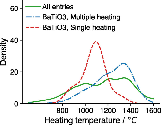
Curves are the estimated distribution of heating temperatures for each group of reactions in the training data set. The dashed/dotted lines show temperature distributions for the reaction TiO₂ + BaCO₃ → BaTiO₃ + CO₂ (red dashed line for single-heating reactions and blue dotted line for multiple-heating reactions). Green solid line shows the temperature distribution for the entire data set.

As a result, adding the target composition and experiment-adjacent features allows ML models to identify different groups of data as in Figure 8 and optimize the predicted heating temperature within each group. For example, if 0 means single heating and 1 means multiple heating, then the ML model should have a coefficient for the feature of “is multiple heating” of about 250 °C, roughly equal to the difference between the centers of the two temperatures distributions in Figure 8.

Connection to Tamman’s Rule

Our finding that the average precursor melting point is the most predictive feature for heating temperatures is reminiscent of Tamman’s rule.^44,45 Tammans rule can be formulated as predicting that the synthesis temperature of metal alloys should be more than 1/3 (for example, 1/2–2/3) of the precursor melting points. This rule is derived from the observation that atomic diffusion quickly ceases below 1/3 of melting temperatures.⁴⁶ Tamman’s empirical rule was never formally defined. It is also questionable whether the rule is applicable to the synthesis of ionic compounds (e.g., oxides) in addition to intermetallics. Nevertheless, variants of Tamman’s rule are still used to help determine solid-state synthesis conditions. For example, Becker and Dronskowski⁴⁷ used 2/3 of the most “volatile” compound;⁴⁷ other values, such as 1/2, have also been used.⁴⁵

Our ML framework allows us to formally model and test Tamman’s rule within a statistical approach. We start with Tamman’s original formulation and fit a linear model without an intercept term:

where T_Tamman is the predicted heating temperature, (minT_melt) is the minimum of precursor melting points, α is a parameter to be learned, and ε is an error term. Both the prediction and the melting points are presented in degrees Kelvin. The fit linear model finds α = 1.2 when trained on carbonate reactions and α = 0.8 when trained on noncarbonate reactions. These α values are larger than the commonly used values for Tamman’s rule, such as 1/2 and 2/3, suggesting the required temperatures for atoms to diffuse significantly in ionic compounds are higher than in intermetallics or that for ionic compounds Tamman’s rule is a surrogate for a property other than diffusion.

The above linear model is not the model with the highest predictive power (R² values). As shown in Figure 2, using average precursor melting points (instead of minimum precursor melting points) yields the highest prediction performance. Therefore, we update Tamman’s rule to give the optimal synthesis temperature T_Tamman as proportional to the average of precursor melting points (avgT_melt) plus a constant. Mathematically, the predictor is defined as

where α and β are parameters to be learned and ε is an error term.

As demonstrated in Figure 9, fitting a linear model reveals a slope of ∼1/3. Because we used the average of precursor melting points, the predicted heating temperatures should be generally larger than 1/3 of the minimal precursor melting point, agreeing with Tamman’s original observation.⁴⁴ The predicted versus reported heating temperatures and the histogram of prediction errors are shown in Figure 9a. The parameters of the fitted linear model are shown in Figure 9b. The large F-statistic values and very small p-values show strong statistical significance of the model, although this is contrasted by the low coefficient of determination (R² ∼ 0.2–0.3). Tamman’s rule is not a perfect predictor and has larger prediction errors at low temperatures. However, it contributes more than 1/3 of the maximal predictive power developed in this work.

Figure 9.

Fitting result of Tamman’s rule, i.e., synthesis temperature is proportional to the average precursor melting point. (a) Scatter plot of the reported vs predicted synthesis temperatures and histogram of prediction error. Opacity indicates data point weights. (b) Regression parameters and F-test for model significance. A very small p-value indicates that it is extremely unlikely the result is due to random noise.

Roles of Phase Evolution Reaction Analysis in Synthesis Condition Prediction

Predicting heating temperature is of major scientific interest. In solid-state synthesis, the final products are more sensitive to the heating temperature than time, because insufficiently low or high temperatures lead to incomplete reactions, impurities, or the complete absence of a desired target phase. Thus, heating temperatures are more carefully optimized than heating times, which are often chosen for convenience (e.g., to run overnight). There have been many successful examples where solid-state synthesis pathways are rationalized using the thermodynamics of reactions occurring during heating. For example, thermodynamic driving forces have been used to understand and control phase evolution pathways in Y–Mn–O oxides,^12,38 Y–Ba–Cu–O superconductors,⁸ Na–Co–O layered oxides,⁷ and MgCr₂S₄ thiospinel compounds.⁹ Inspired by this work, we computed features as numerical transformations of the thermodynamic driving forces obtained by decomposing the synthesis into multistep phase evolution paths. Contrary to the success in reconciling experimental observations in the aforementioned systems, these features are shown to provide no observable predictive powers for general synthesis condition predictions in this work (as shown in Figure 2 and Figure 7).

A low contribution of predictive power does not necessarily negate the effectiveness of phase evolution reaction analysis for understanding solid-state synthesis. It simply suggests that the features developed in this work are not correlated with the synthesis time and temperature over the diverse data sets evaluated in this work. We hypothesize this arises for a few reasons. First, the scale of the reaction driving force may dictate the decision boundary of synthesizable/nonsynthesizable conditions (e.g., synthesis should not occur at temperatures where the target phase is unstable with respect to decomposition). However, the data set used here only contains positive experimental results, so the thermodynamic stability of the target under the chosen synthesis conditions is likely already achieved for all data points. Indeed, in the rationalization of in situ synthesis, thermodynamic analysis has been used more to explain the phases observed along the reaction path rather than the specific conditions.^7,8,38 Second, once we are in the region of synthesizable conditions, the reaction driving force might become insufficient in determining synthesis conditions that lead to “fast” reactions. Because a typical lab synthesis needs to be completed in a reasonable period of time, experimenters may decide to raise heating temperatures to facilitate better reaction rates. Indeed, if we calculate the temperature T_equilibrium at which the reaction driving force is zero for the overall synthesis reaction (using the grand potential, ΔΦ_rxn = 0) for all the reactions, we found that this theoretical lower bound of heating temperatures T_equilibrium is generally much lower than the reported experimental T_exp. This suggests experimenters actively use T_exp ≫ T_equilibrium to achieve better kinetics. Unfortunately, reaction driving force analyses do not directly provide kinetic information, which is also chemistry-specific. On the other hand, precursor melting points and formation energies (ΔG_f^300K, ΔH_f) may be correlated to ion transport kinetics, as they are indicative of the relative strength of bonds in the solid precursors. This may explain why precursor material properties are the top predictive features for heating temperatures.

Previously, we demonstrated that precursor melting points (akin to Tamman’s rule) provide the most predictive power for heating temperatures if only one feature is allowed (see IDI values in Figure 2). We note here that the effectiveness of Tamman’s rule may also be due to the aforementioned selection bias⁴⁸ toward fast solid-state syntheses (as well as community knowledge of Tamman’s rule). This selection bias is inherent in the synthesis data set used in this work as the literature only reports “fast” and successful solid-state reactions. We note that some recent investigations of solid-state synthesis mechanisms^8,49 have put more emphasis on modeling reaction speeds. In addition, with the recent developments of autonomous synthesis robots,⁵⁰⁻⁵³ data on synthesizability and reaction speeds could be collected at the same time with a much higher throughput. Such data will be valuable for decorrelating selection bias and developing broadly applicable synthesis condition predictors.

Challenges of Predicting Synthesis Conditions Using Text-Mined Data

The performance of the ML models in this work is reasonable, but there is still much room for improvements to expand their applicability in practical synthesis design efforts. As potential improvements in the future, we summarize a few important aspects for increasing model performance.

Better Synthesis Features

Features are limiting factors in creating ML models with high predictive power. This work used 133 features spanning four categories: precursor material properties, target material compositions, reaction thermodynamics, and experiment-adjacent features. Besides these features, one set of useful features may be further factors that indicate the intention of syntheses. For example, the application for which the target compound is created (battery materials vs thermoelectric materials), desired microstructure of the target material morphology (single-crystal or spin-coated materials), etc. may all play a role in the determination of synthesis conditions. These features are expressed in papers in more subtle ways and could be potentially text-mined using advanced NLP techniques in the future.^54,55

Improved NLP Data Collection

As a result of the probabilistic nature of the text-mining pipeline that extracted the data sets in this work, errors in the training data are inevitable.¹⁶ Manual inspection reveals that 5% of heating temperatures and 16% of heating times were incorrectly extracted. Improved text-mining algorithms can thus improve data quality and increase ML model performance.

Modeling Nonuniqueness

In this work, we modeled synthesis condition predictions as point value regression problems. However, this may be suboptimal, as the conditions where a given synthesis can proceed are nonunique and often span a range of values. Consequently, there is not a unique ground truth of optimal synthesis conditions, which brings irreducible error to ML models. The issue of nonuniqueness is even more problematic for heating time prediction. If the synthesis finishes within t₀, then any heating time t > t₀ will yield the desired compound, if it is thermodynamically stable at the synthesis conditions and no selective evaporation of elements occurs. As a result, heating time is seldom optimized but based heavily on furnace heating schedule, lab shifts, etc. Indeed, in Figure 5, our ML models have larger errors for predicting heating time than for predicting heating temperature.

Modeling synthesis conditions as distributions, e.g., generalized linear models,⁵⁶ could in principle solve this issue. Note that sufficient training samples must be collected to get accurate condition distribution estimations (as well as uncertainties). Ideally, there would be several conditions sampled for each target that was synthesized in the data set. However, in the TMR data set, even when expanding the search to chemical systems (any targets having the same set of elements), more than 60% contain less than 5 reported syntheses. Furthermore, the distribution learned from the TMR data set may be biased by external factors. For example, for popular Li-ion cathode/anode materials in our data set, the distribution of different synthesis conditions may be correlated with the desired microstructure for a particular electrochemical performance. Decorrelating these factors requires mining of other features/properties beyond the synthesis reactions themselves.

Negative Samples

Negative experimental results are rarely reported in papers. Nevertheless, from an ML point of view, negative data are extremely useful for learning the exact decision boundaries of synthesis conditions. Besides, negative data can be used in other classification tasks, such as predicting the type of synthesis techniques, heating atmospheres, etc.

Finally, we note that the models in this work focused primarily on oxides, which make up a substantial fraction of inorganic compounds but not all.⁵⁷ Transferring predictive models trained on oxides to other chemistries is challenging because of significant concept drift. For example, the bonding of other types of compounds, such as nonoxide chalcogenides and intermetallics, is fundamentally different than that of oxides, leading to different self-diffusion and interdiffusion rates. This difference modifies the distributions of feature values significantly (e.g., melting points are systematically lower for metal precursors compared to oxides). If simply applied to other chemistries without any retraining, the parameters fit for oxide compounds would systematically mis-predict the synthesis conditions. However, if sufficient data becomes available for desired nonoxide materials classes of interest, the methods used in this work would be useful for training and interpreting these new models.

Conclusion

In this work, we developed an interpretable ML method for predicting solid-state synthesis heating temperatures and times on over 6300 synthesis reactions, which are from a larger (over 30 000) synthesis data set text-mined from scientific literature.¹⁶ The goodness-of-fit values are R² ∼ 0.5–0.6 for temperature prediction and R² ∼ 0.3 for time prediction. However, interpretation of such R² values has to consider the fact that there is no single exact time or temperature for a typical synthesis. For heating temperature prediction, which is an important parameter for solid-state synthesis, the prediction MAE of our model is ∼140 °C, comparable to a similar study using generative conditional variational autoencoder (CVAE).¹⁹ Heating time prediction has an MAE of ∼0.3 log₁₀(h^–1), which translates to a prediction range [0.5t, 2t] if the predicted time is t. The expected prediction errors can be estimated from Figure 6.

Analysis of the ML models reveals that melting points and formation energies of precursors are good predictors for heating temperatures, which led us to extend Tamman’s rule from intermetallics to oxide compounds for predicting heating temperatures as linearly proportional to the average precursor melting point. One may use this extended Tamman’s rule to set quick, yet reasonable, initial heating temperatures for new solid-state reactions. The maps of compositional effects (Figure 4) can be further used as guides to choose synthesis conditions with better accuracy given the chemistries of interest. Our model was trained and validated on a diverse set of materials and thus has broad applicability. Moreover, the ML methodologies developed in this work can be applied for learning synthesis conditions on other large synthesis data sets, such as solution-based synthesis of inorganic compounds and nanoparticles,^58,59 or even other tasks where strong model interpretability is preferred.

Methods

Curation of Synthesis Training Data

We used the data set of text-mined synthesis recipes that consists of 30 004 solid-state synthesis records¹⁶ to generate the TMR data set. We took the synthesis conditions of the last heating step in the experimental procedures as the target of prediction. The synthesis heating temperatures were predicted in degrees Celsius. The reported heating times were transformed to log₁₀(1/t), which is not only a better variable for measuring reaction speed but also shows smaller skewness and long-tailedness, which is better predicted by statistical ML models.²⁹ Note that the TMR data set is extracted using ML models and contains errors in synthesis conditions. On the basis of manual inspection, about 5% of the heating temperatures and 16% of the heating times were incorrectly extracted.

To preprocess the data set, we first removed all entries with no extracted synthesis heating temperatures and times. To obtain thermodynamic data for all targets, we utilized the Materials Project (MP) database.⁵⁷ For targets that appear as entries in MP, we simply used the reported thermodynamic information. For targets without a direct match to an MP entry, we performed interpolation by representing them using linear combinations of the most similar entries in MP as measured by the difference in composition (see Supporting Information for calculation details). The 0 K thermodynamic data was then transformed to finite-temperature Gibbs free energies of formation using the previously developed method.⁶⁰

Using the finite-temperature ΔG_f(T) predictions and thermodynamic properties of gases, we computed reaction driving forces, i.e., the grand potential change for the synthesis reactions, ΔΦ_rxn, by assuming the system is open to atmospheric partial pressures of O₂ and CO₂.⁶¹⁻⁶³ The reactions were then decomposed into phase evolution steps by selecting pairs of reactants with the largest grand potential change in each step. Details of the thermodynamic quantity calculation and phase evolution construction can be found in the Supporting Information and reproduced using the provided codes.

We removed the reactions that cannot be handled by the above thermodynamic calculations (e.g., missing relevant MP entries or containing gases other than O₂ and CO₂), leading to 7562 remaining reactions. As a result of the release of CO₂ gases in carbonate precursor materials, the reaction driving forces have systematically shifted distributions for reactions with and without carbonate precursors. Grouping the data set into carbonate and noncarbonate reactions thus fits two sets of coefficients that account for this shift and improves the overall performance. Therefore, in our analysis, we split the data set into carbonate reactions and noncarbonate reactions.

The original Pearson’s Crystal Data (PCD) collection is semistructured containing chemical formulas of input/output materials and a natural language description of the synthesis procedure. We used the same approach as in the generation of the TMR data set to balance synthesis reactions and calculate phase evolution reaction thermodynamic driving forces. The synthesis procedure description text is used to text-mine synthesis operations that contain synthesis condition values. To make the PCD data set have a chemistry distribution similar to that of the TMR data set, we only kept oxide syntheses as the TMR data set is dominated by oxide syntheses. We also ensured there are no duplicates by removing any entries in the PCD data set that are also in the TMR data set by matching their article DOIs.

Features for Synthesis Prediction

For each reaction in the curated training data, we computed four types of synthesis features (133 features in total).

Precursor Compound Properties

The first type of features (12 in total) are the average/minimum/maximum/difference of melting points, standard enthalpy of formation ΔH_f^300K, and standard Gibbs free energy of formation ΔG_f of the precursors. The melting points were retrieved from the NIST Chemistry WebBook⁶⁴ and PubChem databases,⁶⁵ while the thermodynamic properties were retrieved from the FREED database,⁶⁶ an electronic compilation of the U.S. Bureau of Mines (USBM) thermodynamic data obtained with experiment.

Target Compound Compositional Features

The second type of features are 74 indicator variables representing the presence (1) or absence (0) of different chemical elements in the target compound. We did not use more differentiating features such as the fractional compositions of each element because more than 60% of the chemical systems in the TMR data set have less than 5 samples, and more differentiating features make ML models prone to overfitting. Note that this may not be true if training data were to become relatively abundant for each chemical system, in which case numerical encoding of the compositions may be a better approach.

Reaction Thermodynamics Features

We used 33 thermodynamic features, including the total reaction driving force ΔΦ_rxn, first and last pairwise reaction driving forces ΔΦ_rxn,1 and ΔΦ_rxn,–1, and the ratio between first/last pairwise reaction driving force and the total reaction driving force, evaluated at different temperatures T = 800, 900, 1000, 1100, 1200, and 1300 °C. We also calculated the slopes of ΔΦ_rxn, ΔΦ_rxn,1, and ΔΦ_rxn,–1 by assuming they are linear with respect to temperature and used the slopes as additional features.

Experiment-Adjacent Features

The fourth type of features are 14 experiment-adjacent features, i.e., indicator variables representing whether certain devices (zirconia balls for ball-milling), experimental procedures (sintering, ball-milling, multiple heating steps, homogenization, repeated grinding, diameter measurement, polycrystalline preparation), and additives (binder materials, distilled water and other liquid additives, phosphors, poly(vinyl alcohol)) were used in the synthesis.

Because we used WLS, which is sensitive to outliers, we performed outlier detection algorithms on the feature values and removed around 10% of the reactions. The final training data consists of two data sets totaling 6325 reactions. The subset of carbonate reactions consists of 3182 reactions. The subset of noncarbonate reactions consists of 3143 reactions.

Training and Evaluation of ML Models

We used linear and nonlinear regressors to train the ML models. For linear models, we used WLS, a weighted version of ordinary least-squares in Python packages scikit-learn(67) and statsmodels.³⁵ For nonlinear models, we used the XGBoost package³⁶ and trained GBRT models. To evaluate the model goodness-of-fit, we used the coefficient of determination, R-squared (or R²). For nonlinear regressors and out-of-sample evaluations, R² is poorly defined, and Efron’s extended version⁶⁸ of Pseudo-R² was used. Pseudo-R² is calculated as 1 – (mean square error/variance of data) and directly comparable to R² values.

We implemented DI analysis, a model-agnostic method that calculates the average increase of model R² to rank features according to their contribution of predictive powers. Three types of DI values−APDI values, IDI values, and IADI values−were computed according to Azen and Budescu.³¹ However, to compute the exact APDI values for all 133 features, we needed to train 2¹³³ (sub)models, which is a computationally prohibitive task. Instead, we estimated APDI values as Δ(R²) by randomly sampling 200 submodels for each feature. All the features were ranked according to the sum of the APDI, IDI, and IADI values. This ranking measures the relative predictive powers of the features and was used to sort all features into an ordered list, as in Figure 2.

We next used the ranking of predictive power to perform forward feature selection for the ML models. Specifically, we started with a linear model with no features but the intercept term. Features were sequentially added into the linear model according to the ranking of predictive power. In this process, we calculated the BIC value of the linear models and removed any feature that would increase the BIC value (an indicator of overfitting). The final list of features were then used in training the models in Figures 5 and 7.

We performed LOOCV to cross-validate regressors and detect overfitting. To test model generalizability, we applied out-of-sample prediction by evaluating model performances on another synthesis condition data set compiled from the PCD data set.³²

Supporting Information Available

The Supporting Information is available free of charge at https://pubs.acs.org/doi/10.1021/acs.chemmater.2c01293.

• Further details about the calculation of synthesis predictive features and the construction of machine-learning models (PDF)

Author Present Address

^¶ Toyota Research Institute, 4440 El Camino Real, Los Altos, California 94022, United States

The authors declare no competing financial interest.

Notes

All codes and data needed to reproduce the results can be found at this repository: https://github.com/CederGroupHub/s4.

References

- Kohlmann H. Looking into the Black Box of Solid-State Synthesis. Eur. J. Inorg. Chem. 2019, 2019, 4174–4180. 10.1002/ejic.201900733. [DOI] [Google Scholar]
- Chamorro J. R.; McQueen T. M. Progress toward solid state synthesis by design. Accounts of chemical research 2018, 51, 2918–2925. 10.1021/acs.accounts.8b00382. [DOI] [PubMed] [Google Scholar]
- Shoemaker D. P.; Hu Y.-J.; Chung D. Y.; Halder G. J.; Chupas P. J.; Soderholm L.; Mitchell J.; Kanatzidis M. G. In situ studies of a platform for metastable inorganic crystal growth and materials discovery. Proc. Natl. Acad. Sci. U. S. A. 2014, 111, 10922–10927. 10.1073/pnas.1406211111. [DOI] [PMC free article] [PubMed] [Google Scholar]
- McClain R.; Malliakas C. D.; Shen J.; He J.; Wolverton C.; González G. B.; Kanatzidis M. G. Mechanistic insight of KBiQ2 (Q = S,Se) using panoramic synthesis towards synthesis-by-design. Chemical Science 2021, 12, 1378–1391. 10.1039/D0SC04562D. [DOI] [PMC free article] [PubMed] [Google Scholar]
- Ito H.; Shitara K.; Wang Y.; Fujii K.; Yashima M.; Goto Y.; Moriyoshi C.; Rosero-Navarro N. C.; Miura A.; Tadanaga K. Kinetically Stabilized Cation Arrangement in Li3YCl6 Superionic Conductor during Solid-State Reaction. Advanced Science 2021, 8, 2101413. 10.1002/advs.202101413. [DOI] [PMC free article] [PubMed] [Google Scholar]
- Paradis-Fortin L.; Lemoine P.; Prestipino C.; Kumar V. P.; Raveau B.; Nassif V.; Cordier S.; Guilmeau E. Time-resolved in situ neutron diffraction study of Cu22Fe8Ge4S32 germanite: a guide for the synthesis of complex chalcogenides. Chem. Mater. 2020, 32, 8993–9000. 10.1021/acs.chemmater.0c03219. [DOI] [Google Scholar]
- Bianchini M.; Wang J.; Clément R. J.; Ouyang B.; Xiao P.; Kitchaev D.; Shi T.; Zhang Y.; Wang Y.; Kim H.; et al. The interplay between thermodynamics and kinetics in the solid-state synthesis of layered oxides. Nature materials 2020, 19, 1088–1095. 10.1038/s41563-020-0688-6. [DOI] [PubMed] [Google Scholar]
- Miura A.; Bartel C. J.; Goto Y.; Mizuguchi Y.; Moriyoshi C.; Kuroiwa Y.; Wang Y.; Yaguchi T.; Shirai M.; Nagao M.; et al. Observing and Modeling the Sequential Pairwise Reactions that Drive Solid-State Ceramic Synthesis. Adv. Mater. 2021, 33, 2100312. 10.1002/adma.202100312. [DOI] [PubMed] [Google Scholar]
- Miura A.; Ito H.; Bartel C. J.; Sun W.; Rosero-Navarro N. C.; Tadanaga K.; Nakata H.; Maeda K.; Ceder G. Selective metathesis synthesis of MgCr2S4 by control of thermodynamic driving forces. Materials horizons 2020, 7, 1310–1316. 10.1039/C9MH01999E. [DOI] [Google Scholar]
- McDermott M. J.; Dwaraknath S. S.; Persson K. A. A graph-based network for predicting chemical reaction pathways in solid-state materials synthesis. Nat. Commun. 2021, 12, 3097. 10.1038/s41467-021-23339-x. [DOI] [PMC free article] [PubMed] [Google Scholar]
- Aykol M.; Montoya J. H.; Hummelshøj J. Rational solid-state synthesis routes for inorganic materials. J. Am. Chem. Soc. 2021, 143, 9244–9259. 10.1021/jacs.1c04888. [DOI] [PubMed] [Google Scholar]
- Wustrow A.; Huang G.; McDermott M. J.; O’Nolan D.; Liu C.-H.; Tran G. T.; McBride B. C.; Dwaraknath S. S.; Chapman K. W.; Billinge S. J.; et al. Lowering Ternary Oxide Synthesis Temperatures by Solid-State Cometathesis Reactions. Chem. Mater. 2021, 33, 3692–3701. 10.1021/acs.chemmater.1c00700. [DOI] [Google Scholar]
- Kim E.; Huang K.; Tomala A.; Matthews S.; Strubell E.; Saunders A.; McCallum A.; Olivetti E. Machine-learned and codified synthesis parameters of oxide materials. Scientific data 2017, 4, 170127. 10.1038/sdata.2017.127. [DOI] [PMC free article] [PubMed] [Google Scholar]
- Kim E.; Huang K.; Saunders A.; McCallum A.; Ceder G.; Olivetti E. Materials synthesis insights from scientific literature via text extraction and machine learning. Chem. Mater. 2017, 29, 9436–9444. 10.1021/acs.chemmater.7b03500. [DOI] [Google Scholar]
- Kim E.; Jensen Z.; van Grootel A.; Huang K.; Staib M.; Mysore S.; Chang H.-S.; Strubell E.; McCallum A.; Jegelka S.; et al. Inorganic materials synthesis planning with literature-trained neural networks. J. Chem. Inf. Model. 2020, 60, 1194–1201. 10.1021/acs.jcim.9b00995. [DOI] [PubMed] [Google Scholar]
- Kononova O.; Huo H.; He T.; Rong Z.; Botari T.; Sun W.; Tshitoyan V.; Ceder G. Text-mined dataset of inorganic materials synthesis recipes. Scientific data 2019, 6, 203. 10.1038/s41597-019-0224-1. [DOI] [PMC free article] [PubMed] [Google Scholar]
- Vaucher A. C.; Zipoli F.; Geluykens J.; Nair V. H.; Schwaller P.; Laino T. Automated extraction of chemical synthesis actions from experimental procedures. Nat. Commun. 2020, 11, 3601. 10.1038/s41467-020-17266-6. [DOI] [PMC free article] [PubMed] [Google Scholar]
- Young S. R.; Maksov A.; Ziatdinov M.; Cao Y.; Burch M.; Balachandran J.; Li L.; Somnath S.; Patton R. M.; Kalinin S. V.; et al. Data mining for better material synthesis: The case of pulsed laser deposition of complex oxides. J. Appl. Phys. 2018, 123, 115303. 10.1063/1.5009942. [DOI] [Google Scholar]
- Karpovich C.; Jensen Z.; Venugopal V.; Olivetti E.. Inorganic Synthesis Reaction Condition Prediction with Generative Machine Learning. arXiv, 2021-12-17, 2112.09612, https://arxiv.org/abs/2112.09612 (accessed 2022-07-16).
- Davariashtiyani A.; Kadkhodaie Z.; Kadkhodaei S. Predicting synthesizability of crystalline materials via deep learning. Communications Materials 2021, 2, 115. 10.1038/s43246-021-00219-x. [DOI] [Google Scholar]
- Sun W.; Powell-Palm M. J.. Generalized Gibbs’ Phase Rule. arXiv, 2021-05-04, 2105.01337, https://arxiv.org/abs/2105.01337 (accessed 2022-07-16).
- Sun W.; Dacek S. T.; Ong S. P.; Hautier G.; Jain A.; Richards W. D.; Gamst A. C.; Persson K. A.; Ceder G. The thermodynamic scale of inorganic crystalline metastability. Science advances 2016, 2, e1600225. 10.1126/sciadv.1600225. [DOI] [PMC free article] [PubMed] [Google Scholar]
- Aykol M.; Dwaraknath S. S.; Sun W.; Persson K. A. Thermodynamic limit for synthesis of metastable inorganic materials. Science advances 2018, 4, eaaq0148. 10.1126/sciadv.aaq0148. [DOI] [PMC free article] [PubMed] [Google Scholar]
- Dinia A.; Vénuat J.; Colis S.; Pourroy G. Elaboration and characterization of the Sr2FeMoO6 double perovskite. Catalysis today 2004, 89, 297–302. 10.1016/j.cattod.2003.12.019. [DOI] [Google Scholar]
- Shi T.; Xiao P.; Kwon D.-H.; Sai Gautam G.; Chakarawet K.; Kim H.; Bo S.-H.; Ceder G. Shear-assisted formation of cation-disordered rocksalt NaMO2 (M = Fe or Mn). Chem. Mater. 2018, 30, 8811–8821. 10.1021/acs.chemmater.8b03490. [DOI] [Google Scholar]
- Rao C. N. R.; Biswas K.. Essentials of inorganic materials synthesis; John Wiley & Sons: 2015. [Google Scholar]
- Yuan T.; Cai R.; Shao Z. Different effect of the atmospheres on the phase formation and performance of Li4Ti5O12 prepared from ball-milling-assisted solid-phase reaction with pristine and carbon-precoated TiO2 as starting materials. J. Phys. Chem. C 2011, 115, 4943–4952. 10.1021/jp111353e. [DOI] [Google Scholar]
- Montgomery D. C.; Peck E. A.; Vining G. G.. Introduction to linear regression analysis; John Wiley & Sons: 2021. [Google Scholar]
- Friedman J. H.The elements of statistical learning: Data mining, inference, and prediction; Springer: 2017. [Google Scholar]
- Kononova O.; He T.; Huo H.; Trewartha A.; Olivetti E. A.; Ceder G. Opportunities and challenges of text mining in materials research. iScience 2021, 24, 102155. 10.1016/j.isci.2021.102155. [DOI] [PMC free article] [PubMed] [Google Scholar]
- Azen R.; Budescu D. V. The dominance analysis approach for comparing predictors in multiple regression. Psychological methods 2003, 8, 129–148. 10.1037/1082-989X.8.2.129. [DOI] [PubMed] [Google Scholar]
- Villars P.; Cenzual K.. Pearson’s Crystal Data: Crystal Structure Database for Inorganic Compounds (on DVD), release 2021/22; ASM International: Materials Park, OH, U.S.A., 2021. [Google Scholar]
- Faria S.; Soromenho G. Fitting mixtures of linear regressions. Journal of Statistical Computation and Simulation 2010, 80, 201–225. 10.1080/00949650802590261. [DOI] [Google Scholar]
- Li Y.; Liang Y. Learning mixtures of linear regressions with nearly optimal complexity. Conf. Learning Theory 2018, 1125–1144. [Google Scholar]
- Seabold S.; Perktold J. Statsmodels: Econometric and Statistical Modeling with Python. Proc. 9th Python Sci. Conf. 2010, 92–96. [Google Scholar]
- Chen T.; Guestrin C. Xgboost: A scalable tree boosting system. Proceedings of the 22nd acm sigkdd international conference on knowledge discovery and data mining 2016, 785–794. 10.1145/2939672.2939785. [DOI] [Google Scholar]
- Quiñonero-Candela J.; Sugiyama M.; Lawrence N. D.; Schwaighofer A.. Dataset shift in machine learning; MIT Press: 2009. [Google Scholar]
- Todd P. K.; McDermott M. J.; Rom C. L.; Corrao A. A.; Denney J. J.; Dwaraknath S. S.; Khalifah P. G.; Persson K. A.; Neilson J. R. Selectivity in Yttrium Manganese Oxide Synthesis via Local Chemical Potentials in Hyperdimensional Phase Space. J. Am. Chem. Soc. 2021, 143, 15185–15194. 10.1021/jacs.1c06229. [DOI] [PubMed] [Google Scholar]
- Singh R.; Kaur J.; Bose P.; Shrivastava R.; Dubey V.; Parganiha Y. Intense visible light emission from dysprosium (Dy3+) doped barium titanate (BaTiO3) phosphor and its thermoluminescence study. Journal of Materials Science: Materials in Electronics 2017, 28, 13690–13697. 10.1007/s10854-017-7212-z. [DOI] [Google Scholar]
- Munakata F.; Yoshino K.; Nemoto K.; Abe S.; Ito A. Effect of self-assembly material texture and dielectric properties of BaTiO3/poly-l-lactic-acid composites. Mater. Lett. 2018, 221, 147–149. 10.1016/j.matlet.2018.03.008. [DOI] [Google Scholar]
- Alluri N. R.; Selvarajan S.; Chandrasekhar A.; Saravanakumar B.; Lee G. M.; Jeong J. H.; Kim S.-J. Worm structure piezoelectric energy harvester using ionotropic gelation of barium titanate-calcium alginate composite. Energy 2017, 118, 1146–1155. 10.1016/j.energy.2016.10.143. [DOI] [Google Scholar]
- Zheng S.; Ma X.; Yamamoto T.; Ikuhara Y. Atomistic study of abnormal grain growth structure in BaTiO3 by transmission electron microscopy and scanning transmission electron microscopy. Acta Mater. 2013, 61, 2298–2307. 10.1016/j.actamat.2012.12.046. [DOI] [Google Scholar]
- Zheng P.; Zhang J.; Tan Y.; Wang C. Grain-size effects on dielectric and piezoelectric properties of poled BaTiO3 ceramics. Acta Mater. 2012, 60, 5022–5030. 10.1016/j.actamat.2012.06.015. [DOI] [Google Scholar]
- Tammann G.Lehrbuch der Metallographie: Chemie und Physik der Metalle und ihrer Legierungen; Leopold Voss: Leipzig, 1932; p 314. [Google Scholar]
- Merkle R.; Maier J. On the tammann-rule. Zeitschrift für anorganische und allgemeine Chemie 2005, 631, 1163–1166. 10.1002/zaac.200400540. [DOI] [Google Scholar]
- The original German text by Tamman is “Die Zahl der Platzwechsel in der Zeiteinheit nimmt vom Schmelzpunkt an mit sinkender Temperatur schnell ab und wird bei Metallen bei Metallen bei 1/3 der absoluten Schmelztemperatur unmerklich.” This translates to “The number of changes of place in the unit of time decreases rapidly from the melting point with falling temperature and becomes imperceptible for metals at 1/3 of the absolute melting temperature.”
- Becker N.; Dronskowski R. A first-principles study on new high-pressure metastable polymorphs of MoO2. J. Solid State Chem. 2016, 237, 404–410. 10.1016/j.jssc.2016.03.002. [DOI] [Google Scholar]
- Berger V. W.; Christophi C. A. Randomization technique, allocation concealment, masking, and susceptibility of trials to selection bias. Journal of Modern Applied Statistical Methods 2003, 2, 80. 10.22237/jmasm/1051747680. [DOI] [Google Scholar]
- Cosby M. R.; Mattei G. S.; Wang Y.; Li Z.; Bechtold N.; Chapman K. W.; Khalifah P. G. Salt effects on Li-ion exchange kinetics of Na2Mg2P3O9N: Systematic in situ synchrotron diffraction studies. J. Phys. Chem. C 2020, 124, 6522–6527. 10.1021/acs.jpcc.0c00067. [DOI] [Google Scholar]
- Szymanski N. J.; Zeng Y.; Huo H.; Bartel C. J.; Kim H.; Ceder G. Toward autonomous design and synthesis of novel inorganic materials. Materials Horizons 2021, 8, 2169–2198. 10.1039/D1MH00495F. [DOI] [PubMed] [Google Scholar]
- Kimmig J.; Zechel S.; Schubert U. S. Digital Transformation in Materials Science: A Paradigm Change in Material’s Development. Adv. Mater. 2021, 33, 2004940. 10.1002/adma.202004940. [DOI] [PMC free article] [PubMed] [Google Scholar]
- Chen S.; Hou Y.; Chen H.; Tang X.; Langner S.; Li N.; Stubhan T.; Levchuk I.; Gu E.; Osvet A.; et al. Exploring the stability of novel wide bandgap perovskites by a robot based high throughput approach. Adv. Energy Mater. 2018, 8, 1701543. 10.1002/aenm.201701543. [DOI] [Google Scholar]
- Ortiz B. R.; Adamczyk J. M.; Gordiz K.; Braden T.; Toberer E. S. Towards the high-throughput synthesis of bulk materials: thermoelectric PbTe-PbSe-SnTe-SnSe alloys. Molecular Systems Design & Engineering 2019, 4, 407–420. 10.1039/C8ME00073E. [DOI] [Google Scholar]
- Weston L.; Tshitoyan V.; Dagdelen J.; Kononova O.; Trewartha A.; Persson K. A.; Ceder G.; Jain A. Named entity recognition and normalization applied to large-scale information extraction from the materials science literature. J. Chem. Inf. Model. 2019, 59, 3692–3702. 10.1021/acs.jcim.9b00470. [DOI] [PubMed] [Google Scholar]
- Trewartha A.; Walker N.; Huo H.; Lee S.; Cruse K.; Dagdelen J.; Dunn A.; Persson K. A.; Ceder G.; Jain A. Quantifying the advantage of domain-specific pre-training on named entity recognition tasks in materials science. Patterns 2022, 3, 100488. 10.1016/j.patter.2022.100488. [DOI] [PMC free article] [PubMed] [Google Scholar]
- Nelder J. A.; Wedderburn R. W. Generalized linear models. Journal of the Royal Statistical Society: Series A (General) 1972, 135, 370–384. 10.2307/2344614. [DOI] [Google Scholar]
- Jain A.; Ong S. P.; Hautier G.; Chen W.; Richards W. D.; Dacek S.; Cholia S.; Gunter D.; Skinner D.; Ceder G.; et al. Commentary: The Materials Project: A materials genome approach to accelerating materials innovation. APL materials 2013, 1, 011002. 10.1063/1.4812323. [DOI] [Google Scholar]
- Wang Z.; Kononova O.; Cruse K.; He T.; Huo H.; Fei Y.; Zeng Y.; Sun Y.; Cai Z.; Sun W.; et al. Dataset of solution-based inorganic materials synthesis procedures extracted from the scientific literature. Scientific Data 2022, 9, 231. 10.1038/s41597-022-01317-2. [DOI] [PMC free article] [PubMed] [Google Scholar]
- Cruse K.; Trewartha A.; Lee S.; Wang Z.; Huo H.; He T.; Kononova O.; Jain A.; Ceder G. Text-mined dataset of gold nanoparticle synthesis procedures, morphologies, and size entities. Scientific Data 2022, 9, 234. 10.1038/s41597-022-01321-6. [DOI] [PMC free article] [PubMed] [Google Scholar]
- Bartel C. J.; Millican S. L.; Deml A. M.; Rumptz J. R.; Tumas W.; Weimer A. W.; Lany S.; Stevanović V.; Musgrave C. B.; Holder A. M. Physical descriptor for the Gibbs energy of inorganic crystalline solids and temperature-dependent materials chemistry. Nat. Commun. 2018, 9, 4168. 10.1038/s41467-018-06682-4. [DOI] [PMC free article] [PubMed] [Google Scholar]
- Bartel C. J.; Trewartha A.; Wang Q.; Dunn A.; Jain A.; Ceder G. A critical examination of compound stability predictions from machine-learned formation energies. npj Computational Materials 2020, 6, 97. 10.1038/s41524-020-00362-y. [DOI] [Google Scholar]
- Bartel C. J.; Weimer A. W.; Lany S.; Musgrave C. B.; Holder A. M. The role of decomposition reactions in assessing first-principles predictions of solid stability. npj Computational Materials 2019, 5, 4. 10.1038/s41524-018-0143-2. [DOI] [Google Scholar]
- Bartel C. J. Review of computational approaches to predict the thermodynamic stability of inorganic solids. J. Mater. Sci. 2022, 57, 10475–10498. 10.1007/s10853-022-06915-4. [DOI] [Google Scholar]
- NIST Chemistry WebBook. https://webbook.NIST.gov/chemistry/ (accessed 2022-07-16).
- Kim S.; Chen J.; Cheng T.; Gindulyte A.; He J.; He S.; Li Q.; Shoemaker B. A.; Thiessen P. A.; Yu B.; et al. PubChem in 2021: new data content and improved web interfaces. Nucleic acids research 2021, 49, D1388–D1395. 10.1093/nar/gkaa971. [DOI] [PMC free article] [PubMed] [Google Scholar]
- FREED-Thermodynamic Database. https://www.thermart.net/freed-thermodynamic-database/ (accessed 2022-07-16).
- Pedregosa F.; et al. Scikit-learn: Machine Learning in Python. Journal of Machine Learning Research 2011, 12, 2825–2830. [Google Scholar]
- Efron B. Regression and ANOVA with zero-one data: Measures of residual variation. Journal of the American Statistical Association 1978, 73, 113–121. 10.1080/01621459.1978.10480013. [DOI] [Google Scholar]
Associated Data
This section collects any data citations, data availability statements, or supplementary materials included in this article.