Hierarchical Clustering and Target-Independent QSAR for Antileishmanial Oxazole and Oxadiazole Derivatives

Abstract

Leishmaniasis is a neglected tropical disease that kills more than 20,000 people each year. The chemotherapy available for the treatment of the disease is limited, and novel approaches to discover novel drugs are urgently needed. Herein, 2D- and 4D-quantitative structure–activity relationship (QSAR) models were developed for a series of oxazole and oxadiazole derivatives that are active against Leishmania infantum, the causative agent of visceral leishmaniasis. A clustering strategy based on structural similarity was applied with molecular fingerprints to divide the complete set of compounds into two groups. Hierarchical clustering was followed by the development of 2D- (R² = 0.90, R²pred = 0.82) and 4D-QSAR models (R² = 0.80, R²pred = 0.64), which showed improved statistical robustness and predictive ability.

1. Introduction

Visceral leishmaniasis (VL) is a neglected tropical disease (NTD) caused by the protozoan parasites Leishmania infantum and L. donovani and is the most severe form of leishmaniasis. Transmission occurs through the bite of infected female Phlebotominae sandflies. VL is a fatal disease if not treated and is the second leading cause of death among parasitic conditions after malaria. The disease has become a severe global health problem, with more than 200 million people currently at risk of infection worldwide [1]. The current treatments include drugs such as amphotericin B, sodium stibogluconate, miltefosine, and paromomycin, which present several drawbacks, including distribution and availability issues, long-term and complex treatment regimens, teratogenicity, toxicity, and drug resistance [2,3]. These shortcomings, combined with the high burden caused by the disease, highlight an urgent need for new treatment options for VL.

Despite the widespread use of the available drugs, little is known about their mechanisms of action, which reflects the main strategy that has been used for NTD drug discovery: phenotypic screening [4]. Despite the lack of information on the molecular targets, the phenotypic strategy is useful to account for activity against whole cells along with aspects of cell uptake, cytocidal or cytostatic mechanisms, and time-to-kill, among other relevant issues.

Therefore, the phenotypic approach has been widely used in drug discovery for NTDs given the very few validated molecular targets explored in the field [5,6].

Aligned with the strategy of phenotypic screening, the combination of different bioactive chemical scaffolds can be used to enrich the chemical diversity explored in NTD drug discovery. Recently, our group reported a hybridization approach combining two heterocyclic cores presenting antiparasitic activity, which guided the design of novel hybrid compounds with promising antileishmanial and anti-Trypanosoma cruzi activities [4]. One core is represented by oxadiazoles, and the other is 3-substituted 2-oxindoles, both of which are useful scaffolds, especially as antileishmanial agents [7,8,9,10,11].

The main goal of this work was the development of QSAR models using our in-house set of oxazoles and oxadiazoles that displayed in vitro antileishmanial activity against intracellular amastigotes. To this end, a computational approach using 2D- and 4D-QSAR strategies was conducted. Hierarchical clustering based on ligand structure was applied to split the dataset into two structurally similar groups. The integration of the experimental results with the applied ligand-based drug design studies (LBDD) yielded statistically significant QSAR models with the ability to predict the activity of new antileishmanial agents within a defined applicability domain.

2. Results and Discussion

2.1. AutoQSAR

The initial model was obtained considering the complete set of molecules using the AutoQSAR method. A set of seven binary fingerprints (dendritic, linear, atom pair, atom triplet, topological, MOLPRINT 2D, and radial) was generated to characterize the structures and create the 2D molecular descriptors. Different regression techniques, such as multiple linear regression (MLR), partial least squares regression (PLS), principal components regression (PCR), and kernel-based PLS (KPLS), were adopted to build the set of models. Random selection of the molecules for the test and training sets was applied using the AutoQSAR machine learning routine specifically designed for this end. All seven binary fingerprints available were used as molecular descriptors to build the 2D-QSAR models. The fingerprints and regression approaches were systematically combined to generate the best models, which are described in Table 1.

Table 1.

The most statistically significant models generated by AutoQSAR using the complete dataset.

Training Set (%)	R 2	SD	Q2 (R2pred)	RMSE	N	Fingerprint
70	0.5378	0.2180	0.4937	0.2123	1	Radial
75	0.5997	0.2065	0.5284	0.1994	2	Dendritic
80	0.6304	0.2022	0.6107	0.1817	5	MOLPRINT 2D

R²: coefficient of determination for the training set; SD: standard deviation; Q²: predictive correlation coefficient for the test set (R²_pred); RMSE: root-mean-square error for the test set predictions; N: optimum number of components.

For the complete dataset, the model that produced the best statistical parameters and score was obtained by the MOLPRINT2D binary fingerprint. The best regression method selected by the AutoQSAR routine was the KPLS technique with an 80:20 training/test set ratio, that is, 52 molecules in the training set and 13 compounds in the test set. This model yielded an R² value of 0.6304 and a Q² value of 0.6107.

Aiming to improve the predictive ability of the model, a structural analysis of the molecules in the dataset suggested that they have a diverse scaffold pattern. Therefore, to improve the QSAR results, hierarchical clustering was applied to the entire dataset.

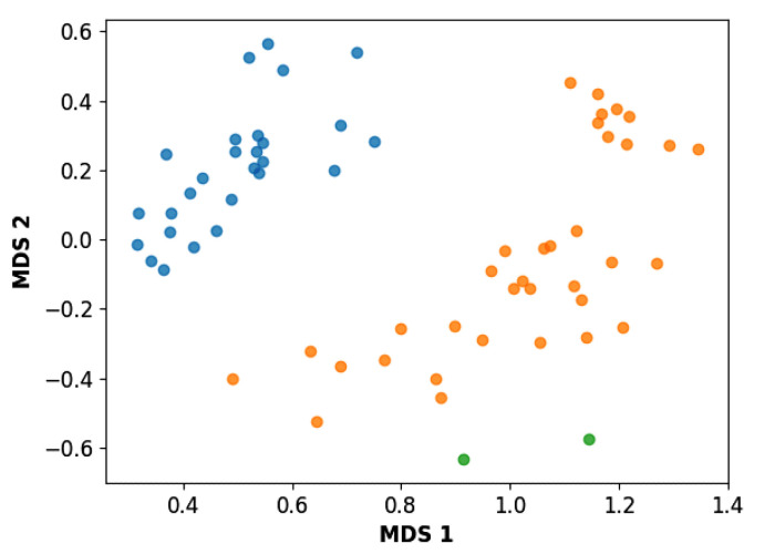
To start the hierarchical clustering analysis, the binary fingerprints (dendritic, linear, atom pair, atom triplet, topological, MOLPRINT 2D, and radial) were calculated for the entire set of molecules and used as molecular descriptors for this analysis. First, the Kelley level [12] was used to select the optimal number of clusters. In this step, a considerable number of singletons (clusters with one molecule) were obtained, which indicates the structural diversity in the dataset. The next step was the separation of the entire dataset into two groups. To separate these two groups according to the similarity between the molecules, the total number of clusters was divided to generate only two clusters which were as populous as possible; i.e., starting with the Kelley level, the number of clusters was reduced until the formation of two groups. These two groups of compounds were defined so that both groups included a considerable number of molecules to build the two QSAR models. This strategy resulted in the exclusion of two molecules that were identified as structural outliers [13,14]. As a result of this cluster analysis, the initial dataset originated two groups of compounds: the G₁ group with 27 compounds and the G₂ group with 35 compounds. The scaffolds of each group are presented in Figure 1. The structural diversity present in the dataset can be observed through the scatter plot obtained with the multidimensional scaling (MDS) plot illustrated in Figure 2. From each of these groups, two new and independent QSAR models were built.

Figure 1.

General scaffold of group G₁ (left) and group G₂ (right).

Figure 2.

Scatter plot obtained by multidimensional scaling (MDS). The molecules of the G₁ group are shown in blue, the molecules of the G₂ group are shown in orange, and the structural outliers are shown in green.

It is worth noting that group G₁ in Figure 1 and Figure 2 is less structurally diverse than group G₂. In Figure 2, the molecules of the G₁ group are more concentrated, while in the G₂ group, the molecules are more dispersed over the MDS plot. This structural diversity may have influenced the QSAR statistical parameters for each group, as the less diverse group (G₁) resulted in better statistical indicators.

For the G₁ group, the model that produced the best statistical parameters and score was represented by radial fingerprints and included 22 molecules in the training set and 5 in the test set (proportion 80:20). This is indicated by R² = 0.9069, SD = 0.1039, Q² = 0.8201, RMSE = 0.0945 and KPLS factor = 2. The best models for each training/test set split are shown in Table 2.

Table 2.

Statistically significant models generated by AutoQSAR for the G₁ group.

Training Set (%)	R 2	SD	Q2 (R2pred)	RMSE	N	Fingerprint
70	0.8982	0.1178	0.7132	0.1018	2	Radial
75	0.8012	0.1413	0.7022	0.1668	1	Radial
80	0.9069	0.1039	0.8201	0.0945	2	Radial

For the G₂ group, the model that produced the best statistical parameters was represented by dendritic fingerprints and included 28 molecules in the training set and 7 in the test set (proportion 80:20). This finding is indicated by R² = 0.8206, SD = 0.1377, Q² = 0.8001, RMSE = 0.1081 and KPLS factor = 3. The best models for each split are shown in Table 3.

Table 3.

Statistically significant models generated by AutoQSAR for the G₂ group.

Training Set (%)	R 2	SD	Q2 (R2pred)	RMSE	N	Fingerprint
70	0.6109	0.205	0.4206	0.1829	2	MOLPRINT 2D
75	0.5693	0.2040	0.5351	0.1041	2	MOLPRINT 2D
80	0.8206	0.1377	0.8001	0.1081	3	Dendritic

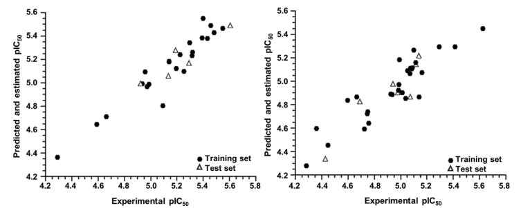
The predicted pIC₅₀ values obtained for both groups, G₁ and G₂, are represented graphically in Figure 3 along with the experimental pIC₅₀ values. Both plots show good agreement between the experimental and predicted activity for the AutoQSAR models. In addition, Table 4 shows the predicted and experimental pIC₅₀ values for the entire dataset (complete set model) and for the two groups of molecules obtained after the hierarchical cluster analysis (cluster model).

Figure 3.

Experimental versus predicted and estimated pIC₅₀ values for the training and test sets of the G₁ (left) and G₂ (right) groups.

Table 4.

Experimental, predicted, and residual values of pIC₅₀ for the G₁ and G₂ groups.

		2D-QSAR					4D-QSAR
		Complete Set Model			Cluster Model		Complete Set Model		Cluster Model
No.	pIC50 exp	pIC50 pred	Residue	Group	pIC50 pred	Residue	pIC50 pred	Residue	pIC50 pred	Residue
1	5.138	5.184	0.046	G1	5.187	0.049	5.066	−0.071	5.21	0.072
2	4.913	4.911	−0.002	- 1	- 1	- 1	4.9239	0.011	- 1	- 1
3	5.133	4.962	−0.171	G1	5.061	−0.072	5.178	0.045	5.171	0.039
4	5.478	5.312	−0.165	G1	5.433	−0.044	5.099	−0.379	5.229	−0.249
5	4.922	4.955	0.033	G1	4.995	0.073	4.848	−0.073	4.893	−0.028
6	5.29	5.017	−0.273	G1	5.173	−0.116	5.257	−0.033	5.155	−0.135
7	5.428	5.231	−0.197	G1	5.385	−0.043	5.118	−0.309	5.462	0.035
8	4.984	5.103	0.119	G1	4.993	0.009	5.194	0.211	5.064	0.081
9	5.387	5.47	0.082	G1	5.388	−0.001	5.111	−0.276	5.293	−0.094
10	4.955	4.904	−0.051	G1	5.098	0.143	4.990	0.035	4.882	−0.073
11	5.397	5.467	0.07	G1	5.554	0.157	5.214	−0.183	5.349	−0.047
12	5.188	5.232	0.043	G1	5.282	0.093	5.056	−0.132	5.084	−0.104
13	4.289	4.848	0.559	G1	4.369	0.080	4.747	0.459	4.359	0.071
14	5.293	5.158	−0.135	G1	5.345	0.052	4.959	−0.334	5.205	−0.088
15	5.088	4.848	−0.24	G1	4.807	−0.281	5.271	0.184	5.013	−0.075
16	5.248	4.848	−0.4	G1	5.104	0.144	5.081	−0.167	5.442	0.195
17	4.97	5.007	0.037	G1	4.97	0.000	5.095	0.125	4.919	−0.051
18	4.931	5.141	0.209	G1	4.994	0.062	5.196	0.266	5.238	0.308
19	5.313	5.333	0.019	G1	5.235	−0.079	5.055	−0.258	5.515	0.202
20	5.193	5.062	−0.132	G1	5.126	−0.067	5.245	0.052	5.168	−0.024
21	5.221	5.333	0.112	G1	5.245	0.024	5.138	−0.083	5.309	0.089
22	5.455	5.543	0.088	G1	5.493	0.038	4.993	−0.462	5.306	−0.148
23	5.602	5.53	−0.072	G1	5.493	−0.109	5.358	−0.244	5.382	−0.219
24	5.314	5.185	−0.13	G1	5.264	−0.050	4.918	−0.396	5.294	−0.019
25	5.137	4.902	−0.235	G1	5.182	0.044	5.123	−0.013	5.133	−0.004
26	4.658	4.86	0.202	G1	4.716	0.058	4.921	0.264	4.924	0.266
27	5.545	5.152	−0.393	G1	5.47	−0.075	5.565	0.02	5.551	0.007
28	4.587	4.882	0.295	G1	4.651	0.064	4.468	−0.119	4.583	−0.004
29	5.033	4.812	−0.221	G2	4.856	−0.177	4.631	−0.402	4.92	−0.113
30	5.115	4.982	−0.133	G2	5.146	0.031	4.831	−0.284	4.786	−0.329
31	5.084	5.094	0.01	G2	5.12	0.036	5.135	0.051	5.040	−0.044
32	4.592	4.785	0.193	G2	4.841	0.249	4.699	0.108	4.695	0.104
33	5.081	4.982	−0.099	G2	5.112	0.031	5.193	0.113	5.020	−0.06
34	4.976	4.785	−0.192	G2	4.907	−0.069	5.18	0.204	4.965	−0.011
35	5.096	5.074	−0.022	G2	5.269	0.173	5.076	−0.02	5.042	−0.053
36	4.932	4.883	−0.049	G2	4.891	−0.041	5.188	0.257	5.105	0.173
37	5.135	4.857	−0.278	G2	4.87	−0.265	5.116	−0.019	5.090	−0.045
38	4.981	4.992	0.011	G2	4.926	−0.055	5.329	0.348	5.133	0.153
39	4.598	4.758	0.16	- 1	- 1	- 1	4.5562	−0.042	- 1	- 1
40	4.279	4.373	0.094	G2	4.283	0.004	4.802	0.523	4.289	0.011
41	4.426	4.35	−0.076	G2	4.34	−0.086	4.523	0.097	4.912	0.487
42	5.11	5.137	0.027	G2	5.163	0.053	4.873	−0.237	5.013	−0.097
43	4.755	4.909	0.155	G2	4.644	−0.110	5.055	0.3	4.781	0.027
44	4.723	4.83	0.107	G2	4.595	−0.128	4.831	0.109	5.009	0.287
45	4.358	4.736	0.378	G2	4.602	0.244	5.010	0.653	4.589	0.232
46	4.985	5.014	0.03	G2	4.974	−0.011	4.949	−0.035	4.886	−0.099
47	4.988	5.373	0.385	G2	5.186	0.198	4.937	−0.05	4.944	−0.043
48	4.663	4.874	0.212	G2	4.868	0.205	4.912	0.25	4.882	0.22
49	4.744	4.925	0.181	G2	4.728	−0.016	4.826	0.082	4.795	0.051
50	4.92	5.028	0.108	G2	4.893	−0.027	5.075	0.155	4.838	−0.082
51	5.049	5.05	0.001	G2	5.092	0.043	5.108	0.059	5.063	0.015
52	4.687	4.753	0.067	G2	4.828	0.141	4.895	0.209	4.854	0.168
53	4.445	4.608	0.164	G2	4.456	0.011	4.948	0.504	4.764	0.319
54	5.41	4.933	−0.477	G2	5.297	−0.113	5.412	0.002	5.518	0.109
55	5.068	4.916	−0.152	G2	5.07	0.002	4.870	−0.197	5.149	0.082
56	4.94	4.925	−0.015	G2	4.978	0.038	4.860	−0.079	4.846	−0.093
57	5.623	5.444	−0.18	G2	5.455	−0.168	5.477	−0.145	5.596	−0.027
58	5.008	4.874	−0.134	G2	4.908	−0.100	4.992	−0.016	4.96	−0.044
59	5.072	5.094	0.022	G2	4.871	−0.201	4.875	−0.196	4.856	−0.215
60	5.137	5.193	0.055	G2	5.219	0.081	4.900	−0.237	4.911	−0.226
61	5.291	5.269	−0.022	G2	5.299	0.008	5.069	−0.222	4.945	−0.345
62	5.07	4.875	−0.196	G2	5.115	0.045	5.027	−0.043	4.978	−0.092
63	4.747	4.886	0.139	G2	4.741	−0.007	4.917	0.17	4.953	0.207
64	5.16	5.12	−0.04	G2	5.077	−0.083	5.048	−0.112	5.043	−0.116

- ¹ Structural outlier.

By examining the scaffolds of the two groups, it is noticeable that although the structures of the molecules of both clusters have similarities, the merging of the two groups, which would represent greater structural diversity, does not result in improved models. In line with this finding, the G₂ group, which has a greater structural diversity, represented by a smaller scaffold and larger R substituents, demonstrated a slightly smaller improvement than G₁ in the statistical parameters (a difference of 0.0863 in R² and 0.02 in Q²).

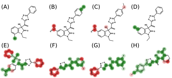
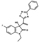
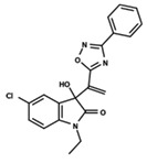
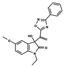
In addition to the predictive capacity, KPLS 2D-QSAR allows the visualization of regions in the molecules responsible for increasing or decreasing the biological response through the generation of contribution maps, as depicted in Figure 4. Green and red colors represent positive and negative contributions to response, respectively. For the G₁ group, halogen substituents showed positive contributions to substituents R₁, R₃, R₄ and R₅. The only difference among molecules 7, 22, and 23 is the substitution of bromine, fluorine, and chlorine in substituent R₃, and all substitutions in this position showed positive contributions. However, the chlorine in molecule 23 contributed to a greater increase in activity, which can be validated directly by the pIC₅₀ in Table 4. In general, the nitro group substitution was unfavorable for molecules in G₁. For the G₂ group, the hydrogen atom in position R₁ showed an unfavorable contribution. In this case, the phenyl group, and especially the methoxy group substitution, showed a favorable contribution in R₁. An exception for the positive contribution of the nitro group was observed with the oxazole core. In substituent R₃, halogen (except bromide) and nitro substituents showed a positive contribution, but asymmetrical electron density was slightly unfavorable, which favors double halogen substitutions in both meta positions or one halogen in the para position. For substituent R₂, the hydroxyl group showed a positive contribution, while the benzene sulfonamide showed a negative contribution.

Figure 4.

Contribution map generated by KPLS of groups G₁ (A–D) and G₂ (E–H). Green colors represent positive contributions, and red colors indicate negative contributions to biological activity.

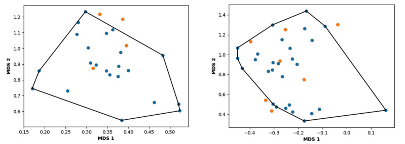
The MDS scatter plot of the dataset, obtained by the geometric convex-hull method, allows the definition of the chemical space over which the model, represented by the training set, is applicable. The applicability domain for the 2D-QSAR models for the G₁ and G₂ groups is shown in Figure 5.

Figure 5.

Applicability domain for group G₁ (left) and group G₂ (right). The molecules of the training set are illustrated in blue, and the compounds of the test set are depicted in orange.

2.2. 4D-QSAR

Three-dimensional quantitative structure–activity relationship (3D-QSAR) modeling is a broadly used method in computer-assisted molecular design. The method assumes that changes in the binding affinities of ligands are related to changes in molecular properties represented by molecular fields. A common and popular method is comparative molecular field analysis (CoMFA). Some issues are inherent in 3D-QSAR [15,16], mainly in receptor-independent 3D-QSAR (RI-3D-QSAR). For example, the QSAR model in the CoMFA method is strongly dependent and sensitive to conformations and alignments of the molecules. Another limitation is that the bioactive conformation of a molecule should be used, which may not coincide with the lowest energy conformations, which are commonly used whenever the molecular target is unknown. In this work, several structural alignment methods were used as attempts to achieve a suitable alignment of the compounds to be used in subsequent CoMFA analyses. However, due to the limitations described above, no suitable CoMFA models were obtained (see Supplementary File for CoMFA models). Following these concepts, a 4D-QSAR approach was used in this work to address the limitations associated with 3D-QSAR models. The LQTA-QSAR approach explores the main advantages of both CoMFA and 4D-QSAR modeling [16,17]. This method is based on the generation of a CEP for each compound instead of only one conformation, which is followed by the calculation of 3D descriptors using the Coulomb and Lennard–Jones potentials. To generate the 4D-QSAR models, the strategy used in the 2D-QSAR analyses was repeated, i.e., we built a model with the entire dataset, which was followed by the generation of groups by using hierarchical clustering. Two-hundred training and test sets were randomly divided and subjected to QSAR model construction. For the 2D-QSAR studies, the best results were obtained by using an 80:20 ratio between the training and test sets; thus, the same ratio was applied to the 4D-QSAR analyses.

The model generated using the complete dataset was used for comparison purposes. LQTAgridPy software was used to generate a matrix with 21,252 descriptors. After applying a variance cutoff and the Pearson cutoff, 554 descriptors were subjected to PyQSAR. This software uses a clustering method to reduce the search space. In this step, PyQSAR also eliminates descriptors with low variance. A selection based on a genetic algorithm (GA) was used to maintain the best descriptors from the different clusters. The GA-based selections were repeated until the optimal variable selection was achieved. PyQSAR selected a set of descriptors that resulted in the following parameters: R² = 0.4599, R²_{pred =} 0.4353. The set of selected descriptors included [15_19_20_NH3+_C], [15_20_15_NH3+_LJ], [16_21_20_NH3+_C], [16_23_10_NH3+_LJ], and [18_19_11_NH3+_C].

Group G₁: The dataset used in the 4D-QSAR for G₁ was the same as that previously used in the 2D-QSAR, with 27 compounds divided into 22 molecules for the training set and 5 compounds for the test set. The LQTAgridPy software resulted in a matrix with 19,404 descriptors. After truncation of the Lennard–Jones potential, the variance cutoff, and the Pearson cutoff, the filters led to a significant variable reduction to 903 descriptors. Each of these descriptors represents a grid point with the fields acting upon it. This reduced matrix was used as the input for the selection of variables and generation of the model by PyQSAR. The model chosen is represented by 5 descriptors (Equation (1)) and generated the following results: R² = 0.8033, RMSE = 0.1313, Q²_{5-fold =} 0.6600, RMSE_{cv =} 0.1716, R²_{pred =} 0.6480.

pIC₅₀ = 5.1535 + 0.8409[15_13_6_NH3+_LJ]
−0.7075[16_12_5_NH3+_LJ]
+0.1484[16_20_10_NH3+_LJ]
−0.1210[21_17_13_NH3+_LJ]
+0.1913[22_12_12_NH3+_LJ] (1)

Group G₂: For G₂, the same 35 compounds used in 2D-QSAR, divided into 28 compounds in the training set and 7 in the test set, were employed in the 4D-QSAR. The LQTAgridPy software resulted in a matrix with 21,252 descriptors. After truncation of the Lennard–Jones potential, the variance cutoff, and the Pearson cutoff, the filters led to a significant variable reduction to 3353 descriptors. Each of these descriptors represents a grid point with the fields acting on it. This reduced matrix was used as the input for the selection of variables and generation of the model by PyQSAR. The selected model is represented by five descriptors (Equation (2)) and generated the following results: R² = 0.7005, RMSE = 0.156, Q²_{5-fold =} 0.6095, RMSE_{cv =} 0.1701, R²_{pred =} 0.6581.

pIC₅₀ = 4.9338 + 0.2170[16_20_11_NH3+_LJ]
+0.1303[17_19_15_NH3+_LJ]
−0.7328[17_26_15_NH3+_C]
+0.2770[18_23_14_NH3+_LJ]
+0.7227[19_26_20_NH3+_C] (2)

The 4D-QSAR statistical parameters are summarized in Table 5.

Table 5.

Statistically significant 4D-QSAR models.

Dataset	R 2	RMSE	Q 2 5-fold	RMSEcv	R 2 pred
Complete dataset	0.4599	0.2277	0.4137	0.2412	0.4353
G1	0.8033	0.1313	0.6600	0.1716	0.6480
G2	0.7005	0.1560	0.6095	0.1701	0.6581

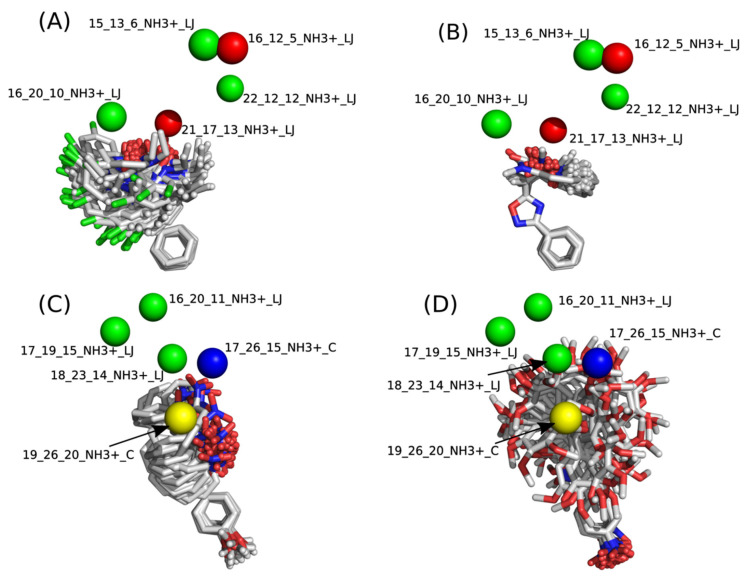
The contribution maps were generated to allow the visualization of the positive and negative contributions of groups in the 4D-QSAR model (Figure 6). Green spheres represent steric interactions with positive regression coefficients, and red represents steric interactions with negative regression coefficients. Similarly, blue spheres indicate electrostatic descriptors with negative regression coefficients, and yellow represents positive regression coefficients. Positive coefficients contribute positively to the pIC₅₀ values, while negative coefficients contribute negatively. The analysis for both groups G₁ and G₂ indicates that the major correlation between structure and activity is not related to the oxadiazole or oxazole core, but primarily to the substituents attached to these rings.

Figure 6.

Contribution maps of the most and least potent compounds of group G₁ (A,B) and group G₂ (C,D).

Group G₁: For G₁, the positive steric contributions [16_20_10_NH3+_LJ] and [22_12_12_NH3+_LJ] are mainly related to the halogen substituents at R₄ and R₅, which, due to energy minimization, are facing towards [16_20_10_NH3+_LJ] or [22_12_12_NH3+_LJ] in some of these molecules. The negative steric contribution [21_17_13_NH3+_LJ] is related to the hydroxyl group, and mainly to bulky substituents at R₂. The results of the 4D-QSAR models for G₁ are related to the degree of flexibility and pIC₅₀. Molecules with a higher degree of freedom showed poor biological activity, which may pose an obstacle to the formation of stable intermolecular interactions with the molecular target [18].

Group G₂: For G₁, a higher conformational degree of freedom of the molecules is also associated with low pIC₅₀ values, which can be noticed in Figure 6 when comparing the least and most active compounds. The descriptor [18_23_14_NH3+_LJ] indicates that bulky substituents at group R₃, mainly represented by compound 31 with an ethenylbenzene (styrene) substituent, show a positive steric contribution. The positive contribution of [19_26_20_NH3+_C] is associated with halogen-substituted compounds in the para position of the phenyl in group R₄, whereas the [17_26_15_NH3+_C] contribution indicates that these same atoms can decrease the biological response because of the assumed conformations.

3. Materials and Methods

3.1. Dataset Characterization

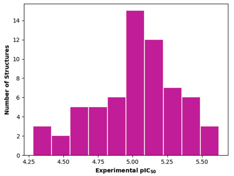
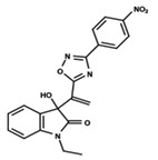
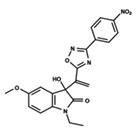
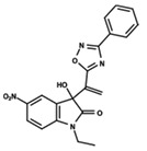
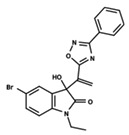
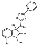
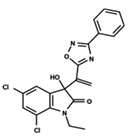
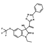
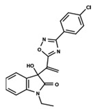
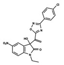
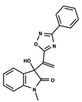
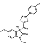
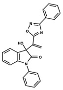
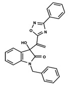
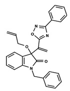
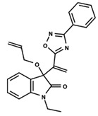
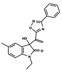
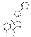
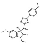
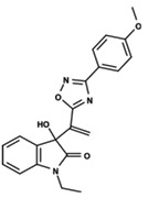
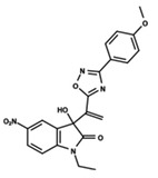
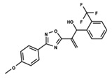
The dataset used for both QSAR modeling methods includes 64 molecules, 62 having an oxadiazole ring and 2 having an oxazole core, as shown in Table 6. The in vitro assays against L. infantum were performed in our research group using the same experimental conditions, as previously reported [4]. The potency of the compounds was expressed as the concentration required to kill 50% of parasites in vitro (IC₅₀). The antileishmanial activity was determined as the number of intracellular amastigotes in THP-1 macrophages, which is the relevant form of the parasite for drug discovery purposes. The IC₅₀ values (ranging from 2.38 to 52.59 µM) were converted into pIC₅₀ values for appropriately scaling the data, which ranged from 4.28 to 5.62. The distribution of pIC₅₀ values over the dataset compounds is illustrated in the histogram in Figure 7.

Table 6.

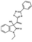
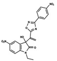
Structures and pIC₅₀ values of the dataset compounds used in the QSAR studies.

No.	Structure	pIC50 exp	No.	Structure	pIC50 exp	No.	Structure	pIC50 exp
1		5.138	2		4.913	3		5.133
4		5.478	5		4.922	6		5.29
7		5.428	8		4.984	9		5.387
10		4.955	11		5.397	12		5.188
13		4.289	14		5.293	15		5.088
16		5.248	17		4.97	18		4.931
19		5.313	20		5.193	21		5.221
22		5.455	23		5.602	24		5.314
25		5.137	26		4.658	27		5.545
28		4.587	29		5.033	30		5.115
31		5.084	32		4.592	33		5.081
34		4.976	35		5.096	36		4.932
37		5.135	38		4.981	39		4.598
40		4.279	41		4.426	42		5.11
43		4.755	44		4.723	45		4.358
46		4.985	47		4.988	48		4.663
49		4.744	50		4.92	51		5.049
52		4.687	53		4.445	54		5.41
55		5.068	56		4.94	57		5.623
58		5.008	59		5.072	60		5.137
61		5.291	62		5.07	63		4.747
64		5.16

Figure 7.

Histogram for the distribution of the experimental pIC₅₀ values over the entire compound set used in the QSAR studies.

In addition to the characterization of the activity profile of the dataset, a scaffold analysis was performed for the R-groups using Canvas (Maestro, Schrödinger) [19]. The general scaffolds for the series were generated through an automated search for the maximum common substructure (MCS).

3.2. 2D-QSAR

The 2D-QSAR was performed with the machine learning tools of AutoQSAR [19] embedded in Maestro [20] (release 2016-3, Schrödinger LLC, New York, NY, USA) as previously reported [21,22]. In all AutoQSAR calculations, the proportion between the test and training sets was defined as follows: 70:30 (70% of the compounds for training the models and 30% for the test set), 75:25, and 80:20. The best model was selected based on internal validation parameters, such as the regression coefficient (R²) and the 8 standard deviation (SD) for the training set, and external validation parameters, i.e., the predicted regression coefficient (Q²) and the root-mean-square error (RMSE) for the test set compounds. The best models were recreated within Canvas using the same test set, training set, and binary fingerprint generated in the AutoQSAR modeling.

3.3. Hierarchical Clustering

Hierarchical clustering based on 2D similarity analyses of the dataset was performed using Canvas 1.1 software. Linear fingerprints were calculated, and the similarity matrix was evaluated using the Tanimoto coefficient as the similarity metric [23]. This is a popular similarity metric for comparing chemical structures represented by means of fingerprints, and structures are usually considered similar if the index is higher than 0.85. A higher number of shared features results in an index closer to 1. Conversely, a higher number of unique features results in an index closer to zero. The agglomerative method chosen was the average linkage. Based on the similarity results, the dataset compounds were split into two groups, and the Kelley index was used to select the optimal number of clusters [12]. Following this procedure, the number of clusters was decreased to generate two different groups so that if the number of clusters was reduced again, it would result in the merging of groups G₁ and G₂. To visualize the diversity of the identified groups in a plane, a multidimensional scaling (MDS) approach was employed with the similarity matrix as input in a Knime node [24].

The applicability domain (AD) defines a region or limits where the model is able to reliably perform according to predictions [25]. The AD generated in this work was built using the geometric convex-hull method [26]. After the MDS, the coordinates of the training set were submitted to SciPy to generate the convex-hull output.

3.4. 4D-QSAR

The 4D-QSAR was performed with the LQTA-QSAR method [27]. The molecular dynamics simulation was performed using GROMACS version 4.6.5 [28,29]. A dodecahedron box was filled with explicit transferable intermolecular potential 3-point (TIP3P) water molecules, and the ffG43a1 [30,31] force field was used for the all-atom molecular simulations. The minimum distance between the molecule and walls was set to 10 Å. The energy minimization step was performed using the steepest descent gradient and conjugate gradient methods for a maximum of 4000 calculation steps. The pressure of the system was controlled by Parrinello–Rahman [32] coupling, and the temperature was kept constant by the Berendsen thermostat [33]. The volume of the system was balanced by heating in steps of 50 K, 100 K, 200 K, and 350 K for 10 ps each, and the system was ultimately cooled to 300 K for a 500 ps simulation. All the conformations for each ligand obtained through molecular dynamics simulations were placed in a “.gro” file extension. The conformational ensemble profile (CEP) to be used for the 4D-QSAR models was assembled considering the ligand conformations obtained from 50 to 500 ps. The alignment was generated considering the matching of the atom positions of the oxazole and oxadiazole rings. The alignment was submitted to LQTAgridPy, a Python version of LQTAgrid. The probe NH⁺³ was selected and used to represent the N-terminal unit. The probe swept all grid points from the box to compute all Coulomb and Lennard–Jones descriptors. The data were preprocessed with the energy cutoff of the Lennard–Jones descriptors from the CoMFA method. If the descriptor computed at an x, y, z position had a value of Lennard–Jones energy equal to or lower than 30 kcal/mol, no cutoff was applied. Otherwise, if the energy value exceeded 30 kcal/mol, then the logarithmic value of the residual was added to 30 kcal/mol, according to the following:

LJ_x,y,z < 30 kcal/mol → LJ_x,y,z = LJ_x,y,z
LJ_x,y,z ≥ 30 kcal/mol → L J_x,y,z = 30 + logLJ_x,y,z − 30

The filtering method for the descriptor selection excluded those variables with absolute values of the Pearson correlation coefficient (|r|) of less than 0.2 with respect to the pIC₅₀ [18,27] and the low-variance descriptors that only slightly changed between compounds (those with variance below the cutoff value of 0.01). The remaining descriptors were selected by PyQSAR [34], an open-source QSAR model generator. The variable selection used in PyQSAR uses the strategies of hierarchical clustering and a genetic algorithm (GA). Finally, multiple linear regression (MLR) was performed with the generated descriptors, and the pIC₅₀ values were used as the independent variables to build the model. The process of internal validation was carried out through conventional noncross-validated correlation (R²). The robustness was examined by 5-fold cross-validated correlation (Q²_5-fold) coefficients. For external validation, the test set was evaluated according to the coefficient of determination of external validation (R²_pred). The images of the contribution maps were created by using PyMOL version 1.8.4.0 [35].

4. Conclusions

Receptor-independent QSAR methods were employed in the development of 2D- and 4D-QSAR models for a series of oxadiazole and oxazole antileishmanial derivatives. The clustering of the dataset proved to be advantageous for optimizing the statistical parameters in both the 2D-QSAR and 4D-QSAR models presented in this work. The final models exhibited good internal consistency and external predictive power and were able to accurately predict the pIC₅₀ values when compared to the experimental values for both 2D and 4D models within the applicability domain. Once new compounds are designed, the hierarchical clustering, MDS plot, and applicability domain are useful tools to evaluate which group they belong to, and then the corresponding model can be applied. The results for the 2D-QSAR models compared to that of the 4D models suggest that for this dataset, 2D descriptors correlate better to the variation in the biological activity. The reasons for poorer results in QSAR methods that require 3D conformations are unknown; however, they may be linked to the mode of action of this series, which is yet to be discovered. Although the molecular target of these compounds is so far unknown, we can speculate from the structure of the compounds that the several functionalities that are able to form hydrogen-bonds and π-stacking interactions play a significant role in the biological activity of this series, for example, the hydroxy-oxyindole, phenyl and oxadiazole rings. However, the exact role of each functionality in terms of ligand–target complexes could only be disclosed after the discovery and structural resolution of the molecular target. In addition to the activity prediction, the generated 2D and 4D contribution maps provided information about structural and conformational features that can be used as a valuable tool to guide future efforts in the design of antileishmanial agents.

Supplementary Materials

The following supporting information can be downloaded at: https://www.mdpi.com/article/10.3390/ijms23168898/s1.

Author Contributions

Conceptualization, H.R.T., L.L.G.F., M.V., F.C. and A.D.A.; Formal analysis, H.R.T., L.L.G.F. and M.V.; Funding acquisition, A.D.A.; Investigation, H.R.T., L.L.G.F., M.V., F.C. and A.D.A.; Supervision, A.D.A.; Writing—original draft, H.R.T., L.L.G.F. and M.V.; Writing—review & editing, H.R.T., L.L.G.F., M.V., F.C. and A.D.A. All authors have read and agreed to the published version of the manuscript.

Institutional Review Board Statement

Not applicable.

Informed Consent Statement

Not applicable.

Data Availability Statement

Not applicable.

Conflicts of Interest

The authors declare they have no conflict of interest.

Funding Statement

The authors acknowledge the National Council for Scientific and Technological Development (CNPq), the Coordination for the Improvement of Higher Education Personnel (CAPES), and the Sao Paulo Research Foundation (FAPESP) (CIBFar grant 2013/07600-3; M.V. grant 2019/05967-3), Brazil, for financial support.

References

- 1.Ruiz-Postigo J.A., Grout L., Saurabh J. Global leishmaniasis surveillance, 2017–2018, and first report on 5 additional indi cators/Surveillance mondiale de la leishmaniose, 2017–2018, et premier rapport sur 5 indicateurs supplementaires. Wkly. Epidemiol. Rec. 2020;95:265–280. [Google Scholar]
- 2.Polonio T., Efferth T. Leishmaniasis: Drug resistance and natural products. Int. J. Mol. Med. 2008;22:277–286. doi: 10.3892/ijmm_00000020. [DOI] [PubMed] [Google Scholar]
- 3.Gourbal B., Sonuc N., Bhattacharjee H., Legare D., Sundar S., Ouellette M., Rosen B.P., Mukhopadhyay R. Drug uptake and modulation of drug resistance in Leishmania by an aquaglyceroporin. J. Biol. Chem. 2004;279:31010–31017. doi: 10.1074/jbc.M403959200. [DOI] [PubMed] [Google Scholar]
- 4.Fernandes F.S., Santos H., Lima S.R., Conti C., Rodrigues M.T., Jr., Zeoly L.A., Ferreira L.L., Krogh R., Andricopulo A.D., Coelho F. Discovery of highly potent and selective antiparasitic new oxadiazole and hydroxy-oxindole small molecule hybrids. Eur. J. Med. Chem. 2020;201:112418. doi: 10.1016/j.ejmech.2020.112418. [DOI] [PubMed] [Google Scholar]
- 5.Gilbert I.H. Drug discovery for neglected diseases: Molecular target-based and phenotypic approaches: Miniperspectives series on phenotypic screening for antiinfective targets. J. Med. Chem. 2013;56:7719–7726. doi: 10.1021/jm400362b. [DOI] [PMC free article] [PubMed] [Google Scholar]
- 6.Ferreira L.L., de Moraes J., Andricopulo A.D. Approaches to advance drug discovery for neglected tropical diseases. Drug Discov. Today. 2022;27:2278–2287. doi: 10.1016/j.drudis.2022.04.004. [DOI] [PubMed] [Google Scholar]
- 7.Taha M., Ismail N.H., Ali M., Rashid U., Imran S., Uddin N., Khan K.M. Molecular hybridization conceded exceptionally potent quinolinyl-oxadiazole hybrids through phenyl linked thiosemicarbazide antileishmanial scaffolds: In silico validation and SAR studies. Bioorganic Chem. 2017;71:192–200. doi: 10.1016/j.bioorg.2017.02.005. [DOI] [PubMed] [Google Scholar]
- 8.Taha M., Ismail N.H., Imran S., Selvaraj M., Jamil W., Ali M., Kashif S.M., Rahim F., Khan K.M., Adenan M.I., et al. Synthesis and molecular modelling studies of phenyl linked oxadiazole-phenylhydrazone hybrids as potent antileishmanial agents. Eur. J. Med. Chem. 2017;126:1021–1033. doi: 10.1016/j.ejmech.2016.12.019. [DOI] [PubMed] [Google Scholar]
- 9.Pitasse-Santos P., Sueth-Santiago V., Lima M.E. 1,2,4-and 1,3,4-Oxadiazoles as Scaffolds in the Development of Antiparasitic Agents. J. Braz. Chem. Soc. 2018;29:435–456. doi: 10.21577/0103-5053.20170208. [DOI] [Google Scholar]
- 10.Scala A., Cordaro M., Grassi G., Piperno A., Barberi G., Cascio A., Risitano F. Direct synthesis of C3-mono-functionalized oxindoles from N-unprotected 2-oxindole and their antileishmanial activity. Bioorganic Med. Chem. 2014;22:1063–1069. doi: 10.1016/j.bmc.2013.12.039. [DOI] [PubMed] [Google Scholar]
- 11.Saha S., Acharya C., Pal U., Chowdhury S.R., Sarkar K., Maiti N.C., Jaisankar P., Majumder H.K. A novel spirooxindole derivative inhibits the growth of Leishmania donovani parasites both in vitro and in vivo by targeting type IB topoisomerase. Antimicrob. Agents Chemother. 2016;60:6281–6293. doi: 10.1128/AAC.00352-16. [DOI] [PMC free article] [PubMed] [Google Scholar]
- 12.Kelley L.A., Gardner S.P., Sutcliffe M.J. An automated approach for clustering an ensemble of NMR-derived protein structures into conformationally related subfamilies. Protein Eng. Des. Sel. 1996;9:1063–1065. doi: 10.1093/protein/9.11.1063. [DOI] [PubMed] [Google Scholar]
- 13.Santos-Filho O.A., Cherkasov A. Using molecular docking, 3D-QSAR, and cluster analysis for screening structurally diverse data sets of pharmacological interest. J. Chem. Inf. Model. 2008;48:2054–2065. doi: 10.1021/ci8001952. [DOI] [PubMed] [Google Scholar]
- 14.Tropsha A. Best Practices for QSAR Model Development, Validation, and Exploitation. Mol. Inform. 2010;29:476–488. doi: 10.1002/minf.201000061. [DOI] [PubMed] [Google Scholar]
- 15.Hopfinger A., Wang S., Tokarski J.S., Jin B., Albuquerque M., Madhav P.J., Duraiswami C. Construction of 3D-QSAR models using the 4D-QSAR analysis formalism. J. Am. Chem. Soc. 1997;119:10509–10524. doi: 10.1021/ja9718937. [DOI] [Google Scholar]
- 16.Ghasemi J.B., Safavi-Sohi R., Barbosa E.G. 4D-LQTA-QSAR and docking study on potent gram-negative specific LpxC inhibitors: A comparison to CoMFA modeling. Mol. Divers. 2012;16:203–213. doi: 10.1007/s11030-011-9340-3. [DOI] [PubMed] [Google Scholar]
- 17.Cramer R.D., Patterson D.E., Bunce J.D. Comparative molecular field analysis (CoMFA). 1. Effect of shape on binding of steroids to carrier proteins. J. Am. Chem. Soc. 1988;110:5959–5967. doi: 10.1021/ja00226a005. [DOI] [PubMed] [Google Scholar]
- 18.Melo E., Ferreira M. A 4D structure-activity relationship model to predict HIV-1 integrase strand transfer inhibition using the LQTA-QSAR methodology. J. Chem. Inf. Model. 2012;52:1722–1732. doi: 10.1021/ci300039a. [DOI] [PubMed] [Google Scholar]
- 19.Dixon S.L., Duan J., Smith E., von Bargen C.D., Sherman W., Repasky M.P. AutoQSAR: An automated machine learning tool for best-practice quantitative structure–activity relationship modeling. Future Med. Chem. 2016;8:1825–1839. doi: 10.4155/fmc-2016-0093. [DOI] [PubMed] [Google Scholar]
- 20.Release S. Maestro. Schrödinger LLC; New York, NY, USA: 2017. Version 3. [Google Scholar]
- 21.Medeiros A.R., Ferreira L.L., de Souza M.L., de Oliveira Rezende C., Jr., Espinoza-Chávez R.M., Dias L.C., Andricopulo A.D. Chemoinformatics Studies on a Series of Imidazoles as Cruzain Inhibitors. Biomolecules. 2021;11:579. doi: 10.3390/biom11040579. [DOI] [PMC free article] [PubMed] [Google Scholar]
- 22.De Souza A.S., Ferreira L.L., de Oliveira A.S., Andricopulo A.D. Quantitative Structure-Activity Relationships for Structurally Diverse Chemotypes Having Anti-Trypanosoma cruzi Activity. Int. J. Mol. Sci. 2019;20:2801. doi: 10.3390/ijms20112801. [DOI] [PMC free article] [PubMed] [Google Scholar]
- 23.Maggiora G., Vogt M., Stumpfe D., Bajorath J. Molecular similarity in medicinal chemistry: Miniperspective. J. Med. Chem. 2014;57:3186–3204. doi: 10.1021/jm401411z. [DOI] [PubMed] [Google Scholar]
- 24.Berthold M.R., Cebron N., Dill F., Gabriel T.R., Kötter T., Meinl T., Ohl P., Thiel K., Wiswedel B. KNIME—The Konstanz Information Miner: Version 2.0 and Beyond. SIGKDD Explor. Newsl. 2009;11:26–31. doi: 10.1145/1656274.1656280. [DOI] [Google Scholar]
- 25.Weaver S., Gleeson M.P. The importance of the domain of applicability in QSAR modeling. J. Mol. Graph. Model. 2008;26:1315–1326. doi: 10.1016/j.jmgm.2008.01.002. [DOI] [PubMed] [Google Scholar]
- 26.Sahigara F., Mansouri K., Ballabio D., Mauri A., Consonni V., Todeschini R. Comparison of different approaches to define the applicability domain of QSAR models. Molecules. 2012;17:4791–4810. doi: 10.3390/molecules17054791. [DOI] [PMC free article] [PubMed] [Google Scholar]
- 27.Martins J.P.A., Barbosa E.G., Pasqualoto K.F., Ferreira M.M. LQTA-QSAR: A new 4D-QSAR methodology. J. Chem. Inf. Modeling. 2009;49:1428–1436. doi: 10.1021/ci900014f. [DOI] [PubMed] [Google Scholar]
- 28.Bekker H., Berendsen H., Dijkstra E., Achterop S., Vondrumen R., Vanderspoel D., Sijbers A., Keegstra H., Renardus M. Physics Computing ’92. World Scientific Publishing; Singapore: 1993. Gromacs-a parallel computer for molecular-dynamics simulations; pp. 252–256. [Google Scholar]
- 29.Berendsen H.J., van der Spoel D., van Drunen R. GROMACS: A message-passing parallel molecular dynamics implementation. Comput. Phys. Commun. 1995;91:43–56. doi: 10.1016/0010-4655(95)00042-E. [DOI] [Google Scholar]
- 30.Schuler L.D., Daura X., van Gunsteren W.F. An improved GROMOS96 force field for aliphatic hydrocarbons in the condensed phase. J. Comput. Chem. 2001;22:1205–1218. doi: 10.1002/jcc.1078. [DOI] [Google Scholar]
- 31.Chandrasekhar I., Kastenholz M., Lins R.D., Oostenbrink C., Schuler L.D., Tieleman D.P., van Gunsteren W.F. A consistent potential energy parameter set for lipids: Dipalmitoylphosphatidylcholine as a benchmark of the GROMOS96 45A3 force field. Eur. Biophys. J. 2003;32:67–77. doi: 10.1007/s00249-002-0269-4. [DOI] [PubMed] [Google Scholar]
- 32.Parrinello M., Rahman A. Crystal Structure and Pair Potentials: A Molecular-Dynamics Study. Phys. Rev. Lett. 1980;45:1196–1199. doi: 10.1103/PhysRevLett.45.1196. [DOI] [Google Scholar]
- 33.Berendsen H.J., Postma J.V., van Gunsteren W.F., DiNola A., Haak J.R. Molecular dynamics with coupling to an external bath. J. Chem. Phys. 1984;81:3684–3690. doi: 10.1063/1.448118. [DOI] [Google Scholar]
- 34.Kim S., Cho K.H. PyQSAR: A fast QSAR modeling platform using machine learning and Jupyter notebook. Bull. Korean Chem. Soc. 2019;40:39–44. doi: 10.1002/bkcs.11638. [DOI] [Google Scholar]
- 35.Schrödinger, LLC . The PyMOL Molecular Graphics System. Schrödinger Inc.; New York, NY, USA: 2016. Version 1.8. [Google Scholar]
Associated Data
This section collects any data citations, data availability statements, or supplementary materials included in this article.