Machine learning-driven new material discovery

Abstract

New materials can bring about tremendous progress in technology and applications. However, the commonly used trial-and-error method cannot meet the current need for new materials. Now, a newly proposed idea of using machine learning to explore new materials is becoming popular. In this paper, we review this research paradigm of applying machine learning in material discovery, including data preprocessing, feature engineering, machine learning algorithms and cross-validation procedures. Furthermore, we propose to assist traditional DFT calculations with machine learning for material discovery. Many experiments and literature reports have shown the great effects and prospects of this idea. It is currently showing its potential and advantages in property prediction, material discovery, inverse design, corrosion detection and many other aspects of life.

This paper summarizes the ideas, operations and workflows of how machine learning has driven the discovery of new materials.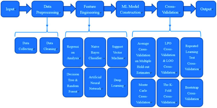

1. Introduction

Machine learning (ML)^1,2 is a new subfield of artificial intelligence that focuses on optimizing computer programs to improve algorithms through data and researching experience. ML has also become an efficient and important tool for analysing existing materials in the field of new material discovery.^3,4 The traditional trial-and-error method relies on personal experience. Therefore, decades often pass from experiment to marketing.^5,6 Considering the consumption of experimental development, the traditional material discovery method can hardly adapt to the large-scale demand for novel high-performance materials.

To address this situation, the United States of America launched the “Material Genome Initiative” project (MGI) in 2011.⁷ The MGI proposes that researchers should focus on “material design” instead of “trial-and-error”, which requires researchers to deepen their comprehension of materials; collect enormous material data to build databases and computing platforms; and above all, use high-throughput screening of materials to eventually achieve the purpose of reducing research costs and speeding development. In 2016, China launched the “Material Genetic Engineering and Support Platform” program as a national strategy. Different from MGI, the Chinese government is concerned with building a high-throughput computing platform⁸ that can serve the majority of researchers. In this aspect, machine learning-driven new material discovery is thriving.

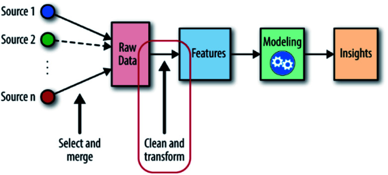
When solving material problems by ML, datasets are needed to help detect target features, properties or unknown materials. These datasets and the messages inside them are called “input”, and the targets are called “output”. With these two definitions, the ML-aided method can now be defined as “using inputs and appropriate ML algorithms to build a numerical predicting model and detecting unknown outputs by the predicting ability of this model” (Fig. 1). Because outputs are fitted by inputs, it is reasonable that the outputs will have similar chemical structures to the inputs and can be evaluated in the same way that the inputs are evaluated.⁹ With this model, we can enhance the comprehension of material properties and predict unknown needed materials. At present, this method is still confronted with many challenges: the messy datasets must be preprocessed; the accuracy of the model is limited by its algorithms; the high-intensity computation places pressure on computing resources; etc.¹⁰

Fig. 1. The machine learning workflow; the place of feature engineering is shown in the red circle.¹¹.

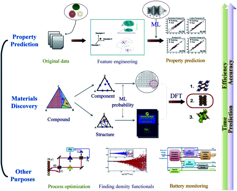
Machine learning has been widely used in many aspects of material science (Fig. 2). In this review, we focus on model construction, computational algorithms, model verification procedures, the role ML plays in the material science field and the prospects of machine learning. Section 2 describes the data preprocessing and feature engineering steps, which can systemically reconstruct the datasets and aid understanding of material properties and physicochemical relationships. In Section 3, some high-performance algorithms in the material discovery field are introduced, and some practical application examples in this field are surveyed. Section 4 describes several cross-validation procedures for material-discovery ML models. Section 5 explains how ML assists traditional density functional theory in the field of materials science. In Section 6, some other artificial intelligence methods that ML is involved in are discussed. In Section 7, we will summarize the current development condition of ML methods and briefly explain the prospects of ML in new material discovery.

Fig. 2. An overview of the application of machine learning in materials science.¹².

2. Data preprocessing and feature engineering

Data is very important in ML procedures. Generally, the final ML results can be directly affected by the volume and reliability of data; this is where data preprocessing and feature engineering come in. These two steps can reconstruct datasets so that it is more convenient for computers to understand material physicochemical relationships, detect material properties and establish material predicting models.^13–15 For example, Paul Raccuglia once proposed that a predicting model can be trained by data from failed experiments. He integrated experimental data using information from failed or less successful hydrothermal synthesis reactions to train a machine learning model to predict the crystallization of template vanadium selenite crystals. It was found that this model was obviously superior compared with the traditional manual analysis method. The prediction accuracy for the formation conditions of new organic-templated inorganic products could reach 89%.⁵

In the following parts, we will introduce the two main steps of data preprocessing and how they function in material discovery; we will also give some examples of successful applications in the material field.

2.1. Data preprocessing

Data preprocessing mainly consists of two steps: data collecting and data cleaning.¹⁶

i. Data collecting

Researchers always hope to collect representative data. Therefore, it is necessary for researchers to select the appropriate data for specific problems. Currently, numerous open-source databases, such as the Harvard Clean Energy Project, the Open Quantum Materials Database and the Materials Project,¹⁷ have been established. These databases are reliable and accessible and can be used as a bedrock of research work. Some of the most authoritative and reliable databases are listed below for reference (Table 1).

An overview of some of the most authoritative databases in material science.

Title	Website address	Brief introduction
AFLOWLIB	http://www.aflowlib.org	A global database of 3 249 264 material compounds and over 588 116 784 calculated properties
ASM Alloy Database	https://www.asminternational.org/materials-resources/online-databases	An authoritative database focusing on alloys, mechanical and alloy phases, and failed experiment data
Cambridge Crystallographic Data Centre	http://www.ccdc.cam.ac.uk	It focuses on structural chemistry and contains over 1 000 000 structures
ChemSpider	http://www.chemspider.com	A free chemical structural database providing fast searching access to over 67 000 000 structures
Harvard Clean Energy Project	http://cepdb.molecularspace.org/	A massive database of organic solar cell materials
High Performance Alloys Database	https://cindasdata.com/products/hpad	This high performance alloy database addresses the needs of the chemical processing, power generation and transportation industries
Materials Project	https://materialsproject.org/	It offers more than 530 000 nanoporous materials, 124 000 inorganic compounds and power analysis tools for researchers
NanoHUB	https://nanohub.org/resources/databases	An open source database focusing on nanomaterials
Open Quantum Materials Database	http://oqmd.org/	It contains substantial amounts of data on the thermodynamic and structural properties of 637 644 materials
Springer Materials	http://materials.springer.com	A comprehensive database covering multiple material classes, properties and applications

For example, Edward O. Pyzer-Knapp's team used the data from the Harvard Clean Energy Database for ML model training to solve the over-provisioning problem, in which computers mistakenly consider noise to be useful features. According to the results, the trained ML model can return predictions on the verification set within 1.5 seconds, and the over-provisioning problem is successfully solved.¹⁸ Kamal Choudhary's team established a criterion to identify 2D materials based on comparison of lattice constants obtained from experiments and the Materials Project Database. Also, to test this criterion, they calculated the exfoliation of many layered materials. The results showed that in 88.9% of cases, the criterion was satisfied.¹⁹ T. Björkman's team screened the International Crystallographic Structural Database (ICSD) and discovered 92 possible 2D compounds based on symmetry, packing ratio, structural gaps and covalent radii.²⁰ In other cases, Michael Ashton and colleagues used the topology-scaling algorithm to detect layered materials from ICSD and successfully found 680 stable monolayers;²¹ Nicolas Mounet and coworkers used data mining of ICSD and the Crystallographic Open Database to search for layered compounds;²² and Sten Haastrup's team established one of the largest databases of 2D materials.²³ All the research mentioned above strongly supports the availability and superiority of high-quality data in practical applications. From this point of view, this is a necessary step of the ML method in material discovery.

ii. Data cleaning

After the data collection step, there are still many problems with the collected data, such as data redundancy or abnormal values. In order to obtain an efficient ML predicting model and also to reduce the amount of calculation, data cleaning is necessary. In this paper, we define data cleaning as a data operation consisting of four steps: data sampling, abnormal value processing, data discretization, and data normalization.^24,25

First, data sampling ensures that researchers can obtain high performance prediction models with less data without compromising predicting accuracy.²⁶ To ensure the ability and accuracy of the predicting model, researchers must eliminate abnormal values to maintain the accuracy of the predicting models.²⁷ Furthermore, data discretization can significantly reduce the number of possible values of a continuous feature. Also, data normalization can adjust the magnitudes of data to a suitable and identical level, which is crucial for many machine learning algorithms. As an example, in the research of photovoltaic organic-inorganic hybrid perovskites by Shuai Hua Lu's team, all the input data were obtained from reliable databases composed of high throughput first-principles calculations. For data consistency and accuracy of the ML predictions, they carefully constructed their own training sets and validation sets with appropriately processed data. Only orthorhombic-like crystal structures with bandgaps calculated using the Perdew–Burke–Ernzerhof (PBE) functional were selected.²⁸

Also, after the four steps above, the dataset is divided into training sets and testing sets. As we can see, after data preprocessing, the noise, data redundancy and abnormal values are all largely reduced. However, the dataset is still messy. It must be reconstructed to enable computers to better understand the data within. This can be achieved by feature engineering.

2.2. Feature engineering

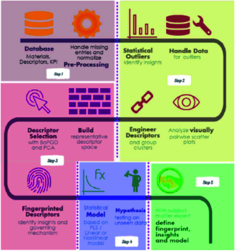
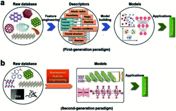
Feature engineering is the process of extracting the most appropriate features from data and tasks. These features are called descriptors. Fig. 1 shows the position of feature engineering in the machine learning workflow. Fig. 4 presents a typical workflow from data to fingerprinting descriptors. Its purpose is to obtain the features from the training data so that the ML algorithms can approach their best performance. In the latest work of Ming Wang et al.,²⁹ researchers introduced automated feature engineering as a new trend in nanomaterial discovery. Automated feature engineering uses deep learning algorithms to automatically develop a set of features that are relevant to predict a desired output. This significantly minimizes the amount of domain knowledge used in a training model and accelerates its application among non-expert users.

Fig. 4. A recipe for proceeding from data to fingerprinting descriptors to insights to models and discovery.³⁵.

We can see that this new technique has very good application prospects,²⁹ and it is also a very significant application paradigm of deep learning. As an example, Fig. 3 shows the evolution of the workflow of machine learning in the discovery and design nanomaterials.

Fig. 3. Evolution of the workflow of machine learning in nanomaterials discovery and design. (a) First-generation approach. In this paradigm, there are two main steps: feature engineering from raw database to descriptors; model building from descriptors to target model. (b) Second-generation approach. The key characteristic that distinguishes it from the first-generation approach is eliminating human-expert feature engineering, which can be directly learned from raw nanomaterials.²⁹.

Returning to descriptors, in particular, a descriptor refers to a set of meaningful parameters that describe a mechanism or a feature. For example, in the chemical periodic table, all the elements are sorted by rows (periods) and columns (families). The rows and columns can be considered as a set of descriptors. The appropriate descriptors can integrate essential information, and the quality of the predicting model is also directly related to the quality of the descriptors. High-performance descriptors can effectively organize independent variables, express various mechanisms and find hidden relationships with a smaller volume of data. Currently, there are two basic mainstream ideas for designing descriptors. The first idea is manually creating a set of descriptors depending on relevant physical chemical properties of the experimental candidates. The second idea is using related mathematical and physical theories to project the features of the experimental candidates into numerical vectors as descriptors.³⁴ Luca M. Ghiringhelli presumed four basic standards of descriptors after research:³⁰

1. The dimensions of the descriptor should be as low as possible.

2. The descriptor uniquely characterizes the material as well as the property-relevant elementary process.

3. Materials that are very different (similar) should be characterized and selected by very different (similar) descriptor values.

4. The determination of the descriptor must not involve calculations as intensive as those needed for the evaluation of the property to be predicted.

Despite the four basic standards above, it is still challenging to select the right descriptors. Daniel C. Elton believes that when facing a small dataset, the characterization of the data is more important than the construction of the model, and a set of highly efficient descriptors can ensure the accuracy of the results. When dealing with large databases, a large dataset is sufficient for the ML algorithm to extract complex or potential features from the usual traits. However, in this case, researchers suggest selecting descriptors with superior computational efficiency and experimental performance. Also, to ensure accuracy of the results, transparent and abstract descriptors are preferred.³¹

To achieve practical application, suitable descriptors must be chosen depending on different situations. Anton O. Oliynyk and coworkers used machine learning methods to detect potential Heusler compounds and properties.³² They focused on some specific dimensions where material patterns are most likely to be found. In these dimensions, the utility of the descriptors can be maximized.

They finalized 22 descriptors through experiments to help computers discover hidden relationships. After verification, the predicting model they obtained with this set of descriptors could conduct predictions and calculations of over 400 000 groups of substances within 45 minutes. Also, the results were obtained after ten cross-validations, which proved the correctness of this prediction. Fleur Legrain's team attempted to predict vibrational energies and entropies of compounds by the ML method. In this case, they chose chemical composition-based descriptors to guarantee the quality and accuracy of their results in small datasets. During the experiment, they concluded that the descriptors based on the chemical composition and elemental properties of atoms of materials show excellent performance in small datasets. The predictive power of this idea was validated by comparing experimental results with measured values from the National Institute of Standards and Technology.³³ Furthermore, Seiji Kajita and colleagues developed a universal 3D voxel descriptor that can represent the three-dimensionality of field quantities in solid-state ML. In the experimental validation, they associated the convolutional neural network with solid-state ML by this novel descriptor and tested the experimental performance of the descriptor using data for 680 oxides. The results showed that this descriptor outperforms other existing descriptors in its prediction of Hartree energies and is relevant to the long-wavelength distribution of valence electrons.³⁴

In addition to the basic descriptors, there are some cases when the descriptor itself must be explored deeply. Ying Zhang's team found that the model predicting accuracy increases at the expense of the degrees of freedom. To solve this problem, they introduced a so-called “crude estimate of property” descriptor in the feature space to improve accuracy without increasing the degrees of freedom. Compared with the conventional method, the ML with new descriptors showed better performance and smaller standard deviations in tests.³⁶ Another classical case is that in which Ankit Jain and Thomas Bligaard developed a universal atomic-position independent descriptor for periodic inorganic solids. Generally speaking, high throughput for periodic inorganic solids requires essential atomic positions to encode structural and compositional details into appropriate material descriptors. However, when exploring novel materials, the atomic-position information is usually not available. Therefore, they developed this descriptor system. When applied to predict the formation energies of bulk crystalline solids, the descriptors achieved a prediction mean absolute error of only 0.07 eV per atom on a test dataset of more than 85 000 materials.³⁷

As can be seen, feature engineering and descriptors can greatly reduce the workload in experiments. However, the question of how to choose suitable descriptors is still a serious one. From this aspect, further study is still needed.

3. Basic machine learning algorithms

After building a database, it is necessary to select appropriate machine learning algorithms. Mathematical theories such as the Markov chain, the least squares method and the Gaussian process³⁸ have been used to construct the foundation of ML algorithms. Currently, ML algorithms can be divided into four types: supervised learning, unsupervised learning, semi-supervised learning and reinforcement learning. Reinforcement learning usually focuses on the interactions between algorithms and the environment but not on finding specific patterns from datasets, which is not appropriate for material discovery. Therefore, we will not discuss it in this section. In line with the “no free lunch theorem”,³⁹ there is no absolutely superior ML algorithm. Each algorithm has its own advantages and disadvantages. Here, we list several commonly used machine learning algorithms for reference.

3.1. Regression analysis

Regression analysis can be divided into two categories: supervised regression analysis and unsupervised regression analysis. Regression analysis algorithms can quantify the magnitude to which the dependent variable is affected by the independent variable through analyzing a large volume of data. Then, they will find matching linear or nonlinear regression equations and predict the dependent variable through regression equations. Based on this feature, researchers can use regression equations to analyse properties or discover new materials.

For example, Atsuto Seko's team individually used ordinary least squares regression (OLSR),⁴⁰ partial least-square regression (PLSR),^41–43 support vector regression (SVR, which is also a type of support vector machine algorithm)^44,45 and Gaussian process regression (GPR)^46,47 to predict the melting temperatures of monobasic compounds and binary compounds. They selected four simple physical properties and ten element properties as features, then constructed two datasets to analyze the performance of four algorithms. The results showed that support vector regression had the lowest root mean square error and the best performance.⁴⁸ Stefano Curtarolo and coworkers attempted to use simple ML algorithms such as PLSR to predict formation energies and optimize high-throughput calculations.⁴⁹ In another experiment, to monitor the spatial distribution of CaO in cement materials, Bulent Tutmez and Ahmet Dag used the regression kriging model and geographically weighted regression to evaluate spatially varying relationships in a cement quarry. It was found that the regression kriging model outperformed geographically weighted regression.⁵⁰

3.2. Naïve Bayes classifiers

Bayesian classification is a general term for a class of algorithms which are all established based on Bayes theory; the naïve Bayes classifier^51,52 is the simplest of these algorithms. Naïve Bayes classifiers assume that all features are independent of each other. This assumption greatly simplifies the sample space and the number of solving calculations; therefore, it is basically the simplest of all Bayes classifications. It can choose the assumption which has the highest probability of correctly representing the data, and it is widely used because of its efficient algorithm, fast classification, and ability to be applied to the field of big data.⁵³ O. Addin and colleagues attempted to detect damage of laminated composite materials using a naïve Bayes classifier. The naïve Bayes classifier showed high classification accuracy that could reach 94.65% that of experiments.⁵⁴ In another experiment using a specially designed robotic finger to recognize the surface materials of objects, Hongbin Liu used naive Bayes classification, k-nearest neighbor classification and a radial basis function network to identify the surfaces. The results indicated that the naïve Bayes classification outperformed the other two classification methods, with an average success rate of 84.2%.⁵⁵

3.3. Support vector machine (SVM)

A support vector machine^56,57 is a type of supervised learning method. For a group of points in the N dimension, the support vector machine will find a hyperplane of the N − 1 dimension and divide this group into two categories. SVM is built on statistical learning theory, and the essence of SVM is to minimize the actual errors of ML.

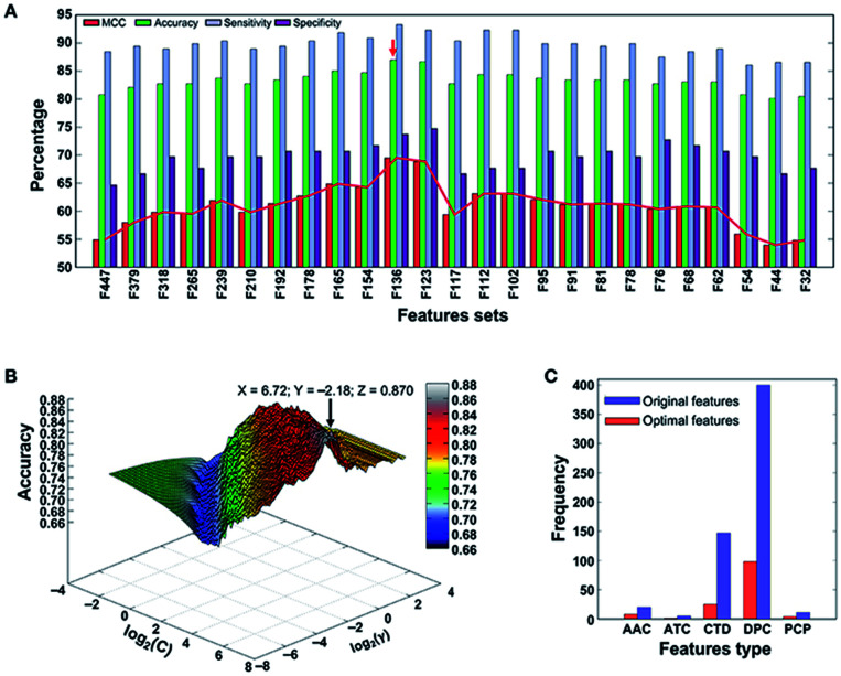
After long-term development, the support vector machine algorithm has already been able to greatly simplify problems, reduce the dimensions of data, and eliminate noise, which shows great generalization ability in unknown samples. Xintao Qiu and colleagues combined SVM and recursive feature elimination to model atmospheric corrosion of materials. This brand new method can extract the most influential factors and build a reliable analyzing model. Also, when selecting corrosion factors in small sample sizes, it greatly outperforms other algorithms in regression and prediction performance.⁵⁸ To detect the molecular functions and biological activities of phage virion proteins, Balachandran Manavalan trained a SVM predicting model with 136 features called PVP-SVM. The performance of PVP-SVM was consistent in both the training and testing datasets, and the cross-validation showed that the accuracy of PVP-SVM is 0.870, which is higher than that of any other control SVM predictors⁵⁹ (Fig. 5).

Fig. 5. (a) Performance of SVM-based classifiers in distinguishing between PVPs and non-PVPs. The red arrow denotes the final selected model. (b) Classification accuracy of the final selected model. (c) Distribution of each feature type in the optimal feature set (136 features) and original feature set (583 features).⁵⁹.

Currently, SVM is also making good progress in the medical field. Manfred K. Warmuth's team used SVM to classify and screen compounds related to a target drug and successfully identify the most satisfactory drug in the screening. In this procedure, the classification characteristics of SVM could effectively judge the correlation between the compound and the target, and it showed very good accuracy in the final test.⁶⁰

3.4. Decision tree and random forest

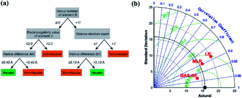
The decision tree^61–63 is a type of supervised learning. When a decision tree is generated, the source dataset (which constitutes the root node) is split into several subsets (which constitute the successor children) according to a series of splitting rules based on classification features. By repeating this procedure, a decision tree grows (Fig. 6a). The decision tree is also used in classification problems; however, it still has some shortcomings, such as overfitting and generalizing weakness. Therefore, researchers created the random forest algorithm, lifting tree algorithm, and many other algorithms based on the decision tree. The random forest algorithm^64,65 is a classifier composed of multiple decision trees. The random forest solves the problems of a single decision tree by the voting mechanism of multiple decision trees, which greatly improves its generalizing ability.

Fig. 6. (a) Schematic of a single decision tree.³² (b) Taylor diagram of different models for UCS prediction.⁶⁹.

In an experiment by Anton O. Oliynyk and coworkers,³² they attempted to synthesize AB₂C Heusler compounds using the random forest algorithm.^66,67 By averaging the predictions of these decision trees, the random forest aggregates the different trends of each tree, which results in a complex and stable model. They selected two gallium-containing compounds (MRu₂Ga and RuM₂Ga (M = Ti–Ni)) to test its predictive ability. After the prediction, they were considered to have more than 60% probability of forming a Heusler compound, and Co₂RuGa had a higher probability of around 92%.³² Derek T. Ahneman and colleagues attempted to predict the Buchwald–Hartwig amination reaction against Pd catalysis, the root mean square error (RMSE) of the test set of the random forest mode was 7.8%, which was much better than those of kernel ridge regression (KRR), support vector machine, Bayes generalized linear model and single layer neural network algorithms.⁶⁸ In another case, Junfei Zhang and his colleagues used a beetle antennae search algorithm-based random forest (BAS-RF) method to detect the uniaxial compressive strength (UCS) of lightweight self-compacting concrete. The results showed that this algorithm has high predictive accuracy, indicated by the high correlation coefficient of 0.97. In Fig. 6b, it is clear that BAS-RF has a lower root-mean-square error value and a higher correlation coefficient than multiple linear regression (MLR) and logistic regression (LR), indicating better performance.⁶⁹

3.5. Artificial neural network (ANN)

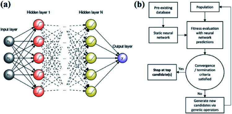
An artificial neural network,^70,71 which is constructed by neurons, is a type of ML algorithm that simulates biological cranial nerves. The neural network dates back to 1949, when a Canadian psychologist, Donald Hebb, developed a theory of learning known as Hebbian learning.⁷² However, it was not until nearly two decades later that ANN was largely developed. In the early period of ANN, a single-layer neural network was first proposed. However, due to some of its specific limitations, researchers generally turned to multiple-layer neural networks in later studies; these networks consist of an input layer, hidden layer and output layer. Fig. 7a shows a typical example of a multiple layer neural network. Neural network algorithms can analyze problems efficiently by nonlinear complex interactions between neurons. It has been confirmed that ANN is very useful in the following three situations:³⁵

Fig. 7. (a) An example of a feed-forward ANN with N hidden layers and a single neuron in the output layer.⁸⁰ (b) Schematic of an ANN-evaluated genetic algorithm.⁷⁴.

1. The number of samples or experiments is very large.

2. There is not much a priori information about the dataset.

3. In the above case, the target is only predicted within the model domain.

Edward O. Pyzer-Knapp used a special form of neural network called a “multilayer perceptron” to discover new compounds. Edward and his colleagues used the multilayer perceptron to continuously filter datasets, eliminate data with small correlations after each iteration, and then place the remaining data into the next round of screening, thereby locking the target compound while minimizing computational effort.¹⁸ Tian Zhang and colleagues proposed a novel approach of using ANN to realize spectrum prediction, performance optimization and inverse design for a plasmonic waveguide-coupled with cavities structure.⁷³ Tarak Patra and colleagues built a neural network-biased genetic algorithm that can discover materials with extremal properties in the absence of pre-existing data. It was shown to outperform both a nonbiased genetic algorithm and a neural-network-evaluated genetic algorithm based on a pre-existing dataset in a number of test applications. Fig. 7b shows a schematic of the ANN-evaluated genetic algorithm applied in this experiment⁷⁴ (Fig. 7b). Tian Xie and Jeffrey C. Grossman developed a crystal graph convolutional neural network to learn material properties from the connection of crystal atoms and accelerate the design of crystalline materials. This neural network could realize the design of crystal materials with very high accuracy. In practical application, it successfully discovered 33 perovskites in the dataset, and it significantly reduced the search space of high throughput screening.⁷⁵

Neural network algorithms are also used for drug development. In the past few decades, the connection of computing technology and drug development has become increasingly close.⁷⁶ At present, many ML algorithms such as neural networks have already been applied in the field of drug design; they can help predict the structure and biological activity of target compounds and specifically study their pharmacokinetics and toxicology.^77–79

3.6. Deep learning

The idea of deep learning^81,82 originated from research of a multiple-layer ANN. In some ways, deep learning is a branch subject of ANN. However, deep learning has already developed a series of research ideas and methods of its own. It is a method of characterizing learning based on data. As a new field in machine learning, deep learning aims to build a neural network that mimics the human brain to analyze data. In some ways, deep learning is similar to a neural network with multiple layers. A deep learning algorithm can extract the underlying features in the underlying network and combine them with the underlying features in the upper network layers to obtain more abstract high-level features. As the number of neural network layers increases, the features obtained by the algorithm will be more abstract. At the top level, the final advanced features are combined, enabling the neural network to correctly recognize an object. For example, for a square, the deep learning algorithm will first extract features such as “four line segments” and “four right angles”. As the neural network layer increases, the algorithm will obtain abstract features such as “four line segments connected” and “four line segments of equal length”. Finally, these features will be combined and the algorithm will correctly recognize the square. One thing to note here is that unlike more primitive machine learning methods, deep learning does not require the researcher to manually implement the feature engineering processing of the input data; instead, the algorithm will self-adjust and choose suitable features independently in continuous learning. This can be considered as a major advancement in machine learning.

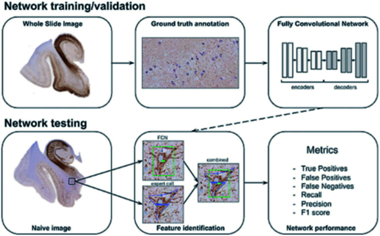
The idea of deep learning was proposed in 2006. After more than a decade of research, many important algorithms have been developed, such as convolutional neural networks (CNNs), automatic encoder, sparse coding, restricted Boltzmann machine (RBM), deep belief networks (DBN), and recurrent neural networks (RNNs). Currently, deep learning is being widely used in many fields, such as computer vision, image recognition and natural language recognition. For example, convolutional neural networks are used to detect corrosion in many facilities;⁸³ also, Maxim Signaevsky and his coworkers proposed the use of deep learning algorithms to judge the accumulation of the abnormal protein TAU to help diagnose neurodegenerative diseases.⁸⁴Fig. 8 shows how they extracted image patches for network training and tested the robustness and reliability of the network with naïve images. Izhar Wallach used deep learning to predict the biological activity of small molecules in drug discovery.⁸⁵ Overall, as a new machine learning method, deep learning has excellent development prospects.

Fig. 8. Schematic overview of data annotation and the deep learning pipeline in neurodegenerative disease diagnosis.⁸⁴.

Table 2 summarises some basic algorithms used in material science. In addition to the algorithms mentioned above, many other methods have been experimentally tested. Generally, practical processes are often based on supervised learning, in which researchers usually combine personal experience and ML algorithms. Narrowing down to a specific project, the research idea is not limited to a certain method, and algorithms are also selected and designed individually according to the practical situation.

An overview of some basic machine learning algorithms.

Algorithm	Brief introduction	Advantages	Disadvantages	Representative applications
Regression analysis	It can find regression equations and predict dependent variables	Deeply developed and widely used in many occasions	Needs large amounts of data and may cause overfitting in practical applications	Machine learning with systematic density-functional theory calculations: application to melting temperatures of single-and binary-component solids
Naïve Bayes classifier	It can classify data into several categories following the highest possibility	Only a small amount of data is needed to obtain essential parameters	The feature independence hypothesis is not always accurate	A naïve-Bayes classifier for damage detection in engineering materials
Support vector machine	SVM can find a hyperplane to divide a group of points into two categories	It has great generalization ability and can properly handle high-dimension datasets	SVM is not very appropriate for multiple classification problems	PVP-SVM: sequence-based prediction of phage virion proteins using a support vector machine
Decision tree and random forest	By splitting source datasets into several subsets, all data will be judged and classified	The calculating processes are easy to comprehend. Also, it can handle large amounts of data	It is difficult to obtain a high-performance decision tree or a random forest. Also, the overfitting problem may occur	High-throughput machine-learning-driven synthesis of full-Heusler compounds
Artificial neural network	By imitating neuron activities, ANN can automatically find underlying patterns in inputs	ANN has great self-improving ability, great robustness and high fault tolerance	Its inner calculation progresses are very difficult to understand	Learning from the Harvard Clean Energy Project: the use of neural networks to accelerate materials discovery
Deep learning	Originated from ANN. It aims to build a neural network to analyze data by imitating the human brain	It has the best self-adjusting and self-improving abilities compared with other ML methods	As a new trend in ML, deep learning has not yet been well studied. Many defects are still unclear	Artificial intelligence in neuropathology: deep learning-based assessment of tauopathy

4. Cross-validation

The main goal of machine learning is material prediction; therefore, it is necessary to test the quality of the predicting model. If the model is not flexible enough or the volume of input data is not sufficient enough to find the appropriate physical chemical rules, the predicting results will not be reliable. If the model is too complex, the results may be over-fitted. In order to avoid these possible risks, researchers must verify the correctness and reliability of predicting model, and the key to verification is using unknown data to test the model and determine its accuracy. Here, we will briefly introduce several methods of cross-validation. Additionally, it is important to know that cross-validation is reliable only when the training sets and validation sets can represent the entire dataset.⁸⁶

4.1. Average cross-validation on multiple hold-out estimates

The average cross-validation method⁸⁷ was developed on the basis of the holdout estimation method. The accuracy of the original holdout validation method was usually lower than expected. Therefore, after improvement by Geisser, it was transformed into the average cross-validation method. The average cross-validation method can avoid the random effects caused by one-time division that may occur in the original method. However, if the volume of data continues to increase, it will lead to very large computational cost and unaffordable computational complexity.^88,89

4.2. Leave-p-out cross-validation and leave-one-out cross-validation

In order to reduce computational complexity, researchers proposed leave-p-out cross validation (LPO).^90,91 In holdout estimation, the number of subsets for validating a calculation is 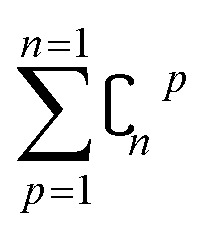; however, in LPO, this number decreases to 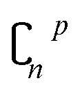. In this way, the computational complexity is successfully reduced; however, the high computational costs caused by very large amounts of data are still unacceptable.

Leave-one-out cross validation (LOO)⁹² is a special form of leave-p-out cross validation. In LOO, the number p = 1, which decreases the number of subsets from to n. After years of development, it is now widely used due to its decreased volume of computation. However, LOO still has some defects. It may underestimate the predicting error⁹³ and may also lead to overfitting.⁹⁴

4.3. Repeated learning test cross-validation

The repeated learning test (RTL) cross-validation⁹⁵ was introduced by Breiman and was further studied by Burman and Zhang. It divides only a part of dataset instead of the whole dataset.^95–98 Compared with previous verification methods, the computational complexity of RLT is significantly reduced.

4.4. Monte Carlo cross-validation

The Monte Carlo cross-validation (MCCV)^99,100 is similar to RLT but is easier to operate. The MCCV leaves out some samples every time for validation, then repeats this procedure many times. Khaled Haddad attempted to verify the regional hydrological regression model by LOO and MCCV. Compared with LOO, MCCV can select more simplified models, and it can also better estimate the predicting ability of models.¹⁰¹

4.5. K-fold cross-validation

K-fold cross-validation¹⁰² has been proposed as an alternative solution for LOO. It is now the simplest and most widely used generalization error estimation method. The most obvious advantage is that only K times calculations are required, and its calculation cost is far less than the cost of LOO or LPO. However, it should be noted that when the K number is not large, this method may have larger biases.⁹⁵

4.6. Bootstrap cross-validation

Because K-fold cross-validation tends to have great variations in the cases of small volumes of sample data, researchers proposed bootstrap cross-validation (BCV).^95,103 Compared with traditional validation methods, BCV has less variability and fewer biases under a small amount of samples. However, it must be noted that the calculation amount of BCV will increase sharply under large samples; therefore, it is not recommended to use BCV in this situation.¹⁰³

All the analysis shows many different cross validation methods and their unique characteristics. As we can see, more research is needed to further improve the cross-validation methods.^98,104,105

5. Assisting DFT calculations with machine learning

In this section, we will introduce a novel idea of assisting traditional DFT calculations with ML. The first part will thoroughly state the theoretical basis of this idea and how it works in experiments. In the second part, we will discuss several cases of applying this new idea and show its great effects and prospects.

5.1. The theoretical basis of assisting DFT with ML

Density functional theory (DFT) is a quantum mechanical method for studying the electronic structures of multi-electron systems. It has been widely used in material science and computational chemistry because of its high calculating accuracy. However, some defects of DFT are quite obvious in practical application: the calculation method is overly complicated, the calculation processes occupy large amounts of computing resources, and the ability of DFT itself is limited by the exchange function that describes the non-classical interaction between electrons. These problems are even more serious when handling complex materials. At present, the new material discovery mode based on DFT may be considered to be too expensive with respect to computing costs and experimental costs. Therefore, researchers are attempting to assist or partially replace DFT with machine learning in material discovery procedures. As an auxiliary method, machine learning can help avoid the defects of traditional DFT calculation and improve the experimental results in practical applications. In fact, it has been proved that when the amount of data is sufficient, machine learning can reproduce the properties of DFT calculations, and the deviation from the DFT values is smaller than the deviation of DFT calculation results from experimental values.^80,106,107 Also, when faced with small amounts of data, researchers should focus on the dataset itself and attempt to construct a more delicate and highly efficient dataset to eliminate this deviation. Although Daniel C. Elton has proved that it is possible to achieve high accuracy using a small amount of data, the amount of data is still a limitation of ML methods. There are still many unclear details in this field, and more essential research is need.³¹

From the theoretical point of view, the study by Rampi Ramprasad revealed an important phenomenon that machine learning based on data prediction is actually consistent with the nature of scientific processes: it starts with basic observations (data analysis), followed by intuition (predictive) and finally by building a quantitative theory (feedback corrections and learning) that explains the observational phenomena. Because of this theoretical support, it is reasonable to assist DFT calculations with machine learning.⁹

Specific to the actual research methods, first, researchers need to represent the various materials in the dataset digitally. Each material (input) should be represented as a string of numbers, which is called the fingerprint vector. The highly distinctive fingerprint vectors are organized by the descriptors and represent the features of the material. Secondly, researchers must establish mapping between input and target features, and this mapping relation is also totally digitized. Many of the ML algorithms mentioned before can be applied here. When this mapping is established, researchers have the objective conditions to predict new materials with similar materials.

In addition, complete digital mapping means that researchers do not need to consider complex physicochemical relationships when discovering new materials. Because the original materials (input) have all the above physicochemical properties, correspondingly, the target materials naturally conform to those physicochemical properties. This is an essential theory that focuses on data, and it can greatly reduce the computational pressure of existing methods.

5.2. Practical application cases

Many researchers are already involved in this work. For example, I. E. Castelli and K. W. Jacobsen conducted a study about perovskite crystals with the ABO₂N cubic structure. They used machine learning instead of traditional DFT calculation to calculate the tendency of various elements to form perovskites, and they successfully performed simple data manipulation for bandgap evaluation.¹⁰⁸ Ghanshyam Pilania and colleagues attempted to use chemical structures and electron charge density as “fingerprint vectors” to find new material properties. Their results showed same-level accuracy and lower experimental consumption compared with DFT.¹⁰⁹ However, this method has a certain limitation, namely that the maps corresponding to each type of material are totally different and can only be applied to specific types of materials. Under this circumstance, it is necessary to find a special map for each type of material to meet research needs. It is also worth mentioning that Logan Ward attempted to replace the dataset with a set of universal material features, then use the feature set as “fingerprints” to find a broad mapping property for the vast majority. This method can analyze most materials with a general model and avoid calculating a mapping for each material, thus greatly saving research costs. In this research, they selected the random forest algorithm to build the model and then tested it twice. In the first experiment (using a DFT-validated property database to predict new solar cell materials), the model showed excellent performance, with the lowest average absolute error in ten cross-validations. The second experiment (exploring new metal-glass alloys using experimentally measured data on the ability of crystalline compounds to form glass) showed fairly high accuracy of 90.1% in ten cross-validations.¹¹⁰

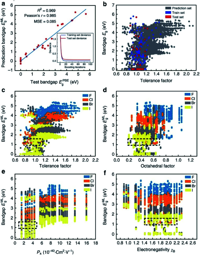
In addition, in one of the most typical cases in the field of assisting DFT with machine learning algorithms, Shuaihua Lu's team used this method to find suitable mixed organic–inorganic calcium–titanium (HOIP) as a new type of photovoltaic material. The researchers used the machine learning method to train the bandgap model and selected four ideal solar cell properties as the measurement indicators; then, they successfully selected six suitable materials from 5158 undetected target compounds. The results are listed in Fig. 9. As the iteration numbers increased, the deviation between the training and testing sets decreased (Fig. 9a). The distribution of the post-predicted bandgap was also very close to the original input sets (Fig. 9b). Other hidden trends and periodicities were also unraveled by data visualization. The results are shown in Fig. 9c–f, which is divided according to the position of the X-site element (F, Cl, Br and I). Different from traditional methods, DFT was only used here to help calculate the most probable target materials rather than all target substances, thus greatly reducing the computational costs.²⁸

Fig. 9. Results and insights from the ML model. (a) The fitting results of the test bandgaps E^PBE_g and predicted bandgaps E^ML_g. (b) Scatter plots of tolerance factors against the bandgaps for the prediction dataset from the trained ML model (the blue, red and dark gray plots represent the training, testing and prediction sets, respectively). Data visualization of predicted bandgaps for all possible HOIPs (each color represents a class of halogen perovskites) with the (c) tolerance factor, (d) octahedral factor, (e) ionic polarizability for the A-site ions, and (f) electronegativity of the B-site ions. The dotted boxes represent the most appropriate range for each feature.²⁸.

In practical application, the experimental accuracy of ML can also be maintained. For example, Prasanna Balachandran and colleagues constructed a new ML material discovery method by constructing orbital radii based on data and applied this method from relatively simple AB compounds to more electronically complex RM intermetallic compounds. The results showed great agreement of the classification rules extracted from both ML and DFT calculations.¹¹¹ In another case, Daniele Dragoni constructed a Gaussian approximation potential (GAP) model and trained it with DFT data from 150k atoms. After finishing the construction, the researchers verified the accuracy of the model with another group of DFT data. The results show that this model can reproduce DFT calculations and maintain very high accuracy. For example, the value of the bulk modulus by GAP is 198.2, while that by DFT is 199.8 ± 0.1 (ref. 7). The deviation between these two methods is quite small.¹¹² Furthermore, many other cases have proved the high accuracy of the ML method; for example, Felix Faber used 13 different quantum properties from over 117k atoms to test the accuracy of ML and DFT calculations, and it was shown that ML can definitely reach the accuracy of DFT.¹¹³ Albert P. Bartók and coworkers built a ML model that can distinguish active and inactive protein ligands with more than 99% reliability. This experience-dependent method could reach the same level of accuracy as DFT with quite low cost.¹¹⁴ Ryosuke Jinnouchi and Ryoji Asahi attempted to use ML to detect the catalytic activity of nanoparticles with DFT data on single crystals. The accuracy could also meet the expectations of practical application.¹¹⁵

In addition to all the practical examples above, researchers have attempted to optimize the DFT calculation process by ML. Solving the Kohn–Sham equation is a necessary step in the DFT calculation process, and this very step is also the most time-consuming part of the DFT calculation process. In this field, John C. Snyder and Felix Brockherde have already obtained some significant results.^116,117 These results show that taking advantage of the flexibility and efficiency of ML can highly reduce the computational cost of DFT, which can decrease the calculation time and increase the calculation speed.

From these examples, we can see that the methods and ideas of ML have brought great convenience to material research. Because ML is a pure data operation, the computer can quickly determine all physical and chemical rules using sufficient data and the correct algorithm whether they are hidden or discovered, which may someday back-feed theoretical chemistry.¹¹⁸ The method of ML combined with data operation has less computational complexity and computational cost compared with traditional DFT calculation. However, the accuracy of this new idea is currently below expectations. Ying Zhang and his team have attempted to introduce additional parameters into the calculation to improve the accuracy of the models; however, the best models still do not have the high accuracy of traditional DFT calculations.³⁶ From this point of view, although the idea of ML combined with data operation can bring great changes to current material science research, there are also defects to be overcome.

6. Artificial intelligence-assisted new material development

Artificial intelligence (AI) is the subject of computer science simulating human intelligence. Since its birth in 1950, it has gone through many ups and downs. Currently, due to the development of big data and computer technology, the theoretical system of AI is hugely enriched. AI now has many subfields, such as data mining, computer vision, and machine learning. Moreover, it has shown great potential and ability in material science, and it is widely used in material design, corrosion detection, material screening and many other fields of material science. In this section, we will introduce some subfields of AI and their applications in material science.¹¹⁹

6.1. Inverse design for desired compounds

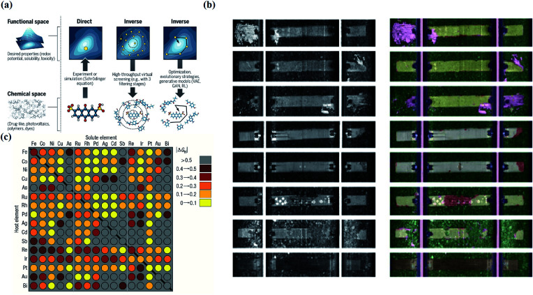
Inverse design aims to find materials with desired particular or material functionalities. Inverse design is significantly different from forward development. The traditional forward design is to obtain the target materials through experiments and then further judge the functionalities of the materials. Inverse design has a more obvious goal-oriented characteristic. It starts from the desired properties and ends in chemical space. The difference is illustrated in Fig. 10a. However, inverse design faces a very obvious problem. Because the aim of inverse design is to find suitable materials based on functionalities, we can consider this process as starting from specific conditions to find possible solutions among a large range of candidate materials and material combinations. According to current research, the optimal solution may or may not exist, and there may be one or more solutions. However, in the process of searching for the optimal solution, the number of candidates waiting for analysis will also increase tremendously. For example, for pharmacologically relevant small molecules, the number of structures is considered to be nearly 10⁶⁰.¹²⁰ Data of this volume cannot be verified manually. Therefore, we introduce ML in this process to help researchers with the analysis.

Fig. 10. (a) Schematic of different approaches toward molecular design. Inverse design starts from desired properties and ends in chemical space, unlike the direct approach, which leads from chemical space to the desired properties.¹²¹ (b) Computer vision analysis of pictures to detect rail defects.¹²³ (c) Computational high-throughput screening for |ΔG_H| on 256 pure metals and surface alloys. The rows indicate the identities of the pure metal substrates, the columns indicate the identities of the solutes embedded in the surface layers of the substrates, and the diagonal of the plot corresponds to the hydrogen adsorption free energy of the pure metals.¹³¹.

A basic idea of inverse design originates from high-throughput virtual screening. This is a data-driven experimental idea. There are many successful application examples. For example, Benjamin Sanchez-Lengeling¹²¹ and Alán Aspuru-Guzik once thoroughly explored the inverse design method. From the current point of view, the research idea and implementation method of inverse design are quite diversiform; however, they are still not mature. Some specific procedures, such as the digital representation of molecules, the selection of ML methods, and the design of inverse design tools, still need further study.¹²¹

6.2. Computer vision for material-picture analysis

Computer vision is defined as an artificial intelligence system that can extract information from images or multidimensional data. Computer vision technology originated very early; however, it did not receive attention or development until the 1970s, when the ability of computers sufficiently improved to handle large-scale data such as images. For example, in the late 1980s, Y. LeCun used the letters in the US postal system as an example and applied computer vision technology to analyze and determine the handwritten zip codes on letters.¹²² Today, computer vision has become an interdisciplinary technology that is widely used in various related fields, and it has also been applied in many subfields of material science. In material science, computer vision can analyze unclear or unknown material properties from enormous amounts of figures, which can greatly help scientists to understand the physical/chemical properties and inner relationships of similar materials. In this way, scientists can better design and construct novel target materials. Examples include detecting corrosion of concrete railway ties by analyzing rail pictures¹²³ and exploring the particle morphologies and surface textures of powders by analyzing microstructure pictures of the powders for additive manufacturing processes.¹²⁴ In the first case, we can see that the computer divides every tie in four pictures and separately evaluates them to detect the conditions of crumbling and chipping (Fig. 10b). In the last case, researchers used a “bag of visual words” method, and the final classification accuracy was 80–85%. In another typical case, M. X. Bastidas-Rodriguez used machine learning algorithms (ANN and SVM) to classify the fracture of metal materials for failure analysis. The results showed that the performance of the ANN application was slightly stronger than that of SVM, and the highest accuracy percentage was 84.95%.¹²⁵ In addition, some researchers have further explored the theory of computer vision. For example, Brian L. DeCost and Elizabeth A. Holm attempted to develop a general method to find useful characteristics and relationships of massive microstructures in large and diverse microstructural image databases. In this research, a “visual dictionary” method was created to detect the characteristics of images by extracting meaningful details and features in pictures to construct “visual words” and by expressing the pictures as the probability distribution of the visual words.¹²⁶ Moreover, computer vision plays an important role in material classification. For example, Hua Chen and colleagues proposed a polarization phase-based computer vision method for material classification according to intrinsic electrical conductivity. This method is computationally efficient and can be achieved with existing image technology.¹²⁷

6.3. High-throughput screening and big data in material discovery

High-throughput screening in the field of novel material discovery uses tremendous volumes of data to perform computational tasks to detect material properties and design target materials. Big data can be defined as a research method that extracts information and detects relationships from extraordinarily large datasets. These two ideas are now often used in novel material discovery.^128–130 Researchers collect very large volumes of data about target materials and use high-throughput screening to analyze the properties of the materials or the possibility of synthetizing target materials. Considering the need for data when applying ML, these two methods have literally become the foundations of the novel material discovery field. There are many cases to prove this; for example, Courtney R. Thomas's team built high-throughput screening to estimate the safety, nanotoxicology, ecotoxicology, environmental assessment and other properties of engineered nanomaterials.¹³¹ Jeff Greeley and his colleagues used DFT-based high-throughput screening to estimate the activity of over 700 binary surface alloys to find an appropriate electro-catalyst for the hydrogen evolution reaction, and they successfully identified BiPt as the desired target material¹³² (Fig. 10). Kirill Sliozberg's team created an automated optical scanning droplet cell for high-throughput screening and high-throughput preparation. They applied this tool in the evaluation of thin-film Ti–W–O and thin-film Fe–W–O to seek efficient semiconductors.^133,134 In another case, Ankit Agrawal and Alok Choudhary systemically described the important role currently played by big data in materials informatics.¹³⁵

In addition to ML, other AI algorithms are widely used in the field of novel material discovery, and there are numerous cases showing the importance, effects, and development prospects of AI. In summary, AI has strong effects and a bright future in materials science; however, it still needs further development.

7. Prospects and conclusion

Led by MGI, the era of data-driven material discovery has arrived. Over the past decades, with the development of computing technology, the progress of AI science, and abundant experimental results, this new material discovery method has generally become a research paradigm. As the research deepens, it is showing many advancing abilities, such as low experimental consumption, low time consumption, high generalizing ability and high density analysis. Currently, it is used in basic chemistry, pharmaceutical science and materials science, such as terahertz spectral analysis and recognition,¹³⁶ prediction of the melting temperatures of binary compounds⁴⁸ and the band gap energies of certain crystals,^137,138 and analysis of complex reaction networks.¹³⁹

However, this method also has certain defects. The accuracy of the results highly depends on the quality of the data and algorithms. Defects such as computing consumption, reliability of algorithms and dependence of data must be overcome. Measures must be taken to improve this method, including establishing reliable databases, enhancing the combination of ML with other material theories, and exploring other new material research methods, such as inverse design. Currently, we are making progress in this field and gradually improving this method. With the development of research, more important effects will be revealed.

Conflicts of interest

There are no conflicts to declare.

Biographies

Biography

Jiazhen Cai.

Jiazhen Cai is a bachelor's degree candidate at the School of Electronic Engineering at Beijing University of Posts and Telecommunications. He joined professor Wei's group in the summer of 2018, and he is especially interested in machine learning.

Biography

Jing Wei.

Jing Wei received her PhD from Peking University in 2017. She is now an associate research fellow at Beijing Institute of Technology. Her research interests focus on semiconductor materials and their optoelectronic devices, information functional materials and devices, and computational materials science.