A New Context Tree Inference Algorithm for Variable Length Markov Chain Model with Applications to Biological Sequence Analyses

Abstract

The statistical inference of high-order Markov chains (MCs) for biological sequences is vital for molecular sequence analyses but can be hindered by the high dimensionality of free parameters. In the seminal article by Bühlmann and Wyner, variable length Markov chain (VLMC) model was proposed to embed the full-order MC in a sparse structured context tree. In the key procedure of tree pruning of their proposed context algorithm, the word count-based statistic for each branch was defined and compared with a fixed cutoff threshold calculated from a common chi-square distribution to prune the branch of the context tree. In this study, we find that the word counts for each branch are highly intercorrelated, resulting in non-negligible effects on the distribution of the statistic of interest. We demonstrate that the inferred context tree based on the original context algorithm by Bühlmann and Wyner, which uses a fixed cutoff threshold based on a common chi-square distribution, can be systematically biased and error prone. We denote the original context algorithm as VLMC-Biased (VLMC-B). To solve this problem, we propose a new context tree inference algorithm using an adaptive tree-pruning scheme, termed VLMC-Consistent (VLMC-C). The VLMC-C is founded on the consistent branch-specific mixed chi-square distributions calculated based on asymptotic normal distribution of multiple word patterns. We validate our theoretical branch-specific asymptotic distribution using simulated data. We compare VLMC-C with VLMC-B on context tree inference using both simulated and real genome sequence data and demonstrate that VLMC-C outperforms VLMC-B for both context tree reconstruction accuracy and model compression capacity.

1. INTRODUCTION

Markov chains (MCs) have been widely applied to molecular sequence analyses. For example, MCs provide a natural way to study the dependencies between the bases of DNA sequences (Blaisdell, 1985), the enrichment and depletion of certain word patterns (Pevzner et al., 1989), prediction of the occurrences of long word patterns from short patterns (Arnold et al., 1988; Hong, 1990), and detecting signals in introns (Avery, 1987). The statistical inference of MCs has been established (Billingsley, 1961). In particular, the statistical estimation of the finite-state MC transition probabilities from long DNA sequences has been extensively studied [see the surveys by Reinert et al. (2000, 2005)]. The estimation of MC transition probabilities from next-generation sequencing reads data has been studied in the works by Ren et al. (2016) and Wan et al. (2020).

The full MCs with a high but fixed finite order provide one of the most general ways to model molecular sequences. However, the estimation of high-order MCs suffers from the curse of dimensionality since the number of free parameters of the full MCs will grow exponentially with the increasing of the order k [e.g., for a MC with a finite-state space $X$, the number of free parameters is $\left(\left|X\right|-1\right)|X{|}^k$, where $\left|X\right|$ is the cardinality of $X$]. Therefore, in practice, inferences of high-order full MCs are limited by the paucity of the data.

To settle the curse of dimensionality problem raised by fitting high-order MC models, the pioneer work by Rissanen (1983) introduced a universal data compression system, which embeds the full MC of order k in a hierarchal structure of a variable length memory. In their seminal article, Bühlmann and Wyner (1999) recasted the concept of universal data compression system as the framework of variable length Markov chains (VLMCs). The processes of VLMC are still Markovian of high order, but with variable length memory: assume that the stationary process ${\left\{X_t\right\}}_{t\in \mathbb{Z}}$ takes values in a finite categorical state space $X$ and denote the subsequence $X_m^n=X_n,X_{n-1},\cdots ,X_m\left(m<n\right)$, a stationary full MC of order k is characterized by the time-homogeneous transition probabilities $P\left(X_t=x_t|X_{-\infty }^{t-1}=x_{-\infty }^{t-1}\right)=P\left(X_t=x_t|X_{t-k}^{t-1}=x_{t-k}^{t-1}\right)$, while the transition probabilities of VLMC are formulated as $P\left(X_t=x_t|X_{-\infty }^{t-1}=x_{-\infty }^{t-1}\right)=P\left(X_t=x_t|X_{t-l}^{t-1}=x_{t-l}^{t-1}\right)$, where the variable number of the lagged value l depends on the actual states of $x_{-\infty }^{t-1}$, and the $x_{t-l}^{t-1}$ is called the context of X_t.

From an algorithmic view, VLMC represents a minimal state space of high-order MC as a context tree, which is sparser than the full context (see the definition in Section 2.2). To infer VLMC from data, Bühlmann and Wyner (1999) proposed the context algorithm to construct the context tree. As we will show later that the context tree inferred by the context algorithm can be systematically biased, we therefore denote the original context algorithm as VLMC-Biased (VLMC-B). VLMC-B mainly contains two steps as follows: (1) first, it constructs a large tree representing an overfitted context tree, or an overestimated VLMC model; (2) then, it prunes nodes of the context tree from bottom up. In the tree-pruning procedure, a branch-specific statistic ${\Delta }_{wu}$ based on word (of the context) counts is defined to measure the difference between the distributions before and after pruning the node u from branch wu.

Once ${\Delta }_{wu}$ is smaller than a fixed cutoff value, the node u would be pruned from the tree. The choice of fixed cutoff value in pruning process is essential: a larger cutoff value will lead to a more conservative estimated tree and vice versa. Bühlmann and Wyner (1999) and Mächler and Bühlmann (2004) recognized ${\Delta }_{wu}$ as the chi-square approximation of log-likelihood ratio test statistic and thus selected the cutoff threshold based on the common chi-square distribution ${\chi }_{\left|X\right|-1}^2$, which underlyingly assumed that the word counts in the statistic are independent. However, the observation nucleotides ${\left\{X_t\right\}}_{t\in \mathbb{Z}}$ are generally dependent on sequences. Besides, the word counts in ${\Delta }_{wu}$ are actually counts for overlapping occurrences of words; thus, dependency is induced due to the overlaps among words. We show that the dependency of word counts is non-negligible, making branch-specific statistic ${\Delta }_{wu}$ deviate from the common chi-square distribution with $\left|X\right|-1$ degrees of freedom.

In this article, we study the word count statistics for VLMC inference and prove the asymptotic distribution of ${\Delta }_{wu}$, with a focus on applications in molecular sequence analyses. The statistical and mathematical properties of word counts in sequence play vital roles in many fields, especially in the study of biological sequence analyses. The statistical and probabilistic foundations of biological sequence analyses have been presented by Waterman (1995) and Reinert et al. (2000). A basic statistical study of sequence involves counting the frequency of a given word, which is a naive but natural problem in practical applications.

The occurrences of words in sequence depend not only on their lengths but also on the ways of counting, which leads to overlapping and nonoverlapping occurrences. For overlapping occurrences, even if the letters in sequence are independent and identically distributed, the random indicators of word occurrences are generally dependent due to overlapping. Without loss of generality, we assume the categorical space $X=\left\{A,C,G,T\right\}$ as in the genome sequence analyses. If a word $w=ACAC$ occurs at position i in the sequence, then it is impossible for w to occur at position $i+1$, and another occurrence of w is more likely to occur at position $i+2$ than the occurrence of w at $i+2$ in the case that w did not occur in position i.

The studies for overlapping word counts aroused great interests of researchers. Gentleman and Mullin (1989) derived the exact probability distribution of frequency of word occurrences for the case that letters are independent and identically distributed and each state occurs at each position randomly with equal probability. Kleffe and Borodovsky (1992) provided the expected frequency of words and found that overlapping properties determine most of the variance and formulated the exact first and second moment of frequency of a given word in sequence generated by a first-order MC.

Lundstrom (1990) derived the covariance matrix of overlapping word counts with multiple patterns as well as its limiting value using $\delta$-method. Prum et al. (1995) studied the asymptotic variance for the difference between counts and its estimated expectation with two estimators of expectation of counts. Huang (2002) provided the error bounds on multivariate normal approximations for word count statistics. Waterman (1995) and Reinert et al. (2000, 2005) summarized the statistical and probabilistic properties of word counts.

In this study, we derive the consistent distribution in tree-pruning process of VLMC-B for each branch-specific statistic based on solid theory of word counts statistics. We prove and demonstrate that, rather than following a common chi-square distribution, the word count-based statistic follows a branch-specific mixed chi-square distribution. We thus propose a new context tree inference algorithm with an adaptive tree-pruning scheme, termed VLMC-Consistent (VLMC-C). The VLMC-C is founded on our consistent branch-specific mixed chi-square distributions calculated from asymptotic normal distribution of multiple word patterns. Meanwhile, VLMC-C also controls the family-wise errors raised by the multiple hypothesis testing of the branches in the context tree. The superiority of our VLMC-C algorithm over VLMC-B proposed by Bühlmann and Wyner (1999) is verified using simulated data and real genome sequence data.

The organization of the article is as follows. In Section 2, we first provide the mathematical formulation of VLMC model (Section 2.1) and the context tree representation of the VLMC model (Section 2.2) and then describe the context algorithm of VLMC-B by Bühlmann and Wyner (1999) (Section 2.3). In Section 3, we provide the details of our VLMC-C method with an adaptive tree-pruning scheme, which reformulates the tree-pruning process for each branch as a hypothesis testing problem: we prove the theorem on the asymptotic distribution of the log-likelihood ratio test statistic (Section 3.1); we then propose our context tree algorithm of VLMC-C using the derived branch-specific mixed chi-square distributions, which are calculated from asymptotic normal distribution of multiple word patterns, and the multiple hypothesis testing (Section 3.2).

In Section 4, we investigate the performance of VLMC-C and compare it with VLMC-B by using simulated data and real biological sequence data. In Section 4.1, we demonstrate using simulated data that the branch-specific statistic follows our theoretical branch-specific mixed chi-square distribution, rather than the common chi-square for all branches. We then compare the VLMC-C algorithm with the VLMC-B algorithm to benchmark their performance on context tree reconstruction (Section 4.2). We demonstrate that the increasing of sequence length will improve the estimation accuracy of VLMC-C, but will worsen the performance of VLMC-B due to its inherent systematic bias (Section 4.3). We apply VLMC-C and VLMC-B on the genomes of Escherichia coli and SARS-CoV-2 and demonstrate that VLMC-C outperforms VLMC-B both in data compression capacity and in balancing model complexity with the likelihood of the sequence (Section 4.4). We conclude the article with discussions (Section 5).

2. VARIABLE LENGTH MARKOV CHAINS

In this section, we first introduce the VLMC model as well as the context algorithm of VLMC-B. The notations and concepts used here mainly follow the work by Bühlmann and Wyner (1999). In this study, we always refer to a MC as a stationary process ${\left\{X_t\right\}}_{t\in \mathbb{Z}}$ with finite order, and taking values from a finite categorical space $X$.

2.1. VLMC model

VLMC is a variant of MC by changing the fixed-length memory of MC to variable length memory. Rather than utilizing all states in the history $x_{-k+1}^0$ of X₁ in a k-th order MC, VLMC compresses the irrelevant states in $x_{-k+1}^0$ and restricts to the minimal state space of MC or the “context” of the sequence, which is the minimal relevant portion of the past that will influence the next outcome. A formal definition of context is defined below.

Definition 1. Let ${\left\{X_t\right\}}_{\in \mathbb{Z}}$ be a stationary process with values $X_t\in X,\left|X\right|<\infty$. Denote $c:X^{\infty }\to X^{\infty }$ as a function, which maps $x_{-\infty }^0\to x_{-l+1}^0$, where l is defined by

$$l=l\left(x_{-\infty }^0\right)=min\left\{k:P\left(X_1=x_1|X_{-\infty }^0=x_{-\infty }^0\right)=P\left(X_1=x_1|X_{-k+1}^0=x_{-k+1}^0\right),\forall x_1\in X\right\},$$

in the case that $l\left(x_{-\infty }^0\right)\equiv 0,\forall x_{-\infty }^0\in X^{\infty }$ corresponds to an independent process. Then, $c\left(\cdot \right)$ is called a context function and for any $t\in \mathbb{Z},c\left(x_{-\infty }^{t-1}\right)$ is called the context for the variable X_t.

The context length of a variable X_t is $l=l\left(x_{-\infty }^{t-1}\right)=\left|c\left(x_{-\infty }^{t-1}\right)\right|$, depending on its history $X_{-\infty }^{t-1}=x_{-\infty }^{t-1}$. Noting that if $l\left(x_{-\infty }^{t-1}\right)\equiv k$ for all $x_{-\infty }^{t-1}\in X^{\infty }$, we obtain a full MC of order k. With the variable length contexts, VLMC can be formulated as follows:

Definition 2. Let ${\left\{X_t\right\}}_{t\in \mathbb{Z}}$ be a stationary process with values $X_t\in X,\left|X\right|<\infty$ and corresponding context function $c\left(\cdot \right)$ as given in Definition 1. Let $0\le k\le \infty$ be the smallest integer such that $\left|c\left(x_{-\infty }^0\right)\right|=l\left(x_{-\infty }^0\right)\le k$ for all $x_{-\infty }^0\in X^{\infty }$, then $c\left(\cdot \right)$ is called a context function of order k. And if $k<\infty ,{\left\{X_t\right\}}_{t\in \mathbb{Z}}$ is called a stationary VLMC of order k.

2.2. The context tree representation of VLMC model

Under the stationary assumption, a VLMC model can be completely specified by its transition probabilities $P\left(X_1=x_1|X_{-\infty }^0=x_{-\infty }^0\right)=P\left(X_1=x_1|c\left(x_{-\infty }^0\right)\right),x_{-\infty }^1\in X^{\infty }$. The states influencing the transition possibilities are determined by the values of context $c\left(x_{-\infty }^0\right)$. Therefore, Bühlmann and Wyner (1999) used a rooted tree structure to depict the context function $c\left(\cdot \right)$ of VLMC.

For a tree representation $\tau$ of a VLMC model, a root is constructed as top node, from which branches grow downward. Each node represents a state from $X$, and thus, each node has $\left|X\right|$ offsprings at most. Therefore, a branch $w=\left\{w_{\left|w\right|},\cdots ,w_1\right\}$ containing nodes from root to leaf node represents a context value of the context function $c\left(\cdot \right)$, that is, $w=c\left(x_{-\infty }^0\right)$.

For example, the tree structure in Figure 1a represents a context function defined as follows:

FIG. 1.

Simulation experiments imply that Delta_approx coincides well with Delta_exact, and statistic Delta_approx follows the branch-specific mixed chi-square distribution. (a) The true context tree of simulated VLMC model. (b) Q-Q plot between Delta_exact and Delta_approx, and Q-Q plot between Delta_approx and ${\chi }^2$ distribution on 13 contexts displayed in (a). Each true context is set as w, and without loss of generality, we set $u=A$ for each context. Red points are Q-Q plot between Delta_approx and mixed chi-square distribution adopted by VLMC-C. Black points are Q-Q plot between Delta_approx and ${\chi }_{\left|X\right|-1}^2$ adopted by VLMC-B. VLMC, variable length Markov chain; VLMC-B, VLMC-Biased; VLMC-C, VLMC-Consistent.

$$c\left(x_{-\infty }^0\right)=\left\{\begin{array}{cc}C,& if{x}_0=C,x_{-\infty }^{-1}arbitrary;\\ G,& if{x}_0=G,x_{-\infty }^{-1}arbitrary;\\ AA,& if{x}_0=A,x_{-1}=A,x_{-\infty }^{-2}arbitrary;\\ AC,& if{x}_0=A,x_{-1}=C,x_{-\infty }^{-2}arbitrary;\\ \cdots & \\ TTA,& if{x}_0=T,x_{-1}=T,x_{-2}=A,x_{-\infty }^{-3}arbitrary;\\ TTC,& if{x}_0=T,x_{-1}=T,x_{-2}=C,x_{-\infty }^{-3}arbitrary;\\ TTG,& if{x}_0=T,x_{-1}=T,x_{-2}=G,x_{-\infty }^{-3}arbitrary;\\ TTT,& if{x}_0=T,x_{-1}=T,x_{-2}=T,x_{-\infty }^{-3}arbitrary.\\ \end{array}\right.$$

2.3. Context algorithm of VLMC-B

In practice, for a sequence $X_1,X_2,\cdots ,X_N$ of a stationary VLMC process, one fundamental goal is to reconstruct the underlying context function $c\left(\cdot \right)$ and to estimate its corresponding transition probabilities. Since the tree representation of VLMC determines its context and vice versa, the estimation of context function $c\left(\cdot \right)$ can be accomplished by estimating a tree representation $\tau$ of VLMC, which can be achieved by various tree estimation methods. Bühlmann and Wyner (1999) introduced a tree inference algorithm, termed as context algorithm (which is denoted as VLMC-B in our study). The main strategy of VLMC-B contains two aspects. One is to construct a large tree representing a redundant context tree, or an overfitted VLMC model, and the other is to prune the overfitted tree with a backward tree-pruning process.

First, we present the notations used in the VLMC-B. For a specific word $w\in {\bigcup }_{m=1}^{\infty }{X}^m$, let

denote the number of occurrences of w in sequence $X_1,X_2,\cdots ,X_N$. The maximum likelihood estimated probability is denoted by

$$\widehat{P}\left(w\right)=\frac{N\left(w\right)}{N},\widehat{P}\left(x|w\right)=\frac{N\left(xw\right)}{N\left(w\right)},x,w\in {\bigcup }_{m=1}^{\infty }{X}^m,$$

where $xw=\left(x_{\left|x\right|},\cdots ,x_1,w_{\left|w\right|},\cdots ,w_1\right)$ is the concatenation of word $x=\left(x_{\left|x\right|},\cdots ,x_1\right)$ and $w=\left(w_{\left|w\right|},\cdots ,w_1\right)$. Based on the estimators, a word count-based statistic is defined for context wu as

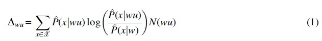
to determine whether to prune away the node $u\in X$ from context wu. The detailed procedures of VLMC-B are described below (Bühlmann and Wyner, 1999).

• 1.Estimate a large tree ${\widehat{\tau }}_0$ to represent an overfitted VLMC model and construct its corresponding context function ${ĉ}_0\left(\cdot \right)$ based on this tree structure. Here, tree ${\widehat{\tau }}_0$ is constructed by containing every branch whose corresponding word occurs at least two times in sequence $X_1,X_2,\cdots ,X_N$.
• 2.Examine every branch of ${\widehat{\tau }}_0$ for pruning. For a context (branch) wu of the current tree ${\widehat{\tau }}_0$,

$$wu=x_{-l+1}^0={ĉ}_0\left(x_{-\infty }^0\right),u=x_{-l+1}\in X,w=x_{-l+2}^0\in {\bigcup }_{m=1}^{\infty }{X}^m,$$

• the branch wu will be pruned to branch w if ${\Delta }_{wu}<K,$ where $K=K_N\sim ClogN,C>2\left|X\right|+4$ is chosen by user. After examining every branch in ${\widehat{\tau }}_0$, a (possibly) smaller tree ${\widehat{\tau }}_1$ is generated and its corresponding context function ${ĉ}_1\left(\cdot \right)$ can be directly obtained.

• 3.Repeat step 2 with estimated tree ${\widehat{\tau }}_i$ until ${\Delta }_{wu}\ge K$ for every branch $wu\in {\bigcup }_{m=1}^{\infty }{X}^m,u\in X$. We denote the final estimated context tree by $\widehat{\tau }$ and its corresponding context function by $ĉ\left(\cdot \right)$.

The choice of a cutoff threshold K in step 2 is essential for the estimation of context tree. A small K will result in a large context tree, even leading to overfitting, while a large cutoff value will result in a conservative context tree and underestimation may occur. Bühlmann and Wyner chose $K=K_N\sim ClogN\left(C>2\left|X\right|+4\right)$ by an asymptotic consideration, which aims to achieve an optimality with respect to some loss function (Bühlmann, 2000). Since the statistic ${\Delta }_{wu}$ can be reformulated as one log-likelihood ratio test statistic, previous studies also suggested setting K as the quantiles of a chi-square distribution with $\left|X\right|-1$ degrees of freedom in practice (Bühlmann and Wyner, 1999; Mächler and Bühlmann, 2004). However, the overlapping word counts in ${\Delta }_{wu}$ is no longer independent induced by the overlaps among words, making the asymptotic distribution of ${\Delta }_{wu}$ deviate from the heuristically expected ${\chi }_{\left|X\right|-1}^2$ distribution. We demonstrate that choosing the fixed K based on ${\chi }_{\left|X\right|-1}^2$ would lead to a systematic bias on tree-pruning decision in the next section.

3. DISTRIBUTION OF WORD COUNT-BASED STATISTIC

Based on the studies for statistical properties of overlapping word counts, we derive the asymptotic distribution theoretically and hence achieve an unbiased tree-pruning decision. In this section, we first reformulate the pruning process for a specific branch wu in VLMC-B as a hypothesis testing problem. We find that the empirical log-likelihood ratio test statistic, termed $\Delta {\prime }_{wu}$, is conceptually equivalent to ${\Delta }_{wu}$ used in VLMC-B and prove that it follows a mixed chi-square distribution under the null hypothesis, rather than ${\chi }_{\left|X\right|-1}^2$ used by VLMC-B. Based on the consistent asymptotic distribution, we design our consistent context algorithm, VLMC-C, for context inference of VLMC.

3.1. Hypothesis testing for tree pruning

The pruning procedure in step 2 of VLMC-B compares a tree with its subtree, which prunes away a leaf node. Since the context tree corresponds to the depending structure in sequence, the comparison of trees can be formulated as the comparison of conditional distributions based on tree structure. Thus, we formulate the tree-pruning process as the following hypothesis testing problem.

Given an observational sequence $S=x_1,x_2,\cdots ,x_N$, an overfitting tree is first constructed as in the VLMC-B algorithm. For a specific branch $wu\left(w\in {\bigcup }_{m=1}^{\infty }{X}^m,u\in X\right)$ of the tree, the hypothesis testing problem to determine whether to prune the branch from wu to w is

$$H_0:P\left(X|wu\right)=P\left(X|w\right),\forall X\in X{H}_1:P\left(X|wu\right)\ne P\left(X|w\right),$$

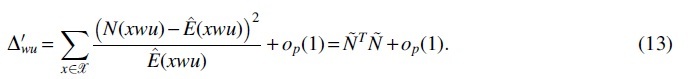
and the log-likelihood ratio test statistic is defined as $\Delta {\prime }_{wu}=-2log\frac{{\widehat{P}}_{H_0}\left(S\right)}{{\widehat{P}}_{H_1}\left(S\right)}$. Since the structures of the two trees before and after pruning node u differ only at the branch wu, the estimated likelihood distribution can be factorized into the products of exactly the same conditional probability terms except for the ones conditioned on wu and w. That is to say, for pruned tree, or under null hypothesis, 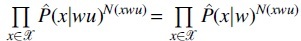holds while it is not the case for unpruned tree, i.e., under the alternative hypothesis. Actually, $\Delta {\prime }_{wu}=2{\Delta }_{wu}$ holds (see Section 6), indicating an equivalence of ${\Delta }_{wu}$ and $\Delta {\prime }_{wu}$ except for a constant multiple.

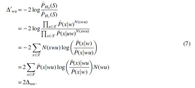
On the basis of studies on difference between overlapping word counts and its estimated expectations (Lundstrom, 1990; Reinert et al., 2000, 2005), we derive the following theorem, indicating the asymptotic normality of the standardized difference of multiple words and proving that $\Delta {\prime }_{wu}$ follows a mixed chi-square distribution under null hypothesis.

Theorem 1. Denote the finite categorical space $X=\left\{v_1,v_2,\cdots ,v_k\right\}$ and $N\left(w\right)$ as the number of overlapping occurrences of word w in a sequence. Then, for a specific branch wu, under the null hypothesis we have

(i)

$$Ñ={\left(\begin{array}{c}\frac{N\left(v_{1}wu\right)-Ê\left(v_{1}wu\right)}{\sqrt{Ê\left(v_{1}wu\right)}}\\ \cdots \\ \frac{N\left(v_{k}wu\right)-Ê\left(v_{k}wu\right)}{\sqrt{Ê\left(v_{k}wu\right)}}\\ \end{array}\right)}_{k\times 1}{\to }^{P}N\left(0,{\tilde{\Sigma }}_{k\times k}\right),$$ (2)

where $Ê\left(vwu\right)=\frac{N\left(vw\right)N\left(wu\right)}{N\left(w\right)}$. And the covariance matrix ${\tilde{\Sigma }}_{k\times k}$ is

$${\tilde{\Sigma }}_{k\times k}\left(v_{i}wu,v_{j}wu\right)=\sqrt{P\left(v_{i}wu\right)P\left(v_{j}wu\right)}\left(\frac{1_{\left\{v_i=v_j\right\}}}{P\left(v_{i}wu\right)}-\frac{1}{P\left(wu\right)}-\frac{1_{\left\{v_i=v_j\right\}}}{P\left(v_{i}w\right)}+\frac{1}{P\left(w\right)}\right),$$ (3)

where $P$ denotes the stationary distribution under the null hypothesis.

(ii)

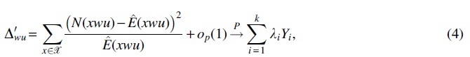
where ${\lambda }_i,i=1,\cdots ,k$ are the eigenvalues of covariance matrix ${\tilde{\Sigma }}_{k\times k}$, Y_i's are independent random variables that follow the chi-square distribution ${\chi }_1^2$ with one degree of freedom, and $o_p\left(1\right)$ denotes a sequence of random variables that converge in probability to zero.

Theorem 1 (i) implies an asymptotic normality for the joint distribution of words of multiple patterns. Theorem 1 (ii) can be directly achieved by (i) and eigendecomposition of the covariance matrix. We present the detailed proof in Section 6.

3.2. The VLMC-C algorithm for context tree inference

We design a context inference algorithm, VLMC-C, based on the consistent testing founded on Theorem 1. The framework of VLMC-C is basically the same as that of VLMC-B, consisting of constructing an initial overestimated context tree and then pruning redundant nodes one by one. We use the same method to construct an initial tree as VLMC-B does.

During tree-pruning process, we apply the breadth-first traversal technique from bottom (leaf nodes) to top (root) when performing hypothesis testing. Strictly speaking, branches with the greatest lengths are first tested, followed by testing the branches in the upper layer, which are shorter. It is worth noting that the significance levels need to be adjusted for multiple hypothesis testing problem. Inspired by the Bonferroni correction method (Dunn, 1961), we set the significance levels of branches in the i-th layer of tree as ${\alpha }_i=\frac{{\alpha }_0}{L_i\times K}$, where L_i is the number of leaves once the pruning process is done for the $\left(i+1\right)$-th layer, K is the order of initial context tree ${\widehat{\tau }}_0$, and ${\alpha }_0$ is a given significance level.

We set ${\alpha }_i$ in this way for three reasons. First, such setting of ${\alpha }_i$ ably controls the family-wise error rate at given level ${\alpha }_0$ (Section 6). Second, the order of testing for branches in the same layer is irrelevant since they have the same ${\alpha }_i$ values. And last but not the least, the ${\alpha }_i$ of a longer branch is smaller, making it inclined to accept the null hypothesis, that is, pruning the branch. This is in line with our intuition during tree-pruning process, that is, a longer branch of a tree is more likely to contain redundant information of lagged states than the shorter ones, thus pruned. The complete computational procedures of VLMC-C algorithm (Algorithms 1 and 2) are shown in Section 6.

4. RESULTS

4.1. Statistic $\Delta {\prime }_{wu}$ follows our derived mixed chi-square distribution

We study the word count statistic $\Delta {\prime }_{wu}$ of VLMC-C and compare it with our derived theoretical mixed chi-square distribution using simulated data. We simulate long DNA sequence based on a third-order VLMC model taking values from $X=\left\{A,C,G,T\right\}$, and the corresponding context tree of the VLMC model consists of 13 contexts (or branches connecting the leaf nodes and the root node in context tree, Fig. 1a). All transition probabilities conditioned on the contexts have none zero values (Table 1). We simulate $R=3000$ sequences independently, and each sequence contains $N=10^5$ letters. The details of simulation procedures are presented in Section 6.

Table 1.

Context-Based Transition Probabilities of Simulated Variable Length Markov Chain in Figure 1a

Context	State
	A	C	G	T
C	1/8	1/4	1/8	1/2
G	1/8	1/4	1/8	1/2
AA	1/10	1/5	3/10	2/5
AC	1/8	1/4	1/8	1/2
AG	1/8	1/4	1/8	1/2
AT	1/8	1/4	1/8	1/2
TA	2/11	5/11	1/11	3/11
TC	2/11	5/11	1/11	3/11
TG	2/11	5/11	1/11	3/11
TTA	1/8	1/4	1/8	1/2
TTC	1/8	1/4	1/8	1/2
TTG	1/8	1/4	1/8	1/2
TTT	3/11	2/11	5/11	1/11

Since the asymptotic normality in Theorem 1 requires the approximation of two statistics (Section 6), denoted as

and

respectively. For each of the R sequences, we calculate the Delta_exact and the Delta_approx, and check whether they are consistent with each other. Since the asymptotic normality holds under null hypothesis, we set w as one of the contexts (corresponding to one of the 13 branches) in Figure 1a to ensure that the null hypothesis holds. And without loss of generality, we set $u=A$ all the time. The true transition probabilities in Table 1 are adopted in calculating the covariance matrix in Theorem 1, rather than using the estimated ones from the simulated sequences. It is clearly shown that the two statistics Delta_exact and Delta_approx are well consistent along the diagonal line of the quantile–quantile plot (Q-Q plot) (the left plot of Fig. 1b).

We then validate the derived theoretical mixed chi-square distribution. For each context w in the context tree and any state $u\in X$ (without loss of generality we still set $u=A$ here), we compute its asymptotic covariance matrix as in Theorem 1 $\left(i\right)$ and obtain the derived asymptotic distribution of $\Delta {\prime }_{wu}$ by eigendecomposition of the covariance matrix. We employ the Q-Q plot to access the difference between the distribution of $\Delta {\prime }_{wu}$ and its corresponding theoretically asymptotic distribution (black points in the right plot of Fig. 1b). Besides, the Q-Q plot for measuring difference between distribution of $\Delta {\prime }_{wu}$ and distribution of ${\chi }_{\left|X\right|-1}^2$, which was adopted by VLMC-B (Bühlmann and Wyner, 1999; Mächler and Bühlmann, 2004), is also presented (red points in the right plot of Fig. 1b). The simulation results imply that the branch-specific statistic $\Delta {\prime }_{wu}$ follows our derived branch-specific distribution of mixed chi-square, rather than the common chi-square distribution ${\chi }_{\left|X\right|-1}^2$.

4.2. VLMC-C outperforms VLMC-B in estimation of context tree

We benchmark the context algorithms of VLMC-C and VLMC-B on context tree reconstruction accuracy using simulated data. The same initial trees for two algorithms are first constructed following the procedures of the VLMC-B software (Mächler and Bühlmann, 2004), where the branches whose corresponding word counts are greater than a predefined count number threshold are retained. For the purpose of saving computation time, we set the threshold as $\sqrt{N}∕\left|X\right|$, where N is the sequence length. It helps to avoid unnecessary hypothesis testing on contexts that are too long to be kept. Besides, it is small enough to build an initial tree containing all real contexts of the simulated VLMC. The other parameters used in VLMC-B are all set to be the default.

When applied to a generated sequence with $10^5$ letters (using the VLMC model in Fig. 1a and Table 1), VLMC-C obtains a more accurate context tree than the tree by VLMC-B (Fig. 2). VLMC-C recovers most of the real contexts (Fig. 2a) except for contexts AC and AG (written in reverse order, i.e., $x_0=A,x_{-1}=CorG$). Besides, it has no redundant nodes of each context (Fig. 2a). VLMC-B however recovers most of nodes in real context tree, except for node G on context AG, it contains large number of redundant lagged states for most contexts, especially in context C and G. It only reconstructs five real contexts accurately ($AA,AC,AT,TTA,TTT$) (Fig. 2b).

FIG. 2.

VLMC-C outperforms VLMC-B in inferring context tree using simulated data. (a) The estimated context tree by VLMC-C. (b) The estimated context tree by VLMC-B. The real context tree of simulated data is presented in Figure 1a.

We further analyze why context AG and AC are missed in the estimated context tree by VLMC-C. We conduct 10 simulation experiments under the same stationary process shown in Figure 1a and Table 1. VLMC-C underestimates context A instead of the real context AC in five simulations, while reconstructing AC successfully in the remaining five simulations. This uncertainty of context AC by VLMC-C indicates the dropping of AC is mainly caused by random errors. VLMC-C fails to reconstruct context AG in all 10 simulations. This is mainly caused by the simulation mechanism of data. The transition probabilities designed are slightly different as $P\left(x|A\right)=\left(0.122,0.244,0.146,0.488\right)\approx P\left(x|AG\right)=\left(0.125,0.25,0.125,0.5\right)$ for $x=A,C,G,T$, making them hard to distinguish at current sequence length.

We also quantify the accuracy of reconstructed trees on the 10 sequences. For each of sequence, we compare the reconstructed trees with the real context tree and calculate the numbers of the false-positive (FP) and false-negative (FN) nodes at each layer of the context tree: an FP event in the hypothesis testing problem corresponds to keeping a redundant node, and an FN event corresponds to cutting off a node by mistake. In each layer of context tree estimated by VLMC-B and VLMC-C, we compute the averaged number, as well as its standard deviation (data in parentheses in Table 2), of FP and FN events based on 10 simulations. It is clearly shown that the estimated context trees by VLMC-C are much more accurate than the trees by VLMC-B (Table 2).

Table 2.

Averaged Numbers of False-Positive and False-Negative Events Among 10 Simulations for the Estimated Context Tree by Variable Length Markov Chain-Biased and Variable Length Markov Chain-Consistent, Respectively

	False positive		False negative
	VLMC-B	VLMC-C	VLMC-B	VLMC-C
Layer 1	$0\left(\pm 0\right)$	$0\left(\pm 0\right)$	$0\left(\pm 0\right)$	$0\left(\pm 0\right)$
Layer 2	$3.7\left(\pm 1.42\right)$	$0\left(\pm 0\right)$	$0.5\left(\pm 0.53\right)$	$1.5\left(\pm 0.53\right)$
Layer 3	$7.4\left(\pm 0.97\right)$	$0\left(\pm 0\right)$	$0\left(\pm 0\right)$	$0\left(\pm 0\right)$
Layer 4	$8.6\left(\pm 1.35\right)$	$0\left(\pm 0\right)$	$0\left(\pm 0\right)$	$0\left(\pm 0\right)$
Layer 5	$6.4\left(\pm 2.27\right)$	$0\left(\pm 0\right)$	$0\left(\pm 0\right)$	$0\left(\pm 0\right)$
Layer 6	$3.3\left(\pm 1.89\right)$	$0\left(\pm 0\right)$	$0\left(\pm 0\right)$	$0\left(\pm 0\right)$
Layer 7	$0.6\left(\pm 0.70\right)$	$0\left(\pm 0\right)$	$0\left(\pm 0\right)$	$0\left(\pm 0\right)$

The numbers in parentheses are their respective corresponding standard deviations. VLMC-C constructs more accurate context trees than those by VLMC-B.

VLMC, variable length Markov chain; VLMC-B, VLMC-Biased; VLMC-C, VLMC-Consistent.

We further validate the performance of VLMC-C and VLMC-B on a fifth-order VLMC model (shown in Fig. 3a and Table 3). On a simulated DNA sequence with $5\times 10^5$ letters, our VLMC-C exactly recovers the underlying true context tree (Fig. 3b). In comparison, VLMC-B outputs a context tree with 15 redundant nodes (Fig. 3c).

FIG. 3.

VLMC-C outperforms VLMC-B in inferring a simulated fifth-order VLMC model. (a) The true underlying context tree structure. (b) The estimated context tree by VLMC-C. (c) The estimated context tree by VLMC-B.

Table 3.

Context-Based Transition Probabilities of Simulated Variable Length Markov Chain in Figure 3a

Context	State
	A	C	G	T
C	1/8	1/4	1/8	1/2
G	1/8	1/4	1/8	1/2
AA	1/10	1/5	3/10	2/5
AC	1/8	1/4	1/8	1/2
AG	1/8	1/4	1/8	1/2
AT	1/8	1/4	1/8	1/2
TA	2/11	5/11	1/11	3/11
TC	2/11	5/11	1/11	3/11
TG	2/11	5/11	1/11	3/11
TTC	1/8	1/4	1/8	1/2
TTG	1/8	1/4	1/8	1/2
TTT	3/11	2/11	5/11	1/11
TTAA	2/11	5/11	1/11	3/11
TTAG	1/8	1/4	1/8	1/2
TTAT	3/11	2/11	5/11	1/11
TTACA	3/11	2/11	5/11	1/11
TTACC	3/11	2/11	5/11	1/11
TTACG	2/11	5/11	1/11	3/11
TTACT	1/8	1/4	1/8	1/2

4.3. Increasing sequence length improves statistical power of VLMC-C

We study the impact of sequence length on the performance of VLMC-C and VLMC-B using four simulated data sets, each of which contains 10 sequences, with the corresponding sequence length $10^3,10^4,10^5$ and $5\times 10^5$, respectively. For each layer of context tree by VLMC-C and VLMC-B, we compute the averaged numbers of FP and FN events based on 10 simulated sequences. We find that when increasing sequence length, both the numbers of FP events and FN events by VLMC-C decrease (Fig. 4a). The sequence length $10^4$ is long enough for VLMC-C to construct a context tree with no redundant nodes, and when sequence length achieves $5\times 10^5$ all contexts are accurately recovered by VLMC-C, even including the node G of context AG, which has been dropped by VLMC-C at the sequence length $10^5$. These results all show that increasing sequence length does help to improve the statistical power of the hypothesis testing in VLMC-C, thus improving the accuracy of VLMC-C.

FIG. 4.

Increasing sequence length has no effect on improving estimation accuracy of VLMC-B while greatly enhance the estimation accuracy of VLMC-C. The averaged numbers of false-positive and false-negative events in each layer of estimated context tree by (a) VLMC-C and (b) VLMC-B using sequences with various lengths. L_k indicates the k-th layer.

In contrast, when increasing sequence length, the number of FN events by VLMC-B decreases in each layer, but the number of FP events increases markedly (Fig. 4b). The failure of VLMC-B in control of FP events with increasing sequence length is due to its systematic bias induced by the common chi-square distribution used. The increase of FP events with increasing sequence length is caused by the increase of branches in the initial tree, which also results in the decrease of FN events.

The theoretical analysis about statistical power of VLMC-C is mainly on the convergence rate of the derived multivariate normal distribution. Huang (2002) studied the error bounds on multivariate normal approximations for word counts and proved the error bounds decay at rate $O\left(logn∕\sqrt{n}\right)$ for the independent and identically distributed case and 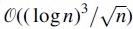for the first-order Markov case. Robin and Schbath (2001) studied the quality of Gaussian approximation by simulations and claimed that the approximation is satisfactory when the expected count exceeds the hundreds. Since the probability of the occurrence of a word is inversely related to the word's length, this claim suggests that the Gaussian approximation would work badly for infrequent words, which are likely to be long words. Therefore, based on previous study, for a k-th order VLMC model with cardinality m of categorical space, the sample of at least $100\times C{m}^k$ (C is a constant) in length is required.

4.4. VLMC-C outperforms VLMC-B in model compression for real genomic sequence data

We investigate the model compression capabilities of VLMC-C and VLMC-B by applying to real genomic sequence data. We first analyze a whole-genome sequence of E. coli containing $4,705,562$ bp using VLMC-B and VLMC-C. VLMC-B constructs a context tree of order 8 containing 2828 contexts, whereas the VLMC-C algorithm reconstructs a context tree of order 7 containing 1334 branches (Fig. 5). Both algorithms greatly decrease the dimensionality of free parameters compared with a full MC model with the same order ($16,384$ branches for a full MC of order 7 and $65,536$ branches for a full MC of order 8). Besides, the number of contexts in the estimated context tree by VLMC-C is merely half of the one obtained by VLMC-B while their orders of the two context trees are almost the same. VLMC-B basically uses contexts with length 6 to model underlying random process, whereas VLMC-C mainly employs the contexts with length 5 and 6 (Tables in Fig. 5).

FIG. 5.

VLMC-C constructs a more sparse context tree than that by VLMC-B on the Escherichia coli genome sequence. (a) The estimated context tree by VLMC-C. (b) The estimated context tree by VLMC-B. The tables below the plots show the numbers of contexts of different lengths by VLMC-C and VLMC-B, respectively.

Bayesian information criterion (BIC) is a widely used measure for model selection. It is defined as $BIC=kln\left(N\right)-2ln\left(\widehat{L}\right)$, where k is the number of parameters in a model, N is the length of sequence, and $\widehat{L}$ is the likelihood of the data under the model. The model yielding a low BIC is preferred as such a model balances model complexity with the likelihood of the sequence. Narlikar et al. (2013) showed the superiority of the model selected by the BIC over other models in biological sequence analyses. Therefore, we use BIC to compare the models from VLMC-C and VLMC-B. The BIC value in results by VLMC-C ($12,678,691$) is smaller than that by VLMC-B ($12,727,306$). We can clearly observe that, although achieving similar maximum orders of VLMC, VLMC-C has better performance on balancing model complexity with the likelihood of the sequence.

We also apply VLMC-C and VLMC-B algorithms to the whole genome of SARS-CoV-2 virus with $29,903$ bp (Wu et al., 2020). VLMC-C reconstructs a more sparse tree than VLMC-B (Fig. 6). We use BIC to measure the goodness-of-fit of the two estimated trees. The BIC value computed based on results by VLMC-C ($80,083.46$) is smaller than that by VLMC-B ($80,642.85$), indicating VLMC-C outperforms VLMC-B in estimation of real VLMC model.

FIG. 6.

The context tree structures of SARS-CoV-2 virus reconstructed by (a) VLMC-C and (b) VLMC-B.

5. DISCUSSION

In this study, we derive the asymptotic distribution for testing statistic used in tree-pruning procedure of context algorithm proposed by Bühlmann and Wyner (1999). We prove theoretically and by simulations that the inferred context tree based on a fixed cutoff threshold from a common chi-square distribution used by VLMC-B (Mächler and Bühlmann, 2004) can be highly biased and error prone. Due to the systematic bias inferred by VLMC-B, increasing sequence length cannot help improve the accuracy of inferred context tree structure of VLMC model. In contrast, our theory of adaptive criterion for tree-pruning procedure improves the performance of accuracy of context tree reconstruction clearly: increasing sequence length does markedly enhance its accuracy in tree reconstruction.

Meanwhile, we control the family-wise errors raised by multiple hypothesis testing in VLMC-C algorithm during the tree-pruning procedure. Since the longer branches in context tree tend to contain more redundant information of lagged states, we consider the length of the testing context when setting the significance level $\alpha$. However, it is worth noting that the hypothesis testing for contexts are structured as a tree, indicating the dependency of these hypothesis testing problems. Therefore, our current setting of the significance level of $\alpha$ as that in Bonferroni correction, which assumes the testing independent, can be inappropriate. Further study for correction of multiple dependent hypothesis testing with organized structures will be considered in future work.

6. APPENDIX

6.1. Equivalence of ${\Delta }_{wu}$ and $\Delta {\prime }_{wu}$

The estimated likelihood function can be factorized into the products of a series of conditional probabilities based on the depending structure corresponding to the context tree. Under hypothesis H₀ and H₁, the decomposed terms are the same except for the terms, which are conditioned on context wu and w, that is, 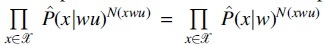holds under H₀ while it does not under H₁. Then, the likelihood ratio test statistic can be simplified and reformulated as follows:

It implies that the two statistics are equivalent except that $\Delta {\prime }_{wu}$ is twice time larger than ${\Delta }_{wu}$.

6.2. Proof of Theorem 1

Theorem 1 mainly follows the studies on asymptotic distribution of differences between overlapping word counts and its estimated expectations (Lundstrom, 1990; Prum et al., 1995; Reinert et al., 2005). We first present the relevant studies in Lemma 1 used in the proof of Theorem 1.

Lemma 1. Consider a sequence of observations of length n from a homogeneous m-th order MC. Given a family of q words $\left\{s^1,s^2,\cdots ,s^q\right\}$, if all the words have the same length l_s and $m=l_s-2$, then

$${\left(\begin{array}{c}\frac{N\left(s^1\right)-Ê\left(s^1\right)}{\sqrt{n}}\\ \cdots \\ \frac{N\left(s^q\right)-Ê\left(s^q\right)}{\sqrt{n}}\\ \end{array}\right)}_{q\times 1}{\to }^{P}N\left(0,{\Sigma }_{q\times q}\right),$$ (8)

where is the maximum likelihood estimator of the expectation of number of overlapping occurrences of word sⁱ. And

where $P\left(s\right)$ denotes the stationary distribution of word s, $s^{-}$ denotes the word after deleting the last letter of word s, ${}^{-}s$ denotes the word after deleting the first letter of s, and ${}^{-}{s}^{-}$ denotes the word after deleting both the first and the last letter of s.

Proof of Theorem 1:

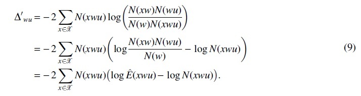
• (i). $Ê\left(xwu\right)=\frac{N\left(xw\right)N\left(wu\right)}{N\left(w\right)}$ is the maximum likelihood estimator of the expectation of the overlapping occurrence number of word xwu in sequence, that is, $E\left(N\left(xwu\right)\right)$, under null hypothesis (Reinert et al., 2005). And by law of large numbers, $Ê\left(xwu\right)∕N\left(xwu\right)\to 1$ holds almost surely under the null hypothesis. Then, Theorem 1 (i) holds directly from Lemma 1.

• (ii). We first substitute $\widehat{P}\left(x|w\right)=\frac{N\left(xw\right)}{N\left(w\right)},\widehat{P}\left(x|wu\right)=\frac{N\left(xwu\right)}{N\left(wu\right)}$ to $\Delta {\prime }_{wu}$, then we have

Using the Taylor expansion, we have

$$\begin{array}{cc}logÊ\left(xwu\right)-logN\left(xwu\right)=& \frac{Ê\left(xwu\right)-N\left(xwu\right)}{N\left(xwu\right)}-\frac{{\left(Ê\left(xwu\right)-N\left(xwu\right)\right)}^2}{2N{\left(xwu\right)}^2}\\ & +O\left({\left(Ê\left(xwu\right)-N\left(xwu\right)\right)}^3\right).\\ \end{array}$$ (10)

Then, $\Delta {\prime }_{wu}$ becomes

In the equation, the first term is zero because

By law of large numbers, $Ê\left(xwu\right)∕N\left(xwu\right)\to 1$ holds almost surely under the null hypothesis, thus $Ê\left(xwu\right)-N\left(xwu\right)\to 0$ holds almost surely. Then, the likelihood ratio test statistic $\Delta {\prime }_{wu}$ can be approximated by

Decompose the covariance matrix in (i) , where $M=P{\Lambda }^{1∕2},\Lambda$ is a diagonal matrix with eigenvalues, and $P^{T}P=I_k$. Let $U=M^{-1}Ñ$, then

$$U\sim N\left(0,I_k\right).$$

Thus, we have

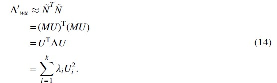
It indicates that $\Delta {\prime }_{wu}$ follows the mixed chi-square distribution, where the weights are the eigenvalues of the covariance matrix ${\tilde{\Sigma }}_{k\times k}$.

6.3. Simulation procedures

For validating our theorem and comparison with VLMC-B algorithm by Mächler and Bühlmann (2004), we simulate a VLMC model of order $k=3$. The initial k letters are set by randomly sampling from the $4^k$ combinations of states in $X=\left\{A,C,G,T\right\}$ with equal probability. Based on the initial k letters, the next letter is generated by searching the context in its lagged k states, followed by sampling according to the transition probabilities in Table 1. Repeating this process, we generate $N=10^5$ letters to form an observational sequence. Under various random seeds of the R software, we have generated a total of $R=3000$ such sequences.

6.4. Significance level setting

In our context algorithm of VLMC-C, to control the type I error rates (focus on family-wise error rate here), the significance level for each test in i-th level of tree is set to be ${\alpha }_i=\frac{{\alpha }_0}{L_i\times K}$, where L_i is the number of candidate leaves to prune once the pruning process is done for the $\left(i+1\right)$-th layer, K is the order of initial context tree ${\widehat{\tau }}_0$, and ${\alpha }_0$ is a given significance level. During the estimation of context tree, the number of nodes to be tested on the i-th layer is denoted as n_i, where $n_i\le L_i$ since not all nodes in i-th layer are leaves. And the number of layers to be tested is denoted as I, where $I\le K$ apparently.

It can be seen with such setting, the probability of making zero type I errors is smaller than ${\alpha }_0$. It follows that

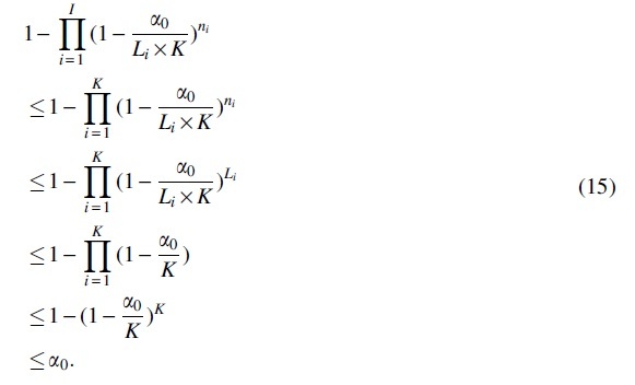
6.5. Pseudocode of VLMC-C algorithm

Algorithm 1: Pseudocode of VLMC-C
Input: Sequence $S=\left\{x_1,x_2,\dots ,x_N\right\}$ generated from finite-state space $X$; significance level ${\alpha }_0$ (${\alpha }_0=0.05$ by default);
THRESHOLD.GEN">valign="bottom"> THRESHOLD.GEN (the default is $max\left(2,round\left(\frac{\sqrt{N}}{\left|X\right|}\right)\right)$);
Output: Context tree $\tau$
Initialize: Build an initial context tree ${\tau }_0$ where each branch corresponds
to a word occurring at least THRESHOLD.GEN. For each branch, set a
label Tested_flag $\leftarrow False$. Denote the order of ${\tau }_0$ by K. Let $\tau \leftarrow {\tau }_0$;
while 1 do
$branches\leftarrow$ the branches of $\tau$ with greatest length and their
corresponding Tested_flag = = False;
if #(branches) = = 0 then
break;
end
$L\leftarrow$ the number of leaves of $\tau$;
$\alpha \leftarrow \frac{{\alpha }_0}{L\times K}$;
for branch in branches do
$ifpruned\leftarrow$ pruning_fun (branch, S, $X$, $\alpha$);
if $ifpruned==True$ then
prune the terminal node of branch, update $\tau$;
else
update the label of branch Tested_flag$\leftarrow$True;
end
end
if all Tested_flag = = True then
break;
end
end
return $\tau$

Algorithm 2: Pseudocode of pruning_fun
Input: Testing branch wu; sequence $S=\left\{x_1,x_2,\dots ,x_N\right\}$; finite state
space $X$; significance level $\alpha$;
Output: Boolean value $ifpruned$
Count $N\left(w\right),N\left(wu\right),N\left(xw\right),N\left(xwu\right)$ and compute $P\left(w\right)$, $P\left(wu\right)$, $P\left(xw\right)$,
$P\left(xwu\right)$;
$E\left(xwu\right)\leftarrow \frac{N\left(xwu\right)}{N\left(xw\right)N\left(wu\right)}$;
$\Delta \leftarrow {\sum }_{x\in X}{\left(N\left(xwu\right)-E\left(xwu\right)\right)}^2∕E\left(xwu\right)$;
Compute covariance $\Sigma$ as
${\Sigma }_{ij}=\sqrt{P\left(x_{i}wu\right)P\left(x_{j}wu\right)}\left(1_{\left\{x_i=x_j\right\}}∕P\left(x_{i}wu\right)-1∕P\left(wu\right)-1_{\left\{x_i=x_j\right\}}∕P\left(x_{i}w\right)+1∕P\left(w\right)\right);$
$\lambda \leftarrow$ eigenvalues of $\Sigma$;
$l\leftarrow 1$;
while $l\le 10^5$ do
$gausssample\leftarrow \left|X\right|$ Gaussian samples;
$chisqsample\leftarrow gausssampl{e}^2$;
$mixchisq\left[l\right]\leftarrow {\sum }_{i=1}^{\left|X\right|}{\lambda }_i\times chisqsample$;
$l\leftarrow l+1$;
end
$quantile\leftarrow$ the $1-\alpha$ quantile of $mixchisq$;
if $\Delta <quantile$ then
$ifpruned\leftarrow$ True;
else
$ifpruned\leftarrow$ False;
end
return if_pruned

AVAILABILITY OF DATA

The whole-genome sequence of Escherichia coli data was downloaded under accession number NZ_CABFNN010000001 with version NZ_CABFNN010000001.1. The whole genome of SARS-CoV-2 virus data was downloaded from GenBank under accession number MN908947. The codes of VLMC-C are available at https://github.com/ShaokunAn/VLMC-C. The VLMC-B was implemented using the R package VLMC (Mächler and Bühlmann, 2004).

AUTHOR DISCLOSURE STATEMENT

The authors declare they have no conflicting financial interests.

FUNDING INFORMATION

L.W. was supported by the National Key Research and Development Program of China under Grant 2019YFA0709501 and the National Natural Science Foundation of China (No. 12071466). F.S. was supported by the National Institutes of Health Grants R01GM120624 and 1R01GM131407 and the National Science Foundation Grant EF-2125142.

REFERENCES

- Arnold, J., Cuticchia, A.J., Newsome, D.A., et al. 1988. Mono-through hexanucleotide composition of the sense strand of yeast DNA: A Markov chain analysis. Nucleic Acids Res. 16, 7145–7158. [DOI] [PMC free article] [PubMed] [Google Scholar]
- Avery, P.J. 1987. The analysis of intron data and their use in the detection of short signals. J. Mol. Evol. 26, 335–340. [DOI] [PubMed] [Google Scholar]
- Billingsley, P. 1961. Statistical Inference for Markov Processes, volume 2. University of Chicago Press, Chicago, IL. [Google Scholar]
- Blaisdell, B.E. 1985. Markov chain analysis finds a significant influence of neighboring bases on the occurrence of a base in eucaryotic nuclear DNA sequences both protein-coding and noncoding. J. Mol. Evol. 21, 278–288. [DOI] [PubMed] [Google Scholar]
- Bühlmann, P. 2000. Model selection for variable length Markov chains and tuning the context algorithm. Ann. Inst. Stat. Math. 52, 287–315. [Google Scholar]
- Bühlmann, P., and Wyner, A.J.. 1999. Variable length Markov chains. Ann. Stat. 27, 480–513. [Google Scholar]
- Dunn, O.J. 1961. Multiple comparisons among means. J. Am. Stat. Assoc. 56, 52–64. [Google Scholar]
- Gentleman, J.F., and Mullin, R.C.. 1989. The distribution of the frequency of occurrence of nucleotide subsequences, based on their overlap capability. Biometrics 45, 35–52. [PubMed] [Google Scholar]
- Hong, J. 1990. Prediction of oligonucleotide frequencies based upon dinucleotide frequencies obtained from the nearest neighbor analysis. Nucleic Acids Res. 18, 1625–1628. [DOI] [PMC free article] [PubMed] [Google Scholar]
- Huang, H. 2002. Error bounds on multivariate normal approximations for word count statistics. Adv. Appl. Probab. 34, 559–586. [Google Scholar]
- Kleffe, J., and Borodovsky, M.. 1992. First and second moment of counts of words in random texts generated by Markov chains. Bioinformatics 8, 433–441. [DOI] [PubMed] [Google Scholar]
- Lundstrom, R. 1990. Stochastic models and statistical methods for DNA sequence data. Ph.D. thesis, University of Utah. [Google Scholar]
- Mächler, M., and Bühlmann, P.. 2004. Variable length Markov chains: Methodology, computing, and software. J. Comput. Graphical Stat. 13, 435–455. [Google Scholar]
- Narlikar, L., Mehta, N., Galande, S., et al. 2013. One size does not fit all: On how Markov model order dictates performance of genomic sequence analyses. Nucleic Acids Res. 41, 1416–1424. [DOI] [PMC free article] [PubMed] [Google Scholar]
- Pevzner, P.A., Borodovsky, M.Y., and Mironov, A.A.. 1989. Linguistics of nucleotide sequences. I: The significance of deviations from mean statistical characteristics and prediction of the frequencies of occurrence of words. J. Biomol. Struct. Dyn. 6, 1013–1026. [DOI] [PubMed] [Google Scholar]
- Prum, B., Rodolphe, F., and De Turckheim, E.. 1995. Finding words with unexpected frequencies in deoxyribonucleic acid sequences. J. R. Stat. Soc. Series. B. Methodol. 57, 205–220. [Google Scholar]
- Reinert, G., Schbath, S., and Waterman, M.S.. 2000. Probabilistic and statistical properties of words: an overview. J. Comput. Biol. 7, 1–46. [DOI] [PubMed] [Google Scholar]
- Reinert, G., Schbath, S., and Waterman, M.S.. 2005. Chapter 6—Statistics on words with applications to biological sequences, 268–352. In Lothaire, M., ed. Applied Combinatorics on Words. Cambridge University Press, New York. [Google Scholar]
- Ren, J., Song, K., Deng, M., et al. 2016. Inference of Markovian properties of molecular sequences from ngs data and applications to comparative genomics. Bioinformatics 32, 993–1000. [DOI] [PMC free article] [PubMed] [Google Scholar]
- Rissanen, J. 1983. A universal data compression system. IEEE Trans. Inf. Theory. 29, 656–664. [Google Scholar]
- Robin, S., and Schbath, S.. 2001. Numerical comparison of several approximations of the word count distribution in random sequences. J. Comput. Biol. 8, 349–359. [DOI] [PubMed] [Google Scholar]
- Wan, L., Kang, X., Ren, J., et al. 2020. Confidence intervals for Markov chain transition probabilities based on next generation sequencing reads data. Quant. Biol. 8, 143–154. [DOI] [PMC free article] [PubMed] [Google Scholar]
- Waterman, M.S. 1995. Introduction to Computational Biology: Maps, Sequences and Genomes. Chapman & Hall/CRC Interdisciplinary Statistics. Taylor & Francis, New York. [Google Scholar]
- Wu, F., Zhao, S., Yu, B., et al. 2020. A new coronavirus associated with human respiratory disease in china. Nature 579, 265–269. [DOI] [PMC free article] [PubMed] [Google Scholar]
Associated Data
This section collects any data citations, data availability statements, or supplementary materials included in this article.
Data Availability Statement