Abstract
In the last few decades, several epidemic diseases have been introduced. In some cases, doctors and medical physicians are facing difficulties in identifying these diseases correctly. A machine can perform some of these identification tasks more accurately than a human if it is trained correctly. With time, the number of medical data is increasing. A machine can analyze this medical data and extract knowledge from this data, which can help doctors and medical physicians. This study proposed a lightweight convolutional neural network (CNN) named ChestX-ray6 that automatically detects pneumonia, COVID19, cardiomegaly, lung opacity, and pleural from digital chest x-ray images. Here multiple databases have been combined, containing 9,514 chest x-ray images of normal and other five diseases. The lightweight ChestX-ray6 model achieved an accuracy of 80% for the detection of six diseases. The ChestX-ray6 model has been saved and used for binary classification of normal and pneumonia patients to reveal the model’s generalization power. The pre-trained ChestX-ray6 model has achieved an accuracy and recall of 97.94% and 98% for binary classification, which outweighs the state-of-the-art (SOTA) models.
Keywords: Convolutional neural network (CNN), ChestX-Ray6, COVID19, Cardiomegaly, DenseNet121, Lung opacity, MobileNetV2, VGG19, Pneumonia, Pleural, ResNet50
1. Introduction
In this era of computing, medical diagnosis can be highly associated with machine learning on an enormous scale. Automation of medical diagnosis is day by day improving to its desired level. X-ray images play a significant role here. X-ray image analysis-based machine learning tools can provide great assistance to radiologists. Machine can detect many fatal diseases by analyzing X-ray images. Pneumonia, COVID19 based pneumonia, lung opacity, pleural, cardiomegaly, and various heart diseases can be detected from X-ray image analysis. Image analysis using a computer can make the diagnosis system faster and cost-effective.
Pneumonia is one kind of lung disease that is caused by viruses, bacteria, or fungi. It is one of the top diseases that causes many deaths every year in developed, developing, and underdeveloped countries. The fatality rate is higher among children. In 2016, 1.2 million children within five years age range were infected by pneumonia, and among them, 880,000 died (Jain, Gupta et al., 2020, Nahiduzzaman, Goni et al., 2021). When a patient is infected by pneumonia, it causes inflammation in the lung’s air sacs, filling them. Because of that, the patient finds it difficult to breathe. If we detect pneumonia timely and start the treatment process, the mortality rate can be lessened. The radiologists use X-ray images to detect pneumonia by looking at the images. The process takes more time as it is checked manually. Also, there are not enough radiologists to speed up the detection process.
COVID19, a disease caused by the novel coronavirus, has created the pandemic of the century. It has reached every corner of the globe and causing thousands of deaths every single day. The whole world is suffering to provide adequate medication to the people. Even the number of newly infected people is so high that there are not enough facilities for testing. Also, infection to death is so short that we do not have enough time to provide not prominent but influential medication. One of the major symptoms of COVID19 is getting pneumonia. Thus, chest X-ray image analysis can improve the testing speed if we correctly detect COVID19 from the image analysis. Also, lung opacity, cardiomegaly, pleural, and many other disease detection can be aided by machine learning to develop an automated and better health care system.
In this paper, we have developed a lightweight deep learning-based model that can detect multiple diseases using chest X-ray analysis. We have used Convolutional Neural Network (CNN) for creating a model named ChestX-ray6. Also, we have used this model as a pre-trained model for binary classification of pneumonia and non-pneumonia and compared the results with other pneumonia detection models to show the generalization capability of the ChestX-Ray6 model. The critical contribution of this research are:
-
•
Several datasets have been combined for more variations and created a multiclass environment.
-
•
A lightweight CNN model named ChestX-Ray6 has been proposed to detect six types of diseases from chest X-ray images.
-
•
Augmentation has been used to balance the datasets, and the model’s performance improved.
-
•
The models’ performance has been compared with different transfer learning approaches, VGG19, ResNet50, DenseNet121, and MobileNetV2, at a new combined dataset in terms of classification criteria, parameters, and processing time.
-
•
The pre-trained ChestX-Ray6 model has been used for binary classification of pneumonia disease with a relatively small dataset. The model surpassed the state-of-art accuracy, precision, and recall.
2. Literature review
Various neural network-based approaches have already been developed for detecting diseases from different types of medical images (Islam et al., 2022, Nahiduzzaman, Islam et al., 2021). Rajpurkar et al. (2017) used deep learning on the ChestX-ray14 dataset and developed a model called CheXNet, which contained 121 layers. They provided a comparison of the results with practicing radiologists, while working with 14 other diseases alongside pneumonia. Guan et al. (2018) developed an AG-CNN model also using ChestX-ray 14 dataset for detecting thorax disease and achieved an average AUC of 0.871. Jain, Nagrath et al. (2020) developed 6 models for detecting pneumonia. Two of these models used 2 and 3 layer-based CNN and could detect pneumonia with 85.26% and 92.3% accuracy. The accuracy of the remaining four models — pre-trained VGG-16, VGG-19, ResNet-50, and Inception-V3 — was 87.28%, 88.46%, 77.56%, and 70.99%, respectively. They also suggested that those transfer learning-based pre-trained models can overcome the vanishing gradient problem. On the Mendeley X-ray image dataset, Chouhan et al. (2020) employed CapsNet, which made use of a group of neurons known as the capsule, to identify pneumonia. They combined convolutions with capsules to develop some models that outperformed the previously proposed models. Using models named Integration of convolutions with capsules (ICC), ensemble of convolutions with capsules (ECC), and EnCC, they achieved 95.33%, 95.90%, and 96.36% accuracy, respectively.
To detect pneumonia, Mittal et al. (2020) employed two basic CNN and multi-layer perceptron deep learning models. They achieved 92.16% and 94.40% accuracy using MLP and CNN, respectively. Ayan and Ünver (2019) used transfer learning models: Xception and VGG-16 for training the X-ray images to detect pneumonia. They found that the VGG-16 approach outperforms the Xception model with 87% accuracy. Sharma et al. (2020) used different deep learning-based approaches for extracting features from X-ray images on the pneumonia dataset. They showed that, data augmentation could improve the performance of the model. Moreover, they also analyzed the impact of using dropout in the models and achieved the highest 90.68% test accuracy with augmentation & dropout, and without augmentation & dropout, the accuracy was 74.98%. Liang and Zheng (2020) developed a system that could recognize pneumonia by combining residual network and dilated convolution. They discovered that dilated convolution minimized information loss for the depth of the deep learning model and the residual network was able to help overcome overfitting. With these techniques, they were able to achieve an f1 score of 92.7%.
Several studies have been performed to detect COVID19 from CT and chest X-ray images (Islam & Nahiduzzaman, 2022). Heidari et al. (2020) used X-ray images to detect COVID19 based pneumonia and developed a convolutional neural network-based model that could detect COVID-19 with 98.8% accuracy. The overall accuracy of the model was 94.0%. Candemir et al. (2018) used X-ray images for the detection of cardiomegaly. Using CNN based ImageNet model, they were able to detect cardiomegaly with 88.24% accuracy. In addition, the CXR-based pre-trained model provided 89.86% accuracy. Maduskar et al. (2016) used segmentation and image localization-based techniques to extract features for supervised learning models and a tuberculosis dataset. They were successful in creating an automated method that could accurately identify pleural effusion. Khan, Sohail, Zahoora and Qureshi (2020) performed a survey on the most recent different architectures of CNN. In this survey, they focused to classify the CNN architectures into seven types of categories based on spatial exploitation, depth, width, attention, etc. Khan, Sohail, Zafar and Khan (2020) proposed two models, namely COVID-RENet-1 and COVID-RENet-2 architectures, for COVID19 specific pneumonia analysis. Furthermore, they employed regional and edge-based operations. Finally, they used a support vector machine algorithm for prediction and achieved an accuracy, precision, F-score, and sensitivity of 98.53%, 98%, 98%, and 99%, respectively. Khan, Sohail, Khan and Lee (2020) developed two-stage CNNs where in the first stage, they enhanced CT images using a two-level discrete wavelet transformation, and then they used a segmentation model for the identification of COVID19. They achieved an accuracy of 98.80% and a recall of 0.99. Khan, Sohail and Khan (2020) proposed a CB-STM-RENet that was trained on three different datasets and compared their work with the existing works while they achieved accuracy and precision of 97% and 93% respectively.
3. Deep network architectures
In this section, we have described different types of deep CNN models which are used to identify multiple diseases using chest X-ray images. First, we have proposed a basic CNN model for predicting these multiple diseases. Then we have used the most advanced models which are ResNet50 (He et al., 2016), DenseNet121 (Huang et al., 2017), VGG19 (Simonyan & Zisserman, 2014), and MobileNetV2 (Sandler et al., 2018). All those models are different in architecture to achieve better performance. CNN was first used by LeCun et al. for recognition of handwritten zip codes in 1989 (LeCun et al., 1989). This network is one kind of deep neural network that is commonly used in the analysis of visual images (Valueva et al., 2020). CNN is also used in processing data, for instance, 1D sequences, 2D images such as medical image analysis and classification, and 3D videos (Jiang et al., 2018, Litjens et al., 2017, Sun et al., 2017). CNN was designed based on the architecture of the biological processes in which the type of connection between neurons is similar to the organization of the animal visual cortex (Fukushima and Miyake, 1982, Hubel and Wiesel, 1968, Matsugu et al., 2003). CNN is one kind of multilayer perceptron (MLP). But, CNN has two main peculiarities, one is local connectivity, and another is shared weights (Albawi et al., 2017). These two peculiarities have two main advantages: one ensures the affine invariance of the networks, and another diminishes the number of parameters. These types of networks are most commonly used to extract knowledge from image data (Xu et al., 2018). For this reason, we have used CNN for multiclass classification from X-ray images. Fig. 1 shows the basic architecture of CNN. It contains an input, an output layer, and between these two layers, multiple hidden layers have resided. The first few stages of hidden layers are consist of a convolutional layer (CL) which convolve with multiplication or dot product.
Fig. 1.
Basic architecture of CNN.
3.1. Convolution layer
The image passes through the CLs in the form of a matrix. CLs are used to extract knowledge or learn features from the input matrix of the image (Bailer et al., 2018). A group of filters, kernels, or feature detectors of various dimensions such as 3 × 3, 5 × 5, etc., are moved on the whole input image. The process means that the filters convolve with the matrix of the image and map a specific matrix which is known as a feature map (Jain, Nagrath et al., 2020). After each convolutional operation, the image dimensions are reduced, making the image easier to process.
3.2. Activation layer
The activation layer is very effective because it helps the CNN to estimate nearly any nonlinear function (Goyal et al., 2019). There are several activation functions, for instance, ReLU, sigmoid, tangent, etc. Most often, ReLU is used as an activation function because it is efficient, faster, remove vanishing gradient problem and gain better performance than any other activation function (Jain, Nagrath et al., 2020, Krizhevsky et al., 2017).
Another activation function is used in the final fully connected layer known as softmax. The process of the softmax includes the probabilistic distribution of the input image to each category where the CNN was learned (Saraiva et al., 2019).
3.3. Pooling layer
The pooling layer is placed between the two successive convolutional layers. Pooling layers reduce the spatial size of the image. Two types of pooling layers are used: one is max-pooling which selects the maximum value, and another is average-pooling which selects the average value from the entire neuron of each cluster at the preceding layer (Ciregan et al., 2012, Mittal, 2020, Yamaguchi et al., 1990). In our model, we used max-pooling with a 2 × 2 filter because it can extract the principal features from the image (Jain, Nagrath et al., 2020). It is used more frequently in real-life application (Krizhevsky et al., 2017, Scherer et al., 2010).
3.4. Fully connected layer
In the fully connected layer, every neuron in one layer is connected to every other neuron in the successive layer. The output of the preceding layer acts as an input of the first fully connected layer. Before feeding these outputs into the fully connected layer, the output of the last layer is flattening the matrix into a vector. Finally, this vector is fed into the fully connected layer. For multi-class classification, the final layer of the CNN uses a softmax as an activation function, which is responsible for making the classification (Hashmi et al., 2020).
3.5. Dropout layer
Almost every parameter is held by a fully connected layer which results in overfitting. There are several methods to reduce overfitting. One of the methods for removing overfitting complexity is dropout (Srivastava et al., 2014). Overfitting is decreased with dropout by randomly avoiding training all neurons of each layer during the training process and hence significantly increase the speed of training (Kovács et al., 2017). Conventionally, a fully connected layer uses dropout. Still, it can be used after the max-pooling layer, followed by the convolution layer.
4. Materials
4.1. Dataset
Most scientists have recently focused on medical images for binary classification using deep learning and transfer learning. In our study, we have focused on the multiclass category using CNN. Here we have merged several medical image datasets to form multiclass. We have collected images of normal and pneumonia patients from the Kaggle chest X-ray pneumonia database with resolutions varying from 400p to 2000p (Mooney, 2018). This chest X-ray images was collected from Guangzhou Women and Children’s Medical Centre, Guangzhou (Jain, Nagrath et al., 2020). Joseph Paul Cohen et al. provided the images of COVID19 patients from which we have collected the samples of COVID19 (Cohen et al., 2020). Images of cardiomegaly, pleural, lung opacity, and no finding patient have been gathered from Neo X-ray database (Ingus, 2019). We have merged images of no-finding patients into images of the normal patient, and then there is a total of 6 classes: normal, pneumonia, COVID19, cardiomegaly, lung opacity, and pleural. Fig. 2 illustrates samples for normal, pneumonia, COVID19, cardiomegaly, lung opacity, and pleural chest X-ray images.
Fig. 2.
Data samples from the dataset, (A) Normal, (B) Pneumonia, (C) COVID19, (D) Cardiomegaly, (E) Lung Opacity, (F) Pleural.
From 9,514 chest X-ray images, the number of normal, pneumonia, COVID19, cardiomegaly, lung opacity, and pleural patients are 2,128, 3,190, 196, 1,000, 1,500, and 1,500.
4.2. Data splitting
The main concept of the deep learning algorithms is that first, we need to learn the model using some of the sample data, for instance, medical image data, and using test data for calculating the model performance (Koza et al., 1996). Using validation data, we can make our model validate, i.e., how accurate the model is. Using this validation set, the model will tune its parameters based on the results (Tyrell et al., 2002).
Finally, the model’s accuracy is calculated by using new unseen samples data known as test data. Using this testing set, the final evaluation of the model has been made. So it is necessary to split the whole medical image data into training, testing, and validation sets. We have used 12% data for testing and 12% data for validating our models. Table 1 shows the details of the training, testing, and validation sets. The dataset contains 7,368 images, 1,144 images for testing, and 1,002 validation sets.
Table 1.
Datasets splitting into training, testing, and validation sets.
| Type | Training set | Testing set | Validation set |
|---|---|---|---|
| Normal | 1,650 | 254 | 224 |
| Pneumonia | 2,471 | 382 | 337 |
| COVID19 | 148 | 28 | 20 |
| Cardiomegaly | 775 | 120 | 105 |
| Lung opacity | 1,162 | 180 | 158 |
| Pleural | 1,162 | 180 | 158 |
| Total | 7,368 | 1,144 | 1,002 |
5. Proposed methodology
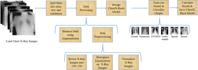
In this article, we have tried to give an optimum solution for predicting multiclass disease from chest X-ray images. First, we have split the total 9,514 images into training, testing, and validation set that we have described in Section 4.2. From Fig. 2, it is clear that the training data is so imbalanced. We have balanced the training data using augmentation, which will describe afterward in this section. Then we have preprocessed our data and built our lightweight ChestX-Ray6 model. After that, we trained our model and calculated our model accuracy using different types of performance measures equations. Fig. 3 shows the block diagram of our proposed methodology for multiclass classification.
Fig. 3.
Proposed methodology for multiclass classification.
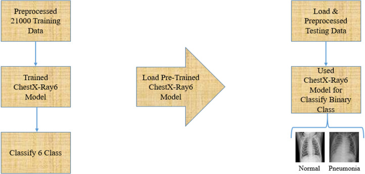
For binary classification, we have followed the concept of transfer learning models. Transfer learning models concentrate on extracting knowledge while solving one problem and using this knowledge to solve another problem (West et al., 2007). In this article, we only test our pre-trained ChestX-ray6 model using various test data from the different datasets and finally classify two classes of normal and pneumonia. Fig. 4 demonstrates the proposed architecture for binary classification.
Fig. 4.
Proposed methodology for binary classification.
5.1. Data balancing
Data balancing is one of the crucial parts of training the model. Because if the dataset is imbalanced, for instance, if the number of images of one class is two or three times more significant than another class, then the performance measures might not be feasible or optimum (Fernández et al., 2008). So it plays a considerable part in balancing the training data. The training data is highly imbalanced because of the number of chest X-ray images for normal, pneumonia, COVID19, cardiomegaly, lung opacity, and the pleural patient is 1,723, 2,583, 158, 810, 1,215, and 1,215 respectively. Hence, we must balance our training data. There are several techniques for balancing the data. In this article, we have balanced training our data using data augmentation. After augmentation, we have 21,000 chest X-ray images and each class has 3,500 ray images.
Again, if we trained our model using a larger dataset, then our model would give better performance because suitable training of CNN claims big data (Rahman et al., 2020). With the help of image augmentation, we made the smaller image datasets large. Besides that, during training, the model data augmentation is used to reduce the overfitting problem and behaves like a regularizer (Albawi et al., 2017, Shorten and Khoshgoftaar, 2019).
In this article, we have used five augmentation methods to create new training sets as demonstrated in Fig. 5. We have used 45° of rotation. We have translated the image in a horizontal direction (width shift) by 20% and in a vertical direction (height shift) by 20% as demonstrated in Fig. 5C, D, respectively. In total, 20% of image shearing and zooming are done as shown in Fig. 5E, F, respectively.
Fig. 5.
(A) Original image, (B) Image after rotation, (C) Image after width shift, (D) Image after height shift, (E) Image after shearing, (F) Image after zooming.
5.2. Data preparation
Data preprocessing is an essential part of CNN because the classification results depend on how well we preprocess our image data. First, we resized the image into a dimension of 150 × 150 pixels for our training process. Then we performed histogram equalization and normalized the resized image, as demonstrated in Fig. 3.
In image processing, histogram equalization is used to adjust or improve the contrast of the image (Hum et al., 2014). This method dramatically impacts the images, which have backgrounds and foregrounds that are both dark or bright. Hence, this method significantly affects images of X-rays, satellites, etc. For that reason, we performed histogram equalization on the chest X-ray images. Then we performed normalization on these processed images.
In image processing, the range of pixel intensity values has changed in the normalization process (Gonzalez & Woods, 2008). In computer vision, every image is represented as a group of pixels, where the pixel value 0 means the color of the pixel is white, and the pixel value 255 indicates the color of the pixel is black. Depending on the magnitude of the pixel value, the color of the images varies from white to dark or dark to white (Chunduri, 2018). So we need a vast number of pixel values to represent our image, which is more complex. To reduce this complexity, we normalized our images by dividing the pixel value by 255, and finally, we reduced the scale from 0–255 to 0–1. Consequently, after normalization, we could represent our image using pixel values ranging from 0 to 1.
5.3. ChestX-Ray6 model
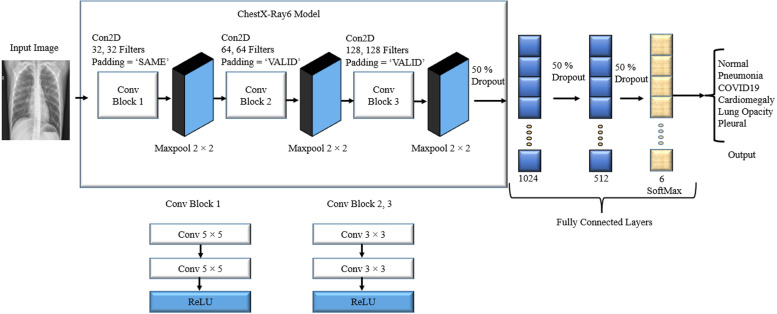
Designing a CNN model is the most critical part of the research. When designing a model, we need to keep in mind that we should build a model that gives the best classification accuracy and reduces both layers and processing time. Moreover, it should also correctly diagnose the disease to help the medical physicians provide the proper treatment for the patient. We have used the convolution layer to extract the relevant features from the chest X-ray images that significantly impacted the diseases and passed those features through the fully connected layer to correctly diagnose the condition. Fig. 6 reveals our proposed lightweight CNN model named ChestX-Ray6 for classifying six classes of disease.
Fig. 6.
Proposed lightweight ChestX-Ray6 model for multiclass classification.
Since we proposed a lightweight CNN model, as a result, six convolutional layers and two dense layers have been used. ReLU has been used as an activation function after every two convolutional layers. A 2 × 2 max pool has been used after each convolutional block. For more reduction in complexity, three dropouts have been used: one dropout has been used after the final convolutional layer and two after each dense layer. The result has been determined by applying the filters to all image tuples; hence, we have inserted the ‘SAME’ padding in the first two convolution layers. Due to this, border elements have been investigated because they frequently include critical properties for this particular dataset. Padding has been omitted from the border elements during the design process. The padding designated as ‘VALID’ in the remaining convolutional layers has been used and does not consider the boundary components. Finally, a flattening layer has been used to flatten the matrix into a vector. Then this output is fed into the fully connected layer. A dropout with a 0.5 probability has been used in the first two fully connected layers. This dropout speeds up the processing time of the model and also reduces its overfitting. A softmax activation function has been used to make a prediction in the final fully connected layer. Finally, the cost has been calculated using the sparse categorical cross-entropy cost function depending on the prediction. In addition, the cost function has been determined using back-propagation and features map to make the CNN optimized. In this study, the Adam optimizer has been used because it is very efficient for CNN. Moreover, it also gives better results while training on huge datasets and reduces the computational cost (Kingma & Ba, 2014). The learning rate has been set to 0.001. We have trained the ChestX-Ray6 model using a batch size of 128 and the total number of epochs is 100.
In our ChestX-Ray6 model, the image shape after the first two convolution layers is 150 × 150x32. Afterward, the image shape is 75 × 75x32 after applying the first max-pooling layer. Table 2 shows the rest of the output image shapes and a summary of our ChestX-Ray6 model.
Table 2.
Summary of ChestX-Ray6 model.
| Layer(type) | Output shape | Number of parameters |
|---|---|---|
| Conv1_1(Conv2D) | (None, 150, 150, 32) | 832 |
| Conv1_2(Conv2D) | (None, 150, 150, 32) | 25 632 |
| pool1(MaxPooling2D) | (None, 75, 75, 32) | 0 |
| Conv2_1(Conv2D) | (None, 73, 73, 64) | 18 496 |
| Conv2_2(Conv2D) | (None, 71, 71, 32) | 36 928 |
| pool2(MaxPooling2D) | (None, 35, 35, 64) | 0 |
| Conv3_1(Conv2D) | (None, 33, 33, 128) | 73 856 |
| Conv3_2(Conv2D) | (None, 31, 31, 128) | 147 584 |
| pool3(MaxPooling2D) | (None, 15, 15, 128) | 0 |
| dropout1(Dropout) | (None, 15, 15, 128) | 0 |
| flatten(Flatten) | (None, 28800) | 0 |
| fc1(Dense) | (None, 1024) | 29 492 224 |
| dropout2(Dropout) | (None, 1024) | 0 |
| fc2(Dense) | (None, 512) | 524 800 |
| dropout3(Dropout) | (None, 512) | 0 |
| fc3(Dense) | (None, 6) | 3 078 |
5.4. Performance matrix for classification
The following performance matrices have been used to compare the results in this study: accuracy, precision, recall, f1-score, and the area under the curve. After our ChestX-Ray6 model had finished training, we calculated its performance for the testing dataset (AUC). One model can achieve high accuracy when the model has high precision and trueness (Menditto et al., 2007) and the accuracy is given by Eq. (1). Precision can be defined as the fraction of related samples among the recovered samples, and the precision is provided by Eq. (2) (Olson & Delen, 2008). Whereas recall could be defined as the fraction of the total number of related samples which are exactly recovered, and the recall is given by Eq. (3) (Olson & Delen, 2008). The F-measure could be defined as the measure of a harmonic mean, and this measure is given by Eq. (4) (Powers, 2020).
| (1) |
| (2) |
| (3) |
| (4) |
In the above equation, for binary classification, true positive (TP) means that pneumonia patient is detected as pneumonia, true negative (TN) means that a normal patient is detected as normal, false positive (FP) means that a normal patient is incorrectly detected as pneumonia. A false-negative (FN) means that the pneumonia patient was incorrectly detected as a normal patient. For multiclass classification, TP means that pneumonia, COVID19, cardiomegaly, lung opacity, and pleural patients are correctly detected as pneumonia, COVID19, cardiomegaly, lung opacity, and pleural, respectively. TN means that a normal patient is detected as normal, FP implies that a normal patient is incorrectly detected as pneumonia or any other four diseases, and FN means that pneumonia or any other four conditions is incorrectly detected as a normal patient.
6. Experimental results and performance analysis
In this section, the experiments and results of different performance measures are presented. We used the Pycharm Community Edition (2020.2.3 × 64) software and Keras with TensorFlow as the backend. We utilized a computer with an Intel(R) Core(TM) i7-6700 CPU @3.40 GHz processor and 32 GB RAM, a NVIDIA GeForce GTX 1650 SUPER 4 GB GPU on a 64-bit Windows 10 Pro operating system for performing the training and testing of our model.
6.1. Performance of the proposed model multiclass classification
We have trained our lightweight ChestX-Ray6 model using 21,000 training data and validated our model using a 1,002 validation set where the number of normal, pneumonia, COVID19, cardiomegaly, lung opacity, and pleural patient images are 224, 337, 20, 105, 158, and 158, respectively. Finally, we have tested our model using the 1,144 test dataset where the number of normal pneumonia, COVID19, cardiomegaly, lung opacity, and pleural patient images are 254, 382, 28, 120, 180, and 180, respectively, for classifying these six classes. We trained our model for 100 epochs, and the batch size is 128. The best training and validation accuracy of our model is 98.56% and 77.34%, respectively. The minimum training and validation losses of our model are 0.09 and 0.58, respectively.
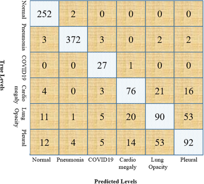
Furthermore, the robustness of our model has been examined by calculating the accuracy, precision, recall, f1-score, and AUC of our model. We have used a confusion matrix for calculating the above measurement, which is demonstrated in Fig. 7. We have also calculated the true positive, true negative, false positive, and false negative using this confusion matrix, which helped us to find our model’s efficiency. For medical data, recall should be maximized because the patient with the disease must be correctly identified. The average precision, recall, and f1-score of our model without augmentation are 66%, 67%, and 66%, respectively, which are shown in Table 3.
Fig. 7.
Confusion matrix for multiclass classification.
Table 3.
Values of performance measures of ChestX-Ray6 model without augmentation.
| Type | Precision | Recall | F1-score |
|---|---|---|---|
| Normal | 74% | 98% | 84% |
| Pneumonia | 96% | 95% | 95% |
| COVID19 | 57% | 61% | 59% |
| Cardiomegaly | 62% | 57% | 60% |
| Lung opacity | 53% | 37% | 44% |
| Pleural | 57% | 52% | 54% |
| Average | 66% | 67% | 66% |
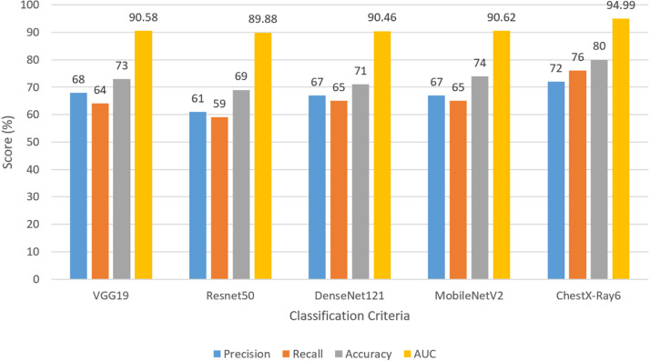
Without augmentation, the area under the curve (AUC) of our model is 92.04% and the overall accuracy of our ChestX-Ray6 model is 75%. The performance of our model has been enhanced using the augmentation technique. Our model’s average precision, recall, and f1-score with augmentation are 72%, 76%, and 73%, respectively. From Table 4 it is observed that the overall performance of the ChestX-Ray6 model is better than the transfer learning model. The accuracy of VGG19, ResNet50, DenseNet121, and MobileNetV2 are 0.73, 0.69, 0.77, and 0.74 respectively. We have achieved better accuracy using our model, which is 0.80.
Table 4.
Values of performance measures of different models with augmentation.
| Type | Precision |
Recall |
||||||||
|---|---|---|---|---|---|---|---|---|---|---|
| ChestX-Ray6 | VGG | ResNet | DenseNet | MobileNet | ChestX-Ray6 | VGG | ResNet | DenseNet | MobileNet | |
| Normal | 0.89 | 0.73 | 0.64 | 0.69 | 0.76 | 0.99 | 0.95 | 0.95 | 0.94 | 0.95 |
| Pneumonia | 0.98 | 0.97 | 0.95 | 0.94 | 0.98 | 0.97 | 0.96 | 0.91 | 0.91 | 0.95 |
| COVID19 | 0.63 | 0.79 | 0.58 | 0.8 | 0.74 | 0.96 | 0.54 | 0.5 | 0.71 | 0.61 |
| Cardiomegaly | 0.68 | 0.62 | 0.56 | 0.52 | 0.59 | 0.63 | 0.59 | 0.45 | 0.6 | 0.5 |
| Lung Opacity | 0.54 | 0.47 | 0.45 | 0.48 | 0.45 | 0.50 | 0.39 | 0.51 | 0.41 | 0.39 |
| Pleural | 0.56 | 0.5 | 0.5 | 0.58 | 0.52 | 0.51 | 0.43 | 0.22 | 0.36 | 0.49 |
| Average | 0.72 | 0.68 | 0.61 | 0.67 | 0.67 | 0.76 | 0.64 | 0.59 | 0.65 | 0.65 |
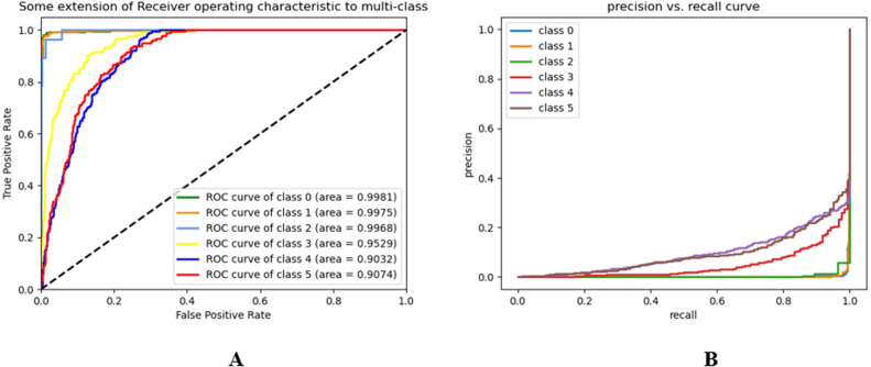
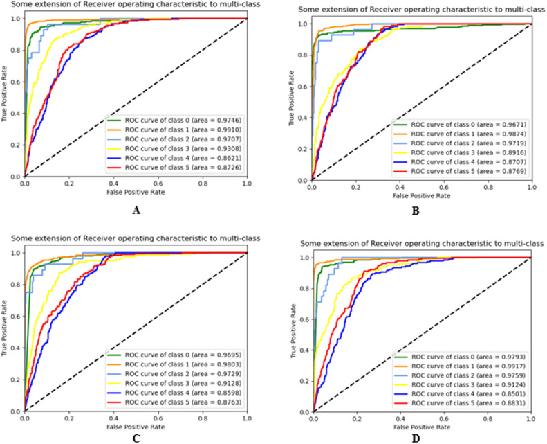
The receiver-operating characteristics (ROC) and precision–recall (PR) curves of our model and different transfer learning algorithms for different classes are demonstrated in Fig. 8, Fig. 9, respectively.
Fig. 8.
(A) ROC, and (B) PR curve of ChestX-Ray6 model.
Fig. 9.
ROC of (A) VGG19, (B) ResNet50, (C) DenseNet121, and (D) MobileNetV2.
The AUC of VGG19, ResNet50, DenseNet121, and MobileNetV2 are 90.58%, 89.88%, 90.46%, and 90.62% respectively. The AUC of our model is 94.99%. From Fig. 10, we have concluded that the overall classification performance of our model is better than other transfer learning models.
Fig. 10.
Graphical comparison for multi-class classification with different approaches.
A lightweight model has been developed here, for that reason, we have measured the layers and processing time to validate the model’s high-speed capability and compared them with the other transfer learning models. The convolutional layers for ChestX-Ra6, VGG19, ResNet50, DenseNet-121, and MobileNetV2 are 6, 16, 50, 121, and 53, respectively, and the training times are 6150.62, 8215.94, 7018.10, 7571.84, and 6457.20 s, respectively. These results could be changed with a different computer’s configuration. The testing time of the ChestX-Ray6 model is 2.72 s, which is quite low compared to other transfer learning models. From the Table 5, it can be concluded that the convolutional layers and processing time of the proposed model are quite less than the other four transfer learning models, which reveals the robustness of the proposed model. From the above discussion, it is understood that the proposed lightweight ChestX-Ray6 performs well in the case of classification criteria and also performs well in terms of architectural complexity and processing time for the detection of six classes from the chest X-ray images. Though the model performed well in the combined dataset, the performance may vary if applied to other datasets. This criterion is not considered in this study.
Table 5.
Convolutional layers and processing time comparison for ChestX-Ray6 with different transfer learning approaches.
| Model | Layers | Train time (s) | Test time (s) |
|---|---|---|---|
| VGG19 | 16 | 8215.94 | 8.17 |
| ResNet50 | 50 | 7018.10 | 5.29 |
| DenseNet121 | 121 | 7571.84 | 9.59 |
| MobileNetV2 | 53 | 6457.20 | 4.03 |
| ChestX-Ray6 | 6 | 6150.62 | 2.72 |
6.2. Visualization analysis
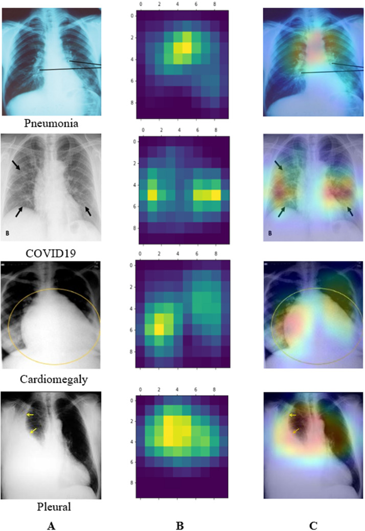
In this section, we have used Grad-CAM (Gradient-weighted Class Activation Mapping) to get a heat map of where pneumonia is most likely to manifest itself (Selvaraju et al., 2017). This technique employs the gradient of a target notion to produce “visual explanations” for CNN models. We have generated a crude localization map using Grad-CAM, showing us where we need to focus on our prediction-conception image. While classifying the six classes, the gradients of the final convolutional layer emphasize the chest X-ray accurately recognized by the filters and represented in the feature maps. The Grad-CAM visualization of the different classes has been shown in Fig. 11. From the visualization, it is observed that the lightweight ChestX-Ray6 model correctly detects the affected region of various lung-related diseases.
Fig. 11.
Gradient-weighted class activation mapping of some diseases using ChestX-Ray6, (A) Original images indicated infected regions by radiologists, (B) Heat map, (C) Grad-CAM.
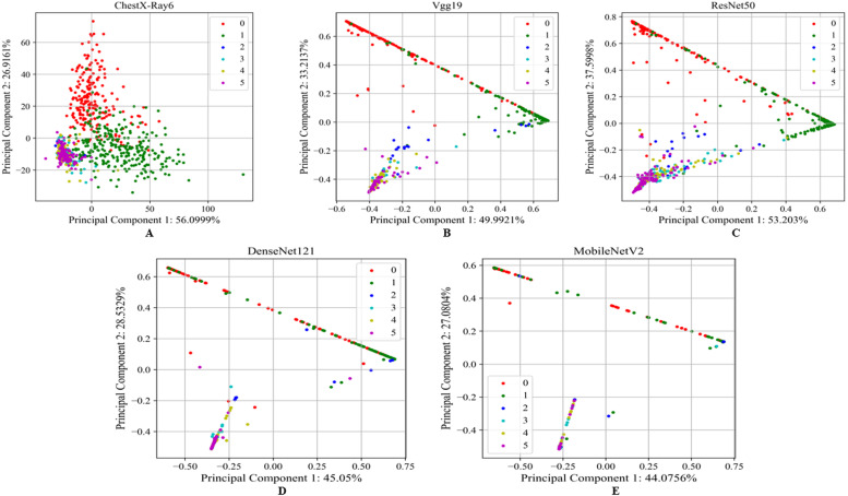
We demonstrated how our proposed model extracted the most discriminant features from the chest X-ray images and visualized them using principal component analysis (PCA). The dimension of the extracted features from the images is too high, and we need to reduce the dimension using PCA for visualization since it is used to convert the higher-dimensional data into a much smaller dimension (Fontes & Soneson, 2011). Our proposed model’s visual discrimination feature space is shown in Fig. 12 through a PCA-based comparison. ChextX-ray6, VGG19, ResNet50, DenseNet121, and MobileNetV2 for the test dataset are shown in Fig. 12 as two-dimensional plots with the first principal component, second principal component and their relative variance. It is observed that the proposed lightweight ChestX-Ray6 model captured more prominent information than the other transfer learning models.
Fig. 12.
PCA based visualization of (A) the proposed lightweight ChextX-ray6 model, (B) VGG19, (C) ResNet50, (D) DenseNet121, and (E) MobileNetV2 for test data.
6.3. Performance of the proposed model for binary classification
In this study, we trained and tested our lightweight ChestX-Ray6 model using a merged dataset with six classes: normal, pneumonia, COVID19, cardiomegaly, lung opacity, and pleural. In this section, we did not train our model but only tested our pre-trained ChestX-Ray6 model using a binary class normal and pneumonia dataset. We have tested our model using multiple folds of the test dataset to calculate our model efficiency and compared the result of our model with other research work to ensure that our ChestX-Ray6 model correctly predicted the diseases better than the other models.
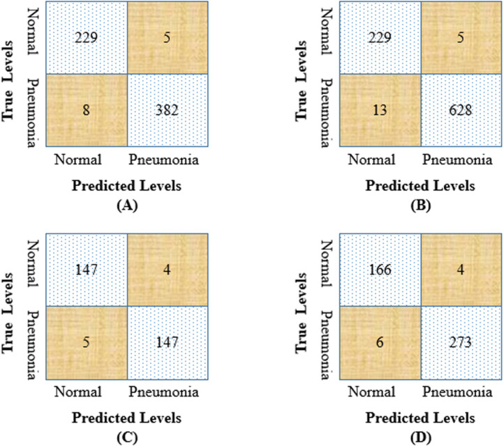
We have tested our model using multiple folds of test data, including 624 (normal: 234, pneumonia: 390), 875 (normal: 234, pneumonia: 641), 303 (normal: 151, pneumonia: 152), and 449 (normal: 170, pneumonia: 279) images of normal and pneumonia patients for comparison with other works.
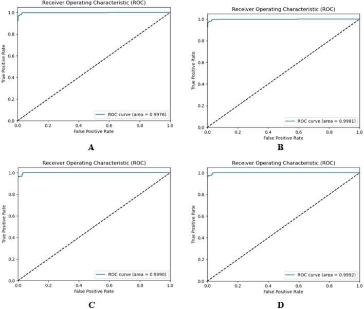
Fig. 13 shows the four ROC curves (also known as AUROC (area under the receiver operating characteristics)) of our pre-trained ChestX-Ray6 model for multiple fold test data. This acts as a significant evaluation metric to estimate the performance of any classification model.
Fig. 13.
ROC curves for binary classification, (A) 624 test images, (B) 875 test images, (C) 303 test images, (D) 449 test images.
Fig. 14 shows the confusion matrix of our pre-trained model for these four-fold test data. From the confusion matrix, we have calculated the precision, recall, f1-score, AUC, and accuracy of our model to test our pre-trained model’s robustness for binary classification. The accuracy of 624, 875, 303, and 449 chest X-ray images are 97.91%, 97.94%, 97.02%, and 97.77% respectively. Table 6 shows the overall values of performance measures for multiple-fold test data.
Fig. 14.
Confusion matrix for binary classification (A) 624 test images, (B) 875 test images, (C) 303 test images, (D) 449 test images.
Table 6.
Values of performance measures of ChestX-Ray6 model for binary classification.
| Test images | Type | Recall | F1-score | AUC | Accuracy |
|---|---|---|---|---|---|
| 624 | Normal | 98% | 97% | – | – |
| Pneumonia | 98% | 98% | – | – | |
| Average | 98% | 98% | 99.76% | 97.91% | |
| 875 | Normal | 98% | 96% | – | – |
| Pneumonia | 98% | 99% | – | – | |
| Average | 98% | 97% | 99.81% | 97.94% | |
| 303 | Normal | 97% | 97% | – | – |
| Pneumonia | 998% | 97% | – | – | |
| Average | 97% | 97% | 99.90% | 97.02% | |
| 449 | Normal | 98% | 97% | – | – |
| Pneumonia | 98% | 98% | – | – | |
| Average | 98% | 98% | 99.92% | 97.77% | |
6.4. Performance comparison with related works
In this section, we have compared our model performance with other existing methods for the same dataset. The lightweight ChestX-Ray6 has been saved and is further used as a transfer learning model. The pre-trained model has been tested on different datasets to detect pneumonia patients, and the result has been compared with the existing work. The details of the existing techniques were described in Section 2. Jain, Nagrath et al. (2020) used two CNN models and some of the transfer learning algorithms (VGG16, VGG19, ResNet50, and Inception-v3) were used to detect the two classes, normal and pneumonia. They used the Kaggle chest X-ray dataset to train their various models and tested them using 624 (normal: 234, pneumonia: 390) images. The best recall and accuracy of their model were 98% and 92.32%, respectively. Chouhan et al. (2020) used Guangzhou Women and Children’s Medical Center dataset for training their ensemble model achieved an accuracy of 96.39%, recall of 99.62%, and an AUC of 99.34%. Ayan and Ünver (2019) achieved good accuracy while using VGG16 over the Xception network. They used the same fold images for testing their model, and the recall and accuracy of their model were 88%, and 87% respectively. Liang and Zheng (2020) used CNN to detect the pneumonia patient. They trained their model using the same dataset and achieved an accuracy of 90.5%, recall of 96.7%, and an AUC of 95.3%. We have tested our pre-trained ChestX-Ray6 model using the same test images and achieved more optimistic results than the existing methods. The precision, recall, f1-score, AUC, and accuracy of our model are 98%, 98%, 98%, 99.76%, and 92.92% respectively which are shown in Table 7.
Table 7.
Performance comparison of ChestX-Ray6 model for binary classification with existing models.
| No of test images | Model | Precision | Recall | F1-score | AUC | Accuracy |
|---|---|---|---|---|---|---|
| 624 | Jain, Nagrath et al. (2020) | – | 98% | 94% | – | 92.31% |
| Chouhan et al. (2020) | 93.28% | 99.62% | – | 99.34% | 96.39% | |
| Ayan and Ünver (2019) | 87% | 88% | 87% | – | 87% | |
| Liang and Zheng (2020) | 89.10% | 96.7% | 92.7% | 95.3% | 90.5% | |
| Proposed Method | 98% | 98% | 98% | 99.76% | 97.92% | |
| 875 | Mittal et al. (2020) | 96.77% | 98.28% | 97.54% | – | 96.36% |
| Proposed Model | 98.43% | 98.28% | 98.59% | 99.81% | 97.94% | |
| 449 | Sharma et al. (2020) | – | – | – | – | 90.68% |
| Proposed Model | 98% | 98% | 98% | 99.92% | 97.77% | |
Mittal et al. (2020) trained their integration of convolutions with capsules (ICC) and an ensemble of convolutions with capsules (ECC) using the Mendeley dataset. They tested their models using 875 (normal:234, pneumonia: 641) test images and achieved the best accuracy with the E4CC model. We have calculated the precision, recall, and f1-score from their confusion matrix. They reached an accuracy of 96.36%, a recall of 98.28%. We have tested our pre-trained ChestX-Ray6 model using the same 875 test images and achieved a better result than the E4CC model. We have achieved an accuracy of 97.94%, a recall of 98.28%, and an AUC of 99.81%.
Sharma et al. (2020) trained their CNN model using the Kaggle chest X-ray dataset. They tested their model using 449 (normal:170, pneumonia:279) test images and achieved an accuracy of 90.68%. We have tested our pre-trained model using the same 449 test images and achieved a higher accuracy of 97.77% than their model. The recall and AUC of our model are 98% and 99.92%, respectively. From the above discussion, it is concluded that the pre-trained ChestX-Ray6 model outperformed six state-of-the-art models for binary classification and validated the robustness of the proposed model.
6.5. Discussion
This section discusses the lightweight ChestX-Ray6 model’s convenience of use to diagnose diseases from a merged dataset.
In this study, a lightweight CNN model has been proposed to classify multiple diseases from chest X-ray images and its performances have been compared with other transfer learning models. The performance is shown in the Table 4. Though the model is simple in architecture, it has only six convolutional layers and two dense layers. Still, the model classification performance is better than the other four models. One of the main concerns of this study is designing a model that provides higher classification accuracy and reduces the number of layers and processing time for large amounts of data. For that reason, here, a lightweight ChestX-Ray6 model has been designed to measure whether it performed well for these criteria in the case of a multiclass environment. Table 5 shows that the convolutional layers and processing time are also less than the other transfer learning models. So, it is concluded that the ChestX-Ray6 model achieved optimistic classification performance results and also reduced layers and processing time.
Another concern of this study is to check the generalization power of the proposed ChestX-Ray6 model. For that reason, the model has been used as a pre-trained model and then measured the classification performance in the case of binary classification. It is observed from the comparison section that the pre-trained model has outperformed various well-known state-of-the-art models. The proposed model achieved a high classification performance for both multiclass and binary classification. Moreover, reduced processing time has made our model a strong candidate for use in real-time applications. These are the main contributions of this study.
7. Conclusion and future work
This work presents a novel lightweight CNN ChestX-Ray6 model for detecting multiple diseases from digital chest X-ray images. We have combined six classes to develop a complex multiclass environment for lung diseases. Hence, the model has more discriminant features to differentiate the classes. Further, classes are balanced using augmentation and preprocessed using various preprocessing techniques such as image normalization and histogram equalization. We trained our model using 21,000 chest X-ray images and saved our model for calculating the performance of our model for binary classification. The classification accuracy for six classes is 80%. Here we have used our ChestX-Ray6 model as a transfer learning model. Hence we tested our pre-trained ChestX-Ray6 model for binary classification of normal and pneumonia patients and achieved an accuracy of 97.94% with precision, recall, and f1-score of 98%, which shows better performance than the previous works. We have also compared different transfer learning algorithms with our ChestX-Ray6 model in other performance criteria. Here, our ChestX-Ray6 model has achieved an excellent performance for both multiclass and binary classification, which can help medical physicians diagnose these types of diseases correctly. We intend to use big data in the future and expand the multiclass to more classes.
CRediT authorship contribution statement
Md. Nahiduzzaman: Conceptualization, Data curation, Formal analysis, Writing – review & editing, Methodology, Project administration. Md. Rabiul Islam: Writing – review & editing, Manuscript editing, Supervision, Validation. Rakibul Hassan: Conceptualization, Writing – review & editing, Writing – original draft, Manuscript editing, Validation.
Declaration of Competing Interest
The authors declare that they have no known competing financial interests or personal relationships that could have appeared to influence the work reported in this paper.
Footnotes
The code (and data) in this article has been certified as Reproducible by Code Ocean: (https://codeocean.com/). More information on the Reproducibility Badge Initiative is available at https://www.elsevier.com/physical-sciences-and-engineering/computer-science/journals.
Data availability
Data will be made available on request.
References
- Albawi S., Mohammed T.A., Al-Zawi S. 2017 International conference on engineering and technology. IEEE; 2017. Understanding of a convolutional neural network; pp. 1–6. [Google Scholar]
- Ayan E., Ünver H.M. 2019 Scientific meeting on electrical-electronics & biomedical engineering and computer science. IEEE; 2019. Diagnosis of pneumonia from chest X-Ray images using deep learning; pp. 1–5. [Google Scholar]
- Bailer C., Habtegebrial T., Stricker D. 2018. Fast feature extraction with CNNs with pooling layers. arXiv preprint arXiv:1805.03096. [Google Scholar]
- Candemir S., Rajaraman S., Thoma G., Antani S. 2018 IEEE Life sciences conference. IEEE; 2018. Deep learning for grading cardiomegaly severity in chest X-rays: an investigation; pp. 109–113. [Google Scholar]
- Chouhan V., Singh S.K., Khamparia A., Gupta D., Tiwari P., Moreira C., Damaševičius R., De Albuquerque V.H.C. A novel transfer learning based approach for pneumonia detection in chest X-ray images. Applied Sciences. 2020;10(2):559. [Google Scholar]
- Chunduri V. 2018. FNORMALIZATION in machine learning AND deep learning. Online URL https://medium.com/transparent-deep-learning/normalization-in-machine-learning-and-deep-learning-56eb33eb0165 (Accessed 20 November 2020) [Google Scholar]
- Ciregan D., Meier U., Schmidhuber J. 2012 IEEE Conference on computer vision and pattern recognition. IEEE; 2012. Multi-column deep neural networks for image classification; pp. 3642–3649. [Google Scholar]
- Cohen J.P., Morrison P., Dao L. 2020. COVID-19 image data collection. arXiv 2003.11597 URL https://github.com/ieee8023/covid-chestxray-dataset. [Google Scholar]
- Fernández A., García S., del Jesus M.J., Herrera F. A study of the behaviour of linguistic fuzzy rule based classification systems in the framework of imbalanced data-sets. Fuzzy Sets and Systems. 2008;159(18):2378–2398. [Google Scholar]
- Fontes M., Soneson C. The projection score-an evaluation criterion for variable subset selection in PCA visualization. BMC Bioinformatics. 2011;12(1):1–17. doi: 10.1186/1471-2105-12-307. [DOI] [PMC free article] [PubMed] [Google Scholar]
- Fukushima K., Miyake S. Competition and cooperation in neural nets. Springer; 1982. Neocognitron: A self-organizing neural network model for a mechanism of visual pattern recognition; pp. 267–285. [Google Scholar]
- Gonzalez R., Woods R. Pearson/Prentice Hall; 2008. Digital image processing. URL https://books.google.com.bd/books?id=8uGOnjRGEzoC. [Google Scholar]
- Goyal M., Goyal R., Lall B. 2019. Learning activation functions: A new paradigm of understanding neural networks. arXiv preprint arXiv:1906.09529. [Google Scholar]
- Guan Q., Huang Y., Zhong Z., Zheng Z., Zheng L. 2018. Diagnose like a radiologist: Attention guided convolutional neural network for thorax disease classification. arXiv preprint arXiv:1801.09927. [Google Scholar]
- Hashmi M.F., Katiyar S., Keskar A.G., Bokde N.D., Geem Z.W. Efficient pneumonia detection in chest xray images using deep transfer learning. Diagnostics. 2020;10(6):417. doi: 10.3390/diagnostics10060417. [DOI] [PMC free article] [PubMed] [Google Scholar]
- He, K., Zhang, X., Ren, S., & Sun, J. (2016). Deep residual learning for image recognition. In Proceedings of the IEEE Conference on computer vision and pattern recognition (pp. 770–778).
- Heidari M., Mirniaharikandehei S., Khuzani A.Z., Danala G., Qiu Y., Zheng B. Improving the performance of CNN to predict the likelihood of COVID-19 using chest X-ray images with preprocessing algorithms. International Journal of Medical Informatics. 2020;144 doi: 10.1016/j.ijmedinf.2020.104284. [DOI] [PMC free article] [PubMed] [Google Scholar]
- Huang, G., Liu, Z., Van Der Maaten, L., & Weinberger, K. Q. (2017). Densely connected convolutional networks. In Proceedings of the IEEE Conference on computer vision and pattern recognition (pp. 4700–4708).
- Hubel D.H., Wiesel T.N. Receptive fields and functional architecture of monkey striate cortex. The Journal of Physiology. 1968;195(1):215–243. doi: 10.1113/jphysiol.1968.sp008455. [DOI] [PMC free article] [PubMed] [Google Scholar]
- Hum Y.C., Lai K.W., Mohamad Salim M.I. Multiobjectives bihistogram equalization for image contrast enhancement. Complexity. 2014;20(2):22–36. [Google Scholar]
- Ingus T. 2019. Neo xrays. Online https://www.kaggle.com/ingusterbets/neo-xrays. (Accessed 19 November 2020) [Google Scholar]
- Islam M.R., Nahiduzzaman M. Complex features extraction with deep learning model for the detection of COVID19 from CT scan images using ensemble based machine learning approach. Expert Systems with Applications. 2022;195 doi: 10.1016/j.eswa.2022.116554. [DOI] [PMC free article] [PubMed] [Google Scholar]
- Islam M.R., Nahiduzzaman M., Goni M.O.F., Sayeed A., Anower M.S., Ahsan M., Haider J. Explainable transformer-based deep learning model for the detection of malaria parasites from blood cell images. Sensors. 2022;22(12):4358. doi: 10.3390/s22124358. [DOI] [PMC free article] [PubMed] [Google Scholar]
- Jain R., Gupta M., Taneja S., Hemanth D.J. Deep learning based detection and analysis of COVID-19 on chest X-ray images. Applied Intelligence: The International Journal of Artificial Intelligence, Neural Networks, and Complex Problem-Solving Technologies. 2020:1–11. [Google Scholar]
- Jain R., Nagrath P., Kataria G., Kaushik V.S., Hemanth D.J. Pneumonia detection in chest X-ray images using convolutional neural networks and transfer learning. Measurement. 2020;165 [Google Scholar]
- Jiang Y.-G., Wu Z., Tang J., Li Z., Xue X., Chang S.-F. Modeling multimodal clues in a hybrid deep learning framework for video classification. IEEE Transactions on Multimedia. 2018;20(11):3137–3147. [Google Scholar]
- Khan S.H., Sohail A., Khan A. 2020. COVID-19 detection in chest X-Ray images using a new channel boosted CNN. arXiv preprint arXiv:2012.05073. [DOI] [PMC free article] [PubMed] [Google Scholar]
- Khan S.H., Sohail A., Khan A., Lee Y.S. 2020. Classification and region analysis of COVID-19 infection using lung CT images and deep convolutional neural networks. arXiv preprint arXiv:2009.08864. [Google Scholar]
- Khan S.H., Sohail A., Zafar M.M., Khan A. 2020. Coronavirus disease analysis using chest X-ray images and a novel deep convolutional neural network. [DOI] [PMC free article] [PubMed] [Google Scholar]
- Khan A., Sohail A., Zahoora U., Qureshi A.S. A survey of the recent architectures of deep convolutional neural networks. Artificial Intelligence Review. 2020;53(8):5455–5516. [Google Scholar]
- Kingma D.P., Ba J. 2014. Adam: A method for stochastic optimization. arXiv preprint arXiv:1412.6980. [Google Scholar]
- Kovács G., Tóth L., Van Compernolle D., Ganapathy S. Increasing the robustness of CNN acoustic models using autoregressive moving average spectrogram features and channel dropout. Pattern Recognition Letters. 2017;100:44–50. [Google Scholar]
- Koza J.R., Bennett F.H., Andre D., Keane M.A. Artificial intelligence in design’96. Springer; 1996. Automated design of both the topology and sizing of analog electrical circuits using genetic programming; pp. 151–170. [Google Scholar]
- Krizhevsky A., Sutskever I., Hinton G.E. Imagenet classification with deep convolutional neural networks. Communications of the ACM. 2017;60(6):84–90. [Google Scholar]
- LeCun Y., Boser B., Denker J.S., Henderson D., Howard R.E., Hubbard W., Jackel L.D. Backpropagation applied to handwritten zip code recognition. Neural Computation. 1989;1(4):541–551. [Google Scholar]
- Liang G., Zheng L. A transfer learning method with deep residual network for pediatric pneumonia diagnosis. Computer Methods and Programs in Biomedicine. 2020;187 doi: 10.1016/j.cmpb.2019.06.023. [DOI] [PubMed] [Google Scholar]
- Litjens G., Kooi T., Bejnordi B.E., Setio A.A.A., Ciompi F., Ghafoorian M., Van Der Laak J.A., Van Ginneken B., Sánchez C.I. A survey on deep learning in medical image analysis. Medical Image Analysis. 2017;42:60–88. doi: 10.1016/j.media.2017.07.005. [DOI] [PubMed] [Google Scholar]
- Maduskar P., Philipsen R.H., Melendez J., Scholten E., Chanda D., Ayles H., Sánchez C.I., van Ginneken B. Automatic detection of pleural effusion in chest radiographs. Medical Image Analysis. 2016;28:22–32. doi: 10.1016/j.media.2015.09.004. [DOI] [PubMed] [Google Scholar]
- Matsugu M., Mori K., Mitari Y., Kaneda Y. Subject independent facial expression recognition with robust face detection using a convolutional neural network. Neural Networks. 2003;16(5–6):555–559. doi: 10.1016/S0893-6080(03)00115-1. [DOI] [PubMed] [Google Scholar]
- Menditto A., Patriarca M., Magnusson B. Understanding the meaning of accuracy, trueness and precision. Accreditation and Quality Assurance. 2007;12(1):45–47. [Google Scholar]
- Mittal S. A survey of FPGA-based accelerators for convolutional neural networks. Neural Computing and Applications. 2020:1–31. [Google Scholar]
- Mittal A., Kumar D., Mittal M., Saba T., Abunadi I., Rehman A., Roy S. Detecting pneumonia using convolutions and dynamic capsule routing for chest X-ray images. Sensors. 2020;20(4):1068. doi: 10.3390/s20041068. [DOI] [PMC free article] [PubMed] [Google Scholar]
- Mooney P. 2018. Chest X-Ray pneumonia. Online https://www.kaggle.com/paultimothymooney/chest-xray-pneumonia. (Accessed 17 November 2020) [Google Scholar]
- Nahiduzzaman M., Goni M.O.F., Anower M.S., Islam M.R., Ahsan M., Haider J., Gurusamy S., Hassan R., Islam M.R. A novel method for multivariant pneumonia classification based on hybrid CNN-PCA based feature extraction using extreme learning machine with CXR images. IEEE Access. 2021;9:147512–147526. [Google Scholar]
- Nahiduzzaman M., Islam M.R., Islam S.R., Goni M.O.F., Anower M.S., Kwak K.-S. Hybrid CNN-SVD based prominent feature extraction and selection for grading diabetic retinopathy using extreme learning machine algorithm. IEEE Access. 2021;9:152261–152274. [Google Scholar]
- Olson D.L., Delen D. Springer Science & Business Media; 2008. Advanced data mining techniques. [Google Scholar]
- Powers D.M. 2020. Evaluation: from precision, recall and F-measure to ROC, informedness, markedness and correlation. arXiv preprint arXiv:2010.16061. [Google Scholar]
- Rahman T., Chowdhury M.E., Khandakar A., Islam K.R., Islam K.F., Mahbub Z.B., Kadir M.A., Kashem S. Transfer learning with deep convolutional neural network (CNN) for pneumonia detection using chest X-ray. Applied Sciences. 2020;10(9):3233. [Google Scholar]
- Rajpurkar P., Irvin J., Zhu K., Yang B., Mehta H., Duan T., Ding D., Bagul A., Langlotz C., Shpanskaya K. 2017. Chexnet: Radiologist-level pneumonia detection on chest x-rays with deep learning. arXiv preprint arXiv:1711.05225. [Google Scholar]
- Sandler, M., Howard, A., Zhu, M., Zhmoginov, A., & Chen, L.-C. (2018). Mobilenetv2: Inverted residuals and linear bottlenecks. In Proceedings of the IEEE Conference on computer vision and pattern recognition (pp. 4510–4520).
- Saraiva, A. A., Santos, D., Costa, N. J. C., Sousa, J. V. M., Ferreira, N. M. F., Valente, A., & Soares, S. (2019). Models of Learning to Classify X-ray Images for the Detection of Pneumonia using Neural Networks.. In BIOIMAGING (pp. 76–83).
- Scherer D., Müller A., Behnke S. International Conference on Artificial Neural Networks. Springer; 2010. Evaluation of pooling operations in convolutional architectures for object recognition; pp. 92–101. [Google Scholar]
- Selvaraju, R. R., Cogswell, M., Das, A., Vedantam, R., Parikh, D., & Batra, D. (2017). Grad-cam: Visual explanations from deep networks via gradient-based localization. In Proceedings of the IEEE International conference on computer vision (pp. 618–626).
- Sharma H., Jain J.S., Bansal P., Gupta S. 2020 10th International conference on cloud computing, data science & engineering (Confluence) IEEE; 2020. Feature extraction and classification of chest X-Ray images using cnn to detect pneumonia; pp. 227–231. [Google Scholar]
- Shorten C., Khoshgoftaar T.M. A survey on image data augmentation for deep learning. Journal of Big Data. 2019;6(1):60. doi: 10.1186/s40537-021-00492-0. [DOI] [PMC free article] [PubMed] [Google Scholar]
- Simonyan K., Zisserman A. 2014. Very deep convolutional networks for large-scale image recognition. arXiv preprint arXiv:1409.1556. [Google Scholar]
- Srivastava N., Hinton G., Krizhevsky A., Sutskever I., Salakhutdinov R. Dropout: a simple way to prevent neural networks from overfitting. Journal of Machine Learning Research. 2014;15(1):1929–1958. [Google Scholar]
- Sun T., Zhou B., Lai L., Pei J. Sequence-based prediction of protein protein interaction using a deep-learning algorithm. BMC Bioinformatics. 2017;18(1):1–8. doi: 10.1186/s12859-017-1700-2. [DOI] [PMC free article] [PubMed] [Google Scholar]
- Tyrell, D., Severson, K., Perlman, A. B., & Rancatore, R. (2002). Train-To-Train impact test: Analysis of structural measurements. In ASME International mechanical engineering congress and exposition, vol. 36460 (pp. 109–115).
- Valueva M.V., Nagornov N., Lyakhov P.A., Valuev G.V., Chervyakov N.I. Application of the residue number system to reduce hardware costs of the convolutional neural network implementation. Mathematics and Computers in Simulation. 2020;177:232–243. [Google Scholar]
- West J., Ventura D., Warnick S. Spring research presentation: A theoretical foundation for inductive transfer. Brigham Young University, College of Physical and Mathematical Sciences. 2007;1(08) [Google Scholar]
- Xu S., Wu H., Bie R. CXNet-m1: Anomaly detection on chest X-rays with image-based deep learning. IEEE Access. 2018;7:4466–4477. [Google Scholar]
- Yamaguchi, K., Sakamoto, K., Akabane, T., & Fujimoto, Y. (1990). A neural network for speaker-independent isolated word recognition. In First International conference on spoken language processing.
Associated Data
This section collects any data citations, data availability statements, or supplementary materials included in this article.
Data Availability Statement
Data will be made available on request.


