Deep reinforcement learning for personalized treatment recommendation

Abstract

In precision medicine, the ultimate goal is to recommend the most effective treatment to an individual patient based on patient‐specific molecular and clinical profiles, possibly high‐dimensional. To advance cancer treatment, large‐scale screenings of cancer cell lines against chemical compounds have been performed to help better understand the relationship between genomic features and drug response; existing machine learning approaches use exclusively supervised learning, including penalized regression and recommender systems. However, it would be more efficient to apply reinforcement learning to sequentially learn as data accrue, including selecting the most promising therapy for a patient given individual molecular and clinical features and then collecting and learning from the corresponding data. In this article, we propose a novel personalized ranking system called Proximal Policy Optimization Ranking (PPORank), which ranks the drugs based on their predicted effects per cell line (or patient) in the framework of deep reinforcement learning (DRL). Modeled as a Markov decision process, the proposed method learns to recommend the most suitable drugs sequentially and continuously over time. As a proof‐of‐concept, we conduct experiments on two large‐scale cancer cell line data sets in addition to simulated data. The results demonstrate that the proposed DRL‐based PPORank outperforms the state‐of‐the‐art competitors based on supervised learning. Taken together, we conclude that novel methods in the framework of DRL have great potential for precision medicine and should be further studied.

1. INTRODUCTION

One main challenge in precision medicine ¹ is to understand common disease at the molecular level to recommend individualized therapies to patients, permitting high efficacy for different and possibly unknown disease subtypes. Another challenge in clinical practice is how to adapt treatment assignments to possible changes in patients' health states and preferences, including previous treatment history. Optimal treatment is determined by maximizing an evaluation signal indicating a long‐term patient outcome, accounting for possibly delayed treatment effects and influences on future treatment choices.

An important resource for advancing precision medicine is through drug discovery via computational prediction of drug sensitivity for various cell lines based on their high‐dimensional genomic features as wells as the chemical structures of drugs. ² For such a purpose, large‐scale screenings of cancer cell lines have been performed with detailed molecular profiles. For example, the Cancer Cell‐Line Encyclopedia (CCLE) ³ provides large‐scale molecular profiles including genomic (eg, genetic mutations), transcriptomic (ie, gene expression), and epigenomic (eg, DNA methylation) data. Similarly, the Genomics of Drug Sensitivity in Cancer (GDSC) project ⁴ has been carried out for investigating drug responses of numerous cancer cell lines, which are measured by each drug's half‐maximal inhibitory concentration (${\text{IC}}_{50}$); the smaller ${\text{IC}}_{50}$, the more effective (potentially) the drug. GDSC also provides multi‐omics data, including whole‐exome sequencing (WES), copy number variation (CNV), and DNA methylation (MET) data. Whereas it is challenging to examine the patient's response to different clinical options, the Cancer Genome Atlas (TCGA) ⁵ collected follow‐up records of around 10k pan‐cancer patients for survival/recurrence in response to given treatments. ⁵ We will use CCLE and GDSC to develop and (internally) evaluate our proposed and other existing learning methods before using a TCGA dataset for external validation.

To advance drug discovery, various approaches have been proposed for predicting drug responses using genomic features. ³ , ⁴ , ⁶ , ⁷ , ⁸ , ⁹ For example, some References 3, 4, 6, 7, 9 have proposed linear regression models to predict drug sensitivity (as measured by ${\text{IC}}_{50}$) or the area under the fitted dose response curve (AUC). Some non‐linear models such as random forests, kernel regression, and neural networks have also appeared. ² , ¹⁰ , ¹¹ These models are drug‐specific as being trained for each drug separately and independently. A drug‐specific model is limited by the small number of cell lines available with a given drug. To increase the sample size, others ⁶ have proposed a Bayesian multitask multiple kernel learning (BMTMKL) approach, achieving the best performance in a DREAM challenge for drug response prediction. This method has shown the importance of information sharing among the drugs. Besides, there is a matrix factorization approach based on cell line and drug similarities (SRMF), which, however, could not be used for previously unseen cell lines. ¹² In a similar framework of matrix factorization, a recommender system (CaDRReS) to map the drugs and cell lines into a latent “pharmacogenomic” space before predicting drug responses has been proposed. ¹³ However, most of these methods may not be most clinically relevant: they directly predict drug responses, differing from directly ranking drugs. Accordingly, kernelized rank learning (KRL) has been proposed to use a ranking metric called normalized discounted cumulative gain ($\text{NDCG}@k$) to recommend the top $k$ most sensitive drugs. ¹⁴ Similarly, CaDRReS ¹³ is another ranking procedure. However, both KRL and CaDRReS optimize either an approximate evaluation metric or the mean square error (MSE) without directly optimizing the ranking evaluation metric NDCG. Recently, various deep learning (DL) models have emerged, ¹⁵ showing that simple neural networks such as multi‐layer perceptrons (MLPs) could be effective competitors to lasso or elastic net. ¹⁶ CDRscan ¹⁷ aims to explore various architectures of MLPs to predict responses from cell line genomic features and drug fingerprints.

However, there are potential limitations with these methods. Importantly, all the methods are supervised, including regression. In practice, it would be more efficient for a learning system to learn sequentially and continuously as the data accrue, rather than collecting all the data first before starting learning. Accordingly, we propose a deep reinforcement learning (DRL) based approach, called PPORank. PPORank treats ranking as a sequential decision‐making process. We adopt a ranking evaluation metric, called NDCG, as the long‐term reward, and take both the long‐term effects of the ranking policy and the expected value of each ranking position into account. Thus we utilize more information from a ranking. One novel component of PPORank is our adaptation of a model‐free “actor‐critic” scheme. We directly optimize the non‐differentiable evaluation measure NDCG through policy gradient and achieve both stability and sample efficiency via the PPO optimization method. We design a state representation module using a deep neural network from a policy network, which is extensible to integrating heterogeneous data sources and is capable to capture complex non‐linear relationships between cell lines/patients and drugs. We have carried out some experiments on cancer drug screening data, which are high‐dimensional in the state and action spaces with only limited and sparse data. The results demonstrate that the proposed method outperforms the state‐of‐the‐art competitors.

Our proposed PPORank and its DRL framework are related to, but differ from, the existing literature on estimating optimal dynamic treatment regimes (DTRs), ¹⁸ , ¹⁹ , ²⁰ in which often only a small number of treatments or time points (called finite time horizons) are considered, ²¹ , ²² , ²³ , ²⁴ , ²⁵ , ²⁶ , ²⁷ though a few exceptions with infinite time horizons are emerging. The methods in the first category are mainly based on Q‐learning and A‐learning, ²⁸ often based on parametric/linear regression models for the value functions. When there is only one time point, it reduces to individualized treatment selection, which is done in the framework of supervised learning, such as the outcome weighted learning, ²⁹ $\psi$‐learning, ³⁰ and residual weighted learning. ³¹ Two representatives for infinite time horizons have appeared recently and are based on some postulated linear models for the Q‐value function ³² and the V‐value function ³³ respectively; see Reference 1 for a nice and up‐to‐date review. Our proposed method in the framework of DRL not only is more flexible by allowing both nonparametric modeling with DL and infinite time horizons, but also takes a state‐of‐the‐art actor‐critic approach based on the PPO algorithm. In addition, many other methods require that the data have been collected (from either randomized experiments or observational studies) at the time of their application, while RL can learn to both recommend treatments and thus collect data simultaneously, which might be more efficient and timely in applications such as mobile health (mHealth) for continuously learning and thus recommending better and better behavioral interventions, ³³ though this will not be further explored here.

1.1. Related work

In recent years, RL has been adapted to develop powerful solutions in a variety of healthcare domains characterized as sequential procedures. ³⁴ , ³⁵ , ³⁶ , ³⁷ , ³⁸ , ³⁹ For example, Dynamic Treatment Regimes (DTR) are tailored for generating new scientific hypotheses and developing optimal treatments across or within groups of patients by utilizing data generated, for instance, from the Sequential Multiple Assignment Randomized Trials (SMART); ⁴⁰ the design of DTR can be viewed as a sequential decision making problem that fits into the RL framework. The domains of applying RL can be classified into two main categories: chronic diseases and critical care. Due to the long term treatment of a chronic disease, RL has been utilized to automate the discovery and generation of optimal DTRs in a variety of chronic diseases, including cancer, diabetes, anemia, HIV, and mental illnesses. For example, References 21, 22, 41 applied RL to determine optimal chemotherapy dosages for cancer treatment, and References 42, 43 adopted RL in decision making for optimal scheduling of radiation therapy for cancer. In the critical care domain, RL has been applied, for example, to treatment selection for sepsis, ⁴⁴ , ⁴⁵ medication recommendations in critical care units, ⁴⁶ and management of invasive mechanical ventilation in intensive care units. ⁴⁷ Nevertheless, how to tailor the existing RL methods to deal with limited biomedical data and to take into consideration of risk, safety, robustness, and efficiency in healthcare systems remain challenging and to be addressed when applying RL.

The rest of the article is structured as follows. In Section 2, we introduce the main components of the proposed DRL‐based method. Section 3 presents the experimental details and the results. We end in Section 4 with some main conclusions and a short discussion for future work.

2. METHODS

This section formulates personalized ranking via reinforcement learning. For reinforcement learning, we propose an actor‐critic network ⁴⁸ based on a hidden state representation as input to learning to rank. In particular, we leverage an evaluation signal to reduce variance for more efficient sampling.

2.1. Personalized ranking

Given $N$ cell lines (or patients), we observe $\mathit{X}\in {ℝ}^{N\times P}$, with each row and column representing one cell line and one feature, for example, one gene's expression, respectively; cell line‐specific responses, denoted as $\mathit{Y}\in {ℝ}^{N\times M}$, are their responses to (maximum) $M$ distinct drugs. Each of the $N$ cell lines ${\left\{c^{(i)}\right\}}_{i=1}^N$ is paired with its drug response vector ${\mathit{Y}}^{(i)}=\left\{y_1^{(i)},\dots ,y_{M_i}^{(i)}\right\}$, where $M_i$ is the number of candidate drugs for cell line $c^{(i)}$. For each cell line $c^{(i)}$, together with $\left\{\left({\mathit{X}}^{(i)},{\mathit{D}}^{(i)},{\mathit{Y}}^{(i)}\right)\right\}$, where ${\mathit{X}}^{(i)}\in {ℝ}^P$ is the corresponding cell line feature vector, ${\mathit{D}}^{(i)}=\left\{{\mathbf{d}}_1^{(i)},\dots ,{\mathbf{d}}_{M_i}^{(i)}\right\}$ is a set of the drugs tested on cell line; each drug ${\mathbf{d}}_j^{(i)}\in {ℝ}^D$ with $j\in \{1,\dots M_i\}$ denotes a drug feature vector, either a vector representing the drug structure or only an indicator for the drug's index when the drug feature vector is unused/unknown. In the ranking process, we use ${\mathit{D}}_t^{(i)}$ as the remaining candidate drugs to be ranked at time step $t$ for cell line $i$, so ${\mathit{D}}_t^{(i)}$ is a subset of ${\mathit{D}}^{(i)}$. The notations are summarized in Table A1 in the Appendix.

We formulate the ranking problem as learning a scoring function that scores each candidate drug at each ranking position $t\in \{1,2,\dots ,M\}$. The scores usually represent some relevance, inducing an ordering of the drugs by sorting them in descending order of relevance to form a ranked list at each position. When moving to the next position, according to the dynamic change of the candidate drugs, the context environment, and the corresponding feature vectors, the scores for the remaining drugs may change under the scoring function. As such, the goal of the ranking is to build a parameterized ranking function $f(\mathit{X},{\mathit{D}}_t,t)$ that minimizes the empirical loss across all the ranking positions $t$:

$$ℒ(f,N)=\frac{1}{NM}\sum _{i=1}^N\sum _{t=1}^{M}l(\mathbf{Y},f({\mathit{X}}^{(i)},{\mathit{D}}_t^{(i)},t)),$$ (1)

where $l(·)$ is a specified local loss function. In ranking problems, $l(·)$ is usually derived from the utility of interest such as the discounted cumulative gain (DCG) metric, ⁴⁹ and its normalized form called normalized discounted cumulative gain (NDCG). Formally, given a ranking list of the drugs for a cell line, say $\mathit{\pi }$, the DCG at position $k$ is defined:

$$\text{DCG}@k=\sum _{t=1}^{k}G\left(f,{\mathit{\pi }}^{-1}(t)\right)\eta (t),$$ (2)

where ${\mathit{\pi }}^{-1}(t)$ denotes the drug ranked at position $t$ by the ranking list $\mathit{\pi }$, $G(·)$ is the response score of a drug, usually set as $G\left(f,{\mathit{\pi }}^{-1}(t)\right)=2^{f_{{\mathit{\pi }}^{-1}(t)}}-1$ with $f_{{\mathit{\pi }}^{-1}(t)}$ being the response score learned from the ranking function $f(\mathit{X},{\mathit{D}}_t,t)$ at position $t$ in the ranking list $\mathit{\pi }$, and $\eta (t)$ is a position discount factor, usually set as $\eta (t)=1/{\log }_2(t+1)$. In the end, $\text{DCG}@k$ represents the cumulative gain of information from position one to position $k$ with discounts on the positions. $\text{DCG}@k$ gives a higher weight to a drug with a higher sensitivity score, while the discount factor penalizes the incorrect ordering of these $k$ rankings; the gains can be maximized when the most effective $k$ drugs are the top $k$ recommended ones.

As an evaluation criterion, the NDCG is more widely used. It is defined as $\text{NDCG}@k=\frac{1}{Z_k}{\sum }_{t=1}^{k}G\left(f,{\mathit{\pi }}^{-1}(t)\right)\eta (t)$, where $Z_k$ is a normalizing factor calculated at the perfect ranking list ${\mathit{\pi }}^{\ast }$ based on the true response scores; $\text{NDCG}@k$ ranges from 0 to 1, with 1 indicating a perfectly predicted ranking. The final evaluation metric for top k positions is $\text{NDCG}@k=\frac{1}{Z_k}{\sum }_{t=1}^k\frac{2^{f_{{\mathit{\pi }}^{-1}(t)}}-1}{{\log }_2(t+1)}.$ When it comes to rank at all the positions, the criterion is

$$\text{NDCG}=\frac{1}{Z_M}\sum _{t=1}^M\frac{2^{f_{{\mathit{\pi }}^{-1}(t)}}-1}{{\log }_2(t+1)},$$ (3)

where $M$ is the number of all the candidates (drugs) to be ranked (for a cell line), and $Z$ is the normalizing factor.

Given $N$ samples ${\left\{\left(c^{(i)},{\mathit{X}}^{(i)},{\mathit{D}}^{(i)},{\mathit{Y}}^{(i)}\right)\right\}}_{i=1}^N$, (minus) the loss function to be maximized for a given ranking function $f({\mathit{X}}^{(i)},{\mathit{D}}_t^{(i)},t)$ across all ranking positions is

$${ℒ}_{NDCG}(f,N)=\frac{1}{N}\sum _{i=1}^N\frac{1}{M_i{Z}_{i,M_i}}\sum _{t=1}^{M_i}\frac{2^{f_{{\mathit{\pi }}^{-1}(t)}}-1}{{\log }_2(t+1)},$$ (4)

where $M_i$ is the number of candidate drugs for cell line $i$. Note that $\mathit{Y}$ in general contains missing values since a cell line may be given only a (proper) subset of all candidate drugs; that is, $M_i$ may differ across the cell lines.

2.2. Reinforcement learning for ranking

We formulate a personalized ranking process as a Markov decision process (MDP). ⁵⁰ For each cell line, the ranking process on the candidate drugs is considered as a sequence of discrete‐time steps; each time step corresponds to a ranking position, for example, ranking position $t$ is considered as the same as the time step $t$. As the candidate drug number varies across the cell lines, the length for each ranking process is determined by the number of available drugs. At each time step, the agent receives the environment's state and chooses an action based on the state. The state is constructed by the remaining candidate drugs, the cell line, and a list of the previously ranked drugs, including the candidate drug and cell line features, drug‐drug, and cell line‐drug interactions. The action of drug selection only depends on a policy, which is a function mapping from the current state to a probability distribution of selecting possible drugs. After one time step, the environment transits to a new state according to the current state with the cell line evaluation signal and the chosen action.

The ranking problem modeled as a MDP in the framework of RL can be represented by $⟨𝒮,𝒜,𝒯,ℛ,\pi ,\gamma ⟩$, composed of states, actions, transition, reward, and policy as defined below:

$\mathbf{States}$ $𝒮$ is a set of states, each describing the environment. In the ranking problem, the agent should be aware of the current ranking position as well as the candidate drug set that the agent can choose from. For simplicity, we only describe the notation under one cell line; if it comes to batch computation, we just need to include multiple cell lines. Thus, at time step $t$, we have observation ${\mathbf{O}}_t=[\mathit{X},{\mathit{D}}_t,{\mathit{H}}_t]$, and the state ${\mathbf{s}}_t$ is defined as

$${\mathbf{s}}_t=f_s({\mathbf{O}}_t)=f_s([\mathit{X},{\mathit{D}}_t,{\mathit{H}}_t]),$$ (5)

where $f_s(·)$ stands for a state representation module, $\mathit{X}$ is the cell line, $D_t$ is the remaining drugs to be ranked, and ${\mathit{H}}_t$ is a hidden state learned from previous positive evaluation signals; for example, if the cell line provides a positive response (ie, the immediate reward is positive), then the next hidden state is updated to ${\mathit{H}}_{t+1}=\text{GRU}(\mathit{X},{\mathit{D}}_t,{\mathit{H}}_t)$; otherwise, ${\mathit{H}}_{t+1}={\mathit{H}}_t$. The initial state can be written as ${\mathbf{s}}_1=f_s({\mathbf{O}}_1)=f_s([\mathit{X},\mathit{D},{\mathit{H}}_1])$, where $\mathit{D}$ is the set of all the candidate drugs, and the hidden state is initialized to be $\mathbf{0}$.

$\mathbf{Actions}$ $𝒜$ is a discrete set of actions that the agent can take. The set of possible actions depends on the state ${\mathbf{s}}_t$, denoted as $𝒜({\mathbf{s}}_t)$. At time step $t$, $a_t\in 𝒜\left({\mathbf{s}}_t\right)$ is the selection of a drug ${\mathbf{d}}_{m\left(a_t\right)}\in D_t$ for the ranking position $t$, where $m\left(a_t\right)$ indexes the drug selected by $a_t$.

$\mathbf{Transition}$ $𝒯(𝒮,𝒜)$ is a function $𝒯:𝒮\times 𝒜\to 𝒮$, mapping a state ${\mathbf{s}}_t$ to a new state according to action $a_t$. When choosing a drug by action $a_t$, it means removing the drug ${\mathbf{d}}_m\left(a_t\right)$ from the candidate set, then ${\mathbf{s}}_{t+1}=𝒯\left([\mathit{X},{\mathit{D}}_t,{\mathit{H}}_t]\right)=f(\left[\mathit{X},{\mathit{D}}_t\setminus \left\{{\mathbf{d}}_{m\left(a_t\right)}\right\},{\mathit{H}}_{t+1}\right])$.

$\mathbf{Reward}$ $r(𝒮,𝒜)$ is the reward function $r:𝒮\times 𝒜\to ℝ$. As our target in ranking is to maximize NDCG, the reward should be able to reflect the contribution to the evaluation metric of selecting the drug. Thus we define the reward received corresponding to choosing action $a_t$ as the promotion of the DCG: ⁵¹

$$r_{\text{DCG}}\left({\mathbf{s}}_t,a_t\right)=\left\{\begin{array}{cc}{2}^{y_{m\left(a_t\right)}}-1& t=1\\ \frac{2^{y_{m\left(a_t\right)}}-1}{{\log }_2(t)}& t>1\end{array},\right.$$ (6)

where $y_{m\left(a_t\right)}$ is the drug sensitivity score $\mathrm{y}=-\log \left({\text{IC}}_{50}\right)$ for the selected drug $m\left(a_t\right)$ at position $t$ (in our two cell line data examples). Here we see the immediate reward at each time step $t$ is just the promotion of DCG at each ranking position $t$, which enables the learning process to utilize DCG values at each time step. Furthermore, for each cell line, the cumulative rewards along a trajectory will be $\text{DCG}={\sum }_{t=1}{r}_{\text{DCG}}\left({\mathbf{s}}_t,a_t\right)$, which we aim to maximize.

$\mathbf{Policy}$ $\pi (\mathbf{a}|\mathbf{s}):𝒜\times 𝒮\to [0,1]$ describes the behaviors of the agent, which is a probabilistic distribution over the possible actions for a given state. Specially, we use the softmax function to parametrize the policy, outputting the probability of selecting each of the drugs for the current ranking position:

$${\pi }_{\mathit{\theta }}\left({\mathbf{a}}_t|{\mathbf{s}}_t\right)=\frac{e^{\varphi {({\mathbf{s}}_t,{\mathbf{a}}_t)}^{\top }\mathit{\theta }}}{{\sum }_{\mathbf{a}\in A\left({\mathbf{s}}_t\right)}{e}^{\varphi {\left({\mathbf{s}}_t,\mathbf{a}\right)}^{\top }\mathit{\theta }}},$$ (7)

where $\mathit{\theta }$ is the policy parameters in the actor network, $\varphi ({\mathbf{s}}_t,{\mathbf{a}}_t)$ is the feature vector decided by the current state and action, and $\top$ denotes the transpose. More details can be found in Section 2.4.6.

$\mathbf{\text{Discount factor}}$ $\gamma$, $\gamma \in [0,1]$, defines the discount factor when we measure the present value for future reward. In particular, when $\gamma =0$, the agent only considers the immediate reward; alternatively, when $\gamma =1$, all future rewards can be counted fully into that of the current action. It is typical to have $\gamma \in (0,1)$.

Without loss of generality, a list‐wise ranking procedure is a $T$‐time step trajectory as $\left({\mathbf{s}}_1,a_1,\dots ,{\mathbf{s}}_T,a_T\right).$ In this way, we define one sample as a tuple of $⟨{\mathbf{s}}_t,a_t,r({\mathbf{s}}_t,a_t),{\mathbf{s}}_{t+1}⟩$. Although we may only observe one trajectory for one cell line, we can simulate multiple and different trajectories for each cell line.

2.3. Some preliminaries for DRL

The goal of RL is to maximize the expected long‐term return from an initial state in terms of $\tau$:

$$J(\mathit{\theta })={𝔼}_{\tau \sim {\pi }_{\mathit{\theta }}(\tau )}[G(\tau )],$$ (8)

where ${\pi }_{\theta }(\tau )={\pi }_{\theta }\left({\mathbf{s}}_1,a_1,\dots ,{\mathbf{s}}_T,a_T\right)=p\left({\mathbf{s}}_1\right){\prod }_{t=1}^T{\pi }_{\theta }\left(a_t|{\mathbf{s}}_t\right)p\left({\mathbf{s}}_{t+1}|{\mathbf{s}}_t,a_t\right)$ is the distribution over the trajectory, which only relates with the parameters in policy. $G(\tau )$ is the long‐term return of the simulated ranking list, which is defined as the discounted sum of the rewards:

$$G(\tau )=\sum _{t=1}^M{\gamma }^{t-1}{r}_t,$$ (9)

where $r_t=r({\mathbf{s}}_t,a_t)$ is the immediate reward the agent receives at time step $t$ after taking action $a_t$, and $0\le \gamma \le 1$ is the discount factor. For our task, the maximum time step for each trajectory is the number of the total candidate drugs, $M$. Note that when the discount factor $\gamma =1$, $G(\tau )$ is identical to NDCG.

Differentiating $J(\mathit{\theta })$ with respect to $\mathit{\theta }$, ⁴⁸ the gradient becomes

$${\nabla }_{\mathit{\theta }}J(\mathit{\theta })=E_{\tau \sim {\pi }_{\mathit{\theta }}(\tau )}\left[\left(\sum _{t=1}^M{\nabla }_{\mathit{\theta }}\log {\pi }_{\mathit{\theta }}\left({\mathbf{a}}_t|{\mathbf{s}}_t\right)\right)\left(\sum _{t=1}^M{\gamma }^{t-1}{r}_t\right)\right],$$ (10)

which can be approximated by sampling trajectory ${\tau }^i$:

$${\nabla }_{\mathit{\theta }}J(\mathit{\theta })\approx \frac{1}{N}\sum _{i=1}^N\left(\sum _{t=1}^M{\nabla }_{\mathit{\theta }}\log {\pi }_{\mathit{\theta }}\left({\mathbf{a}}_{i,t}|{\mathbf{s}}_{i,t}\right)\right)\left(\sum _{t=1}^M{\gamma }^{t-1}{r}_{i,t}\right),$$ (11)

where $r_{i,t}=r({\mathbf{s}}_{i,t},a_{i,t})$ is the immediate reward of the $i$th trajectory at time step $t$ and can be calculated from (6).

To reduce the variance of the gradients, at time step $t$, we only consider the cumulative rewards received after $t$, as the action taken at time $t^{\prime }$ cannot affect the reward at $t$ for all $t<t^{\prime }$. Second we subtract a baseline from the total rewards. A commonly used baseline is the value function, $V^{{\pi }_{\mathit{\theta }}}({\mathbf{s}}_t)$, which is the expected return starting in ${\mathbf{s}}_t$ and following policy ${\pi }_{\theta }(a_t|{\mathbf{s}}_t)$ thereafter. Here we use the superscript ${\pi }_{\theta }$ denotes that the agent will follow policy ${\pi }_{\theta }(a_t|{\mathbf{s}}_t)$. The state‐action value $Q^{{\pi }_{\mathit{\theta }}}({\mathbf{s}}_t,{\mathbf{a}}_t)=E_{{\pi }_{\mathit{\theta }}(\tau )}[{\sum }_{t^{\prime }=t}^M{\gamma }^{t^{\prime }-t}r({\mathbf{s}}_t^{\prime },{\mathbf{a}}_t^{\prime })|({\mathbf{s}}_t,{\mathbf{a}}_t)]$, which is the expected return of taking action $a_t$ at state ${\mathbf{s}}_t$ following policy ${\pi }_{\theta }$ thereafter. And by subtracting this baseline from $Q^{{\pi }_{\mathit{\theta }}}({\mathbf{s}}_t,{\mathbf{a}}_t)$, we are essentially calculating the advantage, $A^{{\pi }_{\mathit{\theta }}}({\mathbf{s}}_t,{\mathbf{a}}_t)=Q^{{\pi }_{\mathit{\theta }}}({\mathbf{s}}_t,{\mathbf{a}}_t)-V^{{\pi }_{\mathit{\theta }}}({\mathbf{s}}_t)$. Instead of estimating both the state‐action value function $Q^{{\pi }_{\mathit{\theta }}}({\mathbf{s}}_t,{\mathbf{a}}_t)$ and value function $V^{{\pi }_{\mathit{\theta }}}({\mathbf{s}}_t)$, we approximate $Q^{{\pi }_{\mathit{\theta }}}({\mathbf{s}}_t,{\mathbf{a}}_t)\approx r({\mathbf{s}}_t,{\mathbf{a}}_t)+\gamma V^{{\pi }_{\mathit{\theta }}}({\mathbf{s}}_{t+1})$ based on ${𝔼}_{{\pi }_{\mathit{\theta }}}\left[Q^{{\pi }_{\mathit{\theta }}}({\mathbf{s}}_t,{\mathbf{a}}_t)-V^{{\pi }_{\mathit{\theta }}}({\mathbf{s}}_t)|{\mathbf{s}}_t,a_t\right]=A^{{\pi }_{\mathit{\theta }}}({\mathbf{s}}_t,{\mathbf{a}}_t).$ Then we build the critic network (also called the value network) to estimate the non‐linear approximation of the value function $V^{{\pi }_{\mathit{\theta }}}({\mathbf{s}}_t)$. In our DNN, limited by the sample size, the critic network will share the parameters with the policy network, so we will also only use $V^{{\pi }_{\mathit{\theta }}}({\mathbf{s}}_t)$ for the state value output from the critic network. This gives the actor‐critic network's structure, ⁵² which, with the critic, improves over the policy gradient. Denote by ${\delta }_t^{{\pi }_{\mathit{\theta }}}=R({\mathbf{s}}_t,{\mathbf{a}}_t)+\gamma V^{{\pi }_{\mathit{\theta }}}\left({\mathbf{s}}_{t+1}\right)-V^{{\pi }_{\mathit{\theta }}}({\mathbf{s}}_t)$. Then, the gradient of the policy parameters becomes:

$${\nabla }_{\mathit{\theta }}J(\mathit{\theta })=E_{\tau \sim {\pi }_{\mathit{\theta }}(\tau )}\left[{\nabla }_{\mathit{\theta }}\log {\pi }_{\mathit{\theta }}({\mathbf{a}}_t|{\mathbf{s}}_t){\delta }_t^{{\pi }_{\mathit{\theta }}}\right],$$ (12)

and ${\delta }_t^{{\pi }_{\mathit{\theta }}}$ serves as an unbiased estimate of the advantage function.

The actor‐critic network combines the advantages of value‐based learning and policy gradient to achieve accelerated and stable learning. It consists of two components: an actor to optimize the policy ${\pi }_{\mathit{\theta }}$ in the direction of gradient ${\nabla }_{\mathit{\theta }}J(\mathit{\theta })$ using (10), and a critic to estimate a state‐value function $V^{{\pi }_{\mathit{\theta }}}$ with the state output from the actor network. Finally, we obtain the policy gradient in (12).

2.4. Actor network

We describe the architecture of the actor network, inspired by the deep $\&$ cross network. ⁵³ A main motivation is for flexible modeling of possibly complex relationships between high‐dimensional cell line and drug features. Previous studies ¹² , ¹³ have shown the importance of such flexible modeling. This network starts with an embedding layer and a stacking layer, followed by a cross network and a deep network. In the concatenation layer, we combine the output from the two networks and that from a gated recurrent unit (GRU) layer. ⁵⁴ The concatenated vector from the combination layer is defined as the state in (5). Before building the embedding layer, we have pre‐trained a matrix factorization (MF) model to initialize the MF layer. The structure is displayed in Figure 1. Next, we describe the actor network under the setting for the cancer drug response ranking problem.

FIGURE 1.

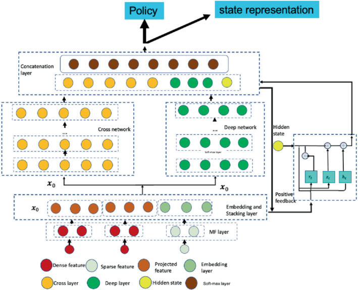
The actor network

2.4.1. Matrix factorization (MF) layer

Due to the heterogeneous data sources, if we model the interactions between cell lines and drugs, we may first project them into the spaces of the same dimension. The easiest way of incorporating drug features is to consider the input as one‐hot encoding. Cell‐line features can be projected into the same dense embedding layer with drug embedding vector for further computation. We have tried initializing the weight matrix for projecting cell line features randomly but noted that it converges slowly. Inspired by Zhang et al ⁵⁵ and Guo et al, ⁵⁶ we decide to use an MF layer for initialization. The input data include dense features such as the cell line gene expression and binary encoding for drugs. The drug response matrix $\mathit{Y}$ can be decomposed into a bias matrix $\mathbf{B}$ and some latent factors for cell lines and drugs:

$$\mathbf{Y}=\mathbf{B}+{\mathbf{UV}}^{\mathrm{T}},\mathbf{U}=\mathit{X}{\mathbf{W}}_{\mathbf{c}},\mathbf{V}=\mathit{D}{\mathbf{W}}_{\mathbf{d}},$$ (13)

where $\mathbf{B}={(b_1,b_2,\dots ,b_M)}^{\top }\in {ℝ}^{N\times M}$, $b_i$ is the bias term for drug $i$; $i=1,\dots ,M$, ${\mathbf{W}}_{\mathbf{c}}\in {ℝ}^{P\times f}$ and ${\mathbf{W}}_{\mathbf{d}}\in {ℝ}^{M\times f}$ are the weight matrices projecting the cell line and drug features into the corresponding latent spaces with dimension $f$ respectively, and are both trainable in a neural network, $\mathit{D}\in {ℝ}^{M\times M}$ which is the identity matrix. Thus $\mathbf{U}={(u_1,u_2,\dots ,u_N)}^{\top }\in {ℝ}^{N\times f}$ denotes the cell lines preference matrix, $\mathbf{V}={(v_1,v_2,\dots ,v_M)}^{\top }\in {ℝ}^{M\times f}$ denotes the drugs' preference matrix. Therefore, the output off the MF layer is the projected dense features $\mathbf{U}$ for each cell line and the embedding matrix $\mathbf{V}$ for the each drug.

2.4.2. Embedding and stacking layer

The input of this layer comes from the output of the MF layer. Then we stack the embedding vectors for each drug along with the dense features of cell lines, together with the cosine similarity score between the cell line's and drugs' latent vectors, into one vector:

$${\mathbf{x}}_0=\left[u^{\top },v_1^{\top },v_2^{\top },\dots ,v_M^{\top },\cos \right],$$ (14)

where $u$ is projected dense features, $v_1,v_2,\dots ,v_M$ is from (13) and cos is the cosine similarity measure between the cell line and the drug. Then we have ${\mathbf{x}}_0={(x_1,x_2,\dots x_d)}^{\top }\in {ℝ}^d$, $d=1+Mf+f+M$, and $x_j$ is the $j$th element of ${\mathbf{x}}_0$. Compared to the Word2Vec ⁵⁷ embedding, we explicitly use the response matrix and the cell line features, which not only generates an embedding for the drug and cell line in the same latent space but also compresses the cell line features.

Importantly, we use the stacking of all the drugs' embedding vector, which is used as the initial state ${\mathbf{s}}_1$. At time step $t$, if drug $j$ is removed from the candidate drugs, we will use a zero vector $(0,0,\dots ,0)\in {ℝ}^f$ to replace $v_j$. It is noted that, although we only use the one‐hot encoding vector for a drug as the sparse vector, sometimes it may not be sufficient, and we can use other side information for drugs. For example, some drug similarity scores from PubChem ⁵⁸ may be used as additional dense features and be projected onto the lower‐dimensional dense layer.

2.4.3. Cross network

For MF‐based ranking methods, it is possible to capture the linear relationship between the latent vectors, but not higher‐order cell line‐drug interactions based on the MF latent factor representation. To capture a higher‐order interactions, we add additional layers in a network to represent interactions as cross‐term features. We denoted the cross term (monomial) as $x_1^{{\alpha }_1}{x}_2^{{\alpha }_2}\dots x_d^{{\alpha }_d}$, with degree $|\mathit{\alpha }|={\sum }_{i=1}^d{\alpha }_i>2$.

To capture higher order interactions, we have the cross network composed of cross layers, where the input is ${\mathbf{x}}_0$ from the stacking and embedding layer in (14), and with each layer having the following formula:

$${\mathbf{x}}_{l+1}={\mathbf{x}}_0{\mathbf{x}}_l^{\top }{\mathbf{w}}_l+{\mathbf{b}}_l+{\mathbf{x}}_l=f\left({\mathbf{x}}_l,{\mathbf{w}}_l,{\mathbf{b}}_l\right)+{\mathbf{x}}_l,$$ (15)

where ${\mathbf{x}}_0$ is the output from (14), ${\mathbf{x}}_l,{\mathbf{x}}_{l+1}$ are the column vectors as the outputs from the $l$th and $(l+1)$th cross layers, respectively; ${\mathbf{w}}_l,{\mathbf{b}}_l$ are the weight and bias parameters in the $l$th layer. By Wang et al, ⁵³ the highest degree of cross terms grows with the layer depth.

It is noted that the cross network is a generalization of MF and so‐called factorization machines ⁵³ by allowing cross terms of any degrees.

In addition, by Wang et al ⁵³ the number of parameters in the cross network is only $d\times L_c\times 2$, where $L_c$ is the number of cross layers. And the output of the cross network is ${\mathbf{x}}_{L_c}$. Accordingly, when we integrate multi‐omic and other high‐dimensional features, the number of parameters in a network model only grows linearly in the number of layers.

2.4.4. Deep network

The deep network is a fully connected feed‐forward neural network, which is good at generalization. Its input is the same as the cross network, which is also ${\mathbf{x}}_0$ from the stacking and embedding layer in (14), and each layer is represented as

$${\mathbf{H}}_{l+1}=f\left(W_l{\mathbf{H}}_l+{\mathbf{b}}_l\right),$$ (16)

where ${\mathbf{H}}_l\in {ℝ}^{n_l}$ and ${\mathbf{H}}_{l+1}\in {ℝ}^{n_{l+1}}$ are the $l$th and $(l+1)$th hidden layers respectively; $W_l\in {ℝ}^{n_{l+1}\times n_l}$ and ${\mathbf{b}}_l\in {ℝ}^{n_{l+1}}$ are the weight matrix and bias vector (as the parameters) for the $l$th layer; and $f(·)$ is the ReLU function. Suppose we have $L_h$ layers for the deep network, then the output is ${\mathbf{H}}_{L_h}$ with the initial input ${\mathbf{x}}_0$. In this fashion, the cross and deep components share the same input, leading to more efficient training, compare. ⁵⁶

2.4.5. GRU layer

In clinical settings, patients' preference or conditions (not captured by given covariates) may change over time, thus we propose using evaluation signals from the ranking process to learn the dynamic hidden preference. The positive drugs represent key information about patients' preferences, that is, which drugs the patients prefer (eg, without minimal side effects). Thus we propose using a GRU layer to memorize the previous evaluation signals, allowing it to remember values over multiple iterations in the sequence. So if the evaluation signal is positive, we can update the GRU layer as the following:

$$\begin{array}{llll}{\mathbf{z}}_t& =\sigma \left(W_z{\mathbf{x}}_t+U_z{\mathbf{H}}_{t-1}+b_z\right),{\mathbf{re}}_t=\sigma \left(W_r{\mathbf{x}}_t+U_r{\mathbf{H}}_{t-1}+b_r\right),& & \\ {\mathbf{H}}_t& =GRU\left({\mathbf{H}}_{t-1},{\mathbf{x}}_t\right)={\mathbf{z}}_t\circ {\mathbf{H}}_{t-1}+\left(1-{\mathbf{z}}_t\right)\circ \tanh \left(W_h{\mathbf{H}}_{t-1}+U_h\left({\mathbf{re}}_t\circ {\mathbf{H}}_{t-1}\right)+b_h\right),& & \end{array}$$

where ${\mathbf{z}}_t$ is the update vector, ${\mathbf{re}}_t$ is the reset gate vector, ${\mathbf{x}}_t$ is the concatenated output from the deep network and cross network at time step t, ${\mathbf{H}}_t$ is the hidden state at time step t, $\circ$ is the Hadamard product and the matrices $W_z,W_h,W_r$, and vectors $b$'s are the unknown weights to be optimized, $\sigma$ is the ReLU activation function. The initial hidden state is set as $\mathbf{\text{0}}$. Then if the current evaluation signal is positive, the output of the hidden state is incorporated into the next combination output layer. We tried to use a pooling layer to represent the dynamic evaluation signal, which gives equal weight to the cell line evaluation signals in the previous time steps; but with the large action space, we noticed that the top 1 drug would dominate the historical evaluation signals, and if the top 1 recommendation was far away from the truth, the actor network would have no chance to adjust the learning process.

2.4.6. Concatenation layer

The concatenation layer concatenates the outputs from the two networks and the GRU layer. We first output the concatenated vector as a state representation to input the critic network, and second apply a standard softmax activation function, yielding the output for policy:

$$\pi \left({\mathbf{a}}_t|{\mathbf{s}}_t\right)=\frac{\exp \left\{{\mathit{\theta }}_{logits}^{\top }{\mathbf{z}}_{m\left(a_t\right)}\right\}}{{\sum }_{a\in A\left(s_t\right)}\exp \left\{{\mathit{\theta }}_{logits}^{\top }{\mathbf{z}}_{m\left(a_t\right)}\right\}},$$ (17)

where ${\mathbf{z}}_{m(a_t)}=\left[{\mathbf{x}}_{L_c}^{\top },{\mathbf{H}}_{L_h}^{\top },{\mathbf{H}}_t\right]$ is the concatenated vector, ${\mathbf{x}}_{L_c}^{\top },{\mathbf{H}}_{L_h}^{\top }$ are the outputs from the cross network and deep network, and ${\mathbf{H}}_t$ is the evaluation signal output from the GRU layer. $m(a(t))$ is the drug index, ${\mathit{\theta }}_{logits}$ is the weight vector for the output layer.

During the training phase of PPORank (as many RL algorithms), the action is often selected according to the current policy estimate; however, to explore (and learn) other potentially more rewarding new actions, it selects an action randomly from the estimated policy distribution. On the other hand, in the testing phase, we just rank the drugs by their predicted scores and select the best one.

2.5. Critic network

The critic network is designed to reduce the variance of the gradients in the policy gradient method, which leverages a deep neural network to approximate the true state value function $V^{{\pi }_{\mathit{\theta }}}({\mathbf{s}}_t)$. The input of the critic network is just the state generated from the actor network in (17), and its output is the state value function $V^{{\pi }_{\mathit{\theta }}}({\mathbf{s}}_t).$ The critic network is jointly learned with the actor network, with the shared state representation as the input from the output of the actor network. We have tried a separate network design, resulting in the divergence of the policy with too many parameters to learn; it is a good way to stabilize training with the shared parameters. The critic is then used to evaluate the policy generated by the actor network and guides the policy gradient. The structure can be found in Figure 2.

FIGURE 2.

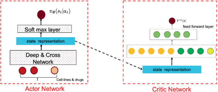
The actor and critic networks

2.6. Learning to rank with Proximal Policy Optimization

The actor‐critic network combines the advantages of value‐based methods and policy gradient to achieve accelerated and stable learning. Yet it is technical and thus is relegated to the Supplementary.

2.7. Top $k$ ranking

In drug recommendation, often only the top one or few matters (as opposed to predicting the exact value of a patient's responses to all drugs). Thus we may be more interested in ranking the top $k$ drugs, instead of ranking all drugs, though the latter may provide more information about the relationships between the drugs and cell lines. The details of our proposed methods are in the Supplementary.

3. EXPERIMENTS

We first conducted our experiments on the cancer screening data sets of GDSC and CCLE. Then we demonstrated the effectiveness of PPORank using simulation data.

3.1. Cancer drug screening data

3.1.1. Datasets

The drug‐screening data for cancer cell lines are obtained from Genomics of Drug Sensitivity in Cancer (GDSC) and Cancer Cell Line Encyclopedia (CCLE). The GDSC database provides a large‐scale drug screening dataset with each $\log ({\text{IC}}_{50})$ value for a drug‐cancer cell line pair. The CCLE database provides genomic, transcriptomic, and epigenomic profiles for more than a thousand cancer cell lines. The GDSC has released a panel of 1001 cancer cell lines (covering 31 cancer types) as well as 265 pharmacological compounds/drugs. ⁴ The cell lines were mostly characterized using gene expression, whole‐exome sequencing, copy number variation, and DNA methylation. As pointed by Coronato et al, ⁶ gene expression data is most informative. Then, we will put more emphasis on our analysis based on gene expression data. To this end, we encode each of the 983 profiled cell lines with the RMA‐normalized (robust multi‐array average) basal expression of 17 737 genes. To extract cell line features from the gene expression profiles, we adopt the method of Reference 13, where we normalize the baseline gene expression values for each gene by computing the fold‐changes compared to the median value across cell lines. According to Reference 12, 1856 essential genes are selected for dimension reduction for each cell line. Then we calculate Pearson's correlation for every pair of cell lines using the expression fold‐changes of these essential genes, among which we select 983 cell line features for the full GDSC dataset.

For the CCLE dataset, 24 drugs and a panel of 1036 human cancer cell lines are available, and we select 491 cancer cell lines for which both drug sensitivity measures and gene expression profile data are available.

Both GDSC and CCLE report drug sensitivity as the logarithm of half maximal inhibitory concentration of a drug on a cell line, $\log ({\text{IC}}_{50})$, which denotes the concentration of the drug/compound required to inhibit the cell growth at 50$\%$; the smaller $\log ({\text{IC}}_{50})$, the more sensitive the cell line to the drug. But the measured $I{C}_{50}$ values are not comparable across different compounds. ⁴ calculated drug‐specific sensitivity (binarization) thresholds for each of the 265 tested drugs. These thresholds were determined using a heuristic outlier detection procedure ⁵⁹ following a previous observation that the majority of cell lines are typically resistant to a given drug. ⁶⁰ Thus, we use these drug‐specific sensitivity thresholds to normalize the data set. Furthermore, as the ranking metric NDCG is only bounded with non‐negative scores, we normalize the sensitivity scores as $-\log ({\text{IC}}_{50}/th{r}_d)+a$, where $th{r}_d$ is the sensitivity threshold of the given drug and $a$ is the maximum normalized $\log (I{C}_{50})$ score across all drugs. After deleting toxic drugs, we have 223 drugs for GDSC and 19 drugs for CCLE.

For drug features, chemical structural information for each drug is available in PubChem. ⁵⁸ We exclude drug samples without PubChem ID in the GDSC database, and we also exclude 15 drugs with the same PubChem IDs, and finally 223 drugs remained. But at the end, for fair comparisons with other baseline methods, drug features are not used.

We employ The Cancer Genome Atlas (TCGA) breast cancer (BRCA) sub‐cohort data to further evaluate whether/how the cell line‐based GDSC results of PPORank generalize to cancer patients. We download the Firehose data run $2016_{-}01_{-}28$ from. ⁶¹ We use the immunohistochemistry annotations to identify HER2 over‐expressed (${\text{HER2}}^{+}$) patients ($n=163$) and triple‐negative breast cancers (TNBCs) patients ($n=116$). Furthermore, we define the BRCA1/2‐mutant (mBRCA) patients as the 37 patients carrying germline loss‐of‐function BRCA1/2 mutations. ⁶² Finally, we use the pipeline proposed by Geeleher et al ⁶³ to harmonize the Level 3 Illumina HiSeq RNA‐seq v2 data (1080 patients) and the GDSC gene expression data.

3.1.2. Baseline methods and evaluations

As described in Section 1, our method (PPORank) is motivated by more efficient healthcare applications: (i) in clinical settings, it is more important to recommend the most sensitive drugs in ranked order, instead of numerically predicting the sensitivity score of a given drug; (ii) a treatment regime is usually characterized after a prolonged and sequential procedure; (iii) currently, many cancer‐related resources covering genotypes, phenotypes, and drug information are available, calling for integrating these multiple data sources for model building; (iv) often only one or few top recommendations are needed (as opposed to all the drugs).

To address the above issues, we will conduct experiments from the following aspects:

• (1)for completeness, we evaluate our method on the full GDSC and CCLE data sets; for a fair comparison, we use the same data sources including only cell line features and drug response matrix and evaluate with NDCG to show long‐term effects, addressing the above issues (i) and (ii);
• (2)to integrate multiple data resources, we also include drug similarity data into the training dataset along with other molecular data: whole‐exome sequencing (WES), copy number variation (CNV), and DNA methylation (MET) data, without any changes to the model structure, addressing issue (iii);
• (3)to address the top $k$ ranking problem of issue (iv), we also evaluate the methods with the $\text{NDCG}@k$ ranking metrics for different values of $k$.

We compare the methods with five‐fold cross‐validation, where each fold of the data is used once for testing while the other four folds are used for training. For each fold, we test completely on unseen cell‐lines. We compare our method, PPORank, against several state‐of‐the‐art and representative ones: a method based on the elastic net regression model ElasticNet (EN), ³ , ⁴ kernel ridge regression (KRR), ⁶⁴ similarity‐regularized matrix factorization (SRMF), ¹² Cancer Drug Response prediction using a Recommender System (CaDRRes), ¹³ and Kernelized Ranking Learning(KRL). ¹⁴ For EN, the model is trained for each drug as described previously ³ , ⁴ using the Elastic Net library in scikit‐learn ($l_1$ ratio =0.5). KRR has been recommended as one of the best‐performing algorithms in a systematic survey ⁷ and was also implemented using the machine learning library‐ scikit‐learn in Python. For SRMF, it goes beyond matrix factorization by also considering drug similarity obtained from chemical structural data and cell line similarity based on their gene expression profiles as regularization terms to avoid over‐fitting; but as described in the article, drug similarity did not improve the prediction performance, so we also ignore drug similarity here. Furthermore, SRMF cannot make predictions on unseen cell lines or patients. For CaDRReS, we set the latent space dimension to be 10. For KRL, we adopt the radial basis function (RBF) kernel, which performs better than the linear kernel, and instead of using cell line similarity features, according to the original paper, we use the RMA‐normalized (robust multi‐array average) basal expression of 17 737 genes as the input cell line features.

3.1.3. Hyper‐parameter tunning

For the baseline methods, the tunning parameters are tuned over grids with five‐fold cross‐validation. For PPORank, we have the following hyper‐parameters, some of which are fixed while others are tuned through the same cross‐validation procedure as for the baseline methods. The cross‐part of the deep‐ and cross network has two cross layers; the deep part of the Deep $\&$ Cross network has three layers with 128, 64, and 32 nodes respectively. For the Deep $\&$ Cross network, we tried some deeper or shallower structures but found that with more layers, the performance did not improve much while a higher dropout rate was needed; to reduce the computational complexity, we ended with the above network structure for our agent policy. For the PPO part, there are two main issues: how many experience episodes ($T$) should the agent gather before updating the policy and how to update an old policy to a new policy. For each trajectory, the cell lines have at most 24 and 265 drugs for the two datasets respectively, so $T$ is set to be 24 for CCLE and 265 for GDSC; for a fair comparison, we do not use the drug fingerprint features here; the numbers of the paralleled actors are 8 for CCLE and 16 for GDSC, mini‐batch size is 16 for both, PPO epoch number $K$ for the surrogate loss (in the Supplementary equation (5)) is 8 for both. For other hyper‐parameters in the clipping loss (in the Supplementary equation (1), which controls the new policy from moving into collapse), the clipping range $ϵ$ is tunned among $\{0.1,0.2,0.3\}$, and the discounting factors $\lambda ,\gamma$ used in the advantage function (in the Supplementary equation (3)) are tuned in grids of $\{0.1,0.2,0.3,\dots ,0.9,0.99\}$, but when evaluated on the whole trajectory's ranking, they are all fixed at the value of 0.95; we only need to tune their values when the evaluation metrics are $\text{NDCG}@k$. The coefficients with the value function and entropy(in the Supplementary equation (5)) are fixed at $c_1=0.5$ and $c_2=0.001$.

3.1.4. Prediction with the full dataset

We use the full GDSC and CCLE data sets with only cell line features to compare the performance of different methods, then we report the average performance based on NDCG through five‐fold cross‐validation. The results are shown in Figure 3. For the CCLE dataset, we can see that our method PPORank performs marginally better than other methods: it gives a mean NDCG of 0.7611, slightly higher than 0.7432 and 0.7468 from linear methods CaDRRes and EN. Note that the total number of the drugs is only 24, so even with unseen cell lines, the candidate drugs have appeared frequently enough in the training set, leading to good performance by both regression methods and static ranking methods. However, for the GDSC dataset, as shown in Figure 3B, the improvement of our PPORank over other methods is much higher. PPORank shows a consistent improvement over all the other methods with the smallest SD (0.003); as a comparison, the second‐best method, CaDRRes, has a much larger SD of 0.011, highlighting the robustness of our proposed method. Note that CaDRRes also uses the NDCG as a loss function, which may explain why it performs second best. To further compare the performance, we will use NDCG$@k$ to show the top $k\ge 1$ selected drugs by each method as to be discussed in Section 3.3 (where it is shown that PPORank demonstrates larger performance gains over CaDRRes and other methods).

FIGURE 3.

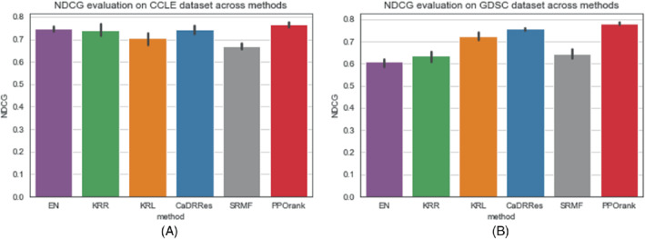
Mean NDCG values by five‐fold cross‐validation (with 1 SD as error bars). (A) NDCG values using full CCLE data set; (B) NDCG values using full GDSC data set

To compare the performance between our proposed RL and DNN‐based supervised learning, we also developed and trained a DNN using an approximate NDCG as the loss function ⁶⁵ based on the GDSC data. Figure 4 shows that after 600 epochs, PPORank approaches the performance of the DNN. It suggests that the improvement of PPORank over other methods perhaps mainly comes from two sources: its highly non‐linear model and its direct use of NDCG as its target loss function.

FIGURE 4.

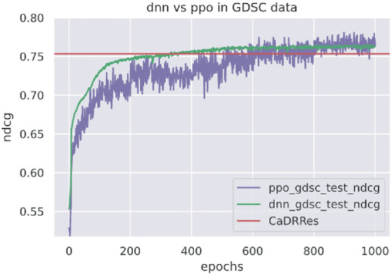
DNN and PPORank's performance using $NDCG$ on the GDSC data

3.1.5. Prediction with other types of cell line features

We use the Gaussian kernel ⁶⁶ to summarize side information from other omic data sources: for each cell line $c$, $\mathbf{K}\left({\mathbf{x}}_{\mathbf{c}},{\mathbf{x}}_{{\mathbf{c}}^{\prime }}\right)=\exp \left(-{‖{\mathbf{x}}_{\mathbf{c}}-{\mathbf{x}}_{{\mathbf{c}}^{\prime }}‖}^2/2{\sigma }^2\right)$, where ${\mathbf{x}}_{\mathbf{c}}$ and ${\mathbf{x}}_{{\mathbf{c}}^{\prime }}$ denote the feature vectors of two cell lines in the form of (i) whole‐exome sequencing (WES), (ii) copy number variation (CNV), or (iii) DNA methylation (MET) data, and $\sigma$ is the kernel width of the Gaussian kernel. For simplicity, we heuristically determine the kernel width using the “median trick,” setting the width as the reciprocal of the median squared Euclidean distance among all training sample pairs. In this fashion, we generate an $N\times N$ kernel matrix $\mathbf{K}$ for each additional data type, where $N$ is the number of cell lines. We treat each row of $\mathbf{K}$ as a feature vector of length $N$ for the corresponding omic data and cell‐line, which can be combined with the original cell‐line features to incorporate the use of other omic data.

Since our method is based on DNNs, it is quite flexible to accommodate other data sources: we add an (MLP) subnetwork to project other high‐dimensional features to a low‐dimension space before feeding its output to the stacking layer. As gene expression (GEX) data is known to be informative, we use the following cell line features (1) GEX+WES, (2) GEX+CNV, (3) GEX+MET respectively to show how performance may change; more details about these features can be found in Appendix Table A1. Figure 5 compares the performance in NDCG across using these three additional types of features. In agreement with the findings from a drug sensitivity collaborative competition, ⁶ gene expression is confirmed to be the most predictive data type regardless of the method being employed, since it shows almost no improvement with the additional CNV or WES data and only slight improvement with the MET data; these results are also consistent with some previous studies supporting that MET data are informative to cancer. ⁶⁷

FIGURE 5.

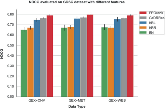
Mean NDCG values by five‐fold cross‐validation on the GDSC data with different types of omic data features

3.2. Sequential learning and prediction

One distinct feature of RL is its sequential learning. Although all the data from GDSC are available at the time of training, we mimic a realistic situation by starting RL with a subset of the available data. We begin with 50$\%$ of all the cell lines in the GDSC data at start time $t_0$. As the model uses all the drugs for embedding learning in our deep $\&$ cross net, we consider all the drugs at time $t_0$; we evaluate the method at each following time point using the independent test data. Specifically, at time point $t_0+1$, we add 20 cell lines as new data and run the RL algorithm based on the feedback of the newly added data; after the convergence, we evaluate its performance based on the (unseen) test data. Then we add another 20 cell lines as new data, and repeat the process. To save time, at each time point we start RL with the estimated model (ie, its estimated parameters) obtained from the previous run (or time point), then update the model with the new incoming cell lines. Figure 6 displays the results of applying RL on the GDSC test data, starting at $t_0$ with only 50% of the whole training data and subsequently adding 20 more cell lines at each time point until we use up all the GDSC training data. As expected, as more data are added, overall the performance of RL improves. It is confirmed that RL performs well in the realistic set‐up for sequential learning.

FIGURE 6.

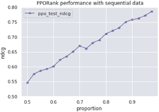
PPORank performance on GDSC with sequential data

3.3. Prediction with top $k$ ranking

To show the ability of the PPORank model for ranking the top $k$ most sensitive drugs across cell lines, we use the full CCLE and GDSC data sets respectively to compared the methods in terms of $\text{NDCG}@k$ with $k\in \{1,5,10\}$; with $k=1$, one is to select the most sensitive drug. As shown in Figure 7, PPORank performs best consistently; its improvements over other methods are more obvious for the GDSC data. From Section 2.1,

$$\text{NDCG}@\{k+1\}-\text{NDCG}@k=\frac{\left[\frac{2^{f_{{\mathit{\pi }}^{-1}(k+1)}}-1}{{\log }_2(k+2)}\times Z_k-DCG@k\times \frac{2^{y_{k+1}}-1}{{\log }_{k+2}}\right]}{Z_k{Z}_{k+1}},$$

where $Z_k$ is a normalized factor that $Z_k\ge \text{DCG}@k$. So, when $\frac{2^{f_{{\mathit{\pi }}^{-1}(k+1)}}-1}{{\log }_2(k+2)}\times Z_k$ is larger than $\text{DCG}@k\times \frac{2^{y_{k+1}}-1}{{\log }_{k+2}}$, $\text{NDCG}@k$ increases in $k$. In practice, depending on data, an increasing trend may not be seen in all circumstances for a top $k$ ranking problem.

FIGURE 7.

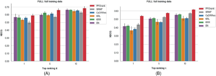
$\text{NDCG}@k$ values with the full CCLE or GDSC data for different $k$; the error bars show one SD based on three‐fold cross‐validation. (A) $\text{NDCG}@k$ with the CCLE data; (B) $\text{NDCG}@k$ with the GDSC data

3.4. External validation with TCGA breast cancer cohort

To show the generalization ability of PPORank, we show that drug ranks predicted with PPORank trained on cell lines from GDSC are correlate with patient response to treatment in a TCGA breast cancer cohort. ⁶⁸ We follow the data preprocessing of Reference 63 to harmonize the gene expression profiles measured by RNA‐seq in TCGA and by micro‐arrays in GDSC. In this way, they were able to train ridge regression models on the GDSC cell lines and use these models to “impute” drug response for the TCGA patients. They also showed that ${\text{HER2}}^{+}$ TCGA‐BRCA patients were predicted to be more sensitive to lapatinib, a first‐line therapy for ${\text{HER2}}^{+}$ patients, ⁶⁹ than other patients. Here we follow the idea of using molecular subtypes to evaluate PPORank's recommendations.

We compare lapatinib and four PARP 1/2 inhibitors (PARPi), veliparib, olaparib, talazoparib, and rucaparib, some of which have shown promising therapeutic response in BRCA1/2‐mutant (mBRCA) tumors. ⁷⁰ In our experiments, lapatinib is ranked higher than all four PARPi for 150 (92%) of the 163 ${\text{HER2}}^{+}$ patients; in contrast, for mBRCA TNBC , lapatinib is ranked higher than PARPi only 22$\%$. Table 1 shows how lapatinib is recommended as compared to the overall and individual PARPi treatments. To show the robustness of our proposed method, we retrain the model 10 times with a subset of 100 drugs (but with lapatinib and PARPi always included) randomly selected from the 200+ available drugs in the GDSC data. It is confirmed that PPORank's recommendations are indeed statistically different from that of a random recommendation (the unpaired $t$‐test with $\text{mean P‐value}=10^{-11}$ for ${\text{HER2}}^{+}$ and $\text{P‐value}=10^{-27}$ for mBRCA TNBC patients). Furthermore, when we apply the unpaired $t$‐test to compare random recommendations with each of the four individual PARPi treatments, the results were statistically significant ($\text{P‐value}\le .005$) except for rucaparib ($\text{P‐value}=.13$). This suggests no recommendation of rucaparib to mBRCA TNBC patients, which is in agreement with a recent clinical trial's ⁷¹ conclusion that the efficacy of rucaparib was not established and it required further investigation.

TABLE 1.

PPORank's recommendation rates of lapatinib for the TCGA patients with two different breast cancer subtypes

Recommendation	${\text{HER2}}^{+}$ ($n=163$)	mBRCA ($n=9$)
lapatinib $>$ PARPi	0.92	0.22
lapatinib $>$ veliparib	0.95	0.22
lapatinib $>$ olaparib	0.94	0.44
lapatinib $>$ talazoparib	0.92	0.22
lapatinib $>$ rucaparib	0.95	0.44

3.5. Simulations

3.5.1. Primary simulations

To compare our method with other baseline methods, we first construct the response matrix with information from the cell lines. Now consider 100 drugs and 1000 cell lines with 2000 features for cell lines thus $\mathit{X}\in {ℝ}^{1000\times 2000}$. As pointed out by Cortes‐Ciriano et al ¹² and Seashore‐Ludlow et al ⁷² drug pairs within the same cluster of chemical fingerprints can show similar inhibitory effects on the same cell line. So we generate $\mathit{X}$ with 2000 features from 10 clusters with a cluster size of $\{480,380,300,240,190,150,120,90,40,10\}$; the features belong to the same cluster are correlated. Each feature is generated from a uniform distribution. The correlation matrix of $\mathit{X}$ can be seen from Figure 8A. We design a weight matrix $\mathit{W}\in {ℝ}^{2000\times 100}$ with 10 clusters each with an equal size of 10; for each cluster, the weight is generated from a standard normal distribution as shown in Figure 8B. For each simulated cell line, a maximum number of 100 drugs need to be ranked.

FIGURE 8.

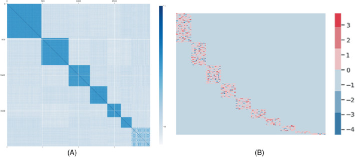
Simulation setups: (A) The correlation matrix of the simulated cell lines features with 10 clusters; (B) the weight matrix $\mathit{W}$ with 10 clusters

We generate the response matrix $\mathit{Y}\in {ℝ}^{1000\times 100}$ from one of the three models:

1. $\mathit{Y}=\mathit{\mu }+\mathit{ϵ}=0.2\times \mathit{X}\mathit{W}+\mathit{ϵ},$
2. $\mathit{Y}=\mathit{\mu }+\mathit{ϵ}=0.15\times {\mathit{X}}^3\mathit{W}+0.15\times \mathit{X}\mathit{W}+\mathit{ϵ},$
3. $\mathit{Y}=\mathit{\mu }+\mathit{ϵ}=0.1\times \exp (\mathit{X})\mathit{W}+0.1\times {\mathit{X}}^3\mathit{W}+\mathit{ϵ},$

representing linear, non‐linear (cubic) and highly non‐linear (exponential) scenarios, and $\mathit{ϵ}$ is a Gaussian noise. Here, instead of using the original Pearson correlation matrix as in the CaDRRes paper, ¹³ we use the original cell line features from $\mathit{X}$. We define the $(i,j)$th element of ${\mathit{Y}}_{true}$ as the true mean response for the $i$th cell line given the $j$th drug. As NDCG is commutable only when the relevance label is non‐negative, we set a response value $\mathit{Y}$ as missing if it is negative. We also set 50$\%$ of the remaining response values as missing. To distinguish between sensitive and nonsensitive drugs, we use the median response of all the cell lines to a specific drug as the threshold. If a response value is larger than the threshold, we take it as sensitive/positive; otherwise, it is nonsensitive/negative. During training, if we have a nonsensitive drug in a ranking position while there are other sensitive candidate drugs to be selected, we take it as a negative evaluation signal and otherwise as a positive evaluation signal.

We also compare DNN with PPORank in the linear and exponential scenarios with a sample size of 1000. From Figure 9a, we can see that in the linear scenario, DNN reaches the stable and perhaps optimal performance sooner, while PPORank fluctuates but reaches a relatively stable plateau after 1000 epochs. As our sample size is only 1000, while the number of the parameters in PRORank is almost 10 times the sample size, it needs to sample more trajectories in a long run to reach and even slightly exceeds the DNN's performance. As expected, both DNN and PPORank perform worse than the linear method of “CaDDRes.” On the other hand, for the exponential scenario, Figure 9B shows faster convergence by both DNN and PPORank than that in the linear scenario, presumably because we are using nonlinear networks to describe the true nonlinear relationship.

FIGURE 9.

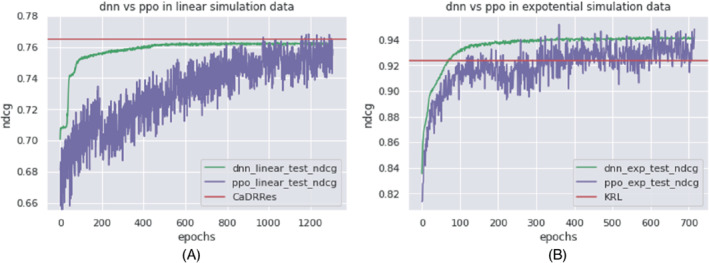
Performance of DNN and PPORank in terms of $NDCG$ in two simulation scenarios. (A) Simulation scenario (1); (B) simulation scenario (3)

Then we compare our PPORank with and without positive evaluation signals (PPO vs PPO‐w/o), respectively, and other baseline methods, using simulated data as shown in Table 2. The sample size for each scenario is 1000 or 10 000. We do not include SRMF as it requires drug similarity, though the GDSC data application shows that drug similarity does not improve performance much. From the NDCG values in scenario (1), where the cell lines' features have a linear effect on drug response, MF‐based methods can capture the linear relationship and perform well. After increasing the sample size to 10 000, PPORank performs best, presumably because it is the only one targeting NDCG, the evaluation criterion being used, as its loss function. For scenario (2), we reach the same conclusion as for scenario (1). In contrast, for scenario (3) with a highly non‐linear true model, PPORank performs best with either sample size (Table 2).

TABLE 2.

Mean NDCG (SD) in the primary simulations

	Scenario 1		Scenario 2		Scenario 3
	n=1000	n=10 000	n=1000	n=10 000	n=1000	n=10 000
EN	0.793 (0.03)	0.801 (0.02)	0.593 (0.05)	0.621 (0.04)	0.890 (0.04)	0.905 (0.03)
KRR	0.774 (0.04)	0.769 (0.07)	0.532 (0.05)	0.582 (0.05)	0.882 (0.06)	0.901 (0.04)
KRL	0.783 (0.02)	0.793 (0.01)	0.625 (0.02)	0.647 (0.03)	0.920 (0.03)	0.927 (0.02)
CaDRRes	0.809 (0.02)	0.824 (0.02)	0.632 (0.03)	0.682 (0.02)	0.922 (0.02)	0.931 (0.02)
ppo‐w/o	0.798 (0.07)	0.811 (0.10)	0.670 (0.04)	0.693 (0.01)	0.940 (0.03)	0.948 (0.04)
PPORank	0.790 (0.06)	0.832 (0.04)	0.651 (0.02)	0.705 (0.05)	0.941 (0.05)	0.959 (0.03)

Note: The boldfaced values show the best performances.

3.5.2. Secondary simulations

To consider more complex relationships between cell lines and drugs, we design the following simulation setup. Suppose we have 40 drugs and 1000 cell lines, the cell line feature matrix $\mathit{X}\in {ℝ}^{1000\times 2000}$ is the same as in the previous static simulation setup. The weight matrix $\mathit{W}\in {ℝ}^{2000\times 100}$ is also the same as before. However, the drug response varies with the drug. For the first 20, next 10, and final 10 drugs, we have $\mathit{Y}=0.2\times \mathit{X}\mathit{W}+\mathit{ϵ}$, $\mathit{Y}=0.15\times {\mathit{X}}^3\mathit{W}+0.15\times \mathit{X}\mathit{W}+\mathit{ϵ}$, and $\mathit{Y}=0.2\times \exp (\mathit{X})\mathit{W}-0.1\times {\mathit{X}}^3\mathit{W}+\mathit{ϵ}$, respectively.

We evaluate the performances with the sample size $n=1000$ and $n=10000$. From Table 3 we can see that PPORank performs best.

TABLE 3.

Mean NDCG (SD) for the secondary simulations

	$n=1000$		$n=10000$
EN	0.645 (0.08)		0.679 (0.07)
KRR	0.641 (0.11)		0.650 (0.10)
KRL	0.689 (0.09)		0.707 (0.08)
CaDRRes	0.647 (0.11)		0.689 (0.09)
ppo‐w/o	0.701 (0.11)		0.713 (0.12)
PPORank	0.721 (0.11)		0.732 (0.09)

Note: The boldfaced values show the best performances.

4. CONCLUSIONS AND DISCUSSION

In this article, we have proposed a novel personalized ranking system called Proximal Policy Optimization Ranking (PPORank), which ranks drugs/treatments based on their predicted effects per cell line (or patient). It makes recommendations directly based on the ranking of the drugs, instead of on predicting some drug‐specific responses per se, for example, their $\log ({\text{IC}}_{50})$) values, as adopted by other existing methods. Hence this policy‐based learning framework directly optimizes the target evaluation metric using the policy gradient algorithm. Furthermore, the evaluation metric NDCG is optimized by leveraging information from all the ranks. In the implementation, we have adopted some state‐of‐the‐art techniques in DRL as briefly discussed below. By using a Deep$\&$Cross network to parametrize the policy, we can learn the interactions between cell lines and drugs efficiently, and it can be extended to integrate other data sources. In particular, we use a GRU layer to incorporate the dynamic evaluation signal from cell lines and reinforce the policy with evaluation signals. Variance reduction is realized by using the actor‐critic framework, where the actor network learns the states from the input and feeds it to the critic network to evaluate the current policy. To handle the sample inefficiency problem of policy gradient methods, we use the PPO algorithm with multiple epochs of stochastic gradient ascent to update the policy. As proofs‐of‐concept, we have applied our method to two large‐scale cancer drug screening datasets for personalized drug discovery. With the limited data and high dimensions of the states and actions, our method has shown superior performance over other methods. In particular, our method demonstrates its promising and clinically meaningful performance when the learning algorithm trained on the cell line drug screening data is applied to a TCGA breast cancer cohort. Most importantly, our method, as any RL method, can be more efficiently applied in practice: it learns sequentially and continuously as the data accrue; in contrast, existing supervised learning and many DTR methods would require finishing collecting data (from either a randomized experiment or an observational study) first before learning personalized drug ranking, which would be more resource‐ and time‐consuming. This feature of our method would be most useful for more efficient drug discovery as for our real data applications, and possibly for behavioral interventions in mHealth or selecting experimental drugs for patients with incurable or terminal diseases. In addition, through transfer learning, our proposed RL method can take advantage of existing data and be trained a priori before being applied to and fine‐tuned by future clinical data. Finally, an important aspect of our proposed RL method is its active learning and dynamic interaction with individuals: the learning algorithm would suggest the best treatment/intervention based on its current ranking to an individual, then learn from the outcome, for example, in mHealth applications. Due to lack of data, we have not explored this aspect. This is a distinct and attractive feature unique to RL, but not to supervised learning.

On the other hand, there are some challenges remaining before DRL being applied more generally for health care in practice. First, due to the “data‐hungry” nature of both DL and RL (and thus DRL), more data efficient algorithms are urgently needed. Transfer learning mentioned earlier can also help. Second, the interpretability of a DL model as a black‐box needs to be improved. Both topics have generated extensive interests and intensive research in the DL community, which will hopefully lead to some breakthroughs in a near future. In summary, our proposed and possibly other DRL‐based methods are promising for precision medicine, and worth further investigation.

Supporting information

Data S1: Supplementary material

1.

Table A1 lists main mathematical notations used throughout this article. The main PPORank algorithm and its episode‐sampling component are also described as two algorithms (Algorithms 1 and 2).

Algorithm 1. Sample an episode.

1.

Algorithm 2. PPORank.

1.

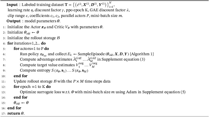
TABLE A1.

Mathematical notations

Meaning	Notation
Cell‐line	$c,$ or $c^{(i)}$ a
Number of training cell lines	$N$
Maximum number of drugs for each cell line	M
Feature vector of cell line $c^{(i)}$	$X^{(i)}$ or $X$
Drug $u$ is more sensitive than drug $v$	$d_u\succ d_v$
Number of drugs associated with cell line $c^{(i)}$	$M_i$
Feature vector or binary features of a drug $j$ associated with cell line $c^{(i)}$	${\mathbf{d}}_j^{(i)}$ or ${\mathbf{d}}_j$
Embedding vector of a drug $j$ associated with cell line $c^{(i)}$	${\mathbf{d}}_{embed,j}^{(i)}$ or ${\mathbf{d}}_{embed,j}$
Feature vectors or binary indexes of drugs associated with cell line $c^{(i)}$	$D^{(i)}={\{{\mathbf{d}}_j^{(i)}\}}_{j=1}^{M_i}$ or $D$
Remaining drugs associated with cell line $c^{(i)}$ at time step t	$D_t^{(i)}$ or $D_t$
Ground truth response score of a drug $j$ associated with cell line $c^{(i)}$	$y_j^{(i)}$ or $y_j$
Ground truth permutation (ranking list) for drugs associate with cell line $c$	${\mathit{\pi }}^{\ast }$
Original drug index of the $j$th element in permutation $\mathit{\pi }$	${\mathit{\pi }}^{-1}(j)$
Ranking position of drug $j$ in permutation $\mathit{\pi }$	$\mathit{\pi }(j)$

^aThe superscript $\{i\}$ indicates the associate cell line $c^{(i)}$, if it is missing, it can be applied to general case that is associated with cell line $c$.

Liu M, Shen X, Pan W. Deep reinforcement learning for personalized treatment recommendation. Statistics in Medicine. 2022;41(20):4034–4056. doi: 10.1002/sim.9491

DATA AVAILABILITY STATEMENT

The code and the real data being used are available on GitHub at https://github.com/mylzwq/PPORank.

REFERENCES

- 1. Kosorok MR, Laber EB. Precision medicine. Annu Rev Stat Appl. 2019;6:263‐286. [DOI] [PMC free article] [PubMed] [Google Scholar]
- 2. Menden MP, Iorio F, Garnett M, et al. Machine learning prediction of cancer cell sensitivity to drugs based on genomic and chemical properties. PLoS One. 2013;8(4):e61318. [DOI] [PMC free article] [PubMed] [Google Scholar]
- 3. Barretina J, Caponigro G, Stransky N, et al. The cancer cell line encyclopedia enables predictive modelling of anticancer drug sensitivity. Nature. 2012;483(7391):603‐607. [DOI] [PMC free article] [PubMed] [Google Scholar]
- 4. Iorio F, Knijnenburg TA, Vis DJ, et al. A landscape of pharmacogenomic interactions in cancer. Cell. 2016;166(3):740‐754. [DOI] [PMC free article] [PubMed] [Google Scholar]
- 5. Weinstein JN, Collisson EA, Mills GB, et al. The cancer genome atlas pan‐cancer analysis project. Nat Genet. 2013;45(10):1113‐1120. [DOI] [PMC free article] [PubMed] [Google Scholar]
- 6. Costello JC, Heiser LM, Georgii E, et al. A community effort to assess and improve drug sensitivity prediction algorithms. Nat Biotechnol. 2014;32(12):1202‐1212. [DOI] [PMC free article] [PubMed] [Google Scholar]
- 7. Jang IS, Neto EC, Guinney J, Friend SH, Margolin AA. Systematic Assessment of Analytical Methods for Drug Sensitivity Prediction from Cancer Cell Line Data. Pac Symp Biocomput. 2014:63‐74. [PMC free article] [PubMed] [Google Scholar]
- 8. Azuaje F. Computational models for predicting drug responses in cancer research. Brief Bioinform. 2017;18(5):820‐829. [DOI] [PMC free article] [PubMed] [Google Scholar]
- 9. Aben N, Vis DJ, Michaut M, Wessels LF. TANDEM: a two‐stage approach to maximize interpretability of drug response models based on multiple molecular data types. Bioinformatics. 2016;32(17):i413‐i420. [DOI] [PubMed] [Google Scholar]
- 10. Gupta S, Chaudhary K, Kumar R, et al. Prioritization of anticancer drugs against a cancer using genomic features of cancer cells: A step towards personalized medicine. Sci Rep. 2016;6:23857. [DOI] [PMC free article] [PubMed] [Google Scholar]
- 11. Cortés‐Ciriano I, van Westen GJ, Bouvier G, et al. Improved large‐scale prediction of growth inhibition patterns using the NCI60 cancer cell line panel. Bioinformatics. 2016;32(1):85‐95. [DOI] [PMC free article] [PubMed] [Google Scholar]
- 12. Wang L, Li X, Zhang L, Gao Q. Improved anticancer drug response prediction in cell lines using matrix factorization with similarity regularization. BMC Cancer. 2017;17(1):513. [DOI] [PMC free article] [PubMed] [Google Scholar]
- 13. Suphavilai C, Bertrand D, Nagarajan N. Predicting cancer drug response using a recommender system. Bioinformatics. 2018;34(22):3907‐3914. [DOI] [PubMed] [Google Scholar]
- 14. He X, Folkman L, Borgwardt K. Kernelized rank learning for personalized drug recommendation. Bioinformatics. 2018;34(16):2808‐2816. [DOI] [PMC free article] [PubMed] [Google Scholar]
- 15. Ding MQ, Chen L, Cooper GF, Young JD, Lu X. Precision oncology beyond targeted therapy: combining omics data with machine learning matches the majority of cancer cells to effective therapeutics. Mol Cancer Res. 2018;16(2):269‐278. doi: 10.1158/1541-7786.MCR-17-0378 [DOI] [PMC free article] [PubMed] [Google Scholar]
- 16. Yuan H, Paskov I, Paskov H, González AJ, Leslie CS. Multitask learning improves prediction of cancer drug sensitivity. Sci Rep. 2016;6(1):1‐11. [DOI] [PMC free article] [PubMed] [Google Scholar]
- 17. Chang Y, Park H, Yang HJ, et al. Cancer drug response profile scan (CDRscan): a deep learning model that predicts drug effectiveness from cancer genomic signature. Sci Rep. 2018;8(1):8857. doi: 10.1038/s41598-018-27214-6 [DOI] [PMC free article] [PubMed] [Google Scholar]
- 18. Robins JM. Correcting for non‐compliance in randomized trials using structural nested mean models. Commun Stat Theory Methods. 1994;23(8):2379‐2412. [Google Scholar]
- 19. Robins JM. Causal inference from complex longitudinal data; 1997:69‐117; Springer.
- 20. Murphy SA. Optimal dynamic treatment regimes. J Royal Stat Soc Ser B (Stat Methodol). 2003;65(2):331‐355. [Google Scholar]
- 21. Zhao Y, Kosorok MR, Zeng D. Reinforcement learning design for cancer clinical trials. Stat Med. 2009;28(26):3294‐3315. [DOI] [PMC free article] [PubMed] [Google Scholar]
- 22. Zhao Y, Zeng D, Socinski MA, Kosorok MR. Reinforcement learning strategies for clinical trials in nonsmall cell lung cancer. Biometrics. 2011;67(4):1422‐1433. [DOI] [PMC free article] [PubMed] [Google Scholar]
- 23. Zhao YQ, Zeng D, Laber EB, Kosorok MR. New statistical learning methods for estimating optimal dynamic treatment regimes. J Am Stat Assoc. 2015;110(510):583‐598. [DOI] [PMC free article] [PubMed] [Google Scholar]
- 24. Lei H, Nahum‐Shani I, Lynch K, Oslin D, Murphy SA. A "SMART" design for building individualized treatment sequences. Annu Rev Clin Psychol. 2012;8:21‐48. [DOI] [PMC free article] [PubMed] [Google Scholar]
- 25. Moodie EE, Chakraborty B, Kramer MS. Q‐learning for estimating optimal dynamic treatment rules from observational data. Can J Stat. 2012;40(4):629‐645. [DOI] [PMC free article] [PubMed] [Google Scholar]
- 26. Zhang B, Tsiatis AA, Laber EB, Davidian M. Robust estimation of optimal dynamic treatment regimes for sequential treatment decisions. Biometrika. 2013;100(3):681‐694. [DOI] [PMC free article] [PubMed] [Google Scholar]
- 27. Zhang Y, Laber EB, Davidian M, Tsiatis AA. Interpretable dynamic treatment regimes. J Am Stat Assoc. 2018;113(524):1541‐1549. [DOI] [PMC free article] [PubMed] [Google Scholar]
- 28. Schulte PJ, Tsiatis AA, Laber EB, Davidian M. Q‐and A‐learning methods for estimating optimal dynamic treatment regimes. Stat Sci Rev J Inst Math Stat. 2014;29(4):640. [DOI] [PMC free article] [PubMed] [Google Scholar]
- 29. Zhao Y, Zeng D, Rush AJ, Kosorok MR. Estimating individualized treatment rules using outcome weighted learning. J Am Stat Assoc. 2012;107(499):1106‐1118. [DOI] [PMC free article] [PubMed] [Google Scholar]
- 30. Liu M, Shen X, Pan W. Outcome weighted ‐learning for individualized treatment rules. Stat. 2021;10(1):e343. [DOI] [PMC free article] [PubMed] [Google Scholar]
- 31. Zhou X, Mayer‐Hamblett N, Khan U, Kosorok MR. Residual weighted learning for estimating individualized treatment rules. J Am Stat Assoc. 2017;112(517):169‐187. [DOI] [PMC free article] [PubMed] [Google Scholar]
- 32. Ertefaie A, Strawderman RL. Constructing dynamic treatment regimes over indefinite time horizons. Biometrika. 2018;105(4):963‐977. [Google Scholar]
- 33. Luckett DJ, Laber EB, Kahkoska AR, Maahs DM, Mayer‐Davis E, Kosorok MR. Estimating dynamic treatment regimes in mobile health using V‐learning. J Am Stat Assoc. 2020;115(530):692‐706. [DOI] [PMC free article] [PubMed] [Google Scholar]
- 34. Coronato A, Naeem M, De Pietro G, Paragliola G. Reinforcement learning for intelligent healthcare applications: a survey. Artif Intell Med. 2020;109:101964. [DOI] [PubMed] [Google Scholar]
- 35. Yu C, Liu J, Nemati S, Yin G. Reinforcement learning in healthcare: A survey. ACM Comput Surv (CSUR). 2021;55(1):1‐36. [Google Scholar]
- 36. Zhou SK, Le HN, Luu K, Nguyen HV, Ayache N. Deep reinforcement learning in medical imaging: A literature review. Med Image Anal. 2021;73:102193. [DOI] [PubMed] [Google Scholar]
- 37. Schulman J, Wolski F, Dhariwal P, Radford A, Klimov O. Proximal policy optimization algorithms. arXiv preprint arXiv:1707.06347, 2017.
- 38. Figueiredo Prudencio R, Maximo MR, Luna CE. A survey on offline reinforcement learning: taxonomy, review, and open problems. arXiv e‐prints 2022: arXiv–2203. [DOI] [PubMed]
- 39. Liu S, See KC, Ngiam KY, et al. Reinforcement learning for clinical decision support in critical care: comprehensive review. J Med Internet Res. 2020;22(7):e18477. [DOI] [PMC free article] [PubMed] [Google Scholar]
- 40. Murphy SA. An experimental design for the development of adaptive treatment strategies. Stat Med. 2005;24(10):1455‐1481. [DOI] [PubMed] [Google Scholar]
- 41. Humphrey K. Using Reinforcement Learning to Personalize Dosing Strategies in a Simulated Cancer Trial with High Dimensional Data [Master's Theses]. The University of Arizona; 2017.
- 42. Yauney G, Shah P. Reinforcement learning with action‐derived rewards for chemotherapy and clinical trial dosing regimen selection; 2018:161‐226; PMLR.
- 43. Tseng HH, Luo Y, Cui S, Chien JT, Ten Haken RK, Naqa IE. Deep reinforcement learning for automated radiation adaptation in lung cancer. Med Phys. 2017;44(12):6690‐6705. [DOI] [PMC free article] [PubMed] [Google Scholar]
- 44. Peng X, Ding Y, Wihl D, et al. Improving Sepsis Treatment Strategies by Combining Deep and Kernel‐Based Reinforcement Learning. American Medical Informatics Association (AMIA) 2018 Annual Symposium; 2018;887‐896. [PMC free article] [PubMed] [Google Scholar]
- 45. Weng WH, Gao M, He Z, Yan S, Szolovits P. Representation and reinforcement learning for personalized glycemic control in septic patients. arXiv preprint arXiv:1712.00654; 2017.
- 46. Wang L, Zhang W, He X, Zha H. Supervised reinforcement learning with recurrent neural network for dynamic treatment recommendation. Proceedings of the 24th ACM SIGKDD International Conference on Knowledge Discovery & Data Mining; 2018:2447‐2456; ACM, New York.
- 47. Prasad N, Cheng LF, Chivers C, Draugelis M, Engelhardt BE. A reinforcement learning approach to weaning of mechanical ventilation in intensive care units. arXiv preprint arXiv:1704.06300, 2017.
- 48. Sutton RS, Barto AG. Reinforcement Learning: An Introduction. Cambridge, MA: MIT Press; 2018. [Google Scholar]
- 49. Järvelin K, Kekäläinen J. Cumulated gain‐based evaluation of IR techniques. ACM Trans Inf Syst (TOIS). 2002;20(4):422‐446. [Google Scholar]
- 50. Wei Z, Xu J, Lan Y, Guo J, Cheng X. Reinforcement learning to rank with Markov decision process. Proceedings of the 40th International ACM SIGIR Conference on Research and Development in Information Retrieval; 2017:945‐948; ACM, New York.
- 51. Clarke CL, Kolla M, Cormack GV, et al. Novelty and diversity in information retrieval evaluation. Proceedings of the 31st Annual International ACM SIGIR Conference on Research and Development in Information Retrieval; 2008:659‐666; ACM, New York.
- 52. Sutton RS, McAllester DA, Singh SP, Mansour Y. Policy gradient methods for reinforcement learning with function approximation. Advances in Neural Information Processing Systems. 2000:1057‐1063. [Google Scholar]
- 53. Wang R, Fu B, Fu G, Wang M. Deep & cross network for ad click predictions. Proceedings of the ADKDD'17. New York: ACM; 2017:1‐7. [Google Scholar]
- 54. Cho K, Van Merriënboer B, Gulcehre C, et al. Learning phrase representations using RNN encoder‐decoder for statistical machine translation. arXiv preprint arXiv:1406.1078, 2014.
- 55. Zhang W, Du T, Wang J. Deep learning over multi‐field categorical data. Proceedings of the European Conference on Information Retrieval; 2016:45‐57; Springer, New York.
- 56. Guo H, Tang R, Ye Y, Li Z, He X. DeepFM: a factorization‐machine based neural network for CTR prediction. arXiv preprint arXiv:1703.04247, 2017.
- 57. Mikolov T, Chen K, Corrado G, Dean J. Efficient estimation of word representations in vector space. arXiv preprint arXiv:1301.3781, 2013.
- 58. Kim S, Thiessen PA, Bolton EE, et al. PubChem substance and compound databases. Nucl Acids Res. 2016;44(D1):D1202‐D1213. [DOI] [PMC free article] [PubMed] [Google Scholar]
- 59. Knijnenburg TA, Klau GW, Iorio F, et al. Logic models to predict continuous outputs based on binary inputs with an application to personalized cancer therapy. Sci Rep. 2016;6(1):1‐14. [DOI] [PMC free article] [PubMed] [Google Scholar]
- 60. Garnett MJ, Edelman EJ, Heidorn SJ, et al. Systematic identification of genomic markers of drug sensitivity in cancer cells. Nature. 2012;483(7391):570‐575. [DOI] [PMC free article] [PubMed] [Google Scholar]
- 61. Head T, Carcinoma NSC. Broad institute TCGA genome data analysis center. Firehose Stddata__2016_01_28 run 2016.
- 62. Maxwell KN, Wubbenhorst B, Wenz BM, et al. BRCA locus‐specific loss of heterozygosity in germline BRCA1 and BRCA2 carriers. Nat Commun. 2017;8(1):1‐11. [DOI] [PMC free article] [PubMed] [Google Scholar]
- 63. Geeleher P, Zhang Z, Wang F, et al. Discovering novel pharmacogenomic biomarkers by imputing drug response in cancer patients from large genomics studies. Genome Res. 2017;27(10):1743‐1751. [DOI] [PMC free article] [PubMed] [Google Scholar]
- 64. Murphy KP. Machine Learning: A Probabilistic Perspective. Cambridge, MA: MIT Press; 2012. [Google Scholar]
- 65. Qin T, Liu TY, Li H. A general approximation framework for direct optimization of information retrieval measures. Inf Retr. 2010;13(4):375‐397. doi: 10.1007/s10791-009-9124-x [DOI] [Google Scholar]
- 66. Cichonska A, Pahikkala T, Szedmak S, et al. Learning with multiple pairwise kernels for drug bioactivity prediction. Bioinformatics. 2018;34(13):i509‐i518. [DOI] [PMC free article] [PubMed] [Google Scholar]
- 67. Klutstein M, Nejman D, Greenfield R, Cedar H. DNA methylation in cancer and aging. Cancer Res. 2016;76(12):3446‐3450. [DOI] [PubMed] [Google Scholar]
- 68. Network CGA . Comprehensive molecular portraits of human breast tumours. Nature. 2012;490(7418):61. [DOI] [PMC free article] [PubMed] [Google Scholar]
- 69. Gomez HL, Doval DC, Chavez MA, et al. Efficacy and safety of lapatinib as first‐line therapy for ErbB2‐amplified locally advanced or metastatic breast cancer. J Clin Oncol. 2008;26(18):2999‐3005. [DOI] [PubMed] [Google Scholar]
- 70. Tutt A, Robson M, Garber JE, et al. Oral poly (ADP‐ribose) polymerase inhibitor olaparib in patients with BRCA1 or BRCA2 mutations and advanced breast cancer: a proof‐of‐concept trial. Lancet. 2010;376(9737):235‐244. [DOI] [PubMed] [Google Scholar]
- 71. Drew Y, Ledermann J, Hall G, et al. Phase 2 multicentre trial investigating intermittent and continuous dosing schedules of the poly (ADP‐ribose) polymerase inhibitor rucaparib in germline BRCA mutation carriers with advanced ovarian and breast cancer. Br J Cancer. 2016;114(7):723‐730. [DOI] [PMC free article] [PubMed] [Google Scholar]
- 72. Seashore‐Ludlow B, Rees MG, Cheah JH, et al. Harnessing connectivity in a large‐scale small‐molecule sensitivity dataset. Cancer Discov. 2015;5(11):1210‐1223. [DOI] [PMC free article] [PubMed] [Google Scholar]
Associated Data
This section collects any data citations, data availability statements, or supplementary materials included in this article.
Supplementary Materials