Bespoke Instruments: A new tool for addressing unmeasured confounders

Abstract

Suppose that an investigator is interested in quantifying an exposure-disease causal association in a setting where the exposure, disease, and some potential confounders of the association of interest have been measured. However, there remains concern about residual confounding of the association of interest by unmeasured confounders. We propose an approach to account for residual bias due to unmeasured confounders. The proposed approach uses a measured confounder to derive a “bespoke” instrumental variable that is tailored to the study population and is used to control for bias due to residual confounding. The approach may provide a useful tool for assessing and accounting for bias due to residual confounding. We provide a formal description of the conditions for identification of causal effects, illustrate the method using simulations, and provide an empirical example concerning mortality among Japanese atomic bomb survivors.

Abbreviations

IV

instrumental variable

The potential for bias due to confounding factors is a common concern in nonrandomized studies and a routine limitation raised in discussions of observational epidemiology (1–4). Standard statistical approaches, such as multivariable regression models for the outcome of interest and exposure propensity score methods, can be used to control for the bias due to measured variables (5, 6). However, these approaches require that all confounding factors are well measured and modeled correctly.

Unfortunately, epidemiologic studies often are missing information on potential confounding factors that would be needed to fully control for confounding. The lack of complete information on potential confounding factors is rarely grounds for abandoning an epidemiologic investigation. Rather, investigators typically proceed with the epidemiologic study, acknowledging the limitation, and evaluate, either quantitatively or qualitatively, the potential residual bias due to confounding (7–10).

We propose a method to account for residual confounding bias in an estimate of an exposure-outcome association. The approach requires a reference population for which potential exposure to the treatment in view can be ruled out a priori, and involves a novel repurposing of a measured confounding variable in the population of interest as a “bespoke” instrument that is used to account for residual confounding by unmeasured variables in a regression analysis. The proposed approach may provide a useful tool for assessing and accounting for residual bias due to confounding by unmeasured variables. We provide a formal description of the conditions for identification of causal effects, illustrate the method using simulations, and provide an empirical example.

METHODS

Consider an observational study that aims to evaluate the causal effect of a point exposure or treatment, A, on an outcome of interest, Y. Let Z denote measured variables that confound the A-Y association, and let U denote unmeasured variables that confound the A-Y association. Figure 1 provides a structural representation of the associations between A, Y, Z, and U. The circle around U denotes that the variable is not observed. U need not be associated with Z; however, we allow that U and Z may be associated. The undirected arrow represents the possible presence of a causal relationship between Z and U or the possible presence of an unmeasured common cause of Z and U. Note that exposure and covariates are time-fixed, leaving aside the more complex problems of time-varying exposures and covariates.

Figure 1.

Illustration of the relationship between exposure, outcome, measured confounder, and unmeasured confounder. The undirected arrow represents the possible presence of a causal relationship between Z and U or of an unmeasured common cause of Z and U.

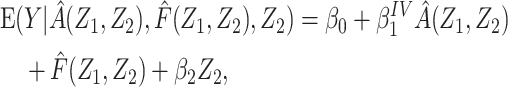
Suppose that each person in the target population has a potential outcome variable Y^a that would be observed if exposed to treatment value a. For the setting where the treatment is dichotomous, we might be interested in quantifying the population average treatment effect among the treated, .

Noting that under , if (U, Z) were observed and a standard positivity assumption held, in principle one could obtain an unconfounded estimate of the population average treatment effect or the average treatment effect among the treated using either regression-based or propensity score–based methods (11). However, in our setting adjustment for U is not feasible because U is not observed.

Typically, an investigator proceeds with analysis of the observed covariates, and might derive an estimate that controls for confounding by Z only. The resultant estimate, therefore, potentially suffers residual bias due to confounding by U, and a causal interpretation of such an estimate would require the strong (and here incorrect) assumption of no unmeasured confounding (i.e., ). How much, if any, bias due to confounding by U does a given estimate suffer? Below, we propose an empirical approach to address that question.

Proposed method

Reference population.

The proposed method requires that one has observed a reference population that as a result of a “hypothetical external intervention” a priori lacked the opportunity for exposure to A and is therefore unexposed. Let R = 1 denote the reference population while R = 0 denotes the target population of individuals all of whom a priori had an opportunity for exposure. In the target population some individuals actualized exposure (the exposed target subpopulation), but not all individuals did (the unexposed target subpopulation). In some settings an unexposed reference population may be based on observations prior to the exposure or treatment becoming available. For example, in pharmacoepidemiology, if the treatment of interest has emerged recently, information prior to introduction of a new treatment may serve this purpose, and the hypothetical external intervention preventing the opportunity for exposure is calendar time. In other settings, an unexposed reference population may arise from spatial or physical considerations that define the hypothetical external intervention preventing exposure. For example, we shall consider below the causal effect of the prompt radiation exposure from the atomic bombings of Hiroshima and Nagasaki on mortality. In the target population of residents of Hiroshima and Nagasaki who were in the cities at the time of the bombing, radiation exposure was determined by distance from ground zero and shielding; an external reference group was assembled of residents who were away from the cities at the time of the bombings (12). In the unexposed reference sample covariates, Z, and outcome, Y, are observed. Note that, as will be formalized later, we do not a priori assume that the target and reference populations are necessarily random samples from a common underlying super-population; however, we will require that a certain key population characteristic remain invariant across reference and target populations. Furthermore, throughout we assume that a standard positivity assumption holds in the treated target subpopulation, so that every treated person had, prior to being treated, a nonnegligible opportunity not to be treated.

Prognostic score.

Let F(Z) denote the expected value of Y conditional on Z among individuals in the reference group, E[Y|Z, R = 1]. Note that by virtue of treatment exclusion in the reference population, one has that F(Z) = E[|Z, R = 1]. We derive an estimate of F(Z) by fitting a regression of Y on Z to data for the reference group. This type of function is sometimes referred to as a prognostic score or disease risk score (13, 14). Here, we focus on the setting in which F(Z) is estimated using an external sample, or historical reference sample, that a priori lacked the opportunity for exposure to A and is therefore unexposed, an approach discussed by Hansen and others in the context of estimation of prognostic scores (15, 16).

Bespoke instrumental variable.

Using the estimated regression model coefficients, we compute for all individuals in our study population, and we likewise compute in the study population. Under conditions formalized below, one would expect that captures the dependence between the average potential outcome in the absence of exposure E[|Z, R = 0] and Z in both reference and study populations, in which case and Z can be expected to be mean independent in the study population. We leverage this conditional mean independence afforded by the prognostic function, to permit an instrumental variable (IV)-type analysis to address unmeasured confounding in the target population.

As noted above, the re-centering of variable induces the instrument-like (mean) independence property of Z with in the study sample. For this reason we refer to Z as a “bespoke” instrumental variable for control of potential confounding by U in an analysis of the association of interest. As we later formalize, this assumption essentially requires that the Z-Y association in the reference population matches the Z- association in the target population. This assumption has the key design ramification that one should take care in a choice of reference population so as to ensure its validity. As we further elaborate below, this assumption is significantly weaker than requiring that the reference and target population are fully exchangeable with respect to all factors (measured and unmeasured), and therefore are random samples from a common superpopulation.

Bespoke IV estimation under additive and multiplicative models.

Below we describe bespoke IV estimation of additive and multiplicative models by means of 2-stage regression and by means of g-estimation of a structural mean model. An additive marginal structural model (i.e., a linear model on an additive scale) is commonly assumed if the outcome, Y, is a continuous variable and one wishes to estimate the mean difference in Y per unit change in A. Although less commonly used for dichotomous outcomes, additive models also often are employed in the context of instrumental variable analyses if Y is a binary outcome variable and one aims to estimate the risk difference associated with a unit change in A (17). A multiplicative structural model may be preferred when the outcome mean can only take positive values, and also can be used for binary outcome variables.

Additive models

Two-stage regression.

A bespoke IV estimate of the mean difference in Y per unit change in A that does not suffer bias due to confounding by U can be derived by a 2-stage linear regression. First, we obtain the predicted value of A given Z, . This may be estimated by fitting a regression of A on Z in the study sample and evaluating for each cohort member. Second, noting that under an additive model and that is known based upon information external to the study population rather than (re)estimated in the regression model fitting, we fit a regression of Y on including as an offset, , where is the estimate of interest and accounts for the possibility that the baseline mean for the treatment-free potential outcome might differ between target and reference populations. Web Appendix 1 (available at https://doi.org/10.1093/aje/kwab288) provides SAS (SAS Institute Inc., Cary, North Carolina) code for a 2-stage estimation of the average effect of A on Y obtained under the assumption of additivity of effects, incorporating a prognostic function to create a bespoke IV and describes how to derive a bootstrap confidence interval for the estimate.

G-estimation of an additive structural mean model.

We also can derive an estimate of the parameter of interest using g-estimation of an additive structural mean model (18). For an additive model of the form, , g-estimation of the proposed bespoke IV estimator is done by identifying parameter estimates that result in lack of association between the instrument, Z, and , where is the estimate of interest. Web Appendix 1 provides a brief description of a g-estimation approach incorporating a prognostic function to create a bespoke IV, and SAS (SAS Institute Inc.) code, for estimation of the average effect of A on Y obtained under an additive structural nested mean model.

Multiplicative models

Two-stage regression.

For binary Y, an estimate of the difference in the log of the counterfactual outcome mean per unit change in a that does not suffer bias due to confounding by U can be derived by a 2-stage linear-logistic regression under certain conditions (see Web Appendix 2). First, we obtain the predicted value of A given Z, . This may be estimated by fitting a regression of A on Z in the study sample and calculating for each cohort member. Second, we fit a logistic regression of Y on including as an offset,

However, because the above approach applies only for rare outcomes (within levels of Z, A, and U) and under certain assumptions that require a continuous treatment (see Web Appendix 2), we recommend using g-estimation under a multiplicative structural mean model instead of 2-stage linear-logistic regression.

G-estimation of a multiplicative structural mean model.

For a multiplicative structural mean model of the form , where the estimate of interest is a ratio measure 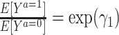, g-estimation of the proposed “bespoke” instrumental variable estimator is done by identifying parameter estimates that result in lack of association between the instrument, Z, and , where , and is the estimate of interest. Web Appendix 1 provides code for estimation of the average effect of A on Y obtained under a multiplicative structural mean model, illustrating how estimation of this model also allows us to incorporate a prognostic function to create a bespoke IV for a multiplicative structural mean model.

Partial bespoke instrumental variable.

Suppose that Z = (Z₁, Z₂) such that instead of taking all of Z as a candidate bespoke instrumental variable, we take Z₁ only as a bespoke instrumental variable, and Z₂ are additional covariates that we adjust for. In the next section, we present formal assumptions under which Z₁ is a valid candidate bespoke instrumental variable for the causal effect in view even though Z might not be. These conditions formally justify estimation methods described in previous sections by establishing sufficient identification conditions of additive and multiplicative causal effects. A simple modification to the described analytical methods can be implemented to accommodate this relaxed assumption, by further adjusting for Z₂ in the second stage regression of the proposed 2-stage regression methods. Specifically, in the second stage of 2-stage least squares under an additive model, we fit a regression of Y on and Z₂, including as an offset,

where is the estimate of interest, and is a model for , which accounts for the fact that might not be a valid bespoke instrumental variable (i.e., the risk/outcome mean under no exposure differs as a function of in target and reference populations conditional on ). Analogous adjustment applies to 2-stage linear-logistic and g-estimation of multiplicative marginal structural models previously described by further adjusting for on the logit or log scale in the outcome model respectively.

Sufficient bespoke IV identification conditions

Leveraging the instrument-like properties of Z₁, we formally establish that one can point identify , the average treatment effect among the treated given , without bias due to confounding by U, despite the fact that U is not measured (Web Appendix 2). To make identification conditions clear, suppose that Z₁ is a binary candidate bespoke instrumental variable. Identification is possible under the following conditions:

1. Consistency, such that if A = a.

2. A degenerate reference population with R = 1, in which we have =.

3. Partial population exchangeability, such that

.

4. Partial homogeneity (i.e., no interaction between A and Z₁) in causing the outcome among the treated, such that

.

5. Bespoke instrumental variable relevance: depends on z₁ for each observed z₂.

Result 1: Under conditions 1–5, we have that is uniquely identified from the empirical distribution of (Y,A,Z) in the study population and (Y,Z) in the reference population. It is in fact given by the bespoke IV estimand:

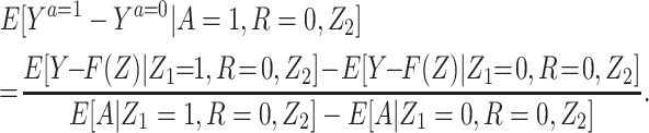A few remarks are of order regarding identification conditions for the result given above. Notably, the condition that we refer to as “partial population exchangeability” is substantially weaker than conditional population exchangeability of the target and reference populations (i.e., ), or full population exchangeability that the joint distribution of (Y^{a = 0}, Z₁, Z₂) is the same in both populations. Given consistency (condition 1) and a degenerate reference population (condition 2), “partial population exchangeability” simply requires that the Z₁-Y additive association (conditional on Z₂) in the reference population equals the Z₁-Y additive association (conditional on Z₂) among the unexposed in the study population. Note that, importantly, unlike a standard instrumental variable approach, under the proposed approach the “bespoke” instrumental variable need not be independent of U conditional on for identification purposes of the effect of treatment on the treated given . This is an additional strength of the approach relative to standard identification conditions. Finally, note that condition 4 is analogous to a no-interaction assumption routinely made in the IV setting (18, 19). This assumption clearly holds under the null hypothesis of no conditional effect of treatment in the treated and therefore the proposed approach is guaranteed to produce a valid test of the null hypothesis of no additive treatment effect provided that the remaining assumptions hold. Identification of the treatment effect on the treated under a multiplicative model is discussed in Web Appendix 2.

If we exchange the condition of “partial population exchangeability” for the stronger one of conditional population exchangeability of the target and reference populations, then we obtain some benefit. For example, in g-estimation of an additive structural mean model an estimate of the parameter may converge to 0 if the target and reference populations have comparable baseline risks (n.b., an empirically verifiable condition). If we constrain to 0 under the stronger assumption of conditional population exchangeability, this will allow for greater precision in our estimate of the parameter of primary interest, ; moreover, under this constraint we can relax the assumption of partial homogeneity (condition 4) and assess for statistical interaction between A and Z₁ in causing the outcome among the treated.

Simulation example.

Data were simulated for 1,000 studies, with 2,500 people in each study sample and 2,500 people in each unexposed reference sample. In each simulation, we generated 4 measured covariates, denoted Z₁ to Z₄, and 1 unmeasured covariate, denoted U. Z₁, Z₃, and U were random binary variables, and Z₂ and Z₄ were continuous variables assigned by sampling from a uniform (−1,1) distribution. In Web Appendix 3 we describe additional simulations where U is associated with Z. We assigned A as a random binary variable that took a value of 1 with probability 1/(1 + exp(−(−0.1 – 0.5 × Z₁ – 0.5 × Z₂ – 0.5 × Z₃ – 0.5 × Z₄ + 1 × U))); in the external reference sample, A was set to 0.

We considered 2 scenarios for the outcome variable. In the first scenario, the outcome variable, Y, was a continuous variable that took a value of (1 + 1 × Z₁ + 1 × Z₂ + 1 × Z₃ + 1 × Z₄ + 1 × U + 1 × A+ ε), where ε ~ N(0,1). In the second scenario, Y was a binary variable that took a value of 1 with probability 0.1 + 0.05 × Z₁ + 0.05 × Z₂ + 0.05 × Z₃ + 0.05 × Z₄ + 0.2 × U + 0.2 × A.

As in settings where U is unmeasured, we fitted a linear regression model to predict Y as a function of Z₁–Z₄ in the external reference sample and obtained . We used the methods described in this paper (and code in Web Appendix 1) to obtain an estimate of the average change in Y with A by a 2-stage regression, and analyses were replicated using the approach of g-estimation of an additive structural nested model.

For comparison, we fitted 2 marginal structural regression models with stabilized inverse probability of exposure weights such that exposed cohort members are given a weight defined as the ratio of the marginal probability of exposure to the estimated propensity score, while unexposed cohort members are given a weight defined as the ratio of 1 minus the marginal probability of exposure to 1 minus the estimated propensity score. In the first marginal structural model, the estimated propensity of exposure was derived from a logistic model fitted to each simulated cohort for A as a function of Z₁–Z₄. In the second marginal structural model, the estimated propensity of exposure was derived from a logistic model fitted to each simulated cohort to predict A as a function of Z₁–Z₄, and U. We summarized results from the simulated studies by computing the mean of the estimates, the estimated standard deviation of the estimates (the empirical standard error, or ESE), and the square root of the mean of squared difference between the estimated associations and the specified true effect of A on Y (the root mean squared error, or RMSE).

Web Appendix 3 reports results of additional simulations in which: 1) U was associated with Z (illustrating that, unlike a standard instrumental variable approach, the “bespoke” instrumental variable need not be independent of U conditional on ); 2) U was not associated with Y (and consequently there is not confounding by U); 3) Z was not associated with Y in the reference population (and consequently a violation of the identification condition of partial population exchangeability); 4) Z was not associated with A (and consequently a violation of the condition of bespoke instrumental variable relevance); and 5) A and Z₁ interact in causing the outcome (and consequently a violation of the condition of partial homogeneity). Additional simulations, illustrating scenarios conforming to multiplicative structural mean models with continuous and dichotomous outcomes, are also reported in Web Appendix 3.

Empirical example.

We illustrate the proposed method using empirical data that were collected as part of the Life Span Study of Japanese atomic bomb survivors. The Life Span Study includes 86,611 people who were present in Hiroshima or Nagasaki at time of bombings, were residents of the city at the time of the 1950 census, and have dose estimates based upon the DS02 dosimetry system (20). The study also includes 26,531 people who were away from the cities at the time of the bombings. The present analysis is restricted to the 8,463 survivors who were 45–49 years of age at the time of the bombings in 1945 and have been followed for vital status through December 31, 2000, of whom 1,787 were people who were away from the cities at the time of the bombings. Individual dose estimates, defined as weighted DS02 colon dose, were expressed as the weighted dose in gray (Gy) and represent the sum of the gamma-radiation dose plus the neutron dose multiplied by 10. For people who were away from the cities at the time of the bombings, DS02 colon dose estimates were set to 0 Gy. For the purposes of this example, the exposure of primary interest is defined as estimated colon dose at or above the median dose for people who were present in Hiroshima or Nagasaki at time of bombings (HIGH, 1 = at or above median; 0 = below the median); and the outcome of interest is age at death (AGEDEATH, in years). Covariates include city of residence (CITY: 1 = Hiroshima, 2 = Nagasaki) and sex (SEX: 1 = male, 2 = female). Using data for those who were away from the cities at the time of the bombings, we fitted a linear regression model for AGEDEATH as a function of CITY and SEX, and we derived an estimate of F(Z) for each study member. Next, we fitted a linear regression model for HIGH as a function of CITY and SEX, and we derived the predicted value of HIGH given the fitted model and observed covariates. A F-statistic from this (first stage) regression model is reported as a quantitative measure of the strength of association between CITY and SEX (the bespoke IVs) and HIGH (the exposure of primary interest). Then, we fitted a regression model for AGEDEATH as a function of the predicted value of HIGH, with the estimate of F(Z) as an offset term. For comparison, we fitted a linear regression model for AGEDEATH as a function of HIGH, adjusted for CITY and SEX.

RESULTS

Simulations

In simulations in which the outcome was a continuous variable (scenario 1), our proposed 2-stage regression estimator of the exposure-outcome association suffered no bias due to confounding by U, despite the fact that U is an unmeasured variable (Table 1). Equivalent results were obtained when our proposed estimator was obtained using g-estimation of an additive structural model. In contrast, estimates of association obtained from a standard marginal structural model where the propensity of exposure was derived using the observed covariates Z₁–Z₄ (but not the confounder, U) were biased relative to the simulation setup. Finally, for comparison, we derived the result that would be obtained if U was a measured covariate; we fitted a marginal structural model where the propensity of exposure was derived using the covariates Z₁–Z₄ and U and the average estimated association was unbiased. The statistical efficiency of our proposed bespoke instrumental variable estimator was lower than that of the marginal structural models fitted using inverse probability of exposure weighting (as reflected by larger empirical standard errors). The estimated root mean squared error was largest for the Z-adjusted estimate, intermediate for our proposed 2-stage regression estimator, and smallest for the marginal structural model where the propensity of exposure was derived using the observed covariates Z₁–Z₄ and the unobserved confounder U.

Table 1.

Mean Estimates, Empirical Standard Error, and Root Mean Squared Error for 1,000 Cohorts With 2,500 Observations Each^a

Scenario and Model	Estimate	ESE	RMSE
Scenario 1
Adjustment for Z	1.24	0.05	0.242
Proposed bespoke instrumental variable method	1.00	0.25	0.200
Adjustment for Z, U	1.00	0.05	0.039
Scenario 2
Adjustment for Z	0.25	0.02	0.049
Proposed bespoke instrumental variable method	0.20	0.10	0.084
Adjustment for Z, U	0.20	0.02	0.016

Abbreviations: ESE: empirical standard error; RMSE: root mean squared error.

^a Results of simulations of association between exposure, A, measured covariate, Z, unmeasured covariate, U, and binary outcome, Y.

In simulations in which the outcome was a binary variable (scenario 2), our proposed 2-stage regression estimator of the exposure-outcome association suffered no bias due to confounding by U, despite the fact that U is an unmeasured variable. Equivalent results were obtained when our proposed estimator was obtained using g-estimation of an additive structural model. In contrast, estimates of association obtained from a marginal structural model where the propensity of exposure was derived using the observed covariates Z₁–Z₄ (but not the confounder, U) were biased relative to the simulation setup. Finally, for comparison, we derived the result that would be obtained if U was observed; we fitted a marginal structural model where the propensity of exposure was derived using the covariates Z₁–Z₄ and U and the average estimated association was unbiased. The statistical efficiency of our proposed approach was lower than that of the marginal structural models fitted using inverse probability of exposure weighting (as reflected by larger empirical standard errors), and the root mean squared error of our proposed 2-stage regression estimator was greater than that of the estimates derived via the other estimators.

Web Table 1 reports simulations where U was associated with Z. Under this simulation scenario, our proposed estimator of the exposure-outcome association was unbiased, illustrating that, unlike a standard instrumental variable approach, the “bespoke” instrumental variable need not be independent of U. Web Table 1 also reports simulations that were conducted in which U was not associated with Y (and therefore was not a confounder of the association of interest). Under this simulation scenario, our proposed estimator of the exposure-outcome association was unbiased. Finally, Web Table 1 also reports simulations in which we violate the identification conditions of partial population exchangeability, bespoke instrumental variable relevance, and partial homogeneity. Under these simulation scenarios, our proposed estimator of the exposure-outcome association was biased.

Web Table 2 reports additional simulations for scenarios involving multiplicative models. Our proposed “bespoke” instrumental variable estimator of the exposure-outcome association, obtained using g-estimation, was unbiased. For comparison, we fitted a marginal structural model where the propensity of exposure was derived using the observed covariates Z₁–Z₄. The mean of the resultant estimates of association (obtained omitting the unmeasured confounder, U) was biased relative to the simulation setup. Finally, we fitted a marginal structural model where the propensity of exposure was derived using the covariates Z₁–Z₄ and U; the average estimated association conformed to the simulation set-up.

Empirical results

A regression model that included the exposure variable of interest, HIGH, adjusting for CITY and SEX, yielded an estimate of −0.31 (95% confidence interval: −0.82, 0.21), suggesting approximately 4 months of life shortening on average among the more highly exposed atomic bomb survivors aged 45–49 years at the time of the bombings (Table 2). An F-statistic derived by a linear regression model for HIGH as a function of CITY and SEX was 422.4 (2 degrees of freedom). The proposed bespoke instrumental variable estimate of the association between high estimated radiation dose and age at death was −1.76 (95% confidence interval: −3.19, −0.32) suggesting approximately 1 year and 9 months of life shortening on average among the more highly exposed atomic bomb survivors aged 45–49 years at time of bombing. The covariate, CITY, was strongly related to HIGH; 62% of Hiroshima residents were assigned a value of HIGH = 1, while 25% of Nagasaki residents were assigned a value of HIGH = 1. Unlike the simulation example, we do not know whether unmeasured confounders affect the empirical data; however, the empirical results suggest evidence for unmeasured confounding in the simple covariate-adjusted linear regression estimate.

Table 2.

Estimated Difference in Age at Death With High Radiation Dose (at or Above the Median Dose) Among Atomic Bomb Survivors Aged 45–49 Years at the Time of the Bombings, Life Span Study of Atomic Bomb Survivors, Hiroshima and Nagasaki, Japan, 1950–2000

Model	Estimate	95% CI
Adjustment for city and sex	−0.31	−0.82, 0.21
Proposed bespoke instrumental variable method	−1.76	−3.19, −0.32

Abbreviation: CI, confidence interval.

DISCUSSION

This work discusses analysis of the association between a point exposure and outcome when there is concern about residual confounding by unmeasured variables. We illustrated that a measured confounding variable can act as a “bespoke” instrumental variable in a regression analysis. This provides an approach to account for residual bias due to unmeasured confounders.

Our proposed approach requires an unexposed reference sample, which limits the utility of the proposed approach to settings in which such samples are available, similar to prior work on methods that use external/historical cohorts to estimate prognostic scores (15, 16). An unexposed reference could be defined based on historical data (if the exposure of interest has emerged recently), based on spatial considerations (e.g., if exposure is limited to a specific area or department of a study facility), or based on a contraindication for treatment (e.g., if exposure is a drug or therapy). Such examples emphasize that structural nonpositivity, rather than being a problem, here may serve to identify an unexposed reference group, which is a key design consideration for the proposed bespoke IV approach. The reference group should be external to the study sample to avoid collider bias (if Z and U are associated with A), and, if drawing upon historical data, attention should be paid to any changes in coding or recording of study data over time (13). In the context of estimation of prognostic scores using external (i.e., out-of-sample) data, Wyss et al. (21) proposed a strategy for estimation when an unexposed external reference sample was unavailable; their proposed approach made use of a sample with reduced treatment prevalence. Such an approach might be applied with our proposed bespoke IV approach if the reduced treatment prevalence was a result of a “hypothetical intervention” (e.g., limited treatment availability in an early period, or in a population outside of the target population). Importantly, the proposed approach only requires “partial population exchangeability” of the target and reference populations; this condition is substantially weaker than full exchangeability of the external reference and target populations. The target and reference populations need not have similar baseline risks of the outcome; they may differ with respect to distributions of measured and unmeasured covariates, and the association between U and Y may differ between them. “Partial population exchangeability” simply requires, given consistency and a degenerate reference population, that the Z₁-Y association in the reference population equals the Z₁-Y association among the unexposed in the target population.

The prognostic function, F(Z), captures the association between the measured covariate, Z, and the treatment-free potential outcome, . In principle, F(Z) may be estimated under any model form, such as a logistic model under which some of the problems of estimation of an additive risk model are ameliorated; however, in practice, if the model for the treatment effect is on the additive scale, then we recommend that F(Z) also be modeled on that scale.

Substantial attention has been given to exposure propensity scores and disease risk scores to balance measured covariates that are potential confounders at treatment initiation (22, 23). Such approaches require the condition of no unmeasured confounding for identification of causal effects. Here, using similar information to that required for out-of-sample estimation strategies for the disease risk score (21), we propose an approach that affords superior performance because it allows for identification of causal effects without the condition of no unmeasured confounding. Consequently, our proposed approach addresses the problem of unmeasured confounding using essentially the same information that some researchers have considered in the past in the context of disease risk scores.

We focus on situations where identification is obtained under the condition of partial homogeneity of the causal effect (condition 4 in the section, Sufficient Bespoke IV Identification Conditions, i.e., no interaction between A and Z₁ in causing the outcome among the treated). We allow that the underlying model for the treatment effect may be either an additive or a multiplicative model, thereby allowing for the investigator to specify a scale upon which the assumption of no interaction holds. This condition could be replaced by alternatives, such as no interaction between A and Z₁ in the model for selection bias due to confounding (24). The proposed method allows for a nonparametric test of the null for the causal effect of the exposure, and, under the null, the identifying condition of partial homogeneity of the causal effect holds by definition. Our empirical example illustrates the potential utility of such a test. Under a covariate conditional regression analysis, we fail to reject the null for an association between high estimated radiation dose from the atomic bomb and age at death among survivors aged 45–49 years at time of bombing; under our proposed “bespoke” instrumental variable analysis we reject the null. Under the stronger condition of full population exchangeability of the reference and target populations, we can relax some other identification conditions. For example, given full population exchangeability, we can relax the condition of partial homogeneity of the causal effect and allow for identification of interactions between A and Z₁ in causing the outcome among the treated. Alternatively, given full population exchangeability, we may relax the condition of bespoke instrumental variable relevance (condition 5 in section, Sufficient Bespoke IV Identification Conditions) and identify the average treatment effect among the treated regardless of the association between Z₁ and A.

The proposed approach works best when one has a strong “bespoke” instrument, as the proposed approach often carries a substantial cost in terms of statistical efficiency. The estimate obtained by the proposed approach may be unbiased but of relatively poor precision such that the mean square error of the proposed approach exceeds that of an estimate derived from an outcome regression model that suffered some residual confounding. One appealing aspect of the proposed approach is that an investigator may choose a strong “bespoke” instrument (or instruments) from among a set of measured covariates, Z. Furthermore, a correct but imprecise estimate is sometimes better than an incorrect but precise estimate, especially when additional data are forthcoming or possible. Standard regression diagnostics for how well Z correlates with Y, and how well Z predicts A, can provide some guidance to practitioners regarding whether they can expect stable estimates with this method; for example, as in standard instrumental variable analyses, an F-statistic from the first-stage regression can serve as a measure of whether a proposed (bespoke) instrument is associated with treatment A (25, 26).

We described a 2-stage regression approach to estimation as well as g-estimation of a marginal structural nested mean model. The former may be appealing as a simple approach for implementation for those not used to g-estimation methods. However, for a multiplicative model, the g-estimation approach is recommended, and Web Appendix 1 provides relatively simple code for its implementation. For analyses of dichotomous outcomes, we describe both additive and multiplicative models; this provides flexibility with regard to estimands and model assumptions (including the condition of partial homogeneity).

The proposed approach shares some similarity to other strategies to address residual confounding by unmeasured variables, such as the approaches of fixed-effect regression, difference-in-difference analysis, and analyses that leverage negative controls. In a fixed-effect regression, individuals are compared over time, and changes in exposure status and outcome within subjects are examined; unlike a fixed-effect model, our proposed approach allows for study of nonrecurring outcomes (we do not need to observe the outcome before and after exposure for each person) and is employed in settings of time-invariant exposures. In a difference-in-difference analysis, changes in exposure status that result from policy changes or other external factors are examined in relation to outcomes; unlike a difference-in-difference analysis, the proposed approach does not require the conditions of “natural experiment” in which an external factor leads to changes exposure status, nor does it require that we have the ability to assign pretreatment subjects to “exposed” and “unexposed” groups based on their future treatment status. While the proposed approach involves an external unexposed reference, it is only used to estimate the baseline association between observed covariates and outcome. In an analysis that leverages a negative control outcome, a secondary outcome is identified that is not directly influenced by exposure but is influenced by the observed and unobserved confounders of the exposure-outcome association of interest; unlike such an investigation, the proposed approach does not require identification of an outcome that meets the condition of a negative control. Alternatively, in an analysis that leverages a negative control population (e.g., a population in which alcohol consumption is absent), a secondary factor such as alcohol-metabolism–related genetic variants may be identified to show that in populations that generally drink no alcohol the variant has no effect on cardiovascular disease; however, such examples may be closer to demonstrating the exclusion restriction condition needed when a genetic variant is considered as an instrumental variable. Our approach, which does not require any null effects, completely relaxes exclusion restriction conditions and, more generally, provides an approach to instrumental variable–like analysis in which key identification conditions are exchanged for design considerations about a reference population. In this way, the proposed approach fills a gap for a unique set of problems that may be difficult to address using those other research designs to address concerns about unmeasured confounders.

The proposed approach may complement a standard IV analysis. When a true instrumental variable is available, one can anchor study results at the standard IV estimate and subsequently leverage our proposed bespoke IV to validate the standard IV assumptions of exclusion restriction and IV independence. Our proposed method also can help avoid problems of imprecision and bias that may arise in a standard IV analysis given a weak instrument (25) by allowing an investigator to leverage both the standard (true) instrumental variable and a strong “bespoke” instrument (or instruments) from among a set of measured covariates, Z.

Our empirical example illustrates implementation of the method in a subgroup drawn from a landmark cohort study of Japanese atomic bomb survivors. At the outset of the Life Span Study, it was recognized that the ex post facto survey lacked the conditions for rigorous causal inference afforded by randomization to treatment (12, 27), and, as one method to aid with investigation of potential biases, individuals not in the cities at the time of bombings were enrolled in the study. We note that the example is illustrative of the utility of such external reference groups, but we caution against overinterpretation of the empirical results for the small sample of data analyzed and note that a causal interpretation requires that the identification conditions enumerated in the text hold and correct model specification.

Confounding is a routine concern in observational studies. We have proposed a novel approach to assess, and account for, bias due residual confounding. The focus in the present work has been a point exposure; we have not attempted to address here the more complex problems that arise in settings of time-varying exposures, instruments, and confounders (18). For the setting in which we wish to assess potential confounding by unmeasured variables of the effect of a point exposure, the approach involves different assumptions from those typically employed and therefore may offer a useful tool.

REFERENCES

- 1. Bross ID. Spurious effects from an extraneous variable. J Chronic Dis. 1966;19(6):637–647. [DOI] [PubMed] [Google Scholar]
- 2. Gail MH, Wacholder S, Lubin JH. Indirect corrections for confounding under multiplicative and additive risk models. Am J Ind Med. 1988;13(1):119–130. [DOI] [PubMed] [Google Scholar]
- 3. Savitz DA. Interpreting Epidemiologic Evidence: Strategies for Study Design and Analysis. Oxford, UK: Oxford University Press; 2003. [Google Scholar]
- 4. Robins J, Morgenstern H. The foundations of confounding in epidemiology. Comput Math Applic. 1987;14:869–916. [Google Scholar]
- 5. Rothman K, Greenland S. Modern Epidemiology. 2nd ed. Philadelphia, PA: Lippincott Williams & Wilkins; 1998. [Google Scholar]
- 6. D'Agostino RB Jr. Propensity score methods for bias reduction in the comparison of a treatment to a non-randomized control group. Stat Med. 1998;17(19):2265–2281. [DOI] [PubMed] [Google Scholar]
- 7. Cusson A, Infante-Rivard C. Bias factor, maximum bias and the E-value: insight and extended applications. Int J Epidemiol. 2020;49(5):1509–1516. [DOI] [PubMed] [Google Scholar]
- 8. VanderWeele TJ, Ding P. Sensitivity analysis in observational research: introducing the E-value. Ann Intern Med. 2017;167(4):268–274. [DOI] [PubMed] [Google Scholar]
- 9. Lash TL, Fink AK. Semi-automated sensitivity analysis to assess systematic errors in observational data. Epidemiology. 2003;14(4):451–458. [DOI] [PubMed] [Google Scholar]
- 10. Richardson DB, Laurier D, Schubauer-Berigan MK, et al. Assessment and indirect adjustment for confounding by smoking in cohort studies using relative hazards models. Am J Epidemiol. 2014;180(9):933–940. [DOI] [PMC free article] [PubMed] [Google Scholar]
- 11. Sato T, Matsuyama Y. Marginal structural models as a tool for standardization. Epidemiology. 2003;14(6):680–686. [DOI] [PubMed] [Google Scholar]
- 12. Beebe GW, Ishida M, Jablon S. Studies of the mortality of A-bomb survivors, 1. Plan of study and mortality in the medical subsample (selection 1), 1950–1958. Radiation Res. 1962;16(3):253–280. [PubMed] [Google Scholar]
- 13. Glynn RJ, Gagne JJ, Schneeweiss S. Role of disease risk scores in comparative effectiveness research with emerging therapies. Pharmacoepidemiol Drug Saf. 2012;21(Suppl 2):138–147. [DOI] [PMC free article] [PubMed] [Google Scholar]
- 14. Richardson DB, Keil AP, Kinlaw AC, et al. Marginal structural models for risk or prevalence ratios for a point exposure using a disease risk score. Am J Epidemiol. 2019;188(5):960–966. [DOI] [PMC free article] [PubMed] [Google Scholar]
- 15. Hansen BB. The prognostic analogue of the propensity score. Biometrika. 2008;95(2):481–488. [Google Scholar]
- 16. Desai RJ, Glynn RJ, Wang S, et al. Performance of disease risk score matching in nested case-control studies: a simulation study. Am J Epidemiol. 2016;183(10):949–957. [DOI] [PubMed] [Google Scholar]
- 17. Brookhart MA, Wang PS, Solomon DH, et al. Evaluating short-term drug effects using a physician-specific prescribing preference as an instrumental variable. Epidemiology. 2006;17(3):268–275. [DOI] [PMC free article] [PubMed] [Google Scholar]
- 18. Hernan MA, Robins JM. Instruments for causal inference: an epidemiologist's dream. Epidemiology. 2006;17(4):360–372. [DOI] [PubMed] [Google Scholar]
- 19. Robins J. Correcting for non-compliance in randomized trials using structural nested mean models. Commun Stat. 1994;23:2379–2412. [Google Scholar]
- 20. Preston DL, Pierce DA, Shimizu Y, et al. Effect of recent changes in atomic bomb survivor dosimetry on cancer mortality risk estimates. Radiat Res. 2004;162(4):377–389. [DOI] [PubMed] [Google Scholar]
- 21. Wyss R, Lunt M, Brookhart MA, et al. Reducing bias amplification in the presence of unmeasured confounding through out-of-sample estimation strategies for the disease risk score. J Causal Inference. 2014;2(2):131–146. [DOI] [PMC free article] [PubMed] [Google Scholar]
- 22. Leacy FP, Stuart EA. On the joint use of propensity and prognostic scores in estimation of the average treatment effect on the treated: a simulation study. Stat Med. 2014;33(20):3488–3508. [DOI] [PMC free article] [PubMed] [Google Scholar]
- 23. Hernán MA, Robins JM. Estimating causal effects from epidemiological data. J Epidemiol Community Health. 2006;60(7):578–586. [DOI] [PMC free article] [PubMed] [Google Scholar]
- 24. Tchetgen Tchetgen E, Vansteelandt S. Alternative Identification and Inference for the Effect of Treatment on the Treated With an Instrumental Variable. Harvard University Biostatistics. Working Paper Series, No. 166. 2013. https://biostats.bepress.com/harvardbiostat/paper166. Accessed January 11, 2022.
- 25. Uddin MJ, Groenwold RH, Belitser SV, et al. Instrumental variable analysis in epidemiologic studies: an overview of the estimation methods. Pharm Anal Acta. 2015;6(353). [Google Scholar]
- 26. Staiger D, Stock JH. Instrumental variables regression with weak instruments. Econometrica. 1997;65(3):557–586. [Google Scholar]
- 27. Beebe GW, Ishida M, Jablon S. Life Span Study Report Number 1: Description of study mortality in the medical subsample October 1950–June 1958. Hirsohima, Japan: Atomic Bomb Casualty Commission; 1961. [Google Scholar]
Associated Data
This section collects any data citations, data availability statements, or supplementary materials included in this article.