Data Management and Network Architecture Effect on Performance Variability in Direct Attenuation Correction via Deep Learning for Cardiac SPECT: A Feasibility Study

Abstract

Attenuation correction (AC) is important for accurate interpretation of SPECT myocardial perfusion imaging (MPI). However, it is challenging to perform AC in dedicated cardiac systems not equipped with a transmission imaging capability. Previously, we demonstrated the feasibility of generating attenuation-corrected SPECT images using a deep learning technique (SPECT_DL) directly from non-corrected images (SPECT_NC). However, we observed performance variability across patients which is an important factor for clinical translation of the technique. In this study, we investigate the feasibility of overcoming the performance variability across patients for the direct AC in SPECT MPI by proposing to develop an advanced network and a data management strategy. To investigate, we compared the accuracy of the SPECT_DL for the conventional U-Net and Wasserstein cycle GAN (WCycleGAN) networks. To manage the training data, clustering was applied to a representation of data in the lower-dimensional space, and the training data were chosen based on the similarity of data in this space. Quantitative analysis demonstrated that DL model with an advanced network improves the global performance for the AC task with the limited data. However, the regional results were not improved. The proposed data management strategy demonstrated that the clustered training has potential benefit for effective training.

I. Introduction

SINGLE photon computed tomography (SPECT) is a tomographic noninvasive imaging modality and a clinically valuable tool for studying the function of underlying organs or tissues. Patients are injected with gamma-emitting radioisotopes and the emitted gamma rays captured by the gamma camera can show amounts of blood flow in the capillaries of the imaged region. Myocardial perfusion imaging (MPI) is one of the most common SPECT clinical applications in nuclear cardiology. SPECT MPI has a valuable efficacy in the evaluation and risk stratification of patients with known or suspected cardiovascular disease [1]. However, the diagnostic accuracy and clinical interpretation of myocardial SPECT images are often hampered by photon attenuation caused by the breasts, lateral chest walls, abdomen, and diaphragm [2]. Attenuation artifacts can adversely affect the accuracy of diagnosis and lead to unnecessary invasive angiography procedure [3]. Several studies have demonstrated that attenuation correction can improve both sensitivity and specificity for the detection of coronary artery disease (CAD) and generate a relatively uniform tracer distribution for patients with a low likelihood of CAD [4], [5], [6]. American society of nuclear cardiology and the society of nuclear medicine and molecular imaging recommend the incorporation of attenuation correction to improve the diagnostic accuracy [7].

SPECT/CT hybrid systems correct the attenuation artifacts by using attenuation maps obtained by performing an additional CT scan. However, the hybrid systems are more expensive than stand-alone SPECT systems and increase patients’ radiation dose due to performing the extra CT scan. Furthermore, the respiratory and cardiac motion may cause incorrect attenuation correction artifacts due to a mismatch between SPECT and CT data in the hybrid systems. Meanwhile, stand-alone SPECT systems which are not equipped with an external CT source currently occupy the majority (80%) of cardiac SPECT market share [8]. Therefore, correcting the attenuation without generating the attenuation maps as an intermediate step is important, especially in stand-alone SPECT systems. As we demonstrated in our previous study, it is feasible to use a deep learning approach to correct the attenuation in the image domain by using only non-corrected SPECT images, which is distinct from conventional approaches using CT data or generating pseudo-CT data as an intermediate step [9].

Recently, deep learning has become an active area of research in different medical imaging applications because of its unprecedented success in various computer vision tasks [10], [11]. However, despite all the efforts and enthusiasm, deep learning models are rarely translated into clinical care and the evidence of clinical impact remains limited [12]. Accuracy and stability are both important for developing reliable numerical algorithms. Deep learning algorithms usually have not been subject to the same rigorous standards as the traditional algorithms and stability examination is usually absent in most current deep learning-based algorithms [13], [14].

Instability is a well-established problem in some computer vision tasks such as image classification. The high performance of many deep learning methods for image classification comes at the cost of instability. A small perturbation in training data used to build the model can result in models with different generalization accuracy [15], [16], [17], [18]. Deep learning for image reconstruction as an inverse problem can also suffer from different forms of instabilities which often are independent of the underlying mathematical model. Perturbation in the image domain, structural changes, and changes in the number of samples can potentially cause different forms of instability in the result of the reconstructed images [13]. Neural networks (NN) trained with small datasets also often exhibit an unstable behavior in their performance, which leads to limit both reproducibility and objective comparison between different designs [19]. K-fold cross-validation and ensemble learning are approaches that attempted to address the stability problem caused by small training data in NNs [20]. Therefore, instability is not a rare phenomenon, and finding effective remedies is an important task to pave a path towards deep learning clinical translation.

Similar to SPECT, AC is an important step in positron emission tomography (PET) for generating quantitatively reliable and accurate images. Several studies have been proposed to improve AC in PET images using deep learning approaches [21]. For PET/MRI, deep neural networks are employed for the conversion of MR images to a pseudo-CT or attenuation map [21], [22], [23], [24]. Alternative approaches generate pseudo-CT or attenuation corrected images directly from non-corrected images [25], [26], [27], [28]. Direct deep learning conversion from non-corrected to attenuation corrected SPECT images was used in this study.

In this study, we aim to develop a strategy against the performance variability of deep learning models with limited data in the attenuation correction (AC) task. We made two hypotheses: First, deep learning models with advanced architectures and training strategy can improve the overall AC performance, compensating for the variability. To investigate, we quantitatively compared the U-Net with Wasserstein cycle generative adversarial network (WCycleGAN). CycleGAN architecture has been also studied and demonstrated accurate results for PET attenuation correction [29]; Second, a data management strategy can enable deep learning models to learn attenuation patterns more effectively and to be robust to new unseen data of which patterns are different from the patterns of training data. To investigate, we used the t-distributed stochastic neighbor embedding (t-SNE) and balanced iterative reducing and clustering using hierarchies (BIRCH) techniques. Non-corrected SPECT images (SPECT_NC) with similar distribution were placed in the proximity of one another in the low-dimensional space. Training data were chosen based on the proximity of the data in this new lower-dimensional feature space.

II. Materials and Methods

A. Data Acquisition

This retrospective stress-only myocardial perfusion SPECT study was approved by the institutional review board (IRB). 100 patients (42 female and 58 male subjects) injected with ^99mTc-tetrofosmin were scanned on GE Discovery NM/CT 570c SPECT/CT scanner at Yale New Haven Hospital. Corresponding CT data for each subject was acquired with the parameters of 120 kV p, 50 mA, and rotation time of 0.4 s. GE Attenuation Correction Quality Control (GE ACQC) package was used to correct the attenuation by the rigid alignment of CT and SPECT_NC in the myocardium region. The reconstruction of images was conducted using the one-step-late algorithm with Green prior. CT based attenuation corrected images (SPECT_CTAC) were reconstructed with 60 iterations and post-filtered by Butterworth filter with a cutoff of 0.37 cm¹ and an order of 7 and will be used as the ground truth data. SPECT_NC images were reconstructed with 30 iterations and post-filtered by Butterworth filter with a cutoff of 0.4 cm⁻¹ and an order of 10. All reconstruction parameters are clinically used at Yale New Haven Hospital. To enable easy up-sampling and down-sampling of data through our networks’ architecture, the original size of reconstructed images (70 × 70 × 50 with an isotropic voxel size of 4mm × 4mm × 4mm) was changed to 64 × 64 × 32 to enable down sampling by removing edges from the images. Moreover, voxel values were normalized to a scale of 0 to 1 by the maximum value of volumetric images.

B. Deep Convolutional Neural Network (DCNN): Architecture and Training

The first hypothesis is that an advanced network architecture can reduce the overallperformance variability. To investigate, the simple U-Net, developed in our previous work [30], was compared with a generative adversarial network (WCycleGAN) [31] that is developed for this study as an advanced network. The U-Net with added residual blocks (ResUNet) was used to test the second hypothesis. These networks were trained to generate attenuation corrected images (SPECT_DL) directly from SPECT_NC in the image space, without generating μ-maps as an intermediate step.

1). Residual U-Net (ResUNet):

The U-Net model developed in our previous study [30] was a U-Net-like model [32] which was repurposed and developed for the image-to-image translation task. Our ResUNet architecture is also a U-Net-like architecture combined with residual blocks. The ResUNet consists of 4 contracting (encoder) paths and 4 expansive paths (decoder) with symmetry concatenate connections (skip connections) between corresponding stages of the encoder and decoder. The encode-decoder structure can extract multiscale features at different resolutions by progressively down-sampling and up-sampling through the encoder and the decoder’s layers respectively. The convolution operator (Conv) with a kernel size of 3 and instance normalization (IN) was used at each step of the encoder and the decoder. For activation, leaky rectified linear unit (LReLU) and ReLU were used for the encoder and the decoder, respectively (Fig. 1).

Fig. 1.

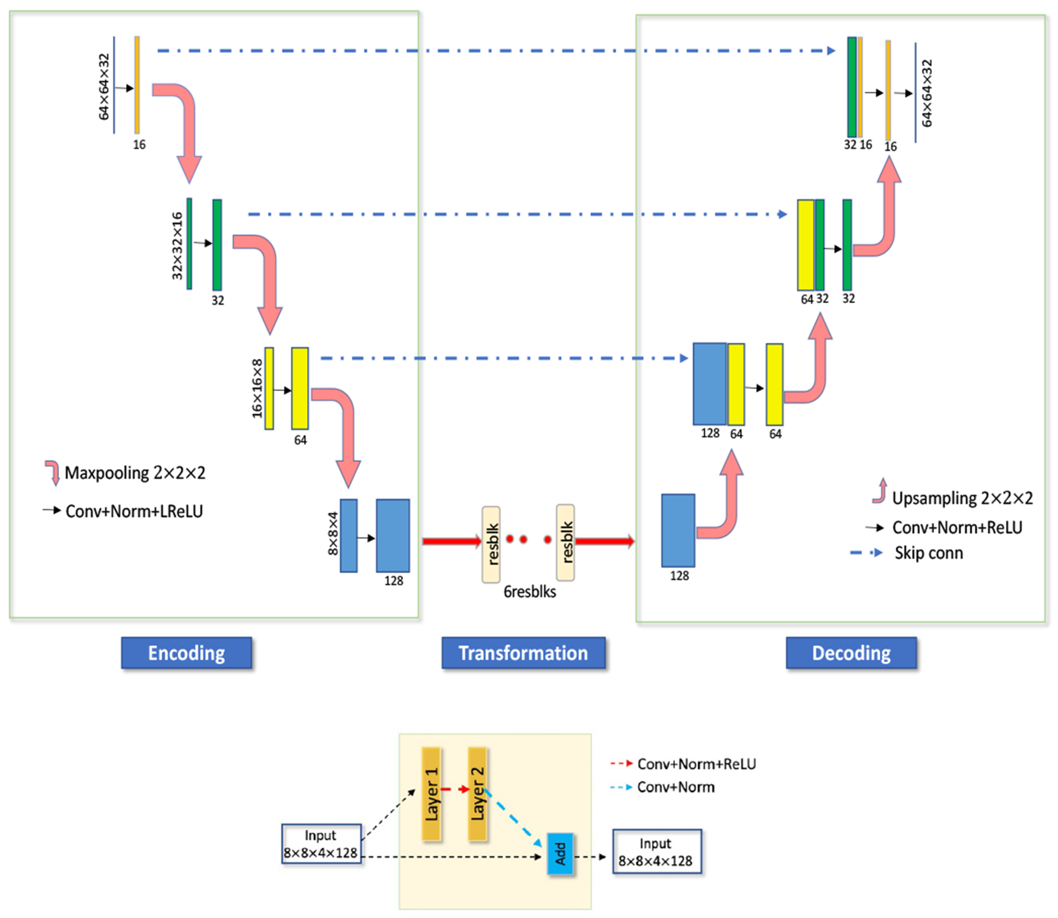
Proposed ResUNet (top) with residual blocks (bottom).

The residual blocks were embedded in the network after the last layer of the encoder. Each residual block consists of two convolution layers along with the ReLU activation function. Incorporating residual blocks into the contracting and symmetric expanding paths of the U-Net architecture mitigates the gradient vanishing problem when the network goes deeper and can further improve the performance [33].

The added skip connections can help to regain some of the lost gradient information by combining hierarchical features [34]. Moreover, it can provide a better model convergence and performance in image translation applications [34]. The overall architecture can be seen in Fig. 1.

2). Wasserstein Cycle Generative Adversarial Network:

The CycleGAN model is a generative model [35] proposed to improve the image-to-image translation task and can learn the mapping functions F : Y → X and G : X → Y between two domains X and Y [31]. The adversarial loss in this model learns the mapping such that to match the distribution of generated images to the data distribution in the target domain. The added cycle consistency loss encourages F(G(x)) ≈ x and G(F(y)) ≈ y to prevent the learned mappings G and F from contradicting each other. D_X and D_Y are two adversarial discriminators where D_X aims to distinguish between the images x and translated images G(F(y)); in the same way, D_Y aims to discriminate between the images y and G(x). Adversarial losses are applied to both mapping functions F and G. For the mapping function G : X → Y and its discriminator D_Y, the objective function is defined as:

$$\begin{gathered} L_{GAN}(G,D_Y,X,Y)=E_y[\log D_Y(y)] \\ +E_x[\log (1-D-Y(G(x)))] \\ {\mathit{min}}_G\mathit{max}{D}_Y{L}_{GAN}(G,D_Y,X,Y) \end{gathered}$$ (1)

The cycle consistency loss is defined as:

$$\begin{gathered} L_{cyc}=E_x[||F(G(x))-x||] \\ +E_y[||G(F(y))-y||] \end{gathered}$$ (2)

The identity loss enforces that the generator which is provided with images from the target domain to generate the same image without change. The identity loss is defined as:

$$L_{iden}(G)=E_x\left|\right|G(y)-y\left|\right|$$ (3)

Combing these two losses results in the following objective function:

$$\begin{gathered} L(G,F,D_X,D_Y)=L_{GAN}(G,D_Y,X,Y) \\ +L_{GAN}(F,D_X,Y,X) \\ +{\lambda }_1{L}_{cyc}(G,F) \\ +{\lambda }_2{L}_{iden}(G) \\ +{\lambda }_3{E}_x\left|\right|G(x)-y\left|\right| \end{gathered}$$ (4)

where λ₁, λ₂ and λ₃ controls the relative importance of the two objectives. and The last term is an additional estimation of error loss which we added to the main objective function to make sure that the generated images are similar to the real attenuation corrected images. The aim is to solve:

$$G*,F*={\mathit{argmin}}_{G,F}{\mathit{max}}_{D_X,D_Y}L(G,F,D_X,D_Y)$$ (5)

The CycleGAN was first proposed for unpaired image-to-image transition task [35]. In our case we have access to paired non-corrected and corrected data, and we revised the network based on our application. The network was trained with paired non-corrected and attenuation corrected data.

Although GAN models have been successful in different generative tasks, training a GAN model is challenging due to finding and maintaining an equilibrium between the capabilities of the generator and discriminator. The Wasserstein GAN model addressed this problem by introducing the Wasserstein distance as a new loss function and replacing the discriminator with the critic model [36]. The Wasserstein distance that measures the similarity between two probability distributions is continuous and differentiable almost everywhere. For this reason, the Wasserstein distance is more sensible than other commonly used cost functions such as cross-entropy and least-squares loss. We customized the CycleGAN network explained above by replacing its loss function with the Wasserstein loss and used the ResUNet model as its generator to investigate whether an advanced model can reduce the overall performance variability in the AC task.

The number of trainable parameters for U-Net and WCycleGAN are about 6 million and 17 million respectively.

3). Training:

The models were trained and tested based on paired SPECT_NC as input and corresponding SPECT_CTAC as output by using the leave-one-subject-out cross-validation (LOSO-CV) procedure. Hyperparameters such as a learning rate were empirically chosen by tuning the network. The learning rate for ResUNet was initialized to 0.0002 and reduced to zero after 100 epochs. The initial random weights of layers were selected randomly from a normal distribution. Mean squared error (or L2 loss) and RMSprop optimizer [37] were used for optimizing the weights.

In the CycleGAN model training, the generator and discriminator were trained in an alternative manner [35]. The networks were trained with a learning rate of 0.0001 for both the generator and the discriminator. The learning rate was set to 0.0002 for the first 100 epochs and linearly decayed to zero afterward. Layers’ weights were initialized as above. The Wasserstein distance and RMSprop optimizer were used for optimization.

C. Hierarchical Clustering of Data in the t-SNE Space

We investigated whether data management can reduce performance variability through subgroup-based training by using the t-SNE technique that enables hierarchical clustering of SPECT data in a low dimension of polar plots. The t-SNE is a nonlinear statistical method for dimensionality reduction and visualizing high-dimensional data by embedding the data into a low-dimensional space of two or three dimensions suitable for human observation [38].The t-SNE preserves the local structure of the data by first computing a probability distribution which is proportional to similarity of data pairs in a high-dimensional space. Then, it defines a similar probability distribution using the student t-distribution over data in low-dimensional space. Finally, it learns the dimensionality reduction map that reflects the similarities between the high-dimensional inputs by minimizing the Kullback–Leibler divergence (KL divergence) between the two distributions using a gradient descent approach.

For hierarchical clustering, the t-SNE algorithm was applied on 17-segments polar plots of SPECT_NC with the following parameters: 4 principal components, 4000 iterations, and 30 exaggeration. One of the critical parameters for the t-SNE is perplexity (exaggeration) which reflects the number of nearest neighbors that are used in the algorithm and usually have values between 5 and 50. Larger datasets usually require a larger perplexity. The perplexity parameter in this study was set to 30. Number of principal components can be set empirically or using a method explained in Appendix V. Other hyperparameters were set as the algorithm’s default values. Consequently, the dimensional of the data was reduced from 17-dimension to 2.

We are interested in clustering of the data based on attenuation pattern which is better viewed in the polar maps. In addition, the size of dataset (100) is much smaller than the whole SPECT dimension which makes the dimensionality reduction difficult and not accurate. The polar maps in this study were only used for clustering and analysis.

We assume that data with similar polar-map patterns tend to be in proximity of each other in the t-SNE space. For data management, data points in the t-SNE space were clustered into three groups by utilizing the BIRCH clustering algorithm [39]. BIRCH is an unsupervised clustering algorithm that first summarizes the data into smaller and dense regions called clustering feature entries (CF). Then applies an existing clustering algorithm like k-means directly to the sub-clusters represented by their CF vector. Here we used BIRCH combined with the k-means to cluster the data in the t-SNE space into three groups.

D. Quantitative Analysis

The normalized root mean square error (NRMSE), the peak signal-to-noise ratio (PSNR), and the structural similarity (SSIM) were used to evaluate the quantitative accuracy of the SPECT_DL compared with CT-based attenuation corrected images (SPECT_CTAC) at the voxel-wise level. Lower NRMSE and higher SSIM and PSNR indicate better similarity. The evaluation measurements are defined as below:

$$NRMSE=\sqrt{\frac{{\sum }_{i\in V}{((I)(i)-I_{ref}(i))}^2}{{\sum }_{i\in V}{I}_{ref}(i){)}^2}}$$ (6)

$$PSNR=10{\log }_{10}(\frac{N.{\mathit{max}}_{i\in V}I(i),I_{ref}(i))}{{\sum }_{i\in V}{(I(i)-I_{ref}(i))}^2})$$ (7)

$$SSIM=\frac{(2\mu {\mu }_{ref}+c_1)(2+{\sigma }_{ref}+c_2)}{({\mu }^2+{\mu }_{ref}^2+c_1)({\sigma }^2+{\sigma }_{ref}^2+c_2)}$$ (8)

where V is image volume. I is either SPECT_NC or SPECT_DL, and I_ref is SPECT_CTAC. μ, and σ denote the mean and variance of the image I. c₁ and c₂ are variables for stabilizing the division with a weak denominator.

Joint histograms were also used to show the statistical distribution of voxel-by-voxel correlation with the reference. Polar maps were utilized to evaluate the regional accuracy quantitatively.

Based on American Heart Association recommendation, the muscle and cavity of the left ventricle can be divided into 17 segments which generates three circular sections of the left ventricle named basal, mid-cavity, and apical. Fig. 2b shows the 17-segment model. With the recognition of the anatomic variability, the individual segments may be assigned to specific coronary artery territories as follows: Left Anterior Descending (LAD) that includes segments 1, 2, 7, 8, 13, 14, and 17; Right Coronary Artery (RCA) that includes segments 3, 4, 9, 10, and 15; Left Circumflex (LCX) that includes segments 5, 6, 11, 12, and 16.

Fig. 2.

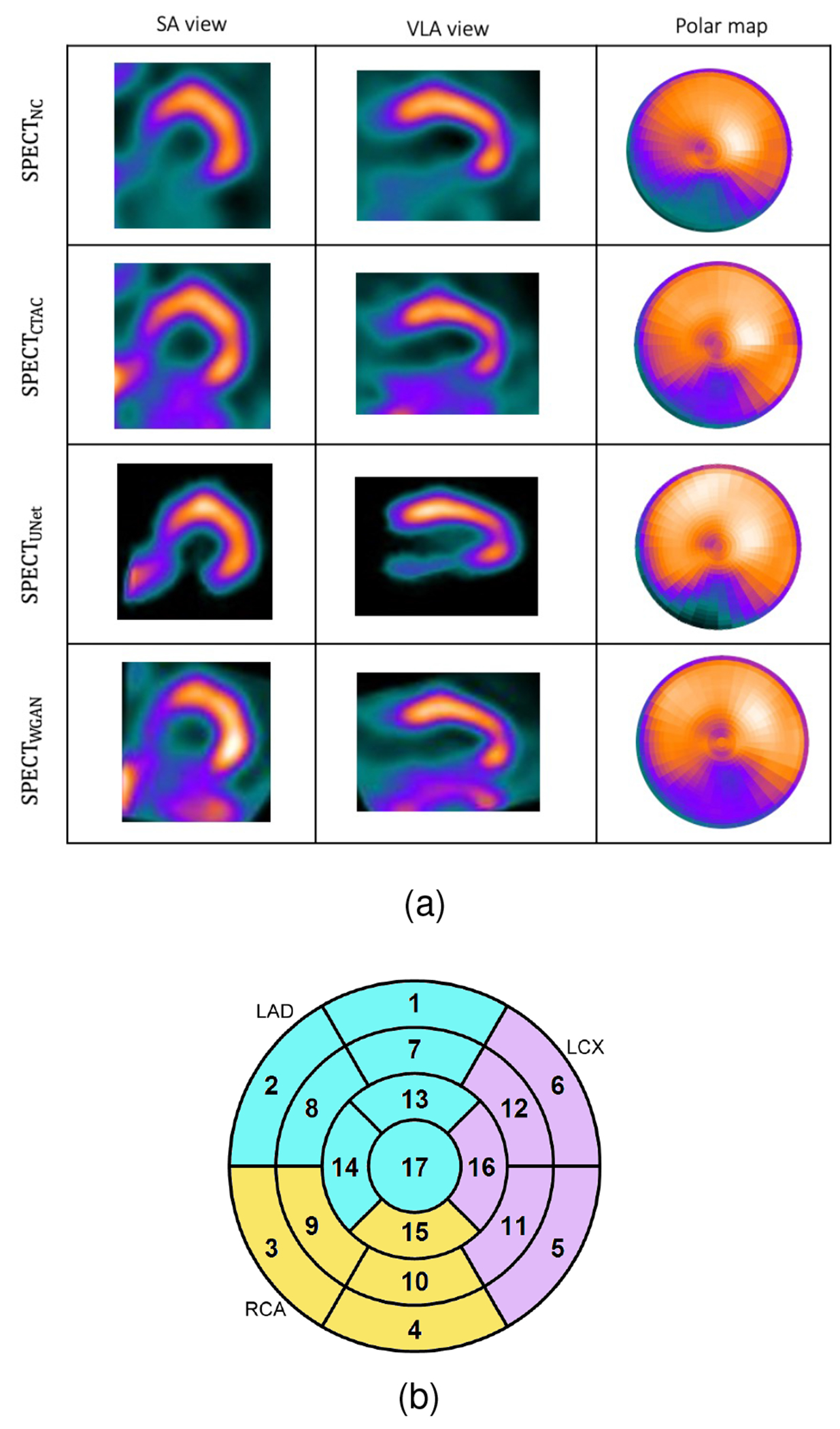
(a): Visualization of the results of the trained network on a sample patient which WCycleGAN outperform. (b): Cardiac 17 segments standard model.

The 17-segment model of the left ventricle was computed from the generated polar maps and used for the regional analysis. The error distribution of the three clusters in comparison with three random sets were displayed in box plots. A paired t-test was performed for comparing the segmental uptake values. A p-value of less than 0.05 indicates statistical significance.

III. Results

A. Impact of DL Architecture on AC Task

Our first hypothesis is that the WCycleGAN as an advanced network can reduce the performance variability of the simple U-Net. In Table I, the WCycleGAN improved the quantitative results compared with the U-Net. All the p-values are less than 0.001 which implies that the results are statistically significant. Compared with SPECT_U-Net, SEPCT_WCycleGAN improved the NRMSE by 8.9%.

TABLE I.

Voxel-wise analysis for different deep learning models. The NRMSE, PSNR, SSIM compared to the reference SPECT_CTAC (mean ± SD).

	NRMSE	PSNR	SSIM
NC	0.226 ± 0.078	31.771 ± 2.996	0.988 ± 0.007
U-Net	0.148 ± 0.095	36.2 ± 4.1	0.993 ± 0.006
WGAN	0.135 ± 0.064	36.615 ± 3.45	0.995 ± 0.004

In our previous development of the U-Net (SPECT_U-Net), low-count voxels outside of the myocardium were considered background noise and removed by binary masking as an optional preprocessing step to improve the results [30]. Consequently, the right ventricle was unseen in the SPECT_DL. One of the benefits of using WCycleGAN is that it can perform well without removing the low counts voxels outside of the myocardium as the background noise from input patches. Physicians often prefer to look at the whole image including the areas outside the myocardium. Fig. 2 shows the visualizations of images and polar maps from a sample patient which U-Net fails to perform well. The large difference between the two methods can be seen in the polar map RCA region.

The joint histograms in Fig. 4 demonstrate the voxel-wise correlations with SPECT_CTAC for SPECT_NC (slope = 0.87; R2 = 0.81), SPECT_U-Net (slope = 0.94; R2 = 0.91), and SPECT_WCycleGAN (slope = 0.98; R2 = 0.99). The WCycleGAN improved the similarity of results to the reference SPECT_CTAC, which is consistent with the results in Table I.

Fig. 4.

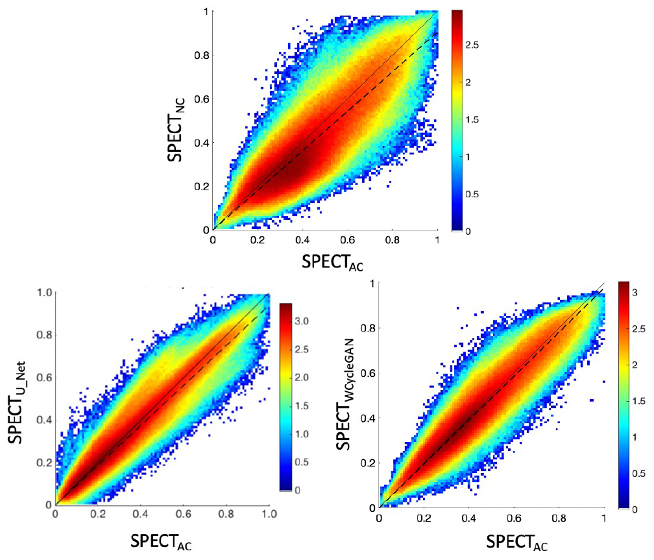
Joint histogram: (top) SPECT_NC versus SPECT_CTAC slope (dashed line) = 0.87, (bottom left) SPECT_U-NET versus SPECT_CTAC, slope = 0.94, (bottom right) SPECT_WCyCleGAN versus SPECT_CTAC, slope = 0.98. To visualize small counts in the joint histograms, the counts were log-scaled (i.e., log(counts)).

Fig. 5 shows the box plot for NRMSE across non-corrected, U-Net, and WCycleGAN. The box plot shows that the number of outliers are larger for the WCycleGAN compare to the U-Net. Fig. 6 shows the images and polar maps for a sample outlier case marked in the Fig. 5.

Fig. 5.

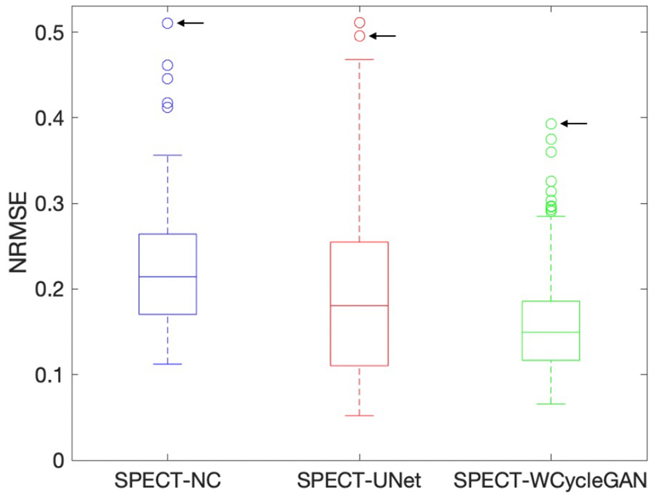
Box plots for NRMSE across non-corrected, U-Net, and WCycleGAN. The black arrow shows a shared sample outlier.

Fig. 6.

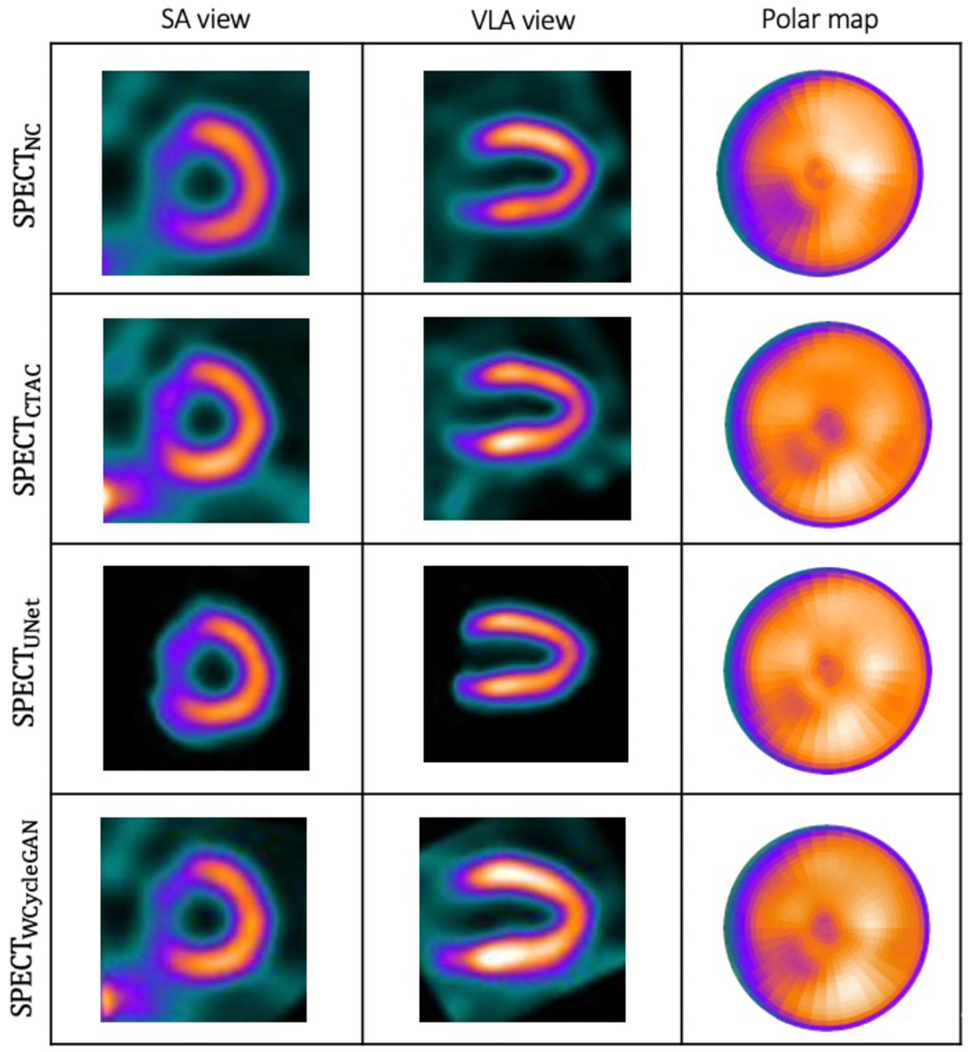
A sample outlier case shown by arrow in Fig. 5

Fig. 7 shows the distributions of segmental errors across all the subjects. Although the WCycleGAN can improve the global quantitative results, segmental errors do not improve. The average absolute segmental errors were 3.31 ± 2.87 and 5.04 ± 4.06 for SPECT_U-Net and SPECT_WCycleGAN, respectively (p < 0.001). Table II show mean and standard deviation of percentage segmental error for each segment. Fig. 3 illustrates a case which U-Net outperform the WCycleGAN.

Fig. 7.

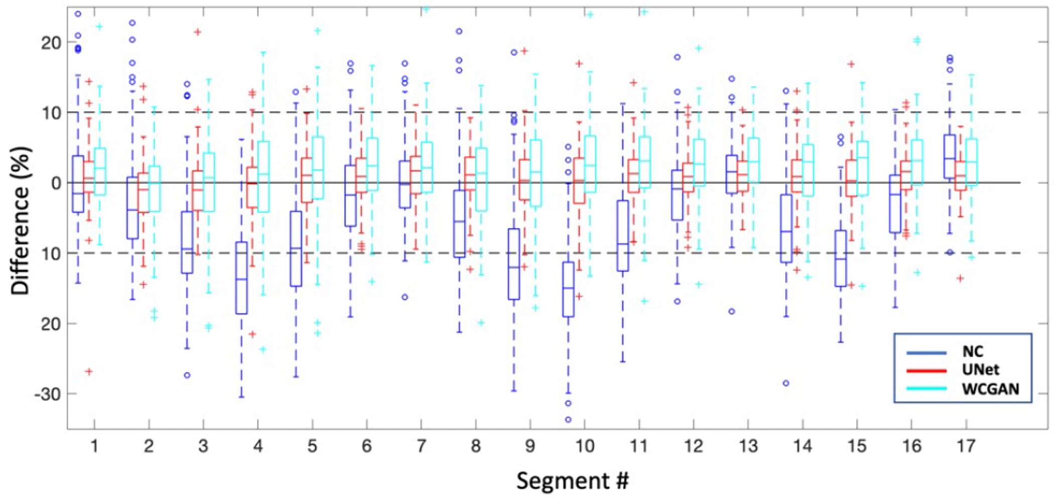
Box plots for percentage segmental errors across all the subjects

TABLE II.

mean and standard deviation of percentage segmental error for each segment (mean ± SD). Rows represent segment’s number.

	NC	UNet	GAN
1	0.06 ± 7.7	0.78 ± 4.6	1.92 ± 5.2
2	−2.37 ± 8.	−1.45 ± 4.5	−0.88 ± 5.6
3	−8.58 ± 7.6	−1.11 ± 4.7	−0.12 ± 6.8
4	−13.26 ± 7.8	−0.59 ± 5.5	0.72 ± 7.5
5	−8.88 ± 8.4	0.48 ± 4.8	2.02 ± 7.8
6	−1.78 ± 7.6	1.09 ± 4.1	2.51 ± 5.8
7	0.14 ± 6.2	1.24 ± 3.9	2.48 ± 5.5
8	−4.66 ± 7.8	1.09 ± 4.1	0.53 ± 6.3
9	−11.04 ± 8.3	0.38 ± 5.0	1.14 ± 6.7
10	−14.72 ± 7.3	−0.03 ± 5.0	2.38 ± 6.8
11	−8.21 ± 7.1	0.95 ± 4.1	2.83 ± 6.4
12	−1.52 ± 6.4	0.97 ± 3.8	2.84 ± 5.4
13	1.34 ± 5.0	1.08 ± 3.1	3.17 ± 4.6
14	−6.35 ± 6.9	0.88 ± 4.3	1.90 ± 5.7
15	−10.54 ± 6.1	0.44 ± 4.1	2.60 ± 6.2
16	−2.79 ± 6.0	1.12 ± 3.2	3.24 ± 5.2
17	3.78 ± 5.3	0.92 ± 3.5	3.11 ± 4.9

Fig. 3.

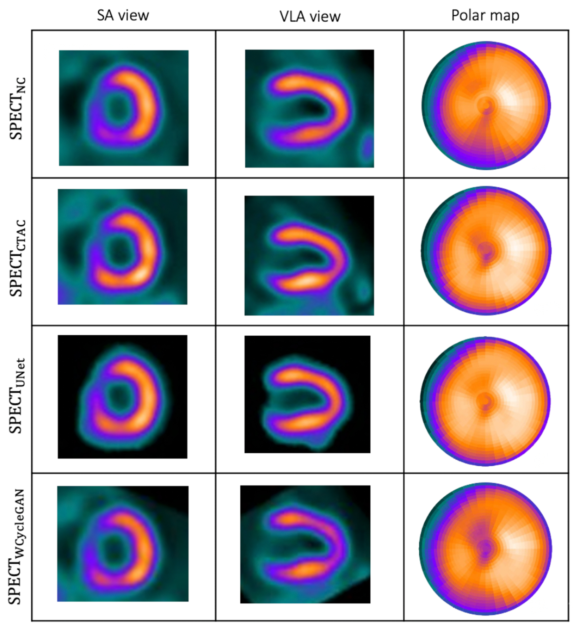
Visualization of the results of the trained network on a sample patient which U-Net outperform.

Based on the results on the limited dataset, we see that the WCycleGAN improved the results globally but not regionally, using three times more parameters. This point initiated the 2nd part where we propose a data management strategy.

B. Data Management

1). Sorting the Data in the t-SNE Space:

We hypothesized that hierarchical clustering in a low-dimensional feature space obtained by the t-SNE can reduce performance variability observed in our previous work.

Fig. 8 shows non-corrected polar plots samples picked from each group in the t-SNE space (highlighted). Noncorrected data with a similar distribution of polar plots tend to be close to each other in the t-SNE space and the proximity of data in this new space can be used as a means of clustering. Data with more uniform patterns are in group one, and groups two and three include data with nonuniform patterns.

Fig. 8.

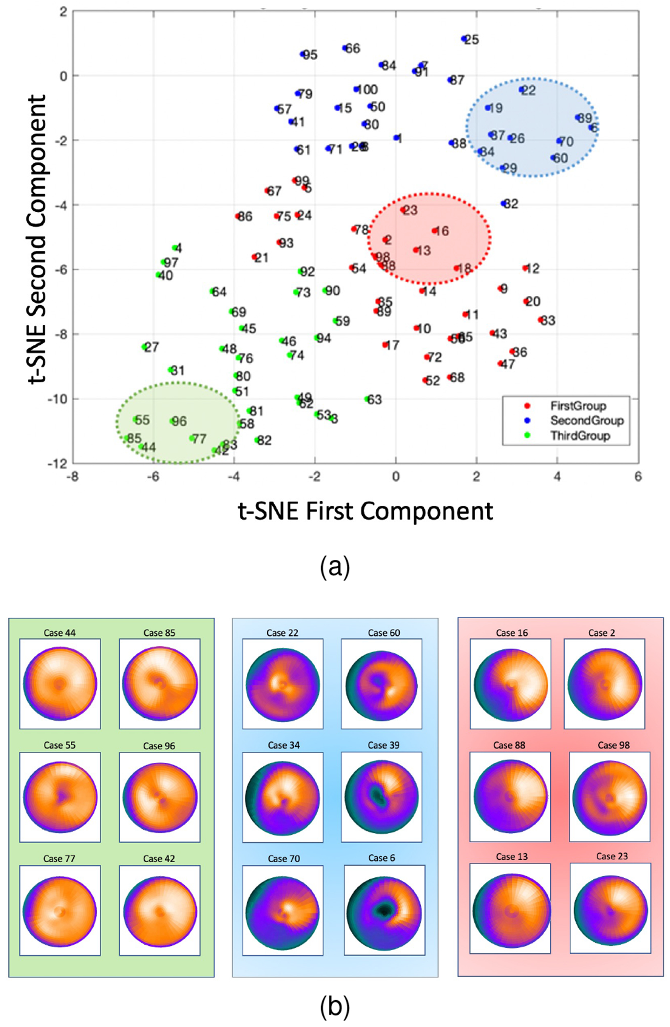
(a): 2D embedding of data in the t-SNE space, clustered into 3 groups using hierarchical clustering technique. (b): Sample data from each group highlighted in (a).

2). Clustered versus Random Training:

To explore an effect of subgroup-based training, three subgroups with the same size as the clusters were randomly selected from all 100 patches as training sets. The quantitative results of the models trained with the clusters versus models trained with the random sets were compared in Fig. 9. The p-value from paired sample t-test between NRMSE of clustered and random training are 0.01, 0.24, and 0.65 for G1, G2, and G3 respectively.

Fig. 9.

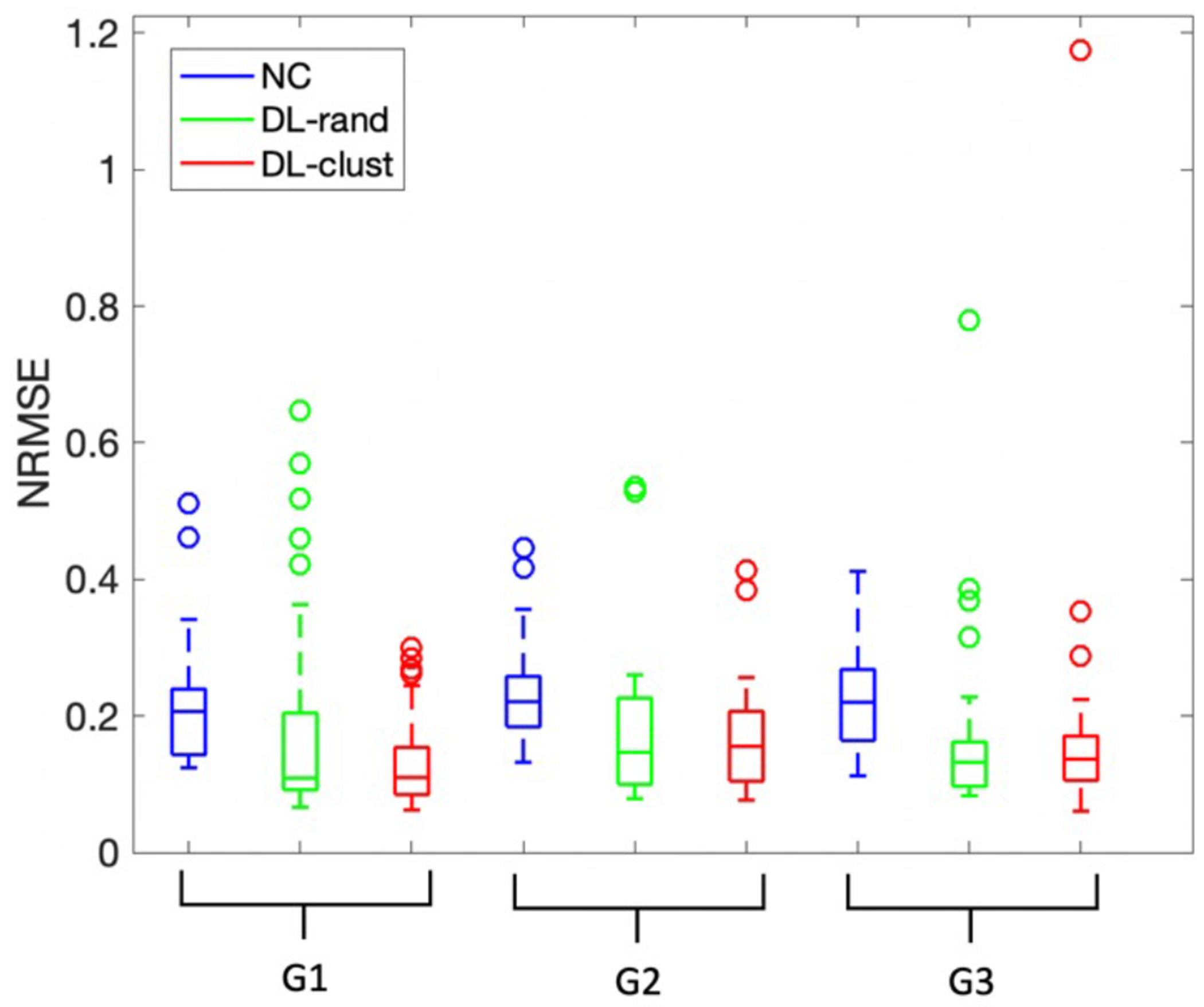
Box plots for quantitative comparison of clustered training versus training with random dataset which has same size as the clusters. SPECT_NC (blue), SPECT_DL-rand (green), and SPECT_DL-clust (red).

In Fig. 9, the performance variability is smaller for G1 and G2 when the training set is chosen from the clusters versus when the training set is randomly picked. Clustered training improved the similarity by 36.3% and 6.5% for NRMSE for G1 and G2, respectively and overall, by 12%, demonstrating the potential benefit of using cluster-based training.

The LAD artery is the largest coronary artery which provides the major blood supply to the interventricular septum. it is the most commonly occluded of the coronary arteries and its blockage due to coronary artery disease can lead to myocardial infarction and serious impairment of cardiac performance. Fig. 10 shows that clustered training reduced the average absolute error of random training by about 15% for the LAD region across subjects in group one. The average segmental errors (mean ± SD) for SPECT_rand and SPECT_clust were 3.40 ± 9.34 and 0.41 ± 10.46 respectively with p-value < 0.001 for LAD; 4.97 ± 5.1 and 3.28 ± 3.54 with p-value > 0.01 for RCA; and 1.27 ± 3.1 and 1.87 ± 7.03 with p-value > 0.1 for RCX region. Fig. 11 shows the results of the clustered training and random training for a sample case which random clustering fails to perform well. The difference between the two methods is most obvious in the LAD region.

Fig. 10.

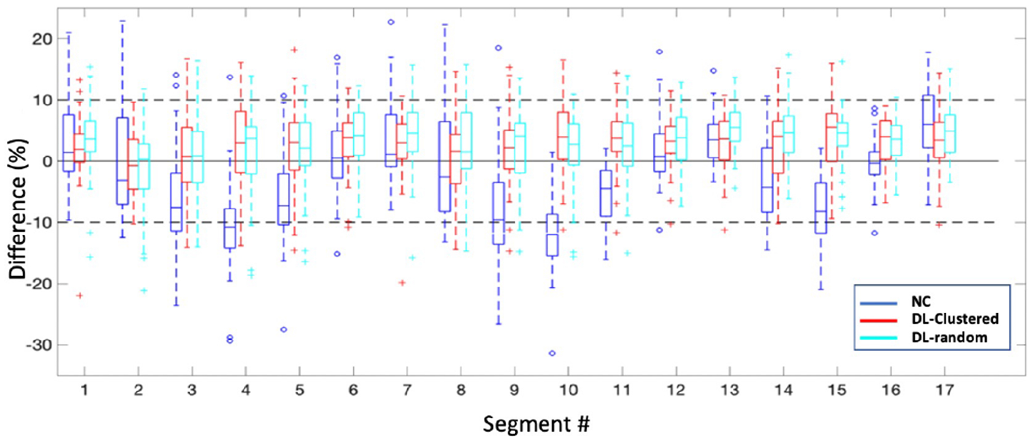
Box plots for percentage segmental errors across subjects in group 1.

Fig. 11.

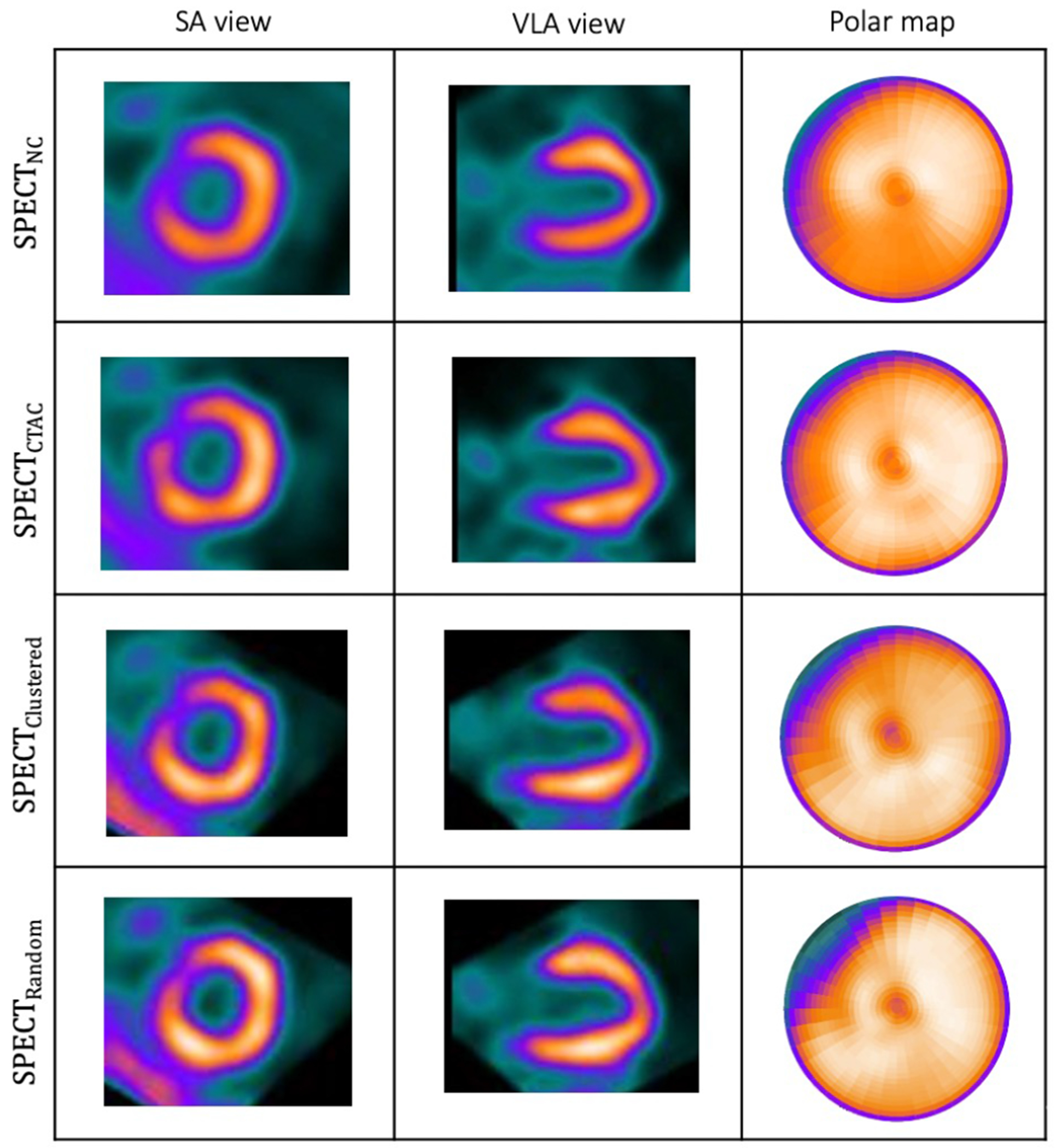
Visualization of results of clustered vs random training (sample patient).

3). Similarity of Data Distribution Between the Test and the Training Set:

We also investigated how the similarity of test data to its training set can affect the performance. To investigate, we tested each data against a model trained with the 30 closest data points to that test case and compared it with a model trained with 30 most distant data points to that test case in the t-SNE space. We used Euclidean distance and coordinates of data in the t-SNE space to measure the distance between the data points (Fig. 12). In comparison to the reference SPECT_CTAC, the NRMSE was 0.1620 ± 0.1098 and 0.1724 ± 0.1274; PSNR was 35.4050 ± 3.8512 and 34.9303 ± 3.8859; SSIM was 0.9937 ± 0.0067 and 0.9928 ± 0.0080 for using the 30 closest and the 30 farthest data for training, respectively. Using similar training data to the test set improves the results by 6.4% in terms of NRMSE (p < 0.001). This shows the potential benefit of data management for the SPECT AC task.

Fig. 12.

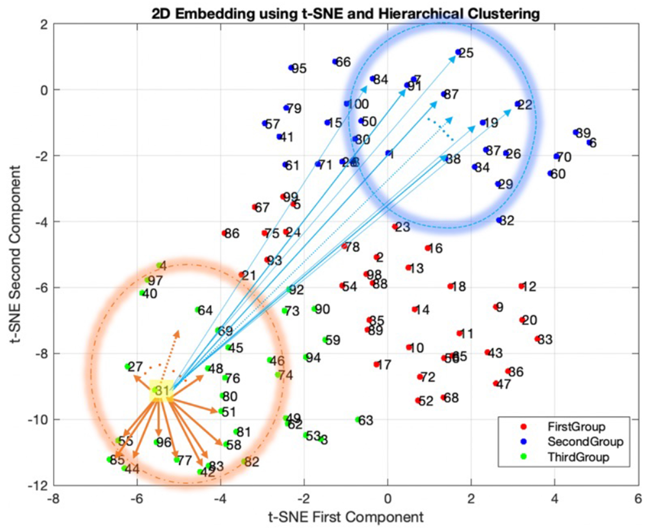
Schematic figure showing how each data point was tested against the 30 closest and 30 farthest training set in the t-SNE space.

4). Clustered versus Standard Training:

Here we compared the results of the clustered training with the standard training using all the available data. Three sub-groups were clustered as different training sets (G1,G2,G3) by the BIRCH technique in the t-SNE space. The quantitative result of each cluster (clustered training) was compared with corresponding data in the standard training using all the data. Note that each cluster contains only about 33 input patches among all 100 patches. Test results of standard training using all the data in the original space were computed and corresponding data from each cluster were picked from the test results to be compared with the clustered training, as illustrated in Fig. 13.

Fig. 13.

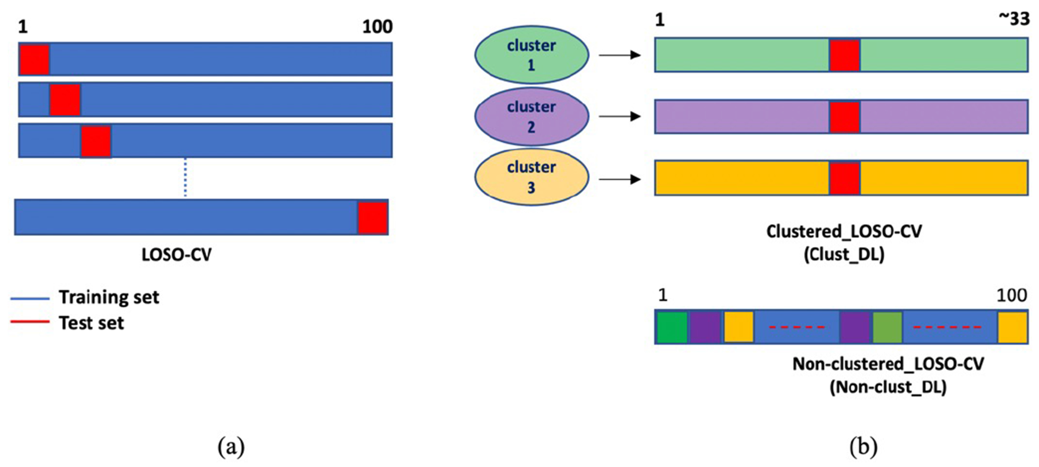
(a): General process in LOSO cross-validation. At each step, one data is used as test data and others for training. (b): Difference between clustered training (clust-DL) using the three clusters and standard training (nonclust-DL). Data in each cluster used as a training set in clust-DL. Test results of standard training using all the data were computed and corresponding data from each cluster were picked from the test results.

Table III shows the quantitative results of SPECT_DL and SPECT_NC, compared with the reference for both clustered and non-clustered training by using ResUNet LOSO CV. The DL approach improved the similarity of SPECT_DL to the reference SPECT_CTAC for NRMSE, PSNR, and SSIM metrics, compared to that of SPECT_NC to the reference, for all cases.

TABLE III.

Quantitative comparison of clustered training versus standard training using all the data (mean ± SD).

clust/non-clust training	NRMSE	PSNR	SSIM
G1NC	0.218±0.0878	32.3926±2.8526	0.9894±0.0063
G1clust-DL	0.1359±0.0698	36.8832±3.8087	0.9954±0.0040
G1nonclut-DL	0.1266±0.0665	37.4576±3.5191	0.9961±0.0033
G2NC	0.2342±0.0701	31.0235±2.7094	0.9854±0.0089
G2clust-DL	0.1677±0.0809	34.4445±3.8312	0.9926±0.0061
G2nonclust-DL	0.1464±0.0605	35.4327±3.5710	0.9938±0.0051
G3NC	0.2267±0.0738	31.7770±3.3316	0.9881±0.0070
G3clust-DL	0.1788±0.1918	35.1891±3.9203	0.9928±0.0119
G3nonclust-DL	0.1464±0.0706	35.8799±3.1448	0.9952±0.0035
Totalclust	0.1595±0.1250	35.5851±3.9526	0.9937±0.0079
Totalnonclust	0.1391±0.0661	36.3250±3.5012	0.9951±0.0041

Approximately 70% more data allowed 12.8% improvement in the overall NRMSE result (improvements for G1, G2, and G3 are 6.84%, 12.7%, and 18.12% respectively, Fig. 14). Data with more uniform polar patterns (G1) benefit less by adding more data (Fig. 14). The p-values for the clustered and standard training are 0.182, 0.003, and 0.179 for group 1, 2, and 3 respectively. Adding data is more beneficial for groups which contains data with nonuniform patterns (G2 and G3). This observation can help us in prioritizing the type of data we collect later.

Fig. 14.

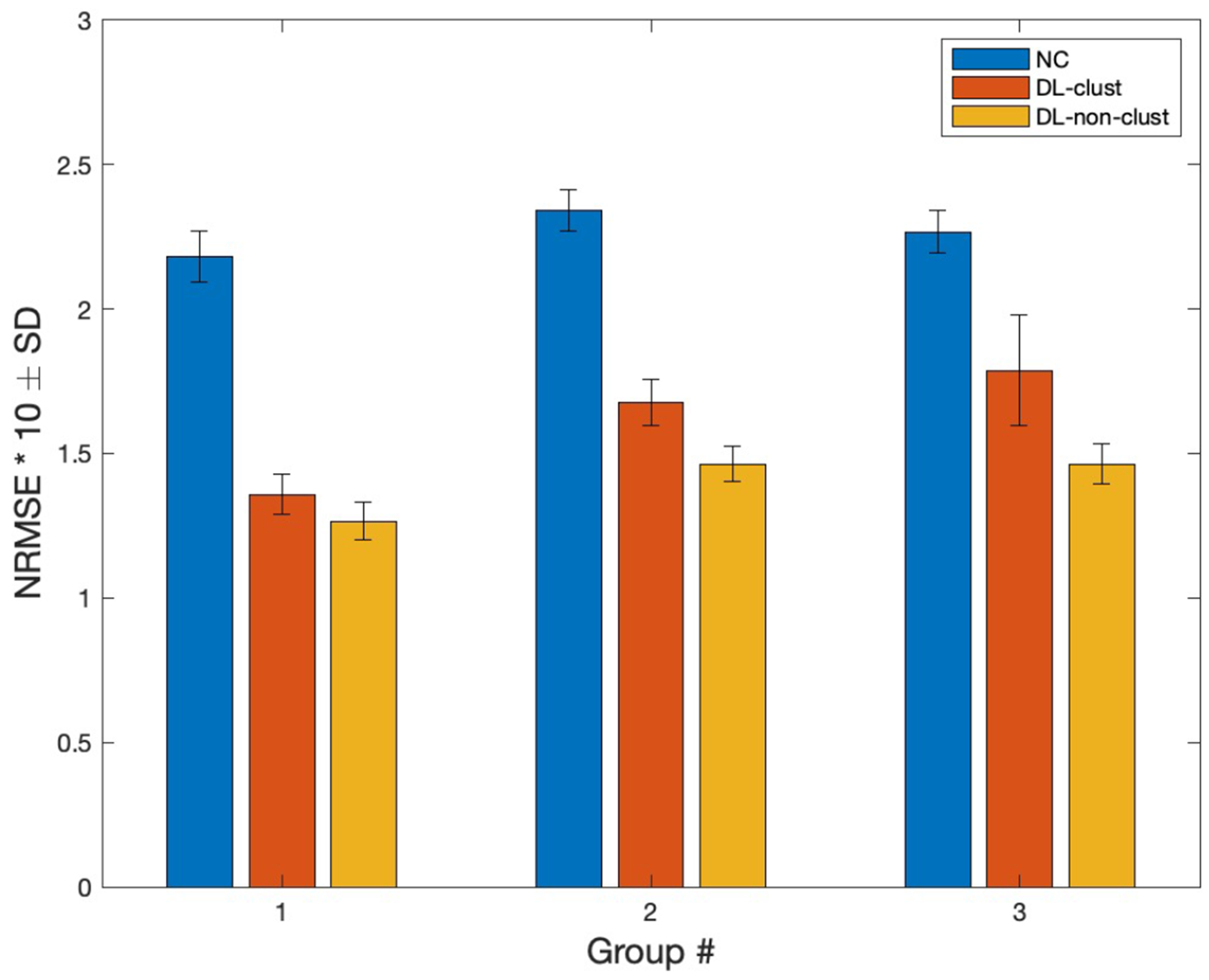
NRMSE comparison of DL results from clustered and non-clustered (standard) training for three groups generated by the BIRCH algorithm in the t-SNE space. Error bars represents the standard deviation (SD).

We used ResUNet for generating all the results of this subsection III-B.

IV. Discussion

Despite increasing DL-based studies for the AC task, they rarely translate into clinical practice due to performance inconsistency. Thus, it is important to validate the robustness of DL models to new incoming data towards clinical translation. Previously, we investigated the feasibility of using a DL approach for SPECT AC in the image domain and demonstrated the potential clinical values of the proposed method in the stand-alone SPECT systems that occupy 80% of the current market share [8], [9]. Incorporating the DL-based AC into clinical practice can improve the diagnostic accuracy of MPIs by eliminating the attenuation artifacts [3], [40] and also reduce the radiation dose from CT, which can benefit pediatric patients who are more at risk of radiation [41]. However, performance variability across patients is one of the obstacles that hinder the clinical translation of our direct DL-based AC for SPECT MPI. This variability comes from the fact that a network learns attenuation patterns statistically from data whose distribution may be different from the new data, which is distinct from physics-based conventional methods that use attenuation maps generated from CT images.

As an initial investigation to address a potential performance variability, we demonstrated how an advanced network architecture can improve the global quantitative results. We also demonstrate training with clustered datasets has the potential to reduce the variability concerning attenuation artifacts in SPECTNC across patients with uniform attenuation pattern of polar maps.

This study demonstrated potential benefits. First, it raises awareness toward performance variability as one of the important factors for the clinical translation of DL-based AC approaches. For the clinical translation of DL-based approaches, they must be held accountable to the same rigorous standards that traditional methods follow. Accuracy and performance consistency are two important pillars of developing reliable DL-based methods for SPECT AC. Second, it shows that the performance of the model does not have a linear relationship with the number of training data (III-B4). In the results, adding training data from more nonuniform polar patterns is more beneficial to the learning process than adding data with uniform patterns. Intuitively from a computer vision perspective, it is easier for networks to learn important features from uniform patterns and is the reason that the network benefits more in learning from the data with unique nonuniform patterns. Third, results from section III-B2 imply that the training set which consists of data with a more similar distribution compared to the training set with random data, can help the learning process and generate results with less variability. Fourth, as a preprocessing step for the network to learn better, one can remove low count voxels outside the myocardium (background noise) by binary masking [30]. However, the right ventricle cannot be seen in SPECT_DL anymore and for diagnostic purposes, physicians prefer to look at the whole image including the background. The WCycleGAN enables skipping the background removal step while improving the NRMSE by 8.9%. Fifth, use of an advanced network does not improve the regional results when we have limited data for the training and results are more subject specific (Fig. 2 and Fig. 3). In the future we will investigate advantages of model-centric DL methods (advanced architectures) with a larger and more diverse dataset for regional improvement of SPECT AC. However, in this study with limited data, an advanced network can only improve the global results which are computed based on the averaged pixel-to-pixel comparison of the SPECT_DL and SPECT_CTAC.

Despite the potential benefits, this study has several limitations. First, the limited data (only 100 patches) might not include diverse attenuation patterns in the database. The results show that data with nonuniform patterns did not benefit from the clustered training as much as data with more uniform distribution (group 1) did. In addition, segmental results of attenuation correction using WCycleGAN may improve compare to the U-Net if the networks are trained with larger dataset. Second, meta information including the patient’s height, weight, and clinical interpretation of images was missing due to the deidentification, and the effect of these on the current results could not be analyzed. Finally, cycle consistency used in the objective function enforces one-to-one mapping at pixel level and there is no information loss during the translation which can generate irrelevant texture artifacts. However, non-corrected and attenuation corrected images which were used here do not have drastically different textures or complex patterns. Therefore, it is likely that the cycle consistency has less effect on generating texture-related artifacts in our application.

In future work, we plan to expand our current dataset to include more diverse cases and studying how the training and evaluation would be different with a large normative dataset. Furthermore, with a larger dataset we will investigate unsupervised DL techniques to cluster the images into sub-grouped training sets [42], [25].

V. Conclusion

In this study, we investigated methods to overcome the performance variability of DL-based models with limited data for the SPECT AC task. The results demonstrated that the WCycleGAN as an advanced network can improve the accuracy of global measurements and has the potential to reduce the performance variability across the patients. In addition, the results demonstrated that clustering of the data in the low-dimensional t-SNE space can enable deep learning models to learn attenuation patterns more effectively.

Appendix

OPTIMAL NUMBER OF PRINCIPAL COMPONENTS FOR THE t-SNE TECHNIQUE

One of the hyperparameters in the t-SNE which can reduce the computational cost is the number of input principal components. Principal components are eigenvectors calculated from the eigen decomposition of the data covariance matrix. As a result of this decomposition, the k largest eigenvalues and corresponding eigenvectors (principal components (PC)) can be computed. The PCs can be used as a new orthogonal basis to project the data to a lower-dimensional space. The first few principal components often sufficiently explain the data variance. We chose the first 4 principal components as the input to the t-SNE algorithm.

To choose how many PCs are sufficient to span the new space, we kept the PCs containing correlations larger than the random sampling error within our dataset [43]. For evaluating the error, we shuffle the values of each segment and between different polar plots independently to remove coloration between segment values. We have 100 SPECT_NC data and each has 17 segments polar plot which can be represented as a 100 × 17 matrix. Each row of the new shuffled matrix has a random value taken from other polar plots at the same segment. Fig. 15 shows the eigen spectrum for the original and the shuffled data. As can be seen, the first 4 PCs are enough to explain the variance of the original data to an extent which is distinguishable from the sampling error. These top 4 PCs can cumulatively explain more than 83% of the variance within the data.

Fig. 15.

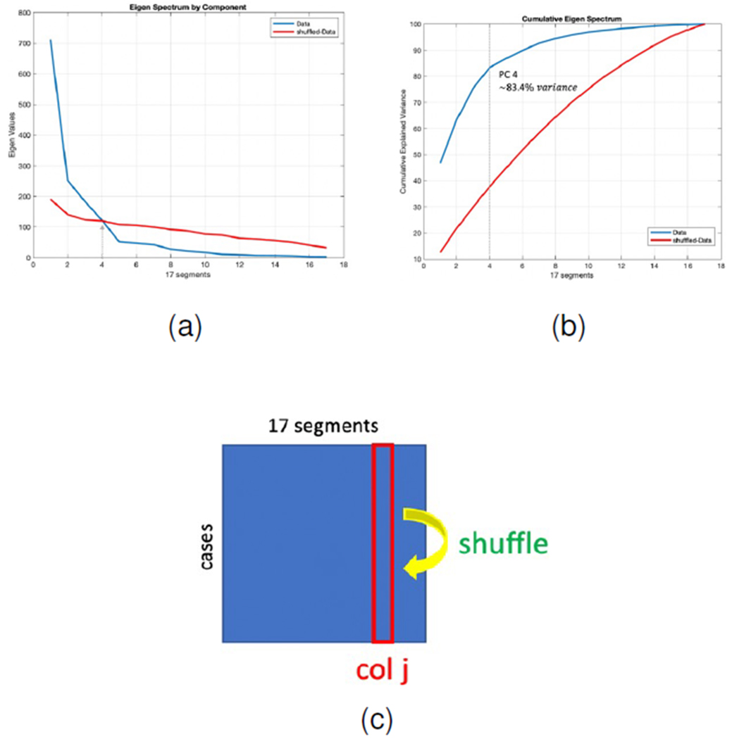
(a): Eigen spectrum comparison of the original and shuffled polar plots. (b): Cumulative explained variance of the original and shuffled data, first 4 PCs explain more than 83% of the data variance. (c): Schematic picture showing how data is shuffled to remove correlation between the segments

References

- [1].Abbott BG, Case JA, Dorbala S, Einstein AJ, Galt JR, Pagnanelli R, Bullock-Palmer RP, Soman P, and Wells RG. “Contemporary cardiac SPECT imaging—innovations and best practices: an information statement from the American Society of Nuclear Cardiology,” in Circulation: Cardiovascular Imaging, vol. 11, no. 9, pp. e000020, 2018. [DOI] [PubMed] [Google Scholar]
- [2].DePuey EG. “How to detect and avoid myocardial perfusion SPECT artifacts.” J.N.M, vol, no. 4, pp. 699–702, 1994. [PubMed] [Google Scholar]
- [3].Patchett ND. “Does Improved Technology in SPECT Myocardial Perfusion Imaging Reduce Downstream Costs? An Observational Study,” International Journal of Radiology and Imaging Technology, vol. 3, no. 1, 2017. [Google Scholar]
- [4].Ficaro EP, Fessler JA, Shreve PD, Kritzman JN, Rose PA, and Corbett JR. “Simultaneous Transmission/Emission Myocardial Perfusion Tomography,” Circulation, vol. 93, no. 3, pp. 463–473, 1996. [DOI] [PubMed] [Google Scholar]
- [5].Gallowitsch HJ, Sykora J, Mikosch P, Kresnik E, Unterweger O, Molnar M, Grimm G, and Lind P. “Attenuation-corrected thallium-201 single-photon emission tomography using a gadolinium-153 moving line source: clinical value and the impact of attenuation correction on the extent and severity of perfusion abnormalities,” European Journal of Nuclear Medicine and Molecular Imaging, vol. 25, no. 3, pp. 220–228, 1998. [DOI] [PubMed] [Google Scholar]
- [6].Singh B, Bateman T, Case J, and Heller G. “Attenuation artifact, attenuation correction, and the future of myocardial perfusion SPECT,” Journal of Nuclear Cardiology, vol. 14, no. 2, pp. 153–164, 2007. [DOI] [PubMed] [Google Scholar]
- [7].Heller G. “American Society of Nuclear Cardiology and Society of Nuclear Medicine joint position statement: attenuation correction of myocardial perfusion SPECT scintigraphy,” Journal of Nuclear Cardiology, vol. 11, no. 2, p. 229, 2004. [DOI] [PubMed] [Google Scholar]
- [8].“Global SPECT Market 2017-2021”, [Online]. Available: https://www.technavio.com/report/global-medical-imaging-global-spect-market-2017-2021.
- [9].Torkaman M, Yang J, Shi L, Wang R, Miller EJ, Sinusas AJ, Liu C, Gullberg GT, and Seo Y. “Direct image-based attenuation correction using conditional generative adversarial network for SPECT myocardial perfusion imaging,” Medical Imaging 2021: Biomedical Applications in Molecular, Structural, and Functional Imaging, 2021. [DOI] [PMC free article] [PubMed] [Google Scholar]
- [10].He K, Zhang X, Ren S, and Sun J. “Delving Deep into Rectifiers: Surpassing Human-Level Performance on ImageNet Classification,” 2015 IEEE International Conference on Computer Vision (ICCV), 2015. [Google Scholar]
- [11].Taigman Y, Yang M, Ranzato M, and Wolf L. “DeepFace: Closing the Gap to Human-Level Performance in Face Verification,” 2014 IEEE Conference on Computer Vision and Pattern Recognition, 2014. [Google Scholar]
- [12].Sendak MP , D’Arcy J, Kashyap S, Gao M, Nichols M, Corey K, Ratliff W, and Balu S. “A path for translation of machine learning products into healthcare delivery,” EMJ Innov, vol 10, pp. 19–00172, 2020. [Google Scholar]
- [13].Antun V, Renna F, Poon C, Adcock B, and Hansen AC. “On instabilities of deep learning in image reconstruction and the potential costs of AI,” Proc. National Academy of Sciences, vol 117, no. 48, pp. 30088–30095, 2020. [DOI] [PMC free article] [PubMed] [Google Scholar]
- [14].Torres-Velázquez M, Chen WJ, Li X, and McMillan AB. “Application and construction of deep learning networks in medical imaging”, IEEE transactions on radiation and plasma medical sciences, 2020. [DOI] [PMC free article] [PubMed] [Google Scholar]
- [15].Fawzi A, Moosavi-Dezfooli S-M, and Frossard P. “The Robustness of Deep Networks: A Geometrical Perspective,” IEEE Signal Processing Magazine, vol. 34, no. 6, pp. 50–62, 2017. [Google Scholar]
- [16].Kanbak C, Moosavi-Dezfooli S-M, and Frossard P. “Geometric Robustness of Deep Networks: Analysis and Improvement,” 2018 IEEE/CVF Conference on Computer Vision and Pattern Recognition, 2018. [Google Scholar]
- [17].Moosavi-Dezfooli S-M, Fawzi A, and Frossard P. “DeepFool: A Simple and Accurate Method to Fool Deep Neural Networks,” Proc. CVPR, pp. 2574–2582, 2016. [Google Scholar]
- [18].Szegedy C, Zaremba W, Sutskever I, Bruna J, Erhan D, Goodfellow I, and, Fergus R. “Intriguing properties of neural networks,” arXiv preprint arXiv:1312.6199, 2013. [Google Scholar]
- [19].Shaikhina T and Khovanova NA. “Handling limited datasets with neural networks in medical applications: A small-data approach,” Artificial Intelligence in Medicine, vol. 75, pp. 51–63, 2017. [DOI] [PubMed] [Google Scholar]
- [20].Cunningham P, Carney J, and Jacob S. “Stability problems with artificial neural networks and the ensemble solution,” Artificial Intelligence in Medicine, vol. 20, no. 3, pp. 217–225, 2000. [DOI] [PubMed] [Google Scholar]
- [21].Lee JS. “A Review of Deep-Learning-Based Approaches for Attenuation Correction in Positron Emission Tomography”, IEEE Transactions on Radiation and Plasma Medical Sciences, vol 5, no. 2, pp.160–184, 2020. [Google Scholar]
- [22].Arabi H, Zeng G, Zheng G, and Zaidi H. “Novel adversarial semantic structure deep learning for MRI-guided attenuation correction in brain PET/MRI,” Eur. J. Nucl. Med. Mol. Imag, vol. 46, no. 13, pp. 2746–2759, 2019. [DOI] [PubMed] [Google Scholar]
- [23].Bradshaw TJ, Zhao G, Jang H, Liu F, and McMillan AB. “Feasibility of deep learning-based PET/MR attenuation correction in the pelvis using only diagnostic MR images,” Tomography, vol. 4, no. 3, pp. 138–147, 2018. [DOI] [PMC free article] [PubMed] [Google Scholar]
- [24].Liu F, Jang H, Kijowski R, Bradshaw T, and McMillan AB. “Deep learning MR imaging-based attenuation correction for PET/MR imaging,” Radiology, vol. 286, no. 2, pp. 676–684, 2018. [DOI] [PMC free article] [PubMed] [Google Scholar]
- [25].Yang J, Parikh D, and Batra D. “Joint Unsupervised Learning of Deep Representations and Image Clusters,” 2016 IEEE Conference on Computer Vision and Pattern Recognition (CVPR), 2016. [Google Scholar]
- [26].Shi L, Onofrey JA, Revilla EM, Toyonaga T, Menard D, Ankrah J, Carson RE, Liu C, and Lu Y. “A novel loss function incorporating imaging acquisition physics for PET attenuation map generation using deep learning,” In International Conference on Medical Image Computing and Computer-Assisted Intervention, pp. 723–731, 2019 [Google Scholar]
- [27].Hwang D, Kim KY, Kang SK, Seo S, Paeng JC, Lee DS, S. D, and Lee JS. “Improving the accuracy of simultaneously reconstructed activity and attenuation maps using deep learning,” J. Nucl. Med, vol. 59, no. 10, pp. 1624–1629, 2018. [DOI] [PubMed] [Google Scholar]
- [28].Liu F, Jang H, Kijowski R, Zhao G, Bradshaw T, and McMillan AB. “A deep learning approach for 18F-FDG PET attenuation correction,” EJNMMI Phys, vol. 5, p. 24, Dec. 2018. [DOI] [PMC free article] [PubMed] [Google Scholar]
- [29].Dong X, Lei Y, Wang T, Higgins K, Liu T, Curran WJ, Mao H, Nye JA, and Yang X. “Deep learning-based attenuation correction in the absence of structural information for whole-body positron emission tomography imaging,” Physics in Medicine & Biology, vol. 65, no. 5, p.055011, 2020. [DOI] [PMC free article] [PubMed] [Google Scholar]
- [30].Yang J, Shi L, Wang R, Miller EJ, Sinusas AJ, Liu CJ, Gullberg GT, and Seo Y. “Direct Attenuation Correction Using Deep Learning for Cardiac SPECT: A Feasibility Study,” Journal of Nuclear Medicine, 2021. [DOI] [PMC free article] [PubMed] [Google Scholar]
- [31].Zhu J-Y, Park T, Isola P, and Efros AA. “Unpaired Image-to-Image Translation Using Cycle-Consistent Adversarial Networks,” 2017 IEEE International Conference on Computer Vision (ICCV), 2017. [Google Scholar]
- [32].Ronneberger O. “Invited Talk: U-Net Convolutional Networks for Biomedical Image Segmentation,” Informatik aktuell Bildverarbeitung für die Medizin, pp. 3–3, 2017. [Google Scholar]
- [33].He K, Zhang X, Ren S, and Sun J. “Deep Residual Learning for Image Recognition,” 2016 IEEE Conference on Computer Vision and Pattern Recognition (CVPR), 2016. [Google Scholar]
- [34].Isola P, Zhu J-Y, Zhou T, and Efros AA. “Image-to-Image Translation with Conditional Adversarial Networks,” 2017 IEEE Conference on Computer Vision and Pattern Recognition (CVPR), 2017. [Google Scholar]
- [35].Goodfellow IJ, Pouget-Abadie J, Mirza M, Xu B, Warde-Farley D, Ozair S, Courville A, and Bengio Y. “Generative adversarial networks,” arXiv preprint arXiv:1406.2661, 2014. [Google Scholar]
- [36].Arjovsky M, Chintala S, and Bottou L. “Wasserstein generative adversarial networks,” International conference on machine learning PMLR, pp. 214–223, 2017. [Google Scholar]
- [37].Hinton G, Srivastava N, and Swersky K, “Neural networks for machine learning lecture 6a overview of mini-batch gradient descent,” Cited on, vol. 14, no. 8, 2012. [Google Scholar]
- [38].Van der Maaten L, and Hinton G. “Visualizing data using t-SNE,” Journal of machine learning research, vol. 9, no. 11. 2008 [Google Scholar]
- [39].Zhang T, Ramakrishnan R, and Livny M, “Birch,” Proceedings of the 1996 ACM SIGMOD international conference on Management of data - SIGMOD, 1996. [Google Scholar]
- [40].Rahmim A and Zaidi H. “PET versus SPECT: strengths, limitations and challenges,” Nuclear Medicine Communications, vol. 29, no. 3, pp. 193–207, 2008. [DOI] [PubMed] [Google Scholar]
- [41].Núñez M, Prakash V, Vila R, Mut F, Alonso O, and Hutton BF. “Attenuation correction for lung SPECT: evidence of need and validation of an attenuation map derived from the emission data,” European Journal of Nuclear Medicine and Molecular Imaging, vol. 36, no. 7, pp. 1076–1089, 2009. [DOI] [PubMed] [Google Scholar]
- [42].Chang J, Wang L, Meng G, Xiang S, and Pan C. “Deep Adaptive Image Clustering,” 2017 IEEE International Conference on Computer Vision (ICCV), 2017. [Google Scholar]
- [43].Berman GJ, Choi DM, Bialek W, and Shaevitz JW. “Mapping the stereotyped behavior of freely moving fruit flies,” Journal of The Royal Society Interface, vol. 11, no. 99, p. 20140672, 2014. [DOI] [PMC free article] [PubMed] [Google Scholar]