Inferring Phenotypic Trait Evolution on Large Trees With Many Incomplete Measurements

Abstract

Comparative biologists are often interested in inferring covariation between multiple biological traits sampled across numerous related taxa. To properly study these relationships, we must control for the shared evolutionary history of the taxa to avoid spurious inference. An additional challenge arises as obtaining a full suite of measurements becomes increasingly difficult with increasing taxa. This generally necessitates data imputation or integration, and existing control techniques typically scale poorly as the number of taxa increases. We propose an inference technique that integrates out missing measurements analytically and scales linearly with the number of taxa by using a post-order traversal algorithm under a multivariate Brownian diffusion (MBD) model to characterize trait evolution. We further exploit this technique to extend the MBD model to account for sampling error or non-heritable residual variance. We test these methods to examine mammalian life history traits, prokaryotic genomic and phenotypic traits, and HIV infection traits. We find computational efficiency increases that top two orders-of-magnitude over current best practices. While we focus on the utility of this algorithm in phylogenetic comparative methods, our approach generalizes to solve long-standing challenges in computing the likelihood for matrix-normal and multivariate normal distributions with missing data at scale.

1. INTRODUCTION

Phylogenetic comparative methods explore the relationships between different biological phenotypes across sets of organisms. To properly understand these phenotypic trait relationships, methods must adjust for the shared evolutionary history of the taxa (?). Molecular sequences from emerging sequencing technology and high-throughput biological experimentation enable such phylogenetic adjustment for rapidly growing numbers of taxa and increasing numbers of trait measurements. Comparative studies incorporating dense taxonomic sampling create the potential for new research into general patterns in phenotypic evolution, key differences between subgroups and the relationship between phenotypic and genetic evolutionary dynamics. Unfortunately, many phylogenetic comparative methods remain poorly equipped to handle these research questions at scale.

Popular methods often assume an underlying Brownian diffusion process acts along each branch of a phylogenetic tree, such that the traits are multivariate normally distributed. Revell (2012) and Adams (2014), for example, parameterize this distribution in terms of a highly-structured variance-covariance matrix that characterizes the tree and trait covariation. Computational work to invert this matrix to evaluate the multivariate normal likelihood scales cubically with the number of taxa. This work stands even more troublesome when the phylogenetic tree remains unknown and requires joint inference with the trait process, necessitating repeated inversion. Freckleton (2012), Pybus et al. (2012), and Ho and Ané (2014) all independently develop algorithms that take advantage of the matrix-normal structure of the data under the MBD model to evaluate the likelihood. Using the tree structure, these algorithms then scale linearly with the number of taxa with complete data, but this ideal run-time currently stumbles when trait measurements are missing.

As the number of taxa grows large, measuring a complete suite of traits for all taxa becomes increasingly challenging. While stripping any rows of data with missing values may create a “complete” data set, this procedure both reduces statistical power and can introduce bias (Nakagawa and Freckleton 2008). Recent solutions to this problem that take advantage of all available data include those by Goolsby (2017), Tolkoff et al. (2017), Bastide et al. (2018), and Mitov et al. (2020). Tolkoff et al. (2017), for example, treat the missing data points as unknown model parameters and integrate them out via Markov Chain Monte Carlo (MCMC). This method, however, requires iterative manipulation of the likelihood function on a per-taxon basis and remains computationally prohibitive for large trees. Alternatively, Goolsby (2017), Bastide et al. (2018), and Mitov et al. (2020) take a different approach and develop algorithms that can compute the likelihood of the observed data only in linear time with respect to the number of taxa. However, the inference strategy of all three groups (implemented in Rphylopars (Goolsby et al. 2017), PCMFit (Mitov et al. 2019), and PhylogeneticEM (Bastide et al. 2018) respectively) rely on maximum likelihood estimation (MLE) regimes that assume the phylogenetic tree is known a priori. While this assumption may be appropriate when the phylogenetic tree is known with a high degree of certainty, this is not the case for many practical problems. If there is any uncertainty in the tree, these methods will likely be both biased and over-confident in their estimates.

In this paper, we reformulate evaluation of the data likelihood function under a Brownian diffusion process on a tree such that we achieve the marginalized likelihood of the observed trait measurements only. This innovation arises from thinking about observed tip traits as multivariate normally distributed with infinite precision in their sampling, while missing traits have zero precision, and appropriately propagating these precisions up the tree through dynamic programming involving an unusual matrix pseudo-inverse definition. This pseudo-inverse finds similar use, but independent discovery, in Bastide et al. (2018). Unlike previous approaches, the integration avoids EM iteration making simultaneous inference with the phylogeny practical and enables researchers to analyze all available measurements when inferring the trait relationships. Surprisingly, we can still evaluate the observed-data likelihood in linear time with respect to the number of taxa. The price to be paid is that computation now scales cubically, rather than quadratically, in the number of traits. This remains a small price since the number of taxa is often orders-of-magnitude larger than the number of traits. It is also notable that this method has applications beyond phylogenetic comparative methods and can be used more generally in a special class of matrix-normal and multivariate normal distributions with missing data. This has been a long standing problem in statistics since at least the 1930’s (Wilks 1932), with more recent work by Dominici et al. (2000); Cantet et al. (2004); Allen and Tibshirani (2010); and Glanz and Carvalho (2018). One important limitation to our approach is that it assumes data are missing at random (Little and Rubin 1987) which is inappropriate for many data sets.

We also demonstrate how this framework can be easily extended to incorporate residual variance in the MBD model, which is only one of many possible model extensions. Our strategy of analytically marginalizing the observed data likelihood extends seamlessly to this and other model extensions and allows for efficient inference on these models while maintaining likelihood computations that scale linearly with the number of taxa. These extensions open up lines of inquiry not available in the simple MBD model. In particular, including residual variance in the model enables inference of phylogenetic heritability.

We demonstrate the broad utility of our algorithm to compute the marginalized likelihood through three examples. First, we examine covariation in mammalian life history traits using data on 3649 taxa from the PanTHERIA ecological database (Jones et al. 2009). Second, we use our new efficient algorithm to simultaneously evaluate several theories regarding prokaryotic evolutionary theory. We use data from NCBI Genome and a recent study by Goberna and Verdú (2016), along with matching 16S sequences from the ARB Silva Database (Ludwig et al. 2004), to jointly infer both the phylogenetic tree and evolutionary correlation between several prokaryotic genotypic and phenotypic traits. Finally, we apply our multivariate residual variance model extension to data presented by Blanquart et al. (2017) concerning HIV virulence to evaluate the heritability of HIV viral load and CD4 T-cell decline. We compare the computation speed of our analytical integration method against current best-practice methods and observed increases in speed that top two orders-of-magnitude.

2. PHENOTYPIC DIFFUSION ON TREES

Consider a data-complete collection Y = (Y₁, …, Y_N)^t where Y_i = (Y_i1, …, Y_iP)^t of P real-valued phenotypic traits measured across N biological taxa. Relating the taxa stands a known and fixed or unknown and random phylogeny $\mathcal{F}$ that is a bifurcating, directed acyclic graph whose 2N − 1 vertices originate with a degree-2 root node ν_2N−1 and terminate with degree-1 tip nodes (ν₁, …, ν_N) that correspond to the N taxa. Linking vertices are edge weights or branch lengths (t₁, …, t_2N−2). Let X_k = (X_k1, …, X_kP) be latent values of the traits at node ν_k on the tree for k = 1, …, 2N − 1. For tip nodes i = 1, …, N, we posit a stochastic link p(Y_i |X_i) where Y_i is drawn from some distribution parameterized by X_i and other hyperparameters (see Figure 1). Comparative methods standardly assume that the density p(Y_i |X_i) is degenerate at X_i (i.e. Y_i = X_i with probability 1), but we relax this assumption in future sections.

Figure 1:

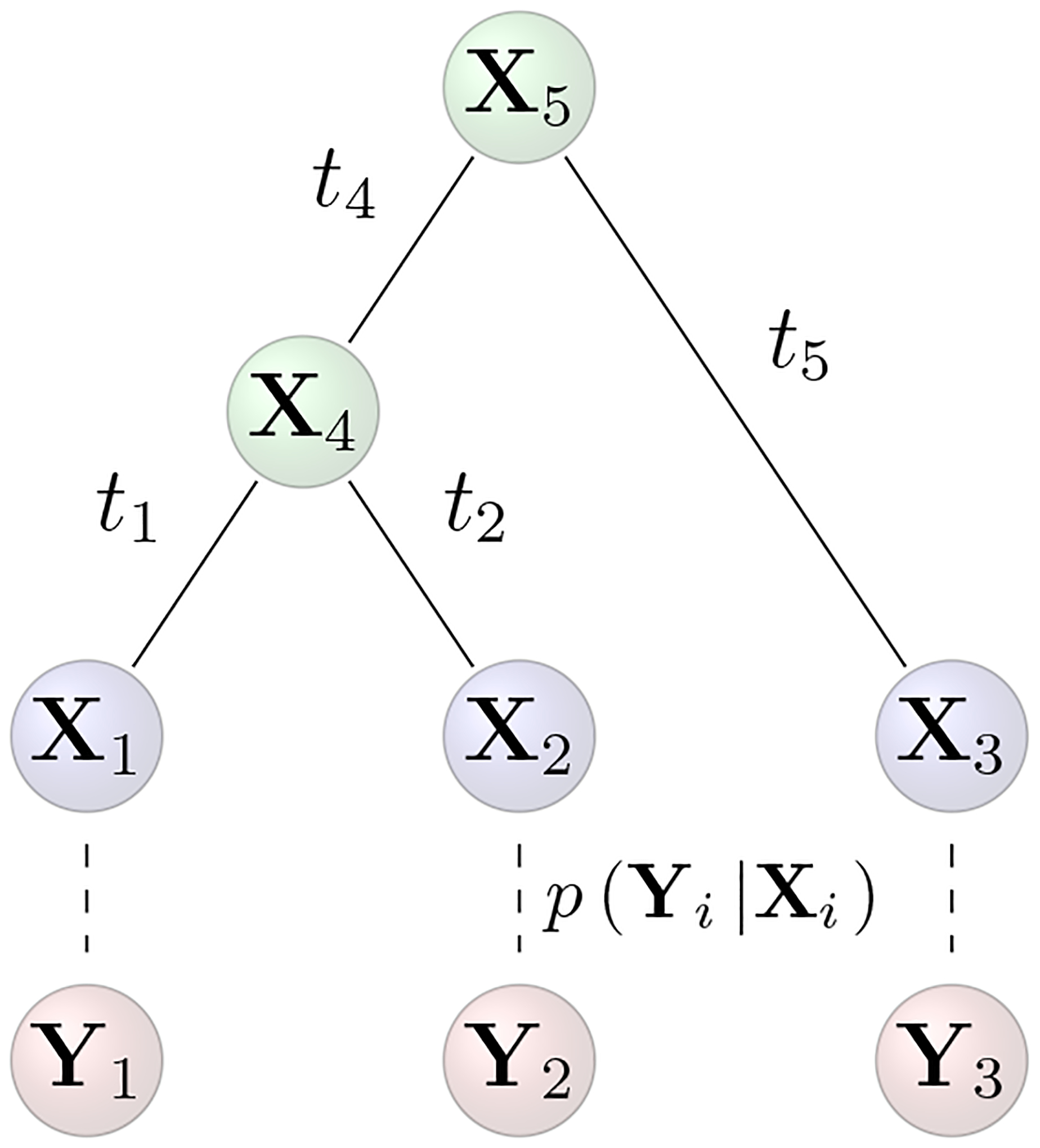
Schematic of diffusion model with stochastic link function. The data Y = (Y₁, Y₂, Y₃)^t arise from latent values X_i at the tips of the tree via the stochastic link function p(Y_i |X_i) for i = 1, …, N.

The most common phenotypic model of evolution (?) assumes a multivariate Brownian diffusion process acts conditionally independently along each branch generating a multivariate normal (MVN) increment,

$$X_k~\text{MVN}\left(X_{\text{pa}(k)},t_k\Sigma \right)\text{ for }k=1,\dots ,2N-2,$$ (1)

centered around the realized value X_pa(k) at its parent node and variance proportional to an estimable P × P positive-definite matrix Σ. Since the trait values at the root are also unknown, Pybus et al. (2012) suggest further assuming $X_{2N-1}~\text{MVN}\left({\mu }_0,{\kappa }_0^{-1}\Sigma \right)$ with fixed prior mean μ₀ and sample-size κ₀.

2.1. Computation of Observed Data Likelihood

When there are no missing data and under our standard assumption that p(Y_i |X_i) is degenerate, integrating out unobserved internal and root node traits leads to a seemingly simple expression for the data likelihood $p\left(Y\mid \Sigma ,\mathcal{F},{\mu }_0,{\kappa }_0\right)$ (Freckleton 2012; Vrancken et al. 2015). Namely, Y is matrix-normal (MN) distributed around mean $1_N{\mu }_0^t$, with across-row variance $\mathbf{\Upsilon }+{\kappa }_0^{-1}{J}_N$ and across-column variance Σ, where 1_N is a vector of length N populated by ones, $J_N=1_N{1}_N^t$, and ϒ is a deterministic function of $\mathcal{F}$. Specifically, element ϒ_ii′ measures shared evolutionary history and equals the sum of the branch lengths from the root to the most recent common ancestral node of taxa i and i′ when i ≠ i′ or the sum of the branch lengths from the root to taxon i otherwise. For example, in Figure 1, ϒ₁₂ = t₄ and ϒ₁₁ = t₁ + t₄. One can evaluate this highly structured matrix-normal likelihood function with computational complexity $\mathcal{O}\left(N{P}^2\right)$ given the acyclic nature of $\mathcal{F}$. When some data points are missing, however, the observed-data likelihood is no longer matrix-normal and new approaches are needed. This becomes increasingly urgent as the prevalence of missing observations grows with the size of trait data sets. In this context we wish to compute

$$p\left(Y^{\text{obs }}\mid \Sigma ,\mathcal{F},{\mu }_0,{\kappa }_0\right)=\int p\left(Y^{\text{obs }},Y^{\text{mis }}\mid \Sigma ,\mathcal{F},{\mu }_0,{\kappa }_0\right)\text{d}{Y}^{\text{mis }},$$ (2)

where Y^obs and Y^mis contain the observed and missing trait values, respectively.

The two simplest strategies for calculating the observed-data likelihood are, unfortunately, computationally prohibitive for most large problems. One such solution forfeits the MN structure of the data in favor a simple expression of the observed-data likelihood. This strategy uses the fact that the matrix-normal distribution of Y can also be expressed as

$$\text{vec}\left[Y\mid \Sigma ,\mathcal{F},{\mu }_0,{\kappa }_0\right]~\text{MVN}\left(\text{vec}\left[1_N{\mu }_0^t\right],\Sigma \otimes \left(\mathbf{\Upsilon }+{\kappa }_0^{-1}{J}_N\right)\right),$$ (3)

using the Kronecker product ⊗. Assuming data are missing at random (Little and Rubin 1987), one can simply remove the rows and columns of $\text{vec}\left[1_N{\mu }_0^t\right]$ and $\Sigma \otimes \left(\mathbf{\Upsilon }+{\kappa }_0^{-1}{J}_N\right)$ corresponding to the missing data and compute the likelihood for this NP − M′ dimensional MVN distribution, where M′ is the number of missing measurements. This likelihood calculation carries the onerous computational complexity $\mathcal{O}\left({\left(NP-M^{\prime }\right)}^3\right)$. Alternatively, from a Bayesian perspective, one could numerically integrate out the missing data by treating each missing data point as an unknown model parameter and employing MCMC to sample each value. This strategy restores the matrix-normal structure, but requires the likelihood be evaluated each time one samples a missing data point. This results in computation complexity of at least $\mathcal{O}\left(N{P}^{2}M\right)$, where M is the number of taxa with missing measurements. Because M often scales with N, this method remains prohibitively slow for many data sets with large N. Our goal is to integrate out these missing values analytically using a dynamic programming algorithm in order to bring run time down to a much more manageable $\mathcal{O}\left(N{P}^3\right)$.

2.1.1. Missing Data Definitions and Operations

To develop our algorithm, we first introduce some useful abstractions and notation. At each tip in $\mathcal{F}$, information about each of the P traits comes in one of three forms: a trait value may be directly observed, latent, or completely missing. When directly observed, we posit without loss of generality that the value arises from a normal distribution centered at the observed value with infinite precision. We assume that trait data that arise from latent values are jointly multivariate normally distributed about the unknown latent values with known or estimable precision. Finally, a completely missing value arises also without loss of generality from a normal distribution centered at 0 with zero precision. To formalize this, for tip i = 1, …, N, we construct a permutation matrix C_i that groups traits in directly observed, latent, and completely missing order and populate a pseudo-precision matrix

$$P_i=C_i\text{\hspace{0.17em}diag\hspace{0.17em}}\left[\infty I,R_i,0I\right]C_i^t,$$ (4)

where diag[·] is a function that arranges its constituent elements into block-diagonal form and R_i is the latent block precision. Note that any block may be 0-dimensional. This construction arbitrarily forces off-diagonal elements of P_i involving directly observed and completely missing traits to equal 0 and plays an important role in simplifying computations.

We additionally define a series of operations that we will find useful for defining this algorithm. We define the pseudo-inverse

$$P_i^{-}=C_i\text{\hspace{0.17em}diag\hspace{0.17em}}\left[0I,R_i^{-1},\infty I\right]C_i^t.$$ (5)

We define the pseudo-determinant dêt() as the product of the non-zero singular values. We also define the matrix δ_i = diag[δ_i1, …, δ_iP] for i = 1, …, N, where δ_ij is an indicator variable which takes a value of 1 if trait Y_ij is observed or latent and 0 if it is missing. Lastly, we define the possibly degenerate multivariate normal density function

$$\text{log\hspace{0.17em}}\widehat{\varphi }(z;\mu ,P)=\frac{1}{2}\text{log\hspace{0.17em}}\widehat{\text{det\hspace{0.17em}}}(P)-\frac{\text{rank}(P)}{2}\text{log\hspace{0.17em}}2\pi -\frac{1}{2}{(z-\mu )}^{t}P(z-\mu ),$$

for some argument z, mean μ and precision P of appropriate dimensions.

2.1.2. Post-Order Observed Data Likelihood Algorithm

Our goal is to efficiently compute the likelihood $p\left(Y^{\text{obs}}\mid \Sigma ,\mathcal{F},{\mu }_0,{\kappa }_0\right)$. Following from Pybus et al. (2012), we perform a post-order traversal where we calculate the observed-data partial likelihood $p\left(Y_{\left|k\right|}^{\text{obs}}\mid X_k,\Sigma ,\mathcal{F}\right)$ at each node ν_k where $Y_{⌊k⌋}^{\text{obs}}$ is the observed data restricted to all descendants of node k on the tree. For example, in Figure 1, $Y_{⌊4⌋}^{\text{obs }}=\left\{Y_1^{\text{obs }},Y_2^{\text{obs }}\right\}$.

We posit that, given an appropriate stochastic link function p(Y_i |X_i), we can express the observed-data partial likelihood as

$$p\left(Y_{⌊k⌋}^{\text{obs }}\mid X_k,\Sigma ,\mathcal{F}\right)=r_k\widehat{\varphi }\left(X_k;m_k,P_k\right),$$ (6)

for all nodes k = 1, …, 2N − 1 and some remainder r_k, mean m_k, and precision P_k. Given a parent node ℓ with children j and k, let us assume we can express the observed-data likelihood of $Y_{⌊j⌋}^{\text{obs }}$ and $Y_{⌊k⌋}^{\text{obs }}$ as in Equation 6. Conditioning on X_ℓ, we can compute

$$p\left(Y_{⌊\ell ⌋}^{\text{obs }}\mid X_{\ell },\Sigma ,\mathcal{F}\right)=p\left(Y_{⌊j⌋}^{\text{obs }}\mid X_{\ell },\Sigma ,\mathcal{F}\right)p\left(Y_{⌊k⌋}^{\text{obs }}\mid X_{\ell },\Sigma ,\mathcal{F}\right)$$ (7)

as $Y_{⌊j⌋}^{\text{obs }}$ and $Y_{⌊k⌋}^{\text{obs }}$ are conditionally independent given X_ℓ. Using Equations 1 and 6, we form

$$p\left(Y_{⌊j⌋}^{\text{obs }}\mid X_{\ell },\Sigma ,\mathcal{F}\right)=\int p\left(Y_{⌊j⌋}^{\text{obs }}\mid X_j,\Sigma ,\mathcal{F}\right)p\left(X_j\mid X_{\ell },\Sigma ,\mathcal{F}\right)\text{d}{X}_j=r_j\widehat{\varphi }\left(X_{\ell };m_j,P_j^{\star }\right),$$ (8)

where the branch-deflated pseudo-precision $P_j^{\star }={\left(P_j^{-}+t_j{\delta }_j\Sigma {\delta }_j\right)}^{-}$. See Supplementary Information (SI) Section 1 for details on computing this pseudo-inverse. We use the results of Equation 8 in Equation 7 to compute the partial log-likelihood

$$\begin{gathered} \text{log\hspace{0.17em}}p\left(Y_{⌊\ell ⌋}^{\text{obs }}\mid X_{\ell },\Sigma ,\mathcal{F}\right)=\text{log\hspace{0.17em}}{r}_j+\text{log\hspace{0.17em}}{r}_k+\text{log\hspace{0.17em}}\widehat{\varphi }\left(X_{\ell };m_j,P_j^{\star }\right)+\text{log\hspace{0.17em}}\widehat{\varphi }\left(X_{\ell };m_k,P_k^{\star }\right) \\ =\text{log\hspace{0.17em}}{r}_{\ell }+\text{log\hspace{0.17em}}\widehat{\varphi }\left(X_{\ell };m_{\ell },P_{\ell }\right), \end{gathered}$$ (9)

where $P_{\ell }=P_j^{\star }+P_k^{\star }$, m_ℓ is a solution to $P_{\ell }{m}_{\ell }=P_j^{\star }{m}_j+P_k^{\star }{m}_k$, and

$$\text{log\hspace{0.17em}}{r}_{\ell }=\text{log\hspace{0.17em}}{r}_j+\text{log\hspace{0.17em}}{r}_k+\frac{1}{2}\text{log\hspace{0.17em}}\widehat{\text{det\hspace{0.17em}}}\left(P_j^{\star }\right)+\frac{1}{2}\text{log\hspace{0.17em}}\widehat{\text{det\hspace{0.17em}}}\left(P_k^{\star }\right)-\frac{{\Delta }_{jk\ell }}{2}\text{log\hspace{0.17em}}2\pi -\frac{1}{2}\text{log\hspace{0.17em}}\widehat{\text{det\hspace{0.17em}}}\left(P_{\ell }\right)-\frac{1}{2}\left(m_j^t{P}_j^{\star }{m}_j+m_k^t{P}_k^{\star }{m}_k-m_{\ell }^t{P}_{\ell }{m}_{\ell }\right).$$ (10)

Note that the change of informative dimensions ${\Delta }_{jk\ell }=\text{rank}\left(P_j^{\star }\right)+\text{rank}\left(P_k^{\star }\right)-\text{rank}\left(P_{\ell }\right)$. We update δ_ℓ = δ_j ∨ δ_k, where ∨ is the element-wise “logical or” operation.

Our algorithm initializes r_i, m_i, and P_i such that $p\left(Y_i^{\text{obs }}\mid X_i\right)=r_i\widehat{\varphi }\left(X_i;m_i,P_i\right)$ at the tips of the tree. For the standard assumption that Y_i = X_i, we have r_i = 1, $m_i=C_i\left[Y_i^{\text{obs }},0\right]$, and $P_i=C_i\text{\hspace{0.17em}diag}[\infty I,0I]C_i^t$. We perform a post-order traversal of the tree computing m_ℓ, P_ℓ, and r_ℓ for internal nodes ℓ = N +1, …, 2N − 2 using the already-computed node remainders, means, and precisions for their respective child nodes. At the root, $Y_{⌊2N-1⌋}^{\text{obs}}=Y^{\text{obs}}$ and we return the observed-data log-likelihood

$$\begin{gathered} p\left(Y^{\text{obs }}\mid \Sigma ,\mathcal{F},{\mu }_0,{\kappa }_0\right)=\int p\left(Y^{\text{obs }}\mid X_{2N-1},\Sigma ,\mathcal{F}\right)p\left(X_{2N-1}\mid \Sigma ,{\mu }_0,{\kappa }_0\right)\text{d}{X}_{2N-1} \\ =\int r_{2N-1}\widehat{\varphi }\left(X_{2N-1};m_{2N-1},P_{2N-1}\right)\widehat{\varphi }\left(X_{2N-1};{\mu }_0,{\kappa }_0{\Sigma }^{-}\right)\text{d}{X}_{2N-1} \\ =r_{\text{full }}\int \widehat{\varphi }\left(X_{2N-1};m_{\text{full }},P_{\text{full }}\right)\text{d}{X}_{2N-1}, \end{gathered}$$ (11)

where P_full = P_2N−1 + κ₀Σ⁻¹ and $m_{\text{full }}=P_{\text{full }}^{-1}\left(P_{2N-1}{m}_{2N-1}+{\kappa }_0{\Sigma }^{-1}{\mu }_0\right)$. The integral evaluates to one, leaving the observed-data log-likelihood

$$\begin{gathered} \text{log\hspace{0.17em}}p\left(Y^{\text{obs }}\mid \Sigma ,\mathcal{F},{\mu }_0,{\kappa }_0\right)=\text{log\hspace{0.17em}}{r}_{\text{full }} \\ =\text{log\hspace{0.17em}}{r}_{2N-1}-\frac{\text{rank}\left(P_{2N-1}\right)}{2}\text{log\hspace{0.17em}}2\pi +\frac{1}{2}\text{log\hspace{0.17em}}\widehat{\text{det\hspace{0.17em}}}\left(P_{2N-1}\right)+\frac{1}{2}\text{log\hspace{0.17em}}\widehat{\text{det\hspace{0.17em}}}\left({\kappa }_0{\Sigma }^{-1}\right)-\frac{1}{2}\text{log\hspace{0.17em}}\widehat{\text{det\hspace{0.17em}}}\left(P_{\text{full }}\right)-\frac{1}{2}\left(m_{2N-1}^t{P}_{2N-1}{m}_{2N-1}+{\kappa }_0{\mu }_0^t{\Sigma }^{-1}{\mu }_0-m_{\text{full }}^t{P}_{\text{full }}{m}_{\text{full }}\right). \end{gathered}$$ (12)

This tree traversal visits each node in $\mathcal{F}$ exactly once and inverts a P × P matrix each time, resulting in an overall computational complexity of $\mathcal{O}\left(N{P}^3\right)$ for each likelihood evaluation.

2.2. Inference

The primary parameter of scientific interest is the diffusion variance Σ. We are also often interested in additional hyper-parameters θ related to the stochastic link function p(Y_i |X_i). In cases where the tree structure is unknown, we use sequence data S to simultaneously infer $\mathcal{F}$. As such, from a Bayesian perspective, we are interested in approximating

$$p\left(\Sigma ,\mathcal{F},\theta \mid Y^{\text{obs}},S\right)\propto p\left(Y^{\text{obs}}\mid \Sigma ,\mathcal{F},\theta \right)p(\mathcal{F},S)p(\Sigma )p(\theta ),$$ (13)

for inference. We place a Wishart_P (Λ₀, ν) prior on Σ⁻¹, where Λ₀ is a P × P rate matrix. The prior on θ depends the problem of interest, and there are many ways to specify $p(\mathcal{F},S)$ (see Suchard et al. 2018a). To approximate the posterior distributions via MCMC simulation, we apply a random scan Metropolis-within-Gibbs (Liu et al. 1995) approach by which we sample parameter blocks one at a time at random from their full conditional distribution.

Let X = (X₁, ⋯, X_N)^t be the latent trait values at the tips of the phylogeny. The conjugate Wishart_P (Λ₀, ν) prior on Σ⁻¹ implies that

$${\Sigma }^{-1}\mid X,\mathcal{F},{\mu }_0,{\kappa }_0,\nu ,{\Lambda }_0~{\text{Wishart}}_P\left[{\Lambda }_0+{\left(X-1_N{\mu }_0^t\right)}^t{\left(\mathbf{\Upsilon }+\frac{1}{{\kappa }_0}{J}_N\right)}^{-1}\left(X-1_N{\mu }_0^t\right),\nu +N\right].$$ (14)

We apply the post-order computation method proposed by Ho and Ané (2014) to compute ${\left(X-1_N{\mu }_0^t\right)}^t{\left(\mathbf{\Upsilon }+\frac{1}{{\kappa }_0}J\right)}^{-1}\left(X-1_N{\mu }_0^t\right)$, which has computational complexity $\mathcal{O}\left(N{P}^2\right)$. When X are known (i.e. when there are no missing values and p(Y_i |X_i) is degenerate at X_i), we can sample from the distribution in Equation 14 immediately without any additional steps. However, if either assumption is violated, we must first draw from the full conditional distribution of X via the data augmentation algorithm described below. This algorithm is similar to the ‘E’ step of the EM algorithm developed by Bastide et al. (2018) to compute the moments of each X_i. In our case, we sample from the joint posterior of all X_i simultaneously rather than computing the conditional moments of each X_i individually.

2.2.1. Pre-Order Missing Data Augmentation Algorithm

To sample jointly from the full conditional of X = (X₁, …, X_N)^t, we draw on the calculations made in Section 2.1.2 and perform a pre-order traversal of the tree. Note that we omit explicit dependence on the parameters Σ, $\mathcal{F}$, and θ in all calculations below for clarity. Starting at the root, X_2N−1, we draw from X_2N−1|Y^obs, μ₀, κ₀. Using Bayes’ rule and Equation 11, we see that

$$\begin{gathered} p\left(X_{2N-1}\mid Y^{\text{obs }},{\mu }_0,{\kappa }_0\right)\propto p\left(Y^{\text{obs }}\mid X_{2N-1}\right)p\left(X_{2N-1}\mid {\mu }_0,{\kappa }_0\right) \\ \propto \widehat{\varphi }\left(X_{2N-1};m_{\text{full }},P_{\text{full }}\right),\text{ which implies that } \\ {X}_{2N-1}\mid Y^{\text{obs }},{\mu }_0,{\kappa }_0~\text{MVN}\left(m_{\text{full }},P_{\text{full }}\right). \end{gathered}$$ (15)

After sampling the root traits from their full conditional, we continue the traversal of the tree where we sample each node X_j conditional on its (previously sampled) parent node X_pa(j) and the observed data below node j $Y_{⌊j⌋}^{\text{obs }}$ for j = 1, …, 2N − 2. For the internal nodes, we compute $p\left(X_j\mid Y_j^{\text{obs}},X_{\text{pa}(j)}\right)$ as follows:

$$\begin{gathered} p\left(X_j\mid Y_{⌊j⌋}^{\text{obs}},X_{\text{pa}(j)}\right)\propto p\left(Y_{⌊j⌋}^{\text{obs}}\mid X_j\right)p\left(X_j\mid X_{\text{pa}(j)}\right) \\ \propto \widehat{\varphi }\left(X_j;m_j,P_j\right)\widehat{\varphi }\left(X_j;X_{\text{pa}(j)},{\left(t_j\Sigma \right)}^{-1}\right) \\ \propto \widehat{\varphi }\left(X_j;n_j,Q_j\right) \end{gathered}$$ (16)

where Q_j = P_j+(t_jΣ)⁻¹ and $n_j=Q_j^{-1}\left(P_j{m}_j+{\left(t_j\Sigma \right)}^{-1}{X}_{\text{pa}(j)}\right)$. This implies $X_j\mid Y_{⌊j⌋}^{\text{obs}},X_{\text{pa}(j)}~\text{MVN}\left(n_j,Q_j\right)$, and we sample X_j from this distribution.

At the tips, we employ one of two techniques depending on the specific model. Under our standard assumption (i.e. X_i = Y_i with probability 1), we partition the precision Σ⁻¹ and trait values X_i and X_pa(i) such that

$${\Sigma }^{-1}=C_i\left(\begin{array}{cc}{S}_i^{\text{obs}}& S_i^{\text{om}}\\ S_i^{\text{mo}}& S_i^{\text{mis}}\end{array}\right)C_i^t,X_i=C_i\left(\begin{array}{l}{X}_i^{\text{obs}}\hfill \\ X_i^{\text{mis}}\hfill \end{array}\right),\text{ and \hspace{1em}}{X}_{\text{pa}(i)}=C_i\left(\begin{array}{l}{X}_{\text{pa}(i)}^{\text{obs}}\hfill \\ X_{\text{pa}(i)}^{\text{mis}}\hfill \end{array}\right)$$ (17)

and draw from $X_i^{\text{mis }}\mid Y_i^{\text{obs }},X_{\text{pa}(i)}~\text{MVN}\left(X_{\text{pa}(i)}^{\text{mis }}+S_i^{{\text{mis }}^{-1}}{S}_i^{\text{mo }}\left(X_{\text{pa }(i)}^{\text{obs }}-X_i^{\text{obs }}\right),\frac{1}{t_i}{S}_i^{\text{mis }}\right)$ for i = 1, …, N. For cases where p(Y_i |X_i) is non-degenerate, we simply use Equation 16 to sample from $X_i\mid Y_i^{\text{obs}},X_{\text{pa}(i)}$. Once we have sampled X|Y^obs, Σ, $\mathcal{F}$, θ, we can draw from the full conditional distribution of Σ⁻¹ via Equation 14. This pre-order data augmentation procedure requires a single P × P matrix inversion at each of the 2N − 1 nodes in the tree, resulting in overall computational complexity $\mathcal{O}\left(N{P}^3\right)$.

3. MODEL EXTENSION: RESIDUAL VARIANCE

We extend the MBD model of phenotypic evolution to include multivariate normal residual variance at each of the tips. Under this model, we assume

$$p\left(Y_i\mid X_i\right)=\widehat{\varphi }\left(Y_i;X_i,\Gamma \right)\text{ for }i=1,\dots ,N,$$ (18)

where Γ is a P × P precision matrix. Under this model, the vectorization of Y is MVN-distributed with NP ×NP variance-covariance matrix $\Sigma \otimes \left(\mathbf{\Upsilon }+{\kappa }_0^{-1}{J}_N\right)+{\Gamma }^{-1}\otimes I_N$ where I_N is the N × N identity matrix. Unlike the case where Y_i = X_i, Y cannot be expressed as matrix-normal even in the data-complete case because the variance cannot be expressed as the Kronecker product of two matrices. As such, our post-order likelihood computation algorithm is useful for this extended model, even when there are no missing data points.

3.1. Inference of Residual Variance

Similar to our inference of Σ in the diffusion process, we place a conjugate Wishart_P (Λ_s, ν_s) prior on Γ using the rate parameterization. This yields the full conditional distribution

$$\Gamma \mid Y,X~{\text{Wishart}}_P\left({\Lambda }_s+{(Y-X)}^t(Y-X),{\nu }_s+N\right).$$ (19)

Because X is latent in this model, each time we update Γ we first draw from the full conditional posterior of X using the algorithm described in Section 2.2.1. For cases where Y is not completely observed, we must perform an additional data augmentation step where we draw from Y^mis |Y^obs, X, Γ. To do this, we decompose the sampling precision matrix into blocks such that

$$\Gamma =C_i\left(\begin{array}{cc}{\Gamma }_i^{\text{obs}}& {\Gamma }_i^{\text{mo}t}\\ {\Gamma }_i^{\text{mo}}& {\Gamma }_i^{\text{mis}}\end{array}\right)C_i^t\text{ for }i=1,\dots ,N.$$ (20)

From Equation 18, we see that

$$p\left(Y_i^{\text{mis}}\mid Y_i^{\text{obs}},X_i,\Gamma \right)=\widehat{\varphi }\left(Y_i^{\text{mis}};X_i^{\text{mis}}+{\Gamma }_i^{\text{mis}-1}{\Gamma }_i^{\text{mo}}\left(X_i^{\text{obs}}-Y_i^{\text{obs}}\right),{\Gamma }_i^{\text{mis}}\right).$$ (21)

As such, we can directly sample $Y_i^{\text{mis }}$ from its full conditional above and update $Y_i=C_i{\left[Y_i^{\text{obs}},Y_i^{\text{mis}}\right]}^t$ for i = 1, …, N. This process also has computational complexity $\mathcal{O}\left(N{P}^3\right)$.

Note that we can draw from the joint full conditional of Σ and Γ by performing a single pre-order data augmentation where we draw from p(X, Y^mis |Σ, Γ) and subsequently draw from p(Σ, Γ|X, Y) = p(Σ|X)p(Γ|X, Y). These distributions are conditionally independent due to the fact that X and X − Y are independent by construction. This procedure effectively halves the computation time as we only need to perform a single post-order likelihood computation/pre-order data augmentation step to sample both Σ and Γ, rather than each time we sample one.

3.2. Heritability Statistic

The residual variance extension enables us to estimate phenotypic heritability over evolutionary time. We use a definition analogous to the broad-sense heritability in statistical genetics (see Visscher et al. 2008). Namely, we seek to quantify the proportion of variance in a trait attributable to the Brownian diffusion process on the phylogeny (as opposed to the residual variance). Note that we are primarily interested in heritability in the HIV example below, for which we use data from a recent paper by Blanquart et al. (2017). As such, we use a multivariate generalization of the heritability statistic from that paper. Specifically, we estimate phylogenetic heritability by taking the expectation of the empirical sample variance under our extended model. We define the P × P empirical covariance matrix as

$${\text{S}}^2(Y)=\frac{1}{N}\sum _{i=1}^N\left(Y_i-\overline{y}\right){\left(Y_i-\overline{y}\right)}^t=\frac{1}{N}{(Y-\overline{Y})}^t(Y-\overline{Y}),$$ (22)

where $\overline{y}=\frac{1}{N}{\sum }_{i=1}^N{Y}_i=\frac{1}{N}{Y}^t{1}_N$ and $\overline{Y}=1_N{\overline{y}}^t=\frac{1}{N}{J}_{N}Y$. The expectation of this quantity reduces to the following expression (see SI Section 2 for details):

$$\mathbb{E}\left[S^2(Y)\right]=\frac{N-1}{N}{\Gamma }^{-1}+\left(\frac{1}{N}\text{tr\hspace{0.17em}}[\mathbf{\Upsilon }]-\frac{1}{N^2}{1}_N^t\mathbf{\Upsilon }{1}_N\right)\Sigma .$$ (23)

Because $\mathbb{E}\left[S^2(Y)\right]$ is a linear combination of Σ and Γ⁻¹, we propose the P ×P heritability matrix H = {h_kl} with entries

$$h_{kl}=\frac{c_{\sigma }{\Sigma }_{kl}}{\sqrt{\left(c_{\sigma }{\Sigma }_{kk}+c_{\gamma }{\Gamma }_{kk}^{-1}\right)\left(c_{\sigma }{\Sigma }_{ll}+c_{\gamma }{\Gamma }_{ll}^{-1}\right)}},$$ (24)

where $c_{\sigma }=\frac{1}{N}\text{tr\hspace{0.17em}}[\mathbf{\Upsilon }]-\frac{1}{N^2}{1}_N^t\mathbf{\Upsilon }{1}_N$ and $c_{\gamma }=\frac{N-1}{N}$. Each diagonal entry $h_{kk}=h_k^2$ represents the marginal phylogenetic heritability of that trait, and each off-diagonal entry represents the pair-wise co-heritability (Falconer 1960, chap. 19) between traits.

Note that naive computation of $c_{\sigma }=\frac{1}{N}\text{tr\hspace{0.17em}}[\mathbf{\Upsilon }]+\frac{1}{N^2}{1}_N^t\mathbf{\Upsilon }{1}_N$ in Equation 23 would require constructing the N × N matrix ϒ and summing over all its elements, which has computation complexity of at least $\mathcal{O}\left(N^2\right)$. For cases where $\mathcal{F}$ is random and changes throughout the MCMC simulation, this quantity must be re-computed each time we compute the statistic. To avoid this issue, we implement an algorithm that avoids constructing ϒ in its entirety and simply calculates both tr[ϒ] and $1_N^t\mathbf{\Upsilon }{1}_N$ in $\mathcal{O}(N)$ time. The algorithm performs a post-order traversal of the tree where at each internal node ν_ℓ we compute N_⌊ℓ⌋ (the number of tips below ν_ℓ), s_⌊ℓ⌋ (the sum of all elements in ϒ_⌊ℓ⌋), and d_⌊ℓ⌋ (the sum of the diagonal elements in ϒ_⌊ℓ⌋). We define ϒ_⌊ℓ⌋ as the tree variance-covariance matrix constructed from the sub-tree ${\mathcal{F}}_{⌊\ell ⌋}$ that is simply the tree that contains only the nodes below ν_ℓ with node ν_ℓ as its root. For internal nodes ν_ℓ with child nodes ν_j and ν_k, we accumulate

$$\begin{gathered} N_{\lfloor \ell \rfloor }=N_{\lfloor j\rfloor }+N_{\lfloor k\rfloor }+1, \\ {s}_{\lfloor \ell \rfloor }=s_{\lfloor j\rfloor }+s_{\lfloor k\rfloor }+t_j{N}_{\lfloor j\rfloor }^2+t_k{N}_{\lfloor k\rfloor }^2,\text{ and} \\ {d}_{\lfloor \ell \rfloor }=d_{\lfloor j\rfloor }+d_{\lfloor k\rfloor }+t_j{N}_{\lfloor j\rfloor }+t_k{N}_{\lfloor k\rfloor }. \end{gathered}$$ (25)

At the tips, we initialize with s_⌊i⌋ = d_⌊i⌋ = 0 and N_⌊i⌋ = 1. At the root, $s_{⌊2N-1⌋}=1_N^t\mathbf{\Upsilon }{1}_N$ and d_⌊2N−1⌋ = tr[ϒ]. This algorithm visits each node in $\mathcal{F}$ exactly once and has run time $\mathcal{O}(N)$.

While the breadth of research in heritability is extensive across both statistical genetics and phylogenetics (see in particular the recent paper by Mitov and Stadler 2018), we choose the same heritability statistic as used by Blanquart et al. (2017) for direct comparison with their analysis. That being said, our methods could be readily adapted to approximate the posterior distribution of several of the alternative heritability statistics presented in Mitov and Stadler (2018). Additionally, our pre-order data augmentation procedure allows us to generate samples directly from the posterior of the latent trip traits X, from which we can directly compute the genetic covariance S²(X) rather than relying on expectations.

4. RESEARCH MATERIALS

We have implemented these methods in the development version of BEAST (Suchard et al. 2018b). The data files, scripts, and instructions necessary for running the following analyses are available at https://github.com/suchard-group/incomplete_measurements.

5. COMPUTATIONAL EFFICIENCY

Our method dramatically increases computational efficiency over the current best-practice method. This latter procedure, developed by Cybis et al. (2015), treats the missing and latent values of X as unknown parameters and numerically integrates them out by placing a Gibbs sampler on each tip X_i that draws from its full conditional distribution p(X_i |Y_i, X_⌈i⌉) for i = 1, …, N where X_⌈i⌉ = X\X_i. Because the full conditional distribution of X_i relies on the other missing and latent values in X, we sample each tip individually. The advantage of this is that the likelihood calculation, the Gibbs sampler of the diffusion variance Σ, and the data augmentation procedure for each tip all have complexity $\mathcal{O}\left(N{P}^2\right)$ rather than our $\mathcal{O}\left(N{P}^3\right)$. As such, this numerical integration procedure has overall complexity $\mathcal{O}\left(MN{P}^2\right)$ where M is the number of tips with missing or latent values. For any extended model where p(Y_i |X_i) is not degenerate at X_i, all values of X are latent and M = N.

We formalize our comparison by computing the median and minimum effective sample size (ESS) per hour for all parameters of interest under both our analytical integration method and the sampling method discussed above. Typically researchers run MCMC chains until the ESS for all parameters reach some minimum value, so the minimum ESS per hour is most reflective of actual computation time. We also compute the ESS per sample and samples per hour to understand how our improved method influences both the autocorrelation between MCMC samples and the amount of computational work required to generate a single draw from the posterior. Higher ESS per sample indicates lower autocorrelation, while higher samples per hour indicates less computational work per sample. We define the number of samples as the number of states in which the MCMC simulation updates the parameters of interest (as opposed to missing trait values). Note that for the numerical sampling strategy, we tested a range of sampling ratios between the parameters of interest and the missing trait values and chose the ratios with the best performance for each dataset/model combination.

Table 1 presents the results of our efficiency comparisons. We compare computation time under both models (only Brownian diffusion or Brownian diffusion with residual variance) for both the mammalian and HIV data set. We omit the prokaryote data set from this analysis as simultaneous inference of the tree made the “sampling” technique prohibitively slow. For each of the four scenarios, we performed 10 MCMC runs and compute the average ESS for each parameter, using the minimum and median of the averaged parameter ESSs in the table. We also report the speedup (analytic divided by sampling) for all values of interest in each analysis. Note that we only report up to two significant figures for clarity.

Table 1:

Algorithmic improvement. We report MCMC sampling efficiency through effective sample size (ESS) that shows both a decrease in autocorrelation (as shows by ESS / Sample) and in the overall work required per sample (as shown by Samples / Hour).

Data set	Model	Integration method	ESS/hour		ESS/sample		Samples/hour
			minimum	median	minimum	median
Mammals	Diffusion only	Analytic	1,200	3,600	0.043	0.13	27,000
		Sampling	3.0	9.8	0.0043	0.014	700
		Speed-up	400×	370×	10×	9.5×	39×
	Diffusion with residual	Analytic	140	320	0.0062	0.015	22,000
		Sampling	0.38	3.0	2.5e-5	0.00019	16,000
		Speed-up	350×	110×	250×	76×	1.4×
HIV	Diffusion only	Analytic	100,000	220,000	0.31	0.66	320,000
		Sampling	1,500	8,500	0.01	0.057	150,000
		Speed-up	65×	25×	30×	12×	2.2×
	Diffusion with residual	Analytic	1,600	2,500	0.0061	0.0096	260,000
		Sampling	5.1	8.7	5.1e-5	8.7e-5	100,000
		Speed-up	320×	290×	120×	110×	2.6×

6. SIMULATION STUDY

To understand the behavior of our inference techniques, we conduct a simulation study based on the empirical examples we discuss in Section 7. While these simulation studies cannot confirm that these models are appropriate for these real-world data sets, they do demonstrate the theoretical properties of our inference on these specific data sets assuming the model is appropriate. We use the mammals (N = 3649, P = 8), prokaryote (N = 705, P = 7), and HIV (N = 1536, P = 3) data sets. For each empirical example, we select the posterior mean diffusion variance Σ and residual variance Γ⁻¹ to simulate traits. We also sub-sample the phylogenies from each example to vary the number of taxa. Note that for the prokaryotes example, we simulate conditional on the maximum clade credibility tree inferred from our analysis in Section 7.2. We keep the number of traits fixed within each empirical data set. Additionally, we randomly remove 0%, 25%, 50%, and (if possible) 75% of the data from each set of simulated values. We require that at least one observation from each taxon remain observed, so it is not possible to remove 75% of the data from the HIV example where P = 3.

For each unique combination of example, number of taxa, and percent of missing values, we simulate ten replicate data sets. Note that for each repetition we sub-sample a different set of taxa from the original phylogeny. We approximate the posterior of the diffusion correlation and residual correlation (i.e. the correlation derived from Σ and Γ⁻¹ respectively) as well as the diagonals of the heritability matrix H. These are the statistics that are of most scientific interest in our empirical analyses, and these model parameters remain invariant if the data are re-scaled while covariances do not. Across repetitions, we estimate the posterior bias and log mean squared error (logMSE) from the “true” values used for simulation. Figure 2 presents the posterior logMSE of all three parameters of interest for all example analyses. As expected the logMSE decreases with increasing taxa and decreasing missing values for all parameters of interest. Also, note that the HIV logMSE in the diffusion correlation is relatively higher when compared to the mammals and prokaryote examples for equivalent numbers of taxa and amounts of missing data. This is likely due to the fact that we infer relatively low heritability for the HIV traits (see Section 7.3) and use these values for simulation. Low heritability indicates less phylogenetic signal, that suggests more data would be needed to understand the evolutionary relationships between the different traits. For the same reason, we see the opposite pattern with the residual correlation, with lower error observed for the HIV example. See SI Section 4 for further simulation study results.

Figure 2:

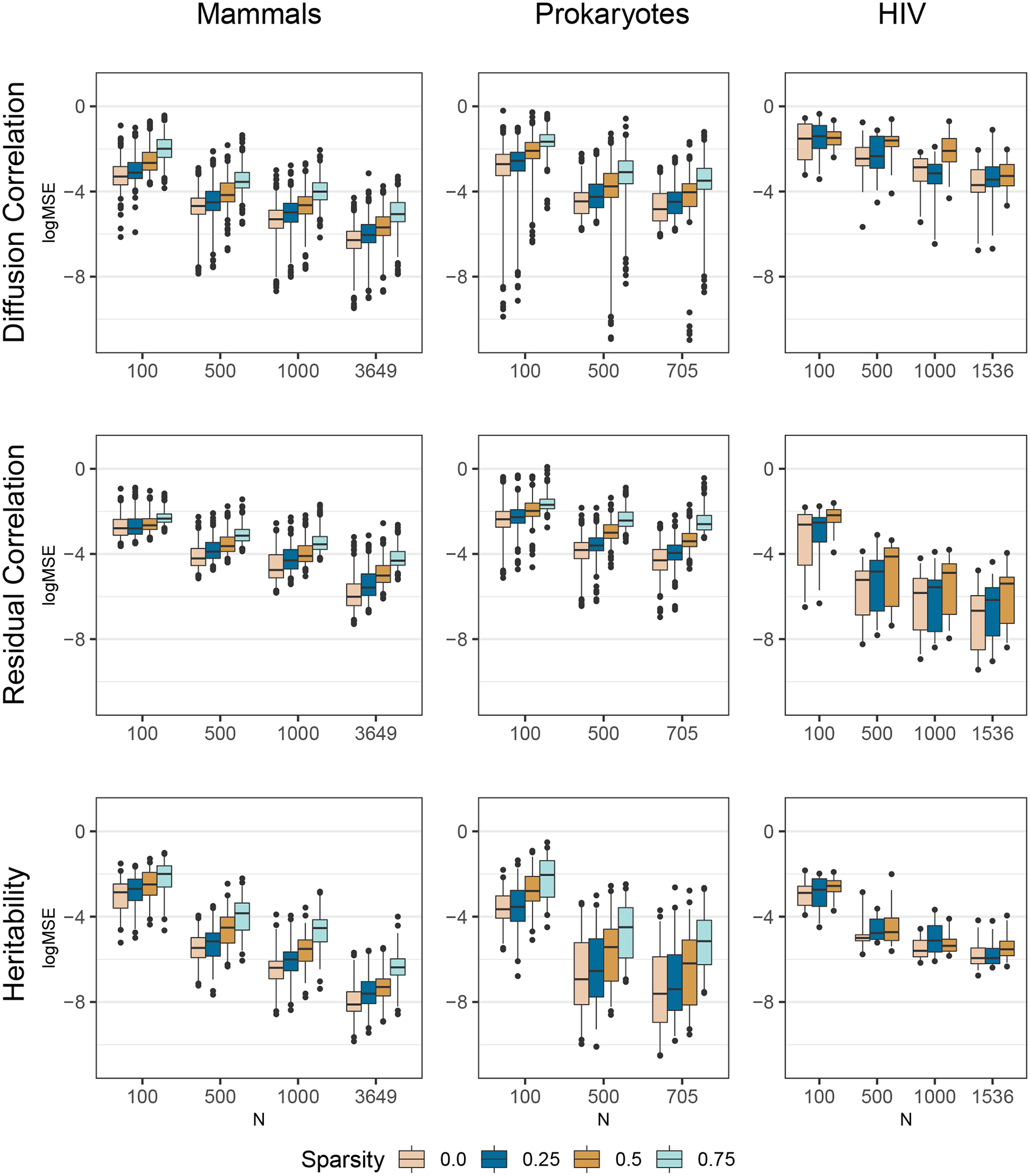
Posterior log mean squared-error of the diffusion correlation, residual correlation, and heritability over ten simulated replicates based on three empirical examples. The boxes extend from the 25^th to the 75^th posterior percentiles with the middle bar representing the median. The lines extend from the 2.5^th through the 97.5^th percentiles, with outliers depicted as dots. The sparsity depicted by different colors represents different percentages of randomly removed data.

7. APPLICATIONS

7.1. Mammalian Life History

A major task for life history theory is to understand the ecological and evolutionary significance of correlation between life history traits such as age at sexual maturity, the number of offspring per reproductive event, and reproductive lifespan (Roff 2002). Establishing patterns of such correlation grants insight into whether life history variation between individuals, populations or species is consistent with pace-of-life theory (Reynolds 2003; Réale et al. 2010). This theory predicts that ‘fast’ traits such as early maturity, large broods, small offspring, frequent reproduction and a short lifespan are positively associated with each other as a consequence of organisms pursuing strategies that prioritize either current or future reproduction. Existing approaches using comparative life history data to investigate fast-slow trait covariation patterns (e.g. mammals: Bielby et al. 2007; hymenoptera: Blackburn 1991; lizards: Clobert et al. 1998; birds: Sæther and Bakke 2000; plants: Salguro-Gómez 2017; fish: Wiedmann et al. 2014) generally support the fast-slow hypothesis; however, results are rarely consistent across taxa. This may reflect important taxonomic differences in life history evolution, but there is concern that differences are an artifact of different methodologies (Jeschke and Kokko 2009).

One key limitation is that previous methods have required complete data for each species. As complete measurements across a rich suite of varied life history traits are not yet available for most species, this means that researchers must choose to either reduce the number of traits or reduce the number of species included in analyses. By integrating out missing traits, we resolve this issue and analyze the life history dataset used in Capellini et al. (2015), which is based largely on the final PanTHERIA dataset (Jones et al. 2009), supplemented with measurements from Ernest (2003) and additional sources. Our analysis includes all the variables analyzed by Bielby et al. (2007) (gestation length, weaning age, neonatal body mass, litter size, litter frequency, and age at first birth) plus reproductive lifespan (maximum lifespan minus age at first birth). We include female body mass as a trait rather than analyze size-corrected residuals and log-transform and standardize all traits prior to analysis. The analysis assumes the phylogeny of Fritz et al. (2009) that remains the most complete phylogeny for mammals. In total, 3649 species in the phylogeny have measurement of at least one trait and are included. Table 2 reports the number of species with measurements for each trait. Only 136 species have complete data on all 8 traits; thus the ability to include species with partially missing traits enables inclusion of 932% more measurements.

Table 2:

Missing data summary for all three examples.

Data set	Trait	Number observed	Percent missing
Mammals N = 3649	Body mass	3467	5.0%
	Litter size	2477	32.1%
	Gestation length	1359	62.8%
	Weaning age	1161	68.2%
	Litter frequency	888	75.7%
	Neonatal body mass	1083	70.3%
	Age at first birth	444	87.8%
	Reproductive lifespan	348	90.5%
	Total	11227	61.5%
Prokaryotes N = 705	Cell diameter	690	2.1%
	Cell length	657	6.8%
	Genome length	563	20.1%
	GC content	563	20.1%
	Coding sequence length	558	20.9%
	Optimal temperature	548	22.3%
	Optimal pH	487	30.9%
	Total	4066	17.6%
HIV N = 1536	GSVL	1536	0.0%
	SPVL	1536	0.0%
	CD4 slope	1102	28.3%
	Total	4174	9.4%

To estimate the correlation between these traits throughout mammalian evolution, we jointly model them with an MBD process on the tree with residual variance. In this analysis, we are primarily interested in the correlation between traits during the MBD process on the tree and estimate trait correlations from the marginal posterior of Σ. Figure 3 summarizes these findings. Our results are clearly consistent with the fast-slow trait covariation patterns that pace-of-life theory predicts. The ‘slow’ life history traits (longer gestation, later weaning, larger neonatal body mass, later age at first birth, and longer reproductive lifespan) are all positively correlated with each other and negatively correlated with the two ‘fast’ life history traits (greater litter size and more frequent litters). All correlations are significant (determined by < 5% posterior tail probability) with the notable exception of that between litter size and litter frequency. This apparent lack of correlation may be due to the opposing effects of their joint positive correlation with body mass combined with a trade-off between these two traits that life history theory predicts (Stearns 1989). Nevertheless, our results demonstrate that larger animals tend to have slower life history traits, confirming known patterns and reflecting the central role of body size in life history evolution.

Figure 3:

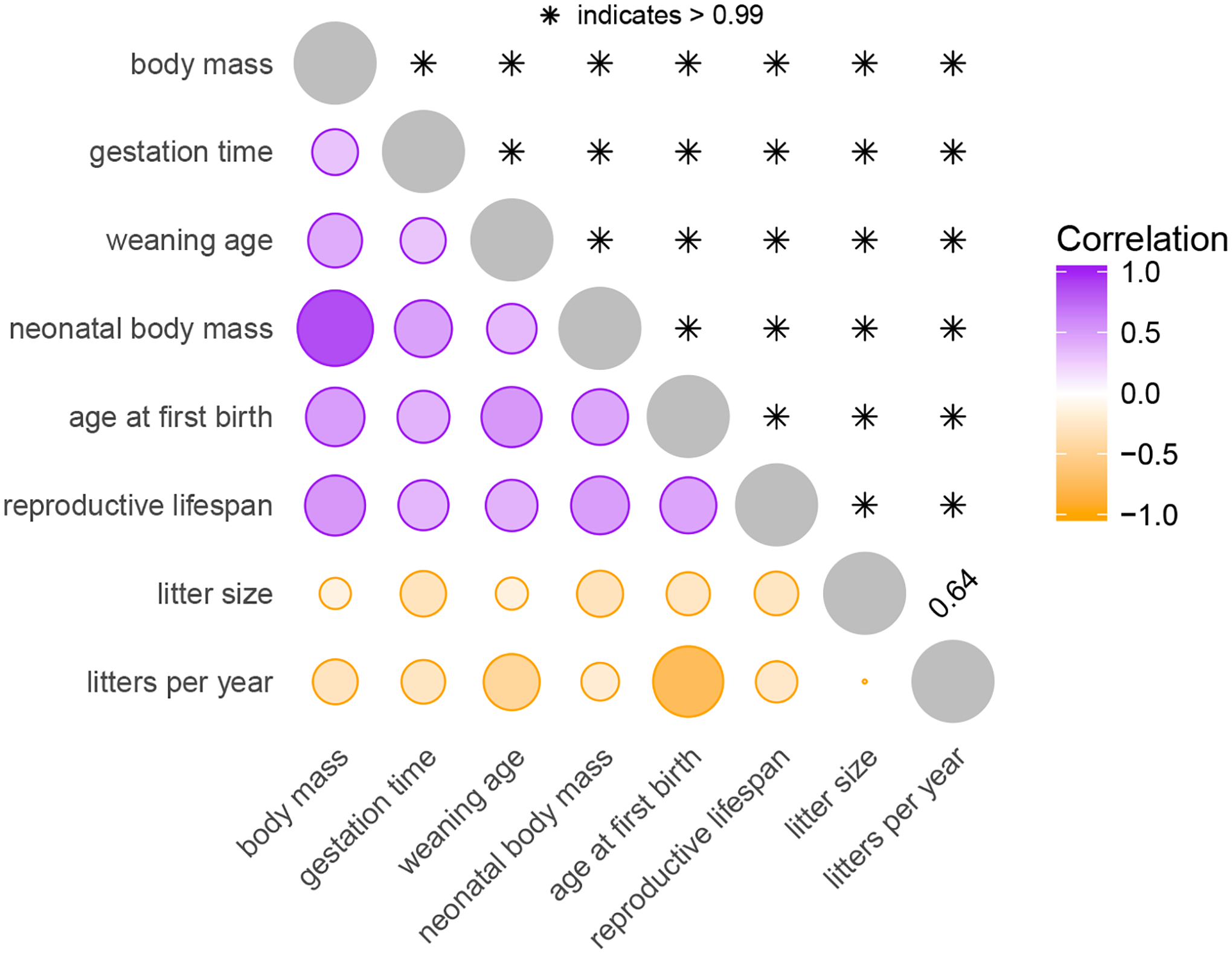
Correlation among mammalian life-history traits. The circles below the diagonal summarize the posterior mean correlation between each pair of traits. Purple represents a positive correlation while orange represents a negative correlation. Circle size and color intensity both represent the absolute value of the correlation. The numbers above the diagonal report the posterior probability that the correlation is of the same sign as its mean.

We compare the computational efficiency of our method against that of the sampling method using the MBD model both with and without residual variance. Table 1 shows an increase in overall computational efficiency of two orders-of-magnitude as indicated by the change in ESS per hour. Additionally, we see that our method succeeds at reducing both the amount of computational work per MCMC sample (as indicated by the increase in samples per hour) and autocorrelation (as indicated by the increase in ESS per sample).

7.2. Prokaryote evolution

Comparative genomics has greatly assisted in the formulation of prokaryote evolutionary theories. Several such theories have been inspired by and tested through measuring correlation among different phenotypic and genomic traits. For example, the thermal adaptation hypothesis posits that higher GC content is involved in adaptation to high temperatures because it may offer thermostability to genetic material (Bernardi and Bernardi 1986). The genome streamlining hypothesis attempts to explain the compactness of prokaryotic genomes through natural selection favoring small genomes (Doolittle and Sapienza 1980; Orgel and Crick 1980; Giovannoni et al. 2014). Sabath et al. (2013) argue that lower cell volume is an adaptive response to high temperature. The field is well-aware of the need to account for phylogenetic relationships when measuring correlation, but statistical analyses generally rely on fixed, poorly resolved trees and simple models of trait evolution.

Here, we estimate correlation among a set of genotypic and phenotypic traits while simultaneously accounting for phylogenetic uncertainty and accommodating complexity in the trait evolutionary process. We construct our data set from a study by Goberna and Verdú (2016), who collated cell diameter, cell length, optimum temperature and pH measurements for a large set of prokaryotes. Prior experience in resolving large, unknown trees suggests that we limit our analysis to less than ~750 taxa. As such, we include all taxa with three or more measurements and a selection of the taxa with only two measurements in our analysis. For our selection of 705 taxa, we obtain data on genome length, the number of coding sequences, and GC content from the prokaryotes table in NCBI Genome. Table 2 presents the number of measurements for each trait. We log-transform and standardize all traits (except for GC content which we logit-transform and standardize). To infer the phylogeny, we obtain matching 16S sequences via the ARB software package (Ludwig et al. 2004) that we then align using the SINA Alignment Service (Pruesse et al. 2012) and manually edit.

Through MCMC simulation, we simultaneously infer the sequence and trait evolutionary process. We model the sequence evolutionary process using a general time-reversible model (Tavaré 1986) with gamma-distributed rate variation among sites (Yang 1994). We use an uncorrelated lognormal relaxed clock to model rate variation among branches (Drummond et al. 2006) and specify a Yule birth prior process on the unknown tree (Gernhard 2008). For the trait evolutionary process, we assume an MBD model with residual variance.

Figure 4 displays our estimated maximum clade credibility phylogeny with associated trait measurements, and Figure 5 presents the phylogenetic correlation between those traits. One notable result is the positive correlation between optimal temperature and GC content (0.22 posterior mean, [0.08, 0.37] 95% highest posterior density interval) that the thermal adaptation hypothesis predicts (Bernardi and Bernardi 1986). Researchers have discussed this hypothesis for years with mixed support (Hurst and Merchant 2001; Musto et al. 2004; Wang et al. 2006; Wu et al. 2012; Sabath et al. 2013; Aptekmann and Nadra 2018). Our analysis, however, includes 435 taxa with measurements for both GC content and optimal growth temperature, making it the largest study we are aware of that accounts for phylogenetic relationships. Interestingly, while cell diameter and cell length are not significantly correlated, they are both positively correlated with genome length. Smaller cells have been associated with smaller genomes in both prokaryotes and unicellular eukaryotes (Shuter et al. 1983; Lynch 2007), but the reasons for this are not fully understood (Dill et al. 2011). We also estimate a relatively strong negative correlation between genome length and optimal temperature (−0.52 [−0.67, −0.37]), supporting the genomic streamlining hypothesis during thermal adaptation. Note that we do not compare computation times here, as simultaneous inference of the phylogenetic tree makes the sampling method prohibitively slow.

Figure 4:

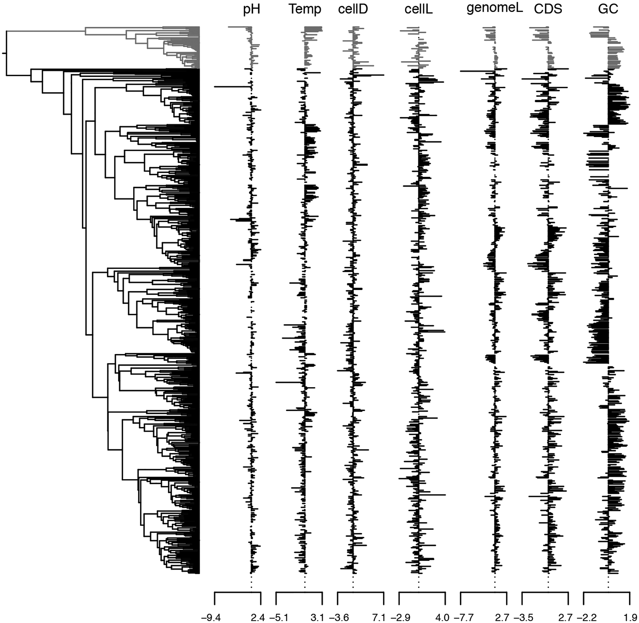
Prokaryote phylogeny and traits. The phylogeny depicts the inferred maximum clade credibility tree. The archaea clade (N = 54) and the associated trait measurements are depicted in grey.

Figure 5:

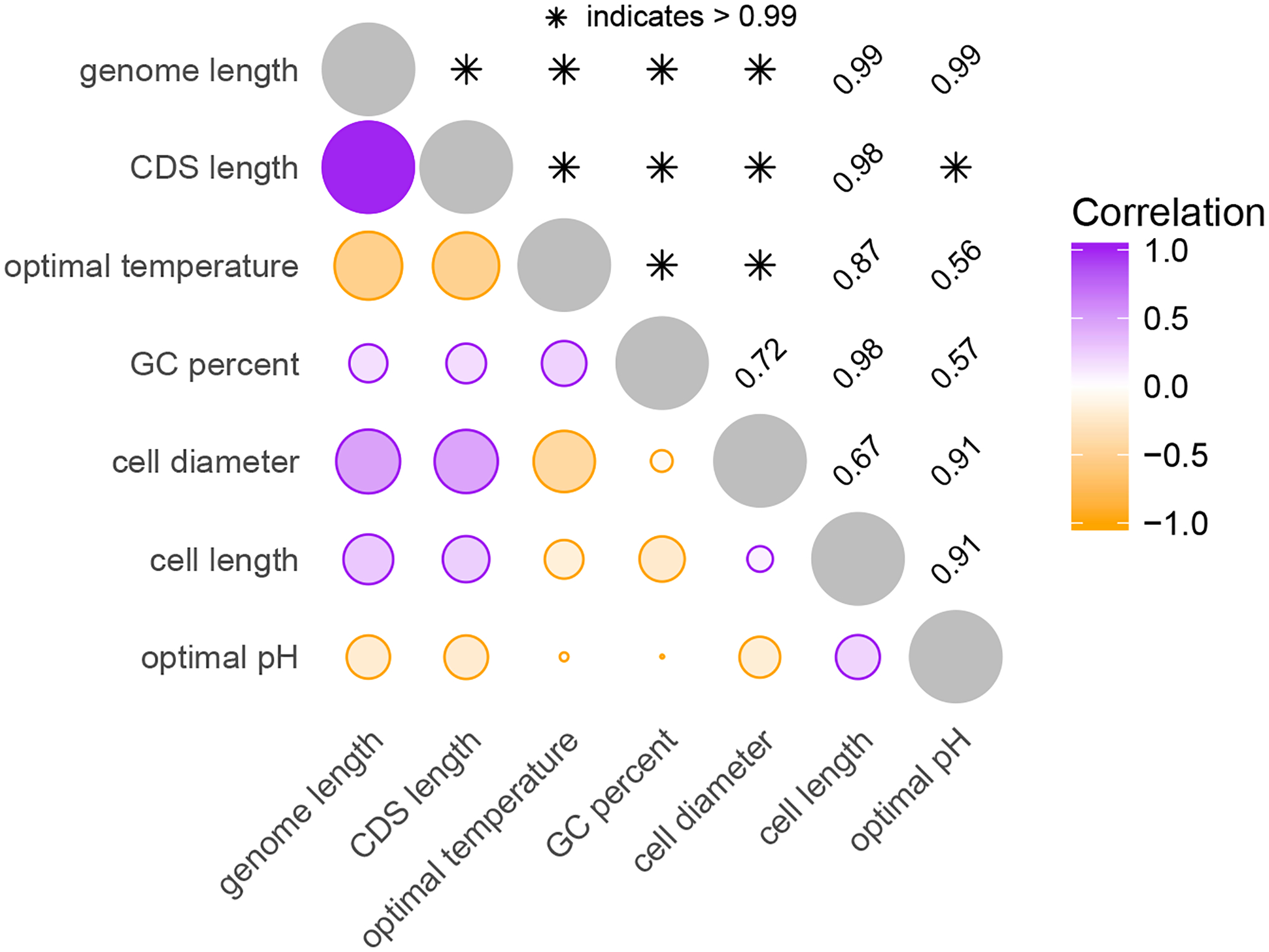
Correlation among prokaryotic growth properties. See Figure 3 caption.

7.3. HIV-1 virulence

Recent years have witnessed a strong interest in using phylogenetic comparative methods to study the heritability of HIV-1 virulence. Initially, Alizon et al. (2010) employed Pagel’s λ (Pagel 1999) to measure the extent to which HIV-1 set-point viral load reflects viral shared evolutionary history in the Swiss HIV Cohort Study (Swiss HIV Cohort Study et al. 2009) patients. A relatively high heritability estimate of set-point viral load, a predictive measure of clinical outcome, motivated others to examine to what extent the viral genotype can control for this trait (e.g. Hodcroft et al. 2014; Vrancken et al. 2015). These efforts have resulted in widely varying estimates, from 6% to 59%, prompting a discussion on the methods used to estimate the heritability of virulence (see Mitov and Stadler 2018; Bertels et al. 2018). Here, we revisit the most comprehensive data set recently analyzed (Blanquart et al. 2017) to determine the extent to which variability in HIV-1 virulence is attributable to viral genetic variation. We focus on the dataset of subtype B viruses from Blanquart et al. (2017) that encompasses 1581 taxa with associated measures of set-point viral load and CD4 cell count decline. We rely on the maximum likelihood phylogeny inferred for this data set, but convert it to a time-measured tree with dated tips using a heuristic procedure (To et al. 2016). A prior examination of the correlation between sampling time and root-to-tip divergence using TempEst (Rambaut et al. 2016) indicated the presence of outliers, most of which can be attributed to a basal lineage in the phylogeny. As the subtyping of the taxa in this basal lineage also was ambiguous (Blanquart, personal communication), we remove this lineage (36 taxa) together with 9 other outlier taxa. We note that this resulted in a time to the most recent common ancestor (TMRCA) estimate of about 1960 that is much more in line with a recent subtype B TMRCA estimate (1967, 95% Bayesian credibility interval of 1963–1970; Worobey et al. 2016) than the estimate including the basal lineage (~1930).

Two measures of set-point viral load are available for all remaining taxa: (i) one based on a standardized choice of assay on a single sample taken between 6 and 24 months after infection and before the initiation of antiretroviral therapy (“gold standard viral load”, GSVL) and (ii) a more classical measure of set-point viral load (SPVL) based on the mean of all log viral loads measured between 6 and 24 months after infection. Figure 6 presents the phylogeny and associated trait values. To estimate heritability of both set-point viral load measures and CD4 slope, we model all three measurements as a multivariate trait in our MBD model with residual variance and approximate the posterior distribution of the heritability statistic H via MCMC. Our estimated heritabilities are 0.21 [0.11, 0.3] for GSVL, 0.18 [0.1, 0.26] for SPVL, and 0.16 [0.07, 0.25] for CD4 cell decline. These estimates are consistent with similar estimates reported by Blanquart et al. (2017).

Figure 6:

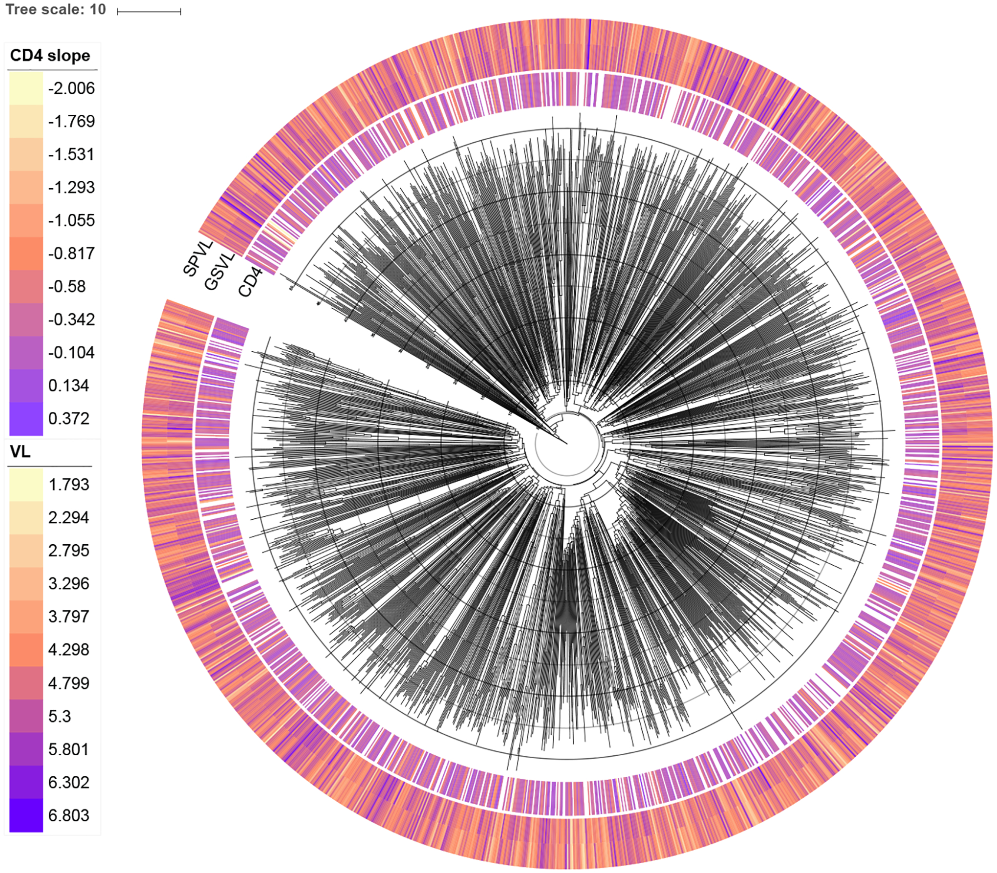
HIV-1 phylogeny with associated CD4 slope, SPVL, and GSVL values for each viral host.

We further asses model fit by assessing predictive performance of GSVL on SPVL. We omit CD4 slope from our analysis as it is measured concurrently with SPVL. We randomly remove 5% of the SPVL measurements from the data set and consider four different models. We consider both a bivariate case where we assume a multivariate process and a univariate case where we analyze SPVL alone. For both the bivariate and univariate cases, we use the MBD model both with and without the residual variance extension. For each removed SPVL measurement, we compute the mean squared error (MSE) between the predicted and true values. We repeat each analysis 50 times and report the cumulative results in Figure 7, from which two results emerge. First, the MSE of prediction in the bivariate cases are lower than those in the univariate cases. This is unsurprising given the strong correlation between SPVL and GSVL. Second, addition of residual variance to the model results in modestly better prediction of SPVL in both the bivariate and univariate cases. This emphasizes the importance of including model extensions like residual variance in these analyses.

Figure 7:

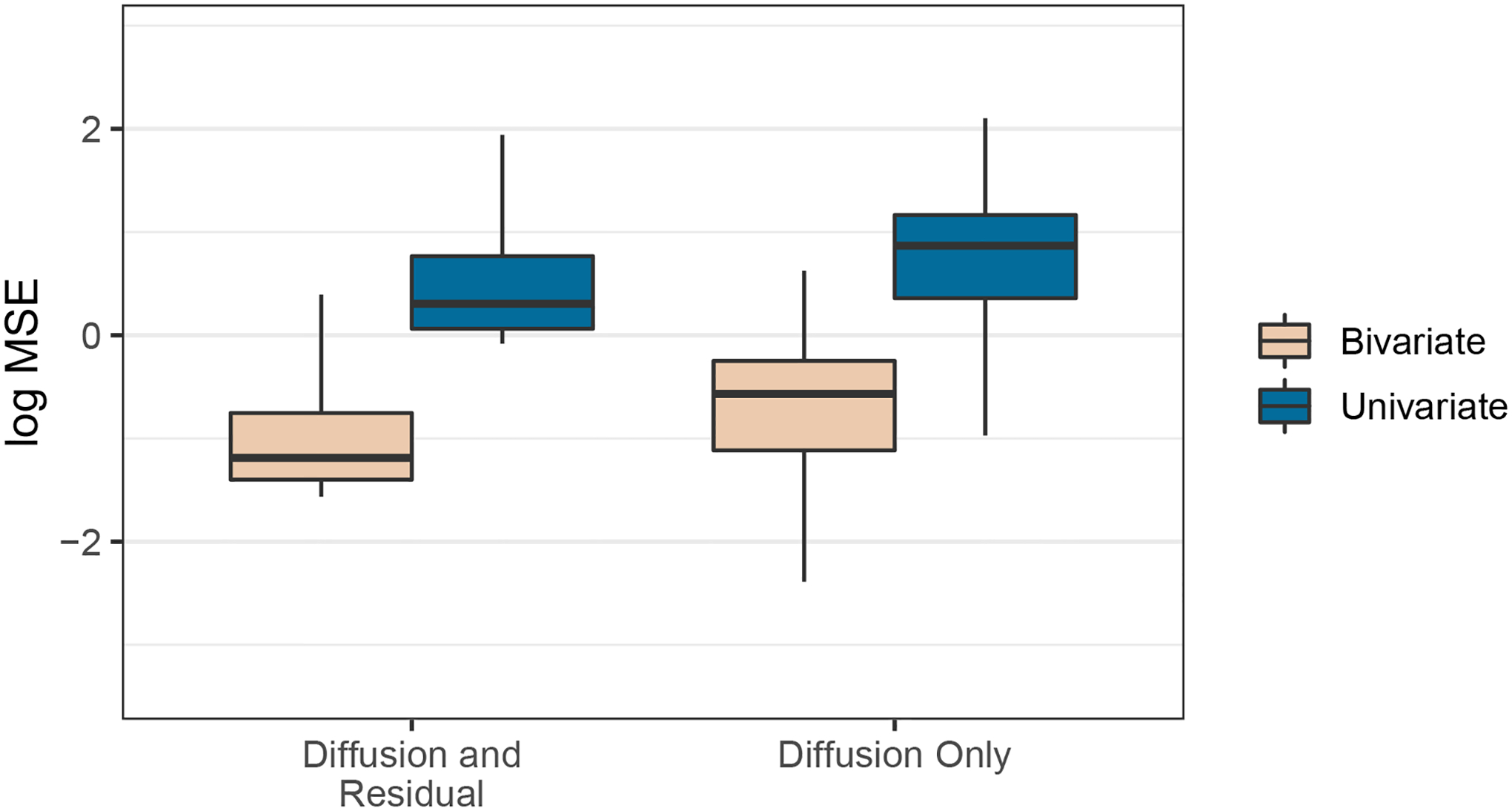
Model predictive performance of HIV set-point viral load. Each box-and-whisker plot depicts the posterior mean-squared-error of prediction under a different model. The boxes represent the interquartile range, while the lines extend to include the 2.5^th through 97.5^th percentiles. Outliers are omitted.

We again demonstrate improvements in computational efficiency (see Table 1). While less dramatic than the mammals example, we still see an order-of-magnitude increase in effective sample size per hour in the MBD model without residual variance. This attenuation is to be expected, as there are far fewer missing measurements in the HIV data set than the mammal data set. Nevertheless, our method still outperforms the sampling method in the simple MBD model even when only 9.4% of data points are missing. For the model with residual variance, our method outperforms the sampling method by two orders-of-magnitude.

8. DISCUSSION

Oftentimes comparative biologists are interested in phylogenetically adjusted methods for assessing relationships between traits of organisms. However, frequently when the number of taxa grows large the level of missing data increases, making inference challenging. Here, we have developed a method for evaluating the likelihood of observed traits given a tree while integrating out missing values analytically that dramatically outperforms current best-practice methods. In the mammalian data set, with N = 3649 and 61.5% missing data, we achieve a minimum effective sample size per hour 400× greater than previous methods. This increase in speed brings computation times down from more than a week to less than an hour. Even in the more tractable HIV data set, with N = 1536 and 9.4% missing data, we increase the minimum ESS per hour by a factor of 65. Both increases in speed are due to an overall decrease in both autocorrelation between MCMC samples and the amount of computational work required per sample. Importantly, this increase in computational efficiency allows for previously intractable analyses on large trees. Specifically, we incorporate residual variance into the model and (in the prokaryotes example) simultaneously infer Σ, Γ, and an unknown phylogeny $\mathcal{F}$. Further, the residual variance extension is only one of several potential extensions. Other possible extensions could incorporate data sets with repeated measurements at the tips of the tree and factor analyses (Tolkoff et al. 2017).

Additionally, our strategy could be used in a more diverse array of phylogenetic models than the fixed-rate MBD process. Recently, Fisher et al. (2020) have used our method in a scale-mixture of multivariate normals diffusion model where there is a different evolutionary rate on each of the tree branches. This model assumes that the rate of evolution changes over time and across taxa. Moreover, these methods also easily translate to multi-optima Ornstein–Uhlenbeck (OU) diffusions, where there is some (potentially changing) optimum trait value that traits tend to evolve toward. Following from Bastide et al. (2018), a modified version of our method has already been implemented for the OU process in BEAST.

We also note that our pre-order missing data augmentation algorithm presented in Section 2.2.1 has far broader utility than computing the conjugate Wishart statistics. Notably, it allows for joint sampling of all missing values in linear-time. As such, this data augmentation procedure serves as a bridge between any data set with missing data and statistical methods that require complete data. Such cases occur, for example, in computing the residual sum of squares in phylogenetic mixed models (Lynch 1991) as well as the gradient of the log likelihood with respect to the model parameters.

An important limitation of our and previous methods is that they assume an ignorable missing data mechanism (i.e. that the data are missing at random and that the prior on any model parameters is independent of the missing data mechanism). Note that this is assumption is not as restrictive as it seems as we only require that the data are missing and random and not necessarily missing completely at random (Little and Rubin 1987). While these conditions may hold in some comparative biology examples, possible violations abound. Any solution to this problem would necessarily depend on the specific missing data mechanism. One commonly used missing data mechanism is the thresholding model where data above or below some limit are omitted from the analysis. This could occur, for example, when there is some minimum detection limit below which a value cannot be measured. To explicitly account for these omissions, we could modify our model to assume the observed data at the tips are drawn from a truncated multivariate-normal distribution rather than a full multivariate normal distribution. Under this model, the observed data likelihood would remain the same up to a normalizing constant and indicator function. As the distribution of the internal nodes would remain un-truncated and the Gaussian kernel on all nodes would remain unchanged, our likelihood calculation algorithm would remain largely unchanged. For the likelihood computation, the normalizing constants and indicator functions would simply be propagated up the tree in the same way as the integration remainders r_i. One challenge of this approach would be to compute the normalizing constants for all taxa with missing data. This may be particularly challenging as, depending on the specific missing data mechanism, these constants may depend on the latent trait values immediately internal to the tip nodes. An additional challenge to this approach would be to formalize the distribution of the missing data so that we could appropriately apply our pre-order data augmentation algorithm. We may simply be able to draw each missing value from their un-truncated full conditional distribution, but more work would be necessary to determine whether this augmentation regime is appropriate. We leave these challenges as future work.

Finally, and perhaps most importantly, we propose our method as a special case solution to the long-standing statistical problem involving multivariate normal distributions with missing data. Specifically, our method applies to any MVN distribution with a three-point structured covariance matrix (see Ho and Ané 2014). Intuitively, this condition arises in covariance matrices generated from processes that are additive on an acyclic graph (see Figure 8). This restriction, however, is not overly limiting and applies to a broad range of normal models including multilevel hierarchical models and matrix-normal distributions such as the one we use here. Additionally, our pre-order data augmentation procedure enables $\mathcal{O}(N)$ imputation in these highly structured models. While Allen and Tibshirani (2010) and Glanz and Carvalho (2018) have utilized the EM algorithm (Dempster et al. 1977) to efficiently perform maximum likelihood imputation in similar problems, our method could serve as an alternative for approaches that base inference on the observed-data likelihood.

Figure 8:

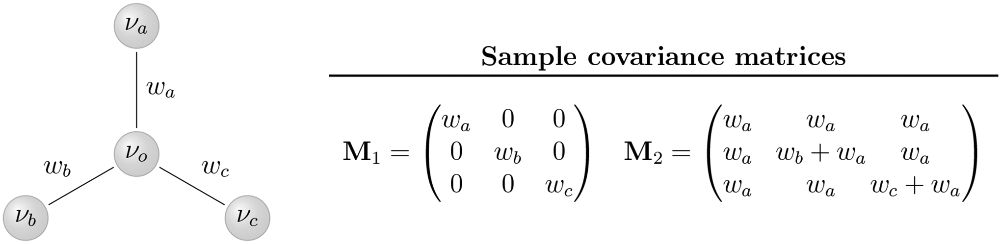
An acyclic graph with nodes {ν_o, ν_a, ν_b, ν_c} and edge weights {w_a, w_b, w_c}. The covariance matrix Λ = {Λ_ij} is additive on an acyclic graph if each Λ_ij is equal to the sum of the shared non-negative edge-weights in the paths from ν_i and ν_j to some origin node. For example, the matrix M₁ is additive for nodes (ν_a, ν_b, ν_c)^t with ν_o at the origin, while the matrix M₂ is additive for nodes (ν_o, ν_b, ν_c)^t with ν_a at the origin.

Bibliography

- Adams DC (2014). A method for assessing phylogenetic least squares models for shape and other high-dimensional multivariate data. Evolution 68(9), 2675–2688. [DOI] [PubMed] [Google Scholar]
- Alizon S, von Wyl V, Stadler T, Kouyos RD, Yerly S, Hirschel B, Böni J, Shah C, Klimkait T, Furrer H, Rauch A, Vernazza PL, Bernasconi E, Battegay M, Bürgisser P, Telenti A, Günthard HF, Bonhoeffer S, and Swiss HIV Cohort Study (2010, Sep). Phylogenetic approach reveals that virus genotype largely determines HIV set-point viral load. PLoS Pathogens 6(9), e1001123. [DOI] [PMC free article] [PubMed] [Google Scholar]
- Allen G and Tibshirani R (2010). Transposable regularized covariance models with an application to missing data imputation. Annals of Applied Statistics 4, 764–790. [DOI] [PMC free article] [PubMed] [Google Scholar]
- Aptekmann AA and Nadra AD (2018). Core promoter information content correlates with optimal growth temperature. Scientific Reports 8(1), 1313. [DOI] [PMC free article] [PubMed] [Google Scholar]
- Bastide P, Ané C, Robin S, and Mariadassou M (2018). Inference of adaptive shifts for multivariate correlated traits. Systematic Biology 67(4), 662–680. [DOI] [PubMed] [Google Scholar]
- Bernardi G and Bernardi G (1986). Compositional constraints and genome evolution. Journal of Molecular Evolution 24(1–2), 1–11. [DOI] [PubMed] [Google Scholar]
- Bertels F, Marzel A, Leventhal G, Mitov V, Fellay J, Günthard HF, Böni J, Yerly S, Klimkait T, Aubert V, Battegay M, Rauch A, Cavassini M, Calmy A, Bernasconi E, Schmid P, Scherrer AU, Müller V, Bonhoeffer S, Kouyos R, Regoes RR, and Swiss HIV Cohort Study (2018, Jan). Dissecting HIV virulence: Heritability of setpoint viral load, CD4+ T-cell decline, and per-parasite pathogenicity. Molecular Biology and Evolution 35(1), 27–37. [DOI] [PMC free article] [PubMed] [Google Scholar]
- Bielby J, Mace G, Bininda-Emonds O, Cardillo M, Gittleman J, Jones K, Orme C, and Purvis A (2007). The fast-slow continuum in mammalian life history: An empirical reevaluation. The American Naturalist 169(6), 748–757. [DOI] [PubMed] [Google Scholar]
- Blackburn T (1991). Evidence for a ‘fast-slow’ continuum of life-history traits among parasitoid Hymenoptera. Functional Ecology 5(1), 65–74. [Google Scholar]
- Blanquart F, Wymant C, Cornelissen M, Gall A, Bakker M, Bezemer D, Hall M, Hillebregt M, Ong SH, Albert J, Bannert N, Fellay J, Fransen K, Gourlay AJ, Grabowski MK, Gunsenheimer-Bartmeyer B, Günthard HF, Kivelä P, Kouyos R, Laeyendecker O, Liitsola K, Meyer L, Porter K, Ristola M, van Sighem A, Vanham G, Berkhout B, Kellam P, Reiss P, Fraser C, and collaboration B (2017, June). Viral genetic variation accounts for a third of variability in HIV-1 set-point viral load in europe. PLoS Biology 15(6), 1–26. [DOI] [PMC free article] [PubMed] [Google Scholar]
- Cantet RJ, Birchmeier AN, and Steibel JP (2004). Full conjugate analysis of normal multiple traits with missing records using a generalized inverted Wishart distribution. Genetics, Selection and Evolution 36, 49–64. [DOI] [PMC free article] [PubMed] [Google Scholar]
- Capellini I, Baker J, Allen W, Street S, and Vendetti C (2015). The role of life history traits in mammalian invasion success. Ecology Letters 18, 1099–1107. [DOI] [PMC free article] [PubMed] [Google Scholar]
- Clobert J, Garland T, and Barbault R (1998). The evolution of demographic tactics in lizards: A test of some hypotheses concerning life history evolution. Journal of Evolutionary Biology 11(3), 329–364. [Google Scholar]
- Cybis G, Sinsheimer J, Bedford T, Mather A, Lemey P, and Suchard M (2015). Assessing phenotypic correlation through the multivariate phylogenetic latent liability model. Annals of Applied Statistics 9, 969 – 991. [DOI] [PMC free article] [PubMed] [Google Scholar]
- Dempster AP, Laird NM, and Rubin DB (1977). Maximum likelihood from incomplete data via the EM algorithm. Journal of the royal statistical society, series B 39(1), 1–38. [Google Scholar]
- Dill KA, Ghosh K, and Schmit JD (2011). Physical limits of cells and proteomes. Proceedings of the National Academy of Sciences 108(44), 17876–17882. [DOI] [PMC free article] [PubMed] [Google Scholar]
- Dominici F, Parmigiani G, and Clyde M (2000). Conjugate analysis of multivariate normal data with incomplete observations. Canadian Journal of Statistics 28, 533–550. [Google Scholar]
- Doolittle WF and Sapienza C (1980). Selfish genes, the phenotype paradigm and genome evolution. Nature 284(5757), 601. [DOI] [PubMed] [Google Scholar]
- Drummond AJ, Ho SY, Phillips MJ, and Rambaut A (2006). Relaxed phylogenetics and dating with confidence. PLoS Biology 4(5), e88. [DOI] [PMC free article] [PubMed] [Google Scholar]
- Ernest S (2003). Life history characteristics of placental nonvolant mammals. Ecology 84(12), 3402. [Google Scholar]
- Falconer DS (1960). Introduction to Quantitative Genetics. Oliver And Boyd; Edinburgh; London. [Google Scholar]
- Fisher AA, Ji X, Zhang Z, Lemey P, and Suchard MA (2020). Relaxed random walks at scale. Systematic Biology 70(2), 258–267. [DOI] [PMC free article] [PubMed] [Google Scholar]
- Freckleton RP (2012). Fast likelihood calculations for comparative analyses. Methods in Ecology and Evolution 3(5), 940–947. [Google Scholar]
- Fritz S, Bininda-Edmonds O, and Purvis A (2009). Geographical variation in predictors of mammalian extinction risk: big is bad, but only in the tropics. Ecology Letters 12(6), 538–549. [DOI] [PubMed] [Google Scholar]
- Gernhard T (2008). The conditioned reconstructed process. Journal of Theoretical Biology 253(4), 769–778. [DOI] [PubMed] [Google Scholar]
- Giovannoni SJ, Thrash JC, and Temperton B (2014). Implications of streamlining theory for microbial ecology. The ISME Journal 8(8), 1553. [DOI] [PMC free article] [PubMed] [Google Scholar]
- Glanz H and Carvalho L (2018). An expectation-maximization algorithm for the matrix normal distribution with an application in remote sensing. Journal of Multivariate Analysis 167, 31–48. [Google Scholar]
- Goberna M and Verdú M (2016). Predicting microbial traits with phylogenies. The ISME Journal 10(4), 959. [DOI] [PMC free article] [PubMed] [Google Scholar]
- Goolsby EW (2017). Rapid maximum likelihood ancestral state reconstruction of continuous characters: A rerooting-free algorithm. Ecology and Evolution 7(8), 2791–2797. [DOI] [PMC free article] [PubMed] [Google Scholar]
- Goolsby EW, Bruggeman J, and Ané C (2017). Rphylopars: fast multivariate phylogenetic comparative methods for missing data and within-species variation. Methods in Ecology and Evolution 8(1), 22–27. [Google Scholar]
- Ho LST and Ané C (2014). A linear-time algorithm for Gaussian and non-Gaussian trait evolution models. Systematic Biology 63(3), 397–408. [DOI] [PubMed] [Google Scholar]
- Hodcroft E, Hadfield JD, Fearnhill E, Phillips A, Dunn D, O’Shea S, Pillay D, Leigh Brown AJ, UK HIV Drug Resistance Database, and UK CHIC Study (2014). The contribution of viral genotype to plasma viral set-point in HIV infection. PLoS Pathogens 10(5), e1004112. [DOI] [PMC free article] [PubMed] [Google Scholar]
- Hurst LD and Merchant AR (2001). High guanine–cytosine content is not an adaptation to high temperature: a comparative analysis amongst prokaryotes. Proceedings of the Royal Society of London B: Biological Sciences 268(1466), 493–497. [DOI] [PMC free article] [PubMed] [Google Scholar]
- Jeschke J and Kokko H (2009). The roles of body size and phylogeny in fast and slow life histories. Evolutionary Ecology 23(6), 867–878. [Google Scholar]
- Jones KE, Bielby J, Cardillo M, Fritz SA, O’Dell J, Orme C, Safi K, Sechrest W, Boakes EH, Carbone C, Connolly C, Cuttis MJ, Foster JK, Grenyer R, Habib M, Plaster CA, Price SA, Rigby EA, Rist J, Teacher A, Bininda-Emonds OR, Gittleman JL, Mace GM, and Purvis A (2009). PanTHERIA: a species-level database of life history, ecology, and geography of extant and recently extinct mammals. Ecology 90(9), 2648. [Google Scholar]
- Little R and Rubin D (1987). Statistical Analysis With Missing Data. Wiley Series in Probability and Statistics - Applied Probability and Statistics Section Series. Wiley. [Google Scholar]
- Liu JS, Wong WH, and Kong A (1995). Covariance structure and convergence rate of the Gibbs sampler with various scans. Journal of the Royal Statistical Society. Series B (Methodological) 57(1), 157–169. [Google Scholar]
- Ludwig W, Strunk O, Westram R, Richter L, Meier H, Yadhukumar, Buchner A, Lai T, Steppi S, Jobb G, et al. (2004). ARB: a software environment for sequence data. Nucleic Acids Research 32(4), 1363–1371. [DOI] [PMC free article] [PubMed] [Google Scholar]
- Lynch M (1991). Methods for the analysis of comparative data in evolutionary biology. Evolution 45(5), 1065–1080. [DOI] [PubMed] [Google Scholar]
- Lynch M (2007). The frailty of adaptive hypotheses for the origins of organismal complexity. Proceedings of the National Academy of Sciences 104(suppl 1), 8597–8604. [DOI] [PMC free article] [PubMed] [Google Scholar]
- Mitov V, Bartoszek K, Asimomitis G, and Stadler T (2020). Fast likelihood calculation for multivariate Gaussian phylogenetic models with shifts. Theoretical Population Biology 131, 66–78. [DOI] [PubMed] [Google Scholar]
- Mitov V, Bartoszek K, and Stadler T (2019). Automatic generation of evolutionary hypotheses using mixed Gaussian phylogenetic models. Proceedings of the National Academy of Sciences 116(34), 16921–16926. [DOI] [PMC free article] [PubMed] [Google Scholar]
- Mitov V and Stadler T (2018). A practical guide to estimating the heritability of pathogen traits. Molecular Biology and Evolution 35(3), 756–772. [DOI] [PMC free article] [PubMed] [Google Scholar]
- Musto H, Naya H, Zavala A, Romero H, Alvarez-Valín F, and Bernadi G (2004). Correlations between genomic GC levels and optimal growth temperatures in prokaryotes. FEBS letters 573(1–3), 73–77. [DOI] [PubMed] [Google Scholar]
- Nakagawa S and Freckleton RP (2008). Missing inaction: the dangers of ignoring missing data. Trends in Ecology & Evolution 23(11), 592–596. [DOI] [PubMed] [Google Scholar]
- Orgel LE and Crick FH (1980). Selfish DNA: the ultimate parasite. Nature 284(5757), 604. [DOI] [PubMed] [Google Scholar]
- Pagel M (1999, October). Inferring the historical patterns of biological evolution. Nature 401, 877–884. [DOI] [PubMed] [Google Scholar]
- Pruesse E, Peplies J, and Glöckner FO (2012). SINA: accurate high-throughput multiple sequence alignment of ribosomal RNA genes. Bioinformatics 28(14), 1823–1829. [DOI] [PMC free article] [PubMed] [Google Scholar]
- Pybus OG, Suchard MA, Lemey P, Bernardin FJ, Rambaut A, Crawford FW, Gray RR, Arinaminpathy N, Stramer SL, Busch MP, and Delwart EL (2012). Unifying the spatial epidemiology and molecular evolution of emerging epidemics. Procedings of the National Academy of Sciences 109(37), 15066–15071. [DOI] [PMC free article] [PubMed] [Google Scholar]
- Rambaut A, Lam TT, Max Carvalho L, and Pybus OG (2016). Exploring the temporal structure of heterochronous sequences using TempEst (formerly Path-O-Gen). Virus Evolution 2(1), vew007. [DOI] [PMC free article] [PubMed] [Google Scholar]
- Réale D, Garant D, Humphries MM, Bergeron P, Careau V, and Montiglio P-O (2010). Personality and the emergence of the pace-of-life syndrome concept at the population level. Philosophical Transactions of the Royal Society B: Biological Sciences 365(1560), 4051–4063. [DOI] [PMC free article] [PubMed] [Google Scholar]
- Revell LJ (2012). phytools: an R package for phylogenetic comparative biology (and other things). Methods in Ecology and Evolution 3(2), 217–223. [Google Scholar]
- Reynolds J (2003). Life histories and extinction risk. In Blackburn T and Gaston K (Eds.), Macroecology: Concepts and Consequences, pp. 195–217. Oxford: Blackwell Publishing Ltd. [Google Scholar]
- Roff DA (2002). Life History Evolution. Sunderland, Massachusetts. Sinauer Associates. [Google Scholar]
- Sabath N, Ferrada E, Barve A, and Wagner A (2013). Growth temperature and genome size in bacteria are negatively correlated, suggesting genomic streamlining during thermal adaptation. Genome Biology and Evolution 5(5), 966–977. [DOI] [PMC free article] [PubMed] [Google Scholar]
- Sæther B-E and Bakke Ø (2000). Avian life history variation and contribution of demographic traits to the population growth rate. Ecology 81(3), 642–653. [Google Scholar]
- Salguro-Gómez R (2017). Applications of the fast-slow continuum and reproductive strategy framework of plant life histories. New Phytologist 213(3), 1618–1624. [DOI] [PubMed] [Google Scholar]
- Shuter BJ, Thomas J, Taylor WD, and Zimmerman AM (1983). Phenotypic correlates of genomic dna content in unicellular eukaryotes and other cells. The American Naturalist 122(1), 26–44. [Google Scholar]
- Stearns SC (1989). Trade-offs in life-history evolution. Functional Ecology 3(3), 259–268. [Google Scholar]
- Suchard MA, Lemey P, Baele G, Ayres DL, Drummond AJ, and Rambaut A (2018a). Bayesian phylogenetic and phylodynamic data integration using BEAST 1.10. Virus Evolution 4(1), vey016. [DOI] [PMC free article] [PubMed] [Google Scholar]
- Suchard MA, Lemey P, Baele G, Ayres DL, Drummond AJ, and Rambaut A (2018b). Bayesian phylogenetic and phylodynamic data integration using BEAST 1.10. Virus Evolution 4(1), vey016. [DOI] [PMC free article] [PubMed] [Google Scholar]
- Swiss HIV Cohort Study, Schoeni-Affolter F, Ledergerber B, Rickenbach M, Rudin C, Günthard HF, Telenti A, Furrer H, Yerly S, and Francioli P (2009). Cohort profile: the swiss hiv cohort study. International Journal of Epidemiology 39(5), 1179–1189. [DOI] [PubMed] [Google Scholar]
- Tavaré S (1986). Some probabilistic and statistical problems in the analysis of DNA sequences. Lectures on Mathematics in the Life Sciences 17(2), 57–86. [Google Scholar]
- To T-H, Jung M, Lycett S, and Gascuel O (2016, Jan). Fast dating using least-squares criteria and algorithms. Systematic Biology 65(1), 82–97. [DOI] [PMC free article] [PubMed] [Google Scholar]
- Tolkoff MR, Alfaro ME, Baele G, Lemey P, and Suchard MA (2017). Phylogenetic factor analysis. Systematic Biology 67(3), 384–399. [DOI] [PMC free article] [PubMed] [Google Scholar]
- Visscher PM, Hill WG, and Wray NR (2008). Heritability in the genomics era—concepts and misconceptions. Nature Reviews Genetics 9(4), 255. [DOI] [PubMed] [Google Scholar]
- Vrancken B, Lemey P, Rambaut A, Bedford T, Longdon B, Günthard HF, and Suchard MA (2015). Simultaneously estimating evolutionary history and repeated traits phylogenetic signal: applications to viral and host phenotypic evolution. Methods in Ecology and Evolution 6, 67–82. [DOI] [PMC free article] [PubMed] [Google Scholar]
- Wang H-C, Susko E, and Roger AJ (2006). On the correlation between genomic G + C content and optimal growth temperature in prokaryotes: data quality and confounding factors. Biochemical and Biophysical Research Communications 342(3), 681–684. [DOI] [PubMed] [Google Scholar]
- Wiedmann M, Primicerio R, Dolgov A, Ottensen C, and Aschan M (2014). Life history variation in Barents Sea fish: Implications for sensitivity to fishing in a changing environment. Ecology and Evolution 4(18), 3596–3611. [DOI] [PMC free article] [PubMed] [Google Scholar]
- Wilks S (1932). Moments and distributions of estimates of population parameters from fragmentary samples. Annals of Mathematical Statistics 3, 163–195. [Google Scholar]
- Worobey M, Watts TD, McKay RA, Suchard MA, Granade T, Teuwen DE, Koblin BA, Heneine W, Lemey P, and Jaffe HW (2016, November). 1970s and ‘Patient 0’ HIV-1 genomes illuminate early HIV/AIDS history in North America. Nature 539(7627), 98–101. [DOI] [PMC free article] [PubMed] [Google Scholar]
- Wu H, Zhang Z, Hu S, and Yu J (2012). On the molecular mechanism of GC content variation among eubacterial genomes. Biology Direct 7(1), 2. [DOI] [PMC free article] [PubMed] [Google Scholar]
- Yang Z (1994). Maximum likelihood phylogenetic estimation from DNA sequences with variable rates over sites: approximate methods. Journal of Molecular Evolution 39(3), 306–314. [DOI] [PubMed] [Google Scholar]
Associated Data
This section collects any data citations, data availability statements, or supplementary materials included in this article.