

Abstract
Motivation
ChIP-seq detects protein–DNA interactions within chromatin, such as that of chromatin structural components and transcription machinery. ChIP-seq profiles are often noisy and variable across replicates, posing a challenge to the development of effective algorithms to accurately detect differential peaks. Methods have recently been designed for this purpose but sometimes yield conflicting results that are inconsistent with the underlying biology. Most existing algorithms perform well on limited datasets. To improve differential analysis of ChIP-seq, we present a novel Differential analysis method for ChIP-seq based on Limma (DiffChIPL).
Results
DiffChIPL is adaptive to asymmetrical or symmetrical data and can accurately report global differences. We used simulated and real datasets for transcription factors (TFs) and histone modification marks to validate and benchmark our algorithm. DiffChIPL shows superior performance in sensitivity and false positive rate in different simulations and control datasets. DiffChIPL also performs well on real ChIP-seq, CUT&RUN, CUT&Tag and ATAC-seq datasets. DiffChIPL is an accurate and robust method, exhibiting better performance in differential analysis for a variety of applications including TF binding, histone modifications and chromatin accessibility.
Availability and implementation
Supplementary information
Supplementary data are available at Bioinformatics online.
1 Introduction
Chromatin immunoprecipitation and high-throughput DNA sequencing (ChIP-seq) has been widely used in genome-wide detection of protein–DNA interactions, such as for transcription factors (TFs) and histone modifications which have important function in 3D genome organization and gene regulation (Kasowski et al., 2013; Kharchenko et al., 2008). Alternative methods to obtain similar information as ChIP-seq, such as Cleavage under targets and release using nuclease (CUT&RUN) and Cleavage Under Targets and Tagmentation (CUT&Tag), have also become popular because of higher efficiency and lower background noise (Kaya-Okur et al., 2019; Skene et al., 2018). In addition, the assay for transposase-accessible chromatin with sequencing (ATAC-Seq) is an important method to profile chromatin accessibility (Buenrostro et al., 2015). For ChIP-seq, many methods have been developed to call narrow and broad peaks. The most popular methods are SPP (narrow and broad) (Kharchenko et al., 2008), MACS2 (narrow and broad) (Zhang et al., 2008) and SICER (broad) (Zang et al., 2009). These methods can also be applied to CUT&RUN, CUT&Tag, and ATAC-seq data, which are inherently different from ChIP-seq data due to lack of input samples. Within called peak regions, one of the most important downstream analyses is differential peaks analysis (DPA) between different treatments or developmental stages.
There are some existing tools or models for DPA for ChIP-seq, which can be separated into two classes based on whether peak calling is integrated. The first class combines peak calling and DPA into one step, including diffReps (Shen et al., 2013), PePr (Zhang et al., 2014), csaw (Lun and Smyth, 2016) and THOR (Allhoff et al., 2016). The second class performs DPA within given peak regions, such as DiffBind v2 and v3 (Ross-Innes et al., 2012; Stark and Brown, 2011), MAnorm/MAnorm2 (Shao et al., 2012; Tu et al., 2021), ChIPComp (Chen et al., 2015) and ROTS (Faux et al., 2021). In this study, we focus on methods in the second class because of their popularity, and robust algorithms for peak calling already exist, such as MACS2, SPP and SICER. The high variation and noise in ChIP-seq data leads to high false positive rates (FPRs) and/or low sensitivity using current DPA methods (Steinhauser et al., 2016).
The normalization methods for existing differential ChIP-seq algorithms such as TMM (trimmed Mean of M-values) and RLE (relative log expression) are derived from RNA-seq methods. These methods assume that the expression of most genes is unchanged, leading to a bias in differential peak results. LOESS (locally weighted regression) in MA-plot (Taslim et al., 2009) and MAnorm/MAnorm2 assume that common peak regions have similar read densities among different conditions. However, in reality, a predominant gain or loss of peaks can occur for ChIP-seq under specific conditions (Brown et al., 2018; Velasco et al., 2017), and most normalization methods can inadvertently eliminate real differences by forcing symmetry of fold change. Compared to other normalization methods, counts per million (CPM) normalization is more adaptable for comparison between different conditions but may be unable to remove systematic technical differences between two conditions, such as experimental noise and batch effects in different experiments (Goh et al., 2017; Johnson et al., 2007). Therefore, CPM normalization alone is inadequate. In DiffChIPL, we combined CPM normalization with our customized LOESS (Cleveland et al., 1992) in order to surmount these problems.
Another major challenge in differential peak calling is ascertaining true differences especially for low count peaks. We find that the mean-variance trend in ChIP-seq sometimes shows a monotonic increase followed by a monotonic decrease. This trend will lead to many differentially called peaks with low enrichment in limma (Smyth, 2004). voom fits a mean-variance trend and uses the precision weight from the trend as input for the linear model, but it assumes the mean-variance trend is decreasing as the mean normalized counts increase (Law et al., 2014). However, this approach is not appropriate for ChIP-seq because many low count peaks have low variance and are thus called as differential. DESeq2 uses an empirical Bayes procedure to shrink the log fold change toward zero for low count genes (Love et al., 2014). MAnorm2 considers the within-group variance in different groups and normalizes all samples using a hierarchical normalization based on MAnorm, which assumes no global change at common peak regions. MAnorm2 also models the precision weights similarly to voom. The within-group variance and the fitting of the mean-variance curve based on a quadratic function can increase the estimated variance for low count peaks. In DiffChIPL, we approached this problem by adjusting the mean-variance trend by increasing the variance for low normalized count peaks and shrinking the variance using James–Stein estimator (Opgen-Rhein and Strimmer, 2007; Stein, 1956).
Here, we developed a robust DPA method called DiffChIPL based on limma that is applicable to ChIP-seq, CUT&RUN, and CUT&Tag for both narrow and broad chromatin binding profiles as well as ATAC-seq data. To optimize our algorithm, we first compared methods of counting reads in peak regions for IP and input samples. Next, we applied different normalization procedures to three different cases to demonstrate the efficiency of our method. For comparisons, we used datasets with known differential peaks to estimate all methods based on sensitivity, FPR and area under the curve (AUC) score. Furthermore, we benchmarked our method against existing differential analysis methods using ChIP-seq, CUT&RUN, CUT&Tag and ATAC-seq datasets. We used matching RNA-seq data to compare changes in gene expression with that of histone mark or ATAC-seq peaks to estimate performance using the Fisher’s exact test (FET). Finally, we discussed the possible applications and limitations of our method.
2 Materials and methods
2.1 Datasets
We used simulated TFs and histones, 13 ChIP-seq datasets (TFs, histones) (Bag et al., 2021; Kasowski et al., 2013), 4 human CUT&RUN histone datasets (Janssens et al., 2018), 3 CUT&Tag histone datasets (Theisen et al., 2021), 4 ATAC-seq datasets from ENCODE (https://www.encodeproject.org/) and corresponding RNA-seq datasets (Supplementary Table S1). For comparison, we used FET to determine if there is a significant positive correlation between differential peaks and differentially expressed genes based on RNA-seq. Here, the differentially expressed genes are identified using DESeq2 with FDR <0.05 and no fold-change cutoff. The differential peaks are identified with same False Discovery Rate (FDR) threshold which represents the adjusted P-values for all methods.
2.2 Removal of background noise
The main workflow of the DiffChIPL method is shown in Figure 1. First, we count the reads in peak regions. One option is to use the NCIS (normalization of ChIP-seq) method (Liang and Keleş, 2012) to calculate a scaling factor to remove background noise in IP samples given the control (input or IgG) samples. It is important to consider the control samples when the background noise shows high variation in peak regions. NCIS assumes that reads in ChIP-seq samples are composed of signal plus background noise and that a linear relationship exists between the background noise in control and IP samples, respectively. It divides the genome into non-overlapping bins and calculates the optimal ratio of read counts in IP and input by separating the background from signal. NCIS was also applied to CUT&RUN, CUT&Tag in this study. Instead of removing background noise, a second option is to use a simple method to count the reads in IP samples only, which does not consider background noise in peak regions no matter whether the experiment has input/IgG samples as control (e.g. ATAC-seq).
Fig. 1.

DiffChIPL workflow for differential peak analysis of two ChIP-seq groups comparison
2.3 Fitting the mean-variance trend
In limma, a linear model is used to fit the log transformed gene expression counts. The gene-wise residual variance is calculated from the fitted value and observed values. For each gene, the residual variance is assumed to follow approximately a scaled chi-square distribution. We summarized the linear model as follows:
| (1) |
Here, , is the total number of peaks. is the vector of normalized counts of all samples at peak . is the design matrix with dimension of . For example, in a comparison of two groups with two replicates in each condition,
| (2) |
is the unknown coefficient vector of average normalized counts in each group. The residual sample variance (sample is omitted for brevity) is
| (3) |
is the residual degree of freedom. is the residual standard deviation. voom models the mean-variance trend by considering the precision weight for each normalized count based on limma. It concludes that the mean-variance trend monotonically decreases as the RNA-seq mean normalized counts increase. The assumption of mean-variance trend is different from our observation in ChIP-seq histone marks where the mean-variance trend is more like a parabolic shape (Supplementary Fig. S1).
In peak calling, there are often peaks with low enrichment, which cannot be reliably reported by differential analysis given the level of background noise and low enrichment compared to other high signal peaks (Supplementary Fig. S2 and Table S2). However, sometimes the residual variances of these low normalized counts () are low, which can lead to significant differential peak calling in limma because of large fold change and low residual variance (Kadota et al., 2008). Meanwhile, the mean-variance trend first monotonically increases and then monotonically decreases (Supplementary Fig. S1A–K). To make the mean-variance trend monotonically decrease as the mean normalized counts increase, we attempted to correct the mean-variance trend when it increases at low mean normalized counts (Step 3 in Fig. 1). Like Cyber-T methods (Baldi and Long, 2001), we first pooled peaks with similar average normalized counts in each window size to calculate the pooled residual standard deviation (Supplementary Fig. S1). The window size is set to a small value (window size = 0.02). By testing different window sizes, we selected window size = 0.02, which can depict the global mean-variance trend (Supplementary Figs S1 and S3A). We calculated the pooled residual standard deviation in each window by ordering the mean normalized counts, then applied LOESS to fit the mean-pooled residual standard deviation trend (Supplementary Fig. S3B) similar to limma, voom and IBMT (Sartor et al., 2006). When the minimum mean normalized count is larger than the threshold, we do not correct the mean-variance trend. Here we set 2 as the threshold to determine whether performing the fit for virtual residual standard deviation for low normalized counts is needed. Next, we fitted the LOESS line using a piecewise linear model (piecewise.linear() in R) with one change point. Then the change point was used to determine the peaks with low normalized counts (Supplementary Fig. S3C). Finally, we fitted the mean-variance trend on the right side of the change point using an exponential decay curve and used this function to predict the virtual residual standard deviation of low normalized counts, which are on the left side of the change point (Supplementary Fig. S3D). The virtual residual standard deviations are used to replace the raw residual standard deviations to make the overall residual standard deviations decrease as the mean normalized counts increase (Supplementary Fig. S3F).
All mean-variance trend plots are shown in Supplementary Figure S4. Ideally, the residual standard deviations should decrease as the mean normalized counts increase (the last two plots in Supplementary Figure S4). However, when the mean-variance trend is monotonically increasing first and then monotonically decreasing, this results in a parabolic shape (Supplementary Fig. S1A). By fitting a higher variance for the low normalized counts, we can correct the mean-variance trend and avoid calling significantly differential peaks with low normalized counts.
2.4 Shrinking the residual variance using the optimal James–Stein estimator
To improve the overall performance in estimation of residual variance in ChIP-seq, we employed the James–Stein shrinkage rules in ‘shrinkage t’ test on the residual standard deviations to minimize the total risk and single component risk (Opgen-Rhein and Strimmer, 2007) (Step 4 in Fig. 1). Compared to the variance shrinkage of Cui et al. (2005), ‘shrinkage t’ test is more efficient and does not require normal or other distribution. The optimal shrinkage estimator in ‘shrinkage t’ test will shrink the variances to median value, which is more efficient than zero or mean target.
The optimal James–Stein estimator can be summarized as follows:
| (4) |
| (5) |
The residual variances are . We define as the difference between predicted normalized counts and raw normalized counts in sample and peak . The computation of are following formulas.
| (6) |
where , , .
As shown in Supplementary Figure S3E, the shrunken residual standard deviations (orange) are closer to the center of raw residual standard deviation than before shrinkage. Intuitively, if the , all residual variances will be shrunken to . If , there will be no shrinkage. The is determined by . The final residual standard deviations are composed of the virtual residual standard deviation for low normalized count peaks and the shrunken residual standard deviations (Supplementary Fig. S3F).
2.5 Removal of systematic technical differences using customized LOESS
The systematic technical differences in high-throughput sequencing data must be removed to observe true signal (Chen et al., 2015; Shao et al., 2012). These systematic technical differences include experimental noise and batch effects in different experiments (influenced by samples, time, reagent, handlers) (Goh et al., 2017; Johnson et al., 2007). LOESS is a very flexible nonlinear regression method for all kinds of complex processes that uses local weighted polynomial regression (Cleveland et al., 1992). Taslim et al. (2009) used nonlinear LOESS for ChIP-seq normalization, but their normalization produces a globally symmetric MA-plot, which may not reflect true differences. We assume that systematic technical differences positively correlate with the mean normalized counts in peaks.
LOESS was applied on mean normalized counts and log fold change (Taslim et al., 2009). The LOESS on normalized data () can be formed as
| (7) |
| (8) |
| (9) |
where are the mean normalized counts in treatment and control samples in peak . is the fitted fold change. is the mean normalized count of peak . is the fold change.
To avoid symmetrical normalization for the MA-plot, we designed a customized LOESS. The main formulas are shown as follows.
| (10) |
| (11) |
| (12) |
| (13) |
| (14) |
The weight is normalized by the maximum value of to make it scale to 1. The weight will reduce the contribution of these points, which have small mean counts for local linear regression and produce a robust fit. is the fold change after subtracting the LOESS curve. is the weighted fold change after adding an offset value . is the raw weighted fold change. Our goal is to find an optimal offset value that can minimize .
| (15) |
The final corrected fold change is
| (16) |
This means the offset value is added to fold change to produce a global shift. In contrast to MAnorm2 and ChIPComp, we do not need to assume common peak regions for normalization. After subtracting the fitting line from raw fold change, the MA-plot becomes symmetrical, and the systematic technical difference and some biological differences will be removed. To recover the biological difference, we calculate an optimal offset value that minimizes the difference between the raw and recovered (Step 6 in Fig. 1 and Supplementary Figure S5).
2.6 Moderated t-test in limma
limma is a method for differential gene expression analysis for microarray and RNA-seq datasets. It uses CPM normalization and the empirical Bayes method to estimate the posterior variance for small samples. Finally, the moderated t-statistic is used to derive the P-value to call the significant differences between two groups.
After obtaining the corrected parameters, we used the moderated t-test in limma to call differential peaks (Step 7 in Fig. 1). The t-statistic in limma is inferred from a hierarchical model. It shrinks the observed variances toward the prior value with prior degree of freedom. With the Bayes posterior variances , the moderated t-test is defined by
| (17) |
is the fold change of average expression level between two experimental conditions. is the weight with default value 1.
3 Results
3.1 Main workflow of DiffChIPL
The main workflow of the DiffChIPL method is shown in Figure 1. With the peak files in configuration files, we first merge these peak files by default. Then we count the reads in IP (and input) samples given the peak regions. Users can remove the background noise by applying the NCIS method on the raw bam files to calculate the scaling factor between IP and input samples. Raw read counts in IP and input samples, read counts after removing background noise, total library size, scaling factors of IP and input samples are extracted after counting the reads (Step 1). Then we use CPM for normalization with total library size (Step 2). With the linear regression on the values, we can obtain the residual variance and mean normalized value for each peak. If the mean-variance trend first monotonically increases, and then monotonically decreases, we correct the mean-variance trend to make it monotonically decrease. To correct the residual variance, we used a windows-based method to pool peaks with similar mean values and calculate the mean residual variance in each window (window size = 0.02 by default, Supplementary Fig. S1). Next, we used LOESS to fit the pooled residual variance and mean normalized counts to get the curve of mean-variance. Then we can determine the change point in the mean-variance curve (Supplementary Fig. S3C) based on piecewise linear model. The values below the change point are the low normalized counts. We fit virtual residual standard deviations for these low normalized counts based on extending the trend on the right side of the change point (Step 3, Supplementary Fig. S3D). To improve the overall performance of variance estimation, we applied the James–Stein estimator (Opgen-Rhein and Strimmer, 2007) on the residual standard deviations (Supplementary Fig. S3E). Then we merge the virtual residual standard deviations of low normalized counts and the shrunken residual standard deviations on the right side of the change point together as the new residual standard deviations (Step 5, Supplementary Fig. S3F). To correct the CPM normalization, we used a customized LOESS on the fold change and mean values to remove the systematic technical differences between two groups (Step 6, Supplementary Figure S5). Finally, with the corrected residual variances and normalization, we applied the moderated t-test in limma to call the differential peaks (Step 7). The mean-variance plots and MA-plots of main comparisons are shown in Supplementary Figure S4 and S6.
3.2 Optimization of read counting methods for implementation in DiffChIPL
For differential analysis, the first step is to count the reads in peak regions. For ChIP-seq datasets, there are IP samples plus matched input/IgG control to determine the background noise. For CUT&RUN and CUT&Tag samples, there is no input, but there is often a parallel IgG control sample that can be used to assess background noise. For ATAC-seq, there are no input or IgG samples. Different counting methods are used in current differential peak analysis methods. MAnorm2 only counts the IP samples. DiffBind uses the total library size or reads in peaks (RiP) to calculate the scaling factor for the input sample and then subtracts the reads in input samples for each peak. The NCIS method separates the background and signal regions to calculate the optimal scaling factor for input to remove the background noise (Liang and Keleş, 2012). We tested three potential counting methods to estimate their performance in DPA for implementation in DiffChIPL. We define the read counting method using IP samples only as ‘No scaling’, the read counting method in DiffBind as ‘Scaling by total library size’, and the NCIS method as ‘Scaling by background library size’.
We tested how these three different counting methods affect the DPA performance of DiffChIPL on three well-defined Drosophila M1BP TF datasets with known expectations by measuring FPR and sensitivity (Fig. 2). For M1BP mock versus M1BP KD, all peaks are expected to be decreased because the target protein is depleted. For M1BP mock1 versus mock2, no differential peaks are expected because these are biological replicate samples. For M1BP sim1 versus sim2, 237 peaks are decreased, and 237 peaks are increased by simulated down sampling of reads (see Supplementary File). The ‘No scaling’ method shows the best performance overall. ‘Scaling by background library size’ method shows slightly lower FPR and lower sensitivity in M1BP mock1 versus mock2 and M1BP sim1 versus sim2 than the ‘No scaling’ method (Fig. 2B and C). High performance of the ‘No scaling’ method was unexpected but may be a result of low background noise in M1BP experiments. The scaling methods result in decreased counts after removing background noise in peak regions, but when background signals in control samples are high, it may be advisable to remove background noise to reduce FPR. ‘Scaling by background library size’ shows better performance than ‘Scaling by total library size’ in sensitivity and FPR overall on these datasets (Fig. 2A–C). Hence, we only further considered use of ‘No scaling’ (DiffChIPL-IP) and ‘Scaling by background library size’ (DiffChIPL-NCIS) counting methods for all later comparisons of DiffChIPL to other methods.
Fig. 2.
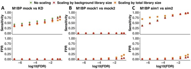
Comparison of DPA performance of DiffChIPL using different reads counting methods on M1BP datasets. (A) M1BP mock versus knockdown. (B) Compare the M1BP mock1 versus mock2. (C) M1BP sim1 versus sim2. Sensitivity and FPR are calculated based on different FDR thresholds (from 1e−7 to 0.1). Here, ‘No scaling’ means only using IP samples to count the reads in the peak regions (IP only). ‘Scaling by background library size’ means to count the reads based using the NCIS method, which calculates the scaling factor between IP and input samples based on the reads in background regions. ‘Scaling by total library size’ means to count reads using the scaling factor, which is calculated from the total library size in IP and input samples. In the ‘Scaling by background library size’ and ‘Scaling by total library size’, the final read counts are subtracting the reads in input samples from IP samples.
3.3 Optimization of normalization methods for implementation in DiffChIPL
The normalization process in ChIP-seq differential analysis is a key step that will greatly affect the final differential peak number between two conditions. We thus compared four different normalization methods (CPM, MAnorm2, TMM, and CPM + customized LOESS) using the read counts from the NCIS method implemented in DiffChIPL based on the three different comparisons of M1BP described above. We used the NCIS method (DiffChIPL-NCIS), which can remove background noise, for these normalization comparisons.
Both TMM and MAnorm2 normalization methods result in overall global symmetry in each of the three cases (Fig. 3A–C). However, for M1BP mock versus knockdown (KD) in which the target protein is depleted, most peaks should only be decreased, not increased, so global symmetry should not be observed (Fig. 3A). In contrast, CPM normalization with or without customized LOESS correction results in mainly decreased peaks for M1BP mock versus knockdown. Furthermore, when considering M1BP mock versus mock comparison (Fig. 3B), CPM with customized LOESS correction results in a more symmetrical distribution of effects compared to CPM alone. Finally, CPM with customized LOESS correction also performs closer to expectation than CPM alone for the M1BP simulation data (Fig. 3C). In summary, CPM with customized LOESS correction can remove most systematic technical differences and can be applied in all cases without losing global real differences.
Fig. 3.

Comparison of four normalization methods on M1BP transcription factor data. (A) M1BP mock versus M1BP KD where most peaks should be decreased. (B) M1BP mock1 versus M1BP mock2, where most peaks should not be changed. (C) Simulation M1BP mock1 versus M1BP mock2, where the overall increased and decreased peaks should be similar. The points above the dotted line are peaks for which fold change >0, and the points below the dotted line are peaks for which fold change <0. Here, MAnorm2 and TMM only work well for results presented in columns 2 and 3. CPM only works well for column 1. ‘CPM + customized LOESS’ correction is applicable in all three cases.
3.4 DiffChIPL outperforms alternative methods for differential peak analysis
To examine the performance of DiffChIPL in differential peak calling compared to other existing methods, we quantified the sensitivity, FPR and AUC score using the three M1BP comparisons as well as simulation human histone modification data generated using csaw. We performed 10 different comparisons in each condition in Figure 4A–D (see details in Supplementary File) (FDR < 0.05). For M1BP mock versus KD, we only calculated the sensitivity because all peaks are decreased (FDR < 0.05). For M1BP mock1 versus mock2, we only calculated the FPR based on selected differential peaks because no differential peaks are expected. For M1BP and histone simulation, we calculated the AUC score based on the FDR and sensitivity for each comparison.
Fig. 4.
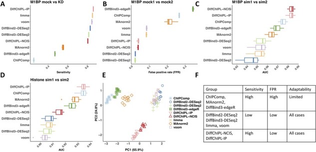
Comparison of the performance of all methods with respect to sensitivity, FPR and AUC scores. (A) The sensitivity of all methods under FDR <0.05 for 10 comparisons of Drosophila M1BP mock versus knockdown (KD). (B) The false positive rate (FPR) of all methods under FDR <0.05 for 10 comparisons of Drosophila M1BP mock1 versus mock2. (C) The AUC score for 10 comparisons of transcription factor M1BP sim1 versus sim2. (D) The AUC scores for 10 comparisons of simulation histone sim1 versus sim2. (E) Principal component analysis plot for all methods based on the four scores in A–D. The optimal cluster number is 3 determined by k-means clustering and within cluster sums of squares using fviz_nbclust() in R. (F) Summary of the features of all methods based on A–E. For ChIPComp, we used pvalue.wald. All methods are ranked based on mean value for 10 comparisons. DiffChIPL-IP only uses the read counts from IP samples. DiffChIPL uses read counts with background noise removed based on the NCIS methods. limma and voom also used NCIS read counting. DiffBind3-edgeR uses TMM normalization in A–E. DiffBind3-DESeq2 uses the DBA_NORM_LIB normalization.
We tested DiffChIPL using both read counting methods (-IP and -NCIS). The limma and voom methods were also run using NCIS read counting. We found that DiffChIPL-IP shows higher sensitivity than other methods, and DiffChIPL-NCIS ranks in the middle for sensitivity. For M1BP mock1 versus mock2 (Fig. 4B), DiffChIPL-NCIS and DiffChIPL-IP also display low FPR (<0.05). For TF simulation (Fig. 4C), DiffChIPL-NCIS and DiffChIPL-IP show higher AUC and less variance than other methods. In Figure 4D, DiffChIPL-IP shows the highest AUC. DiffChIPL-NCIS is ranked in the middle for AUC score.
With the scores in Figure 4A–D as features, we performed principal component analysis on all 40 comparisons. These methods are classified into three groups based on k-means clustering and within cluster sums of squares using fviz_nbclust() in R. (Fig. 4E). By combining the comparisons in Figure 4A–D, we summarized the properties of the three groups into a table in Figure 4F. In Group 1, these methods show high sensitivity and high FPR. In Group 2, these methods can control the FPR but their sensitivity is relatively low (Fig. 4C and D). In Group 3, DiffChIPL-NCIS and DiffChIPL-IP show high sensitivity (Fig. 4A, C and D) and can also display low FPR (Fig. 4B), which distinguish them from the other groups. Due to the normalization method for Groups 2 and 3 being based on total library size (Fig. 4F), their adaptability is good for all cases. In summary, DiffChIPL-NCIS and DiffChIPL-IP can improve the sensitivity and reduce FPR in ChIP-seq differential analysis.
3.5 DiffChIPL shows superior performance in calling differential peaks on mammalian datasets
We next estimated the performance of DiffChIPL compared to other methods based on FET using human histone modification marks and mouse ATAC-seq datasets. The active chromatin state marks H3K4me2 and H3K4me3 are positively correlated with gene expression when overlapping with gene promoters (Janssens et al., 2018). The active chromatin mark H3K36me3 is positively correlated with gene expression when overlapping with gene body (Kundaje et al., 2015). The active chromatin marks H3K4me1 and H3K27ac correspond to enhancers that are typically located within 50 kb of transcription start sites of active genes (Jiang and Mortazavi, 2018). When the repressive mark H3K27me3 overlaps with gene promoters, its presence is anti-correlated with gene expression (Jiang and Mortazavi, 2018; Kundaje et al., 2015; Zhou et al., 2011). Finally, ATAC-seq peaks that overlap with gene promoters are positively correlated with gene expression (Tu et al., 2021).
FET is used to calculate the odds ratio, which reflects the association between the differential peaks and differential genes (see Section 2) for each set of comparisons. In each plot, the methods are ranked based on the mean odds ratio for all comparison sets. Different FDR thresholds are used to determine differential peaks for all methods (Fig. 5, Supplementary Figs S7–S9). When FDR <0.1, FDR <0.05 and FDR <0.01, DiffChIPL-NCIS and DiffChIPL-IP are top ranked in most cases (Fig. 5, Supplementary Figs S7 and S8). Only for H3K36me3, DiffChIPL-NCIS and DiffChIPL-IP are ranked last (Fig. 5, Supplementary Figs S7 and S8). When FDR <0.001, DiffChIPL-NCIS and DiffChIPL-IP is ranked as first to fourth in four cases, respectively, and fifth and seventh for H3K36me3, respectively (Fig. 5, Supplementary Fig. S9). DiffChIPL shows globally higher performance in most cases except for the H3K36me3 ChIP-seq.
Fig. 5.

Comparison of performance of all methods on (A) ChIP-seq H3K4me3, (B) ChIP-seq H3K36me3, (C) CUT&RUN, (D) CUT&Tag and (E) ATAC-seq datasets using FET test. For ChIP-Seq H3K4me3, H3K36me3 and ATAC-seq datasets, there are six separate comparisons shown using each analysis method. There are four comparisons for CUT&RUN and three comparisons for CUT&Tag datasets. For ATAC-seq, the FET value of ChIPComp is not shown because input samples cannot be provided for differential analysis. Some methods detected zero differential peaks, and these FET values are not shown
We selected five examples to illustrate the performance of DiffChIPL. For H3K4me3 GM12890 versus GM12891 (Fig. 5A), there are ∼33 k decreased peaks and 16 k increased peaks using either limma or voom analysis. Most peaks show decreased signals. DiffChIPL-NCIS, DiffChIPL-IP and DiffBind2 also show similar patterns. DiffBind3, MAnorm2 and ChIPcomp show symmetrical MA-plots in which the increased and decreased peaks are about 22∼27 k. Below FDR <0.05, the odds ratio of DiffChIPL-NCIS is highest. From the MA-plot (Supplementary Fig. S10), DiffChIPL-NCIS avoids differential peaks with low mean normalized counts compared to limma and voom. In addition, the peak number of DiffChIPL-NCIS is approximately <50% of other methods (Supplementary Fig. S15). DiffChIPL-IP is ranked below DiffChIPL-NCIS, and their MA-plots are similar.
For H3K36me3 GM12890 versus GM12891 (Fig. 5B), limma, voom, DiffChIPL-NCIS, DiffChIPL-IP and DiffBind2 show similar increased (4∼5 k) and decreased (15∼17 k) peak numbers. ChIPComp, MAnorm2 and Diffbind3-edgeR show more symmetrical MA-plots with similar peak numbers for increased (7∼9 k) and decreased peaks (11∼13 k) (Supplementary Fig. S11). The number of differential peaks for DiffChIPL-NCIS is smaller than limma and voom after removing the differential peaks with low mean normalized counts (Supplementary Figures S11 and S15). However, the odds ratio of limma and voom are much higher than DiffChIPL-NCIS and DiffChIPL-IP. These results indicate that the differential peaks with low mean normalized counts overlap with the differential genes in RNA-seq. Different from other comparisons, H3K36me3 peak overlaps are based on whole gene body, which is more complex than promoter regions and can easily be affected by gene length.
For CUT&RUN H3K4me3 H1 versus K562 (Fig. 5C), the odds ratio of DiffChIPL-NCIS and DiffChIPL-IP are 2.5 and 2.4, respectively, which are larger than voom (∼1.7) and other methods (∼1) under FDR <0.05. The MA-plots show an overall symmetric pattern for increased and decreased peaks (Supplementary Fig. S12). The proportion of overlapping peaks between DiffChIPL and other methods is larger than 90% (Supplementary Fig. S15).
Compared to other datasets, there is very high variation (Supplementary Fig. S4) in CUT&Tag datasets due to the low correlation between replicates. In the CUT&Tag H3K27ac wtEF versus A673 (Fig. 5D), the odds ratio of DiffChIPL-NCIS and DiffChIPL-IP are 7.36 and 0.78, which is larger than other methods (<0.7) except DiffBind3-DESeq2-LIB (∼1.2) under FDR <0.05. The MA-plots show an overall symmetric pattern for increased and decreased peaks (Supplementary Fig. S13). For limma and voom, no differential peaks are called due to high variance. Except for ChIPComp, other methods called hundreds of differential peaks under FDR <0.05. DiffChIPL can call some differential peaks due to the shrinkage of variance. Compared to DiffChIPL-IP, DiffChIPL-NCIS called more differential peaks than DiffChIPL-IP, despite background noise removal.
For ATAC-seq datasets, there are no input samples, so we only tested DiffChIPL-IP. In Figure 5E, we compared the chromatin accessibility difference in forebrain and midbrain tissues. The odds ratio of DiffChIPL-IP is 1.7, which is smaller than DiffBind3-DEseq2 (LIB) (∼2.1) under FDR <0.05. From the MA-plot, most peaks are decreased (Supplementary Fig. S14). For ATAC-seq datasets, DiffChIPL-IP shows overall higher performance than other methods in all six comparisons among forebrain, hindbrain, midbrain and heart. From the five examples, we find that DiffChIPL-IP and DiffChIPL-NCIS called similar numbers of differential peaks on histone datasets. They display overall higher odds ratios than other methods except for H3K36me3 datasets.
4 Discussion
We developed a new method DiffChIPL for differential peak analysis based on limma that displays overall better performance for simulation and real datasets including ChIP-seq, CUT&RUN, CUT&Tag and ATAC-seq datasets. Based on CPM normalization and customized LOESS correction, DiffChIPL is adaptive to asymmetrical or symmetrical normalization cases for DPA without dependence of common peaks in two conditions, and it can also accurately report global differences. Using James–Stein shrinkage, the variances are shrunken toward the median value of whole variances, which can avoid extreme variance and achieve better performance (Supplementary Fig. S16). Finally, we used the moderated t-test in limma to calculate the P-value for peaks. DiffChIPL can achieve both a low FPR and high sensitivity. The FET results of DiffChIPL show that the differential peaks are more associated with the differential RNA-seq genes compared to other methods except for the H3K36me3 datasets. In summary, DiffChIPL is not only applicable for differential analysis of TF binding and histone modifications with both narrow and broad peaks (ChIP-Seq, CUT&RUN, CUT&Tag), it also shows higher performance in differential analysis of chromatin accessibility (ATAC-seq).
It is important to determine how background noise in ChIP-Seq affects the differential analysis performance. DiffChIPL provides two ways to count reads in peak regions including the NCIS method, which can remove the background noise in IP samples paired with input samples, and an IP method to count the reads with IP samples only without removing background noise. We first showed that the IP and NCIS methods are two potential read counting methods in DPA. With real and simulation datasets, we calculated the background noise ratio between IP and input samples and the total library size ratio between IP and input samples. We found that CUT&Tag datasets show the lowest noise levels, and CUT&RUN also displays low noise levels compared to ChIP-seq (Supplementary Fig. S17). Based on the background noise ratio, we simulated TF and histone modification for three background noise levels. DiffChIPL-IP shows significantly better performance for low background noise levels in both TF and histone simulations (Supplementary Fig. S18). For middle and high background noise levels, DiffChIPL-IP and DiffChIPL-NCIS show close performance levels (Supplementary Fig. S18). These results suggest that the NCIS method is helpful to remove the effect of background noise. DiffChIPL-IP is applicable for all background noise level datasets, and DiffChIPL-NCIS is an option when encountering middle or high background noise level datasets. Based on the results in Figure 4B and C, DiffChIPL-NCIS shows slightly higher sensitivity and lower FPR than DiffChIPL-IP on M1BP datasets. Users can use DiffChIPL-NCIS on TF binding datasets when they prefer more conservative results.
For the DiffChIPL method, we can only compare two groups at this time, but the method could be extended to multiple group comparisons in the future. The changing point to distinguish the low normalized count peaks is determined by fitting the outline of mean-variance trend within a given window size. DiffChIPL selects an empirical window size, which is small enough and can also depict the global mean-variance trend. Hence, a more adaptive method may be used to determine the optimal window size. For normalization, DiffChIPL applies customized LOESS correction on fold change. It does not calculate the scaling factor for each sample and is not capable of variance correction. A hierarchical method like MAnorm2 may be potentially applied to normalize each sample. Finally, DiffChIPL is implemented in R. Read counting of bam files will require more processing time than MAnorm2, and DiffChIPL-NCIS takes more time than DiffChIPL-IP when calculating the background noise level.
Supplementary Material
Acknowledgements
We thank Ming-An Sun, Weiqun Peng, Yunhao Wang, Kun Zhu and members of the Lei Lab for discussion and/or comments on the manuscript.
Funding
This work was supported by the Intramural Program of the National Institute of Diabetes and Digestive and Kidney Diseases, National Institutes of Health [DK015602 to E.P.L.].
Conflict of Interest: none declared.
Contributor Information
Yang Chen, Nuclear Organization and Gene Expression Section, Laboratory of Biochemistry and Genetics, National Institute of Diabetes and Digestive and Kidney Diseases (NIDDK), National Institutes of Health (NIH), Bethesda, MD, USA.
Shue Chen, Nuclear Organization and Gene Expression Section, Laboratory of Biochemistry and Genetics, National Institute of Diabetes and Digestive and Kidney Diseases (NIDDK), National Institutes of Health (NIH), Bethesda, MD, USA.
Elissa P Lei, Nuclear Organization and Gene Expression Section, Laboratory of Biochemistry and Genetics, National Institute of Diabetes and Digestive and Kidney Diseases (NIDDK), National Institutes of Health (NIH), Bethesda, MD, USA.
References
- Allhoff M. et al. (2016) Differential peak calling of ChIP-seq signals with replicates with THOR. Nucleic Acids Res., 44, 1–14. [DOI] [PMC free article] [PubMed] [Google Scholar]
- Bag I. et al. (2021) M1BP cooperates with CP190 to activate transcription at TAD borders and promote chromatin insulator activity. Nat. Commun., 12, 1–18. [DOI] [PMC free article] [PubMed] [Google Scholar]
- Baldi P., Long A.D. (2001) A Bayesian framework for the analysis of microarray expression data: regularized t-test and statistical inferences of gene changes. Bioinformatics, 17, 509–519. [DOI] [PubMed] [Google Scholar]
- Brown J.L. et al. (2018) Global changes of H3K27me3 domains and Polycomb group protein distribution in the absence of recruiters Spps or Pho. Proc. Natl. Acad. Sci. USA, 115, 1839–1848. [DOI] [PMC free article] [PubMed] [Google Scholar]
- Buenrostro J.D. et al. (2015) ATAC‐seq: a method for assaying chromatin accessibility genome‐wide. Curr. Protoc. Mol. Biol., 109, 1, 21–29. [DOI] [PMC free article] [PubMed] [Google Scholar]
- Chen L. et al. (2015) A novel statistical method for quantitative comparison of multiple ChIP-seq datasets. Bioinformatics, 31, 1889–1896. [DOI] [PMC free article] [PubMed] [Google Scholar]
- Cleveland W.S. et al. (1992) Local regression models. In: Chambers J.M., Hastie T.J. (eds.) Chapter 8 of Statistical Models in S. Routledge, pp. 309–376. [Google Scholar]
- Cui X. et al. (2005) Improved statistical tests for differential gene expression by shrinking variance components estimates. Biostatistics, 6, 59–75. [DOI] [PubMed] [Google Scholar]
- Faux T. et al. (2021) Differential ATAC-seq and ChIP-seq peak detection using ROTS. NAR Genom. Bioinform., 3, lqab059. [DOI] [PMC free article] [PubMed] [Google Scholar]
- Goh W.W.B. et al. (2017) Why batch effects matter in omics data, and how to avoid them. Trends Biotechnol., 35, 498–507. [DOI] [PubMed] [Google Scholar]
- Janssens D.H. et al. (2018) Automated in situ chromatin profiling efficiently resolves cell types and gene regulatory programs. Epigenetics Chromatin, 11, 1, 1–14. [DOI] [PMC free article] [PubMed] [Google Scholar]
- Jiang S., Mortazavi A. (2018) Integrating ChIP-seq with other functional genomics data. Brief. Funct. Genomics, 17, 104–115. [DOI] [PMC free article] [PubMed] [Google Scholar]
- Johnson W.E. et al. (2007) Adjusting batch effects in microarray expression data using empirical Bayes methods. Biostatistics, 8, 118–127. [DOI] [PubMed] [Google Scholar]
- Kadota K. et al. (2008) A weighted average difference method for detecting differentially expressed genes from microarray data. Algorithms Mol. Biol., 3, 8–12. [DOI] [PMC free article] [PubMed] [Google Scholar]
- Kasowski M. et al. (2013) Extensive variation in chromatin states across humans. Science, 342, 750–752. [DOI] [PMC free article] [PubMed] [Google Scholar]
- Kaya-Okur H.S. et al. (2019) CUT&Tag for efficient epigenomic profiling of small samples and single cells. Nat. Comm., 10, 1–10. [DOI] [PMC free article] [PubMed] [Google Scholar]
- Kharchenko P.V. et al. (2008) Design and analysis of ChIP-seq experiments for DNA-binding proteins. Nat. Biotechnol., 26, 1351–1359. [DOI] [PMC free article] [PubMed] [Google Scholar]
- Kundaje A. et al. ; Roadmap Epigenomics Consortium. (2015) Integrative analysis of 111 reference human epigenomes. Nature, 518, 317–330. [DOI] [PMC free article] [PubMed] [Google Scholar]
- Law C.W. et al. (2014) Voom: precision weights unlock linear model analysis tools for RNA-seq read counts. Genome Biol., 15, R29. [DOI] [PMC free article] [PubMed] [Google Scholar]
- Liang K., Keleş S. (2012) Normalization of ChIP-seq data with control. BMC Bioinformatics, 13, 199–110. [DOI] [PMC free article] [PubMed] [Google Scholar]
- Love M.I. et al. (2014) Moderated estimation of fold change and dispersion for RNA-seq data with DESeq2. Genome Biol., 15, 550–521. [DOI] [PMC free article] [PubMed] [Google Scholar]
- Lun A.T., Smyth G.K. (2016) Csaw: a bioconductor package for differential binding analysis of ChIP-seq data using sliding windows. Nucleic Acids Res., 44, e45. [DOI] [PMC free article] [PubMed] [Google Scholar]
- Opgen-Rhein R., Strimmer K. (2007) Accurate ranking of differentially expressed genes by a distribution-free shrinkage approach. Stat. Appl. Genet. Mol. Biol., 6, 1–8. [DOI] [PubMed] [Google Scholar]
- Ross-Innes C.S. et al. (2012) Differential oestrogen receptor binding is associated with clinical outcome in breast cancer. Nature, 481, 389–393. [DOI] [PMC free article] [PubMed] [Google Scholar]
- Sartor M.A. et al. (2006) Intensity-based hierarchical Bayes method improves testing for differentially expressed genes in microarray experiments. BMC Bioinformatics, 7, 1–17. [DOI] [PMC free article] [PubMed] [Google Scholar]
- Shao Z. et al. (2012) MAnorm: a robust model for quantitative comparison of ChIP-Seq data sets. Genome Biol., 13, 1–17. [DOI] [PMC free article] [PubMed] [Google Scholar]
- Shen L. et al. (2013) diffReps: detecting differential chromatin modification sites from ChIP-seq data with biological replicates. PloS one, 8, 1–13. [DOI] [PMC free article] [PubMed] [Google Scholar]
- Skene P.J. et al. (2018) Targeted in situ genome-wide profiling with high efficiency for low cell numbers. Nat. Protoc., 13, 1006–1019. [DOI] [PubMed] [Google Scholar]
- Smyth G.K. (2004) Linear models and empirical Bayes methods for assessing differential expression in microarray experiments. Stat. Appl. Genet. Mol. Biol., 3, 1–26. [DOI] [PubMed] [Google Scholar]
- Stark R., Brown G. (2011) DiffBind: differential binding analysis of ChIP-Seq peak data. Bioconductor, 1–40.
- Stein C. (1956) Inadmissibility of the usual estimator for the mean of a multivariate normal distribution. In: Neyman J.(Ed.) Proceedings of the Third Berkeley Symposium on Mathematical Statistics and Probability: Contributions to the Theory of Statistics, Vol. 1. University of California Press, pp. 197–206. [Google Scholar]
- Steinhauser S. et al. (2016) A comprehensive comparison of tools for differential ChIP-seq analysis. Brief. Bioinform., 17, 953–966. [DOI] [PMC free article] [PubMed] [Google Scholar]
- Taslim C. et al. (2009) Comparative study on ChIP-seq data: normalization and binding pattern characterization. Bioinformatics, 25, 2334–2340. [DOI] [PMC free article] [PubMed] [Google Scholar]
- Theisen E.R. et al. (2021) Chromatin profiling reveals relocalization of lysine-specific demethylase 1 by an oncogenic fusion protein. Epigenetics, 16, 405–424. [DOI] [PMC free article] [PubMed] [Google Scholar]
- Tu S. et al. (2021) MAnorm2 for quantitatively comparing groups of ChIP-seq samples. Genome Res., 31, 131–145. [DOI] [PMC free article] [PubMed] [Google Scholar]
- Velasco S. et al. (2017) A multi-step transcriptional and chromatin state Cascade underlies motor neuron programming from embryonic stem cells. Cell Stem Cell, 20, 205–217. [DOI] [PMC free article] [PubMed] [Google Scholar]
- Zang C. et al. (2009) A clustering approach for identification of enriched domains from histone modification ChIP-Seq data. Bioinformatics, 25, 1952–1958. [DOI] [PMC free article] [PubMed] [Google Scholar]
- Zhang Y. et al. (2008) Model-based analysis of ChIP-Seq (MACS). Genome Biol., 9, R137–R139. [DOI] [PMC free article] [PubMed] [Google Scholar]
- Zhang Y. et al. (2014) PePr: a peak-calling prioritization pipeline to identify consistent or differential peaks from replicated ChIP-Seq data. Bioinformatics, 30, 2568–2575. [DOI] [PMC free article] [PubMed] [Google Scholar]
- Zhou V.W. et al. (2011) Bernstein. Charting histone modifications and the functional organization of mammalian genomes. Nat. Rev. Genet., 12, 7–18. [DOI] [PubMed] [Google Scholar]
Associated Data
This section collects any data citations, data availability statements, or supplementary materials included in this article.