

Abstract
Adolescent idiopathic scoliosis (AIS) is a three-dimensional curvature of spine. Children with AIS and low bone quality have higher chance to get curve progression leading to bigger spinal curvature. In addition, bone quality affects acoustic impedance of bone, thus influencing the reflection coefficient of ultrasound signal from the soft tissue–bone interface. This study aimed to estimate the bone quality of AIS patients based on the reflection coefficients to determine the correlation of the bone quality with curve severity. A simple bone model was used to develop an equation to calculate the reflection coefficient value. Experiments were conducted on five different phantoms. Acrylic was used to design a vertebral shape to study the effect of surface roughness and inclination, including: smooth flat surface (SFS), smooth curved surface (SCS), rough curved surface (RCS), and the rough curved inclined surface (RCIS). A clinical study with 37 AIS patients were recruited. The estimated reflection coefficient values of plate phantoms agreed well with the predicted values and the maximum error was 6.7%. The reflection coefficients measured from the acrylic-water interface for the SFS, SCS, RCS, RCIS (3° and 5°) were 0.37, 0.33, 0.28, (0.23 and 0.12), respectively. The surface roughness and inclination increased the reflection loss. From the clinical data, the average reflection coefficients for children with AIS were 0.11 and 0.07 for the mild curve group and the moderate curve group, respectively. A moderate linear correlation was found between the reflection coefficients and curve severity ( = 0.3). Patients with lower bone quality have observed to have larger spinal curvature.
Keywords: Adolescent idiopathic scoliosis, ultrasound reflection coefficient, bone quality, curve severity, correlation
Introduction
Scoliosis is a three-dimensional spinal deformity characterized by a lateral curvature of the spine. Adolescent idiopathic scoliosis (AIS) is the most commonly diagnosed form of scoliosis with unknown etiology, 1 affecting 1%–4% adolescent population especially children from 10 to 16 years old.2,3 The severely progressed curves can have negative impact not only on patients’ psychosocial health but also on their physical well-being such as back pain, diminished pulmonary function, and increased mortality rate.4,5 The standard method to measure the severity and monitor the progression of scoliosis is to measure the curvature on the frontal radiograph, which is called the Cobb angle. However, taking radiographs has a significant negative impact on patient well-being. The radiation dose received by a scoliosis patient during radiographic examination has been estimated at between 150 and 678 µSv.6,7 On average, a 10-year-old child who is diagnosed with scoliosis may require 10–22 radiographs during the entire treatment period.8,9 The lifetime risk of radiation is also more pronounced in children than in adults.
From literature, osteopenia or low bone density, quantified by bone mineral density (BMD), is more commonly observed in children with AIS than the normal children.10–13 BMD measures the amount of calcium and is usually tested by dual-energy X-ray absorptiometry (DXA). Furthermore, children with AIS not only have lower BMD, but also have lower bone quality. 14 Bone quality, which is related to bone strength, describes its microarchitecture, mineralization, turnover rate, and micro-fractures. 15 Bone quality can be assessed by radiographic methods. 4 Again, the ionizing radiation exposure to children is a concern. Studies have revealed that the AIS groups have deteriorated bone quality and lower bone mass when compared with the control groups.14,16–19 Lee et al. also found the Cobb angle of scoliosis was inversely and independently associated with BMD. 12 Furthermore, researchers have reported that bone quality could be a risk factor and used to predict the progression of AIS.20–22 Improving children’s bone strength could reduce the risk of curve progression. Treatment management may be provided more effectively if the child has a higher risk of curve progression.
On the other hand, quantitative ultrasound (QUS) is a non-invasive and ionizing radiation-free technique to evaluate bone quality. Lam et al. used the ultrasound transmission-through technique to measure bone properties at calcanei on healthy group as well as both mild and moderate AIS subjects.14,23 Two measured QUS parameters, namely speed of sound (SOS) and broadband ultrasound attenuation (BUA), and the third derived stiffness index (SI), which is a combination of BUA and SOS, were found statistically lower in AIS group than the healthy control group. Further, they suggested that SI was an independent and prognostic factor for curve progression and treatment planning. 23 Similar to the study of finding the relationship between BMD and severity of AIS, 12 Du et al. attempted to correlate SOS with Cobb angles. 24 They found AIS subjects had lower SOS-values compared to non-scoliotic controls; however, they concluded no significant correlation between SOS and Cobb angles. So far, research findings have shown consistently that both bone quantity (BMD) and bone quality (SOS, BUA, and SI) could be found lower in AIS patients as compared to those of normal controls. The findings of low bone quality or BMD in patients with AIS implied that low bone quality could be concurrent with AIS. Studying bone quality in AIS could gain a better understanding of the etiology and bone health in AIS. Furthermore, bone quality was also used as a risk factor to predict progression of AIS,23,24 which could assist in the prevention of curve progression and treatment plans of AIS.12–14 However, a positive correlation between bone quantity or quality and curve severity has not been assertively established yet. In addition, the QUS usually uses transmission method to assess bone quality at peripheral sites other than spines, namely calcaneus and radius.14,24 The use of reflected echoes from spinal scans to evaluate bone quality of the spines is limited.
When ultrasound propagates into the tissue, energy is reflected by any scatter which has a contrast of acoustic impedance with the surrounding, and the strength of the echo mainly depends upon the magnitude of the contrast. Soft tissue–bone interface is an example of strong reflector.25,26 Given that the acoustic impedance of bone, which is a product of SOS and density, is related to the bone stiffness, and thus bone quality. Zheng et al. proposed to measure the ultrasound echoes directly from spines to assess bone quality and correlated with spinal severity of AIS. 27 They introduced a reflection index (RI), which is a ratio of the received echo from the vertebra and a reference echo from a referenced phantom. The results showed that the RI decreased with the increase of curve severity; however, the correlation coefficient was small and the thickness of the soft tissue was ignored. Due to the limited fundamental work and experimental justification in the study of Zheng et al. we would like to develop a framework to explain the fundamental phenomenon of ultrasound echo from spine to assess bone properties.
Therefore, this study aimed to (a) develop the theoretical framework to explore the feasibility of determining reflection coefficients from the ultrasound echoes acquired directly from spines, and (b) investigate if there are correlations between the reflection coefficient with the curve severity in children with AIS.
Materials and methods
Reflection coefficient and bone properties
In this study, the clinical application of the reflection coefficient is to estimate the bone properties of spine. The elastic modulus of cortical bone, E, varies with its density , through . 28 Other forms of the relationship were provided in a review study by Helgason et al. 29 Elasticity is then associated with velocity through , where is the Poisson’s ratio. 30 Changes in bone properties such as density and velocity affect the acoustic impedance of the bone, and thus large reflection coefficient of the soft tissue-bone interface implying better bone quality. From the literature, the density of cortical bone in human ranges from 1800 to 2000 kg/m3,31,32 and correspondingly velocity ranges from 2617 to 3666 m/s,33,34 which corresponds to the impedance range of 4.7–7.3 Mrayls, and thus R-range of 0.49–0.64.
Theoretical formulation
A simple bone model with the cortex overlaid by soft tissue (Figure 1(a)) was used to develop the correlation of the reflection coefficient and the amplitude of the ultrasound signals. Both cortex and soft tissue are assumed to be homogeneous and isotropic. The thickness of soft tissue is while the thickness of cortex is not relevant in this study. The cortical bone and soft tissue are characterized by the velocity ( ), density ( ), and the attenuation coefficient ( ), where the subscripts and are used to denote bone and soft tissue, respectively. The recorded amplitude of the echo can be described by
Figure 1.

(a) A simple bone model with a transducer on top of soft tissue which covers the cortical bone and (b) the primary and multiple reflections within the tissue mimicking layer used to estimate and .
| (1) |
where A0 and A are the amplitudes of the ultrasound source and echo signals, respectively; is the reflection coefficient of the soft tissue–cortex interface, accounts for the attenuation of the signal in the soft-tissue layer, and is the attenuation coefficient of the soft tissue (np/cm). It is noted that we did not consider the signal loss due to spreading with distance because the distance is small in comparison with the width of the transducer.
The relationship between bone properties and the reflection coefficient is expressed as
| (2) |
where and are the acoustic impedances of bone and soft tissue, respectively.
The extraction of in equation (1) requires the knowledge of of the source signal and the attenuation coefficient of the tissue medium. To estimate and in the following phantoms’ study, we utilize the multiple reflections or reverberation within a piece of soft-tissue mimic. Figure 1(b) shows one primary echo and two reverberations within the phantom. The following equations show the correlation of the reflection coefficient, amplitude of reflected signals and the amplitude of the source signal:
| (3) |
where A0, A1, A2, A3 are the magnitude of the source signal, first, second and third reflected signals. The subscripts , , and refer to soft-tissue mimic, acrylic, and matching layer of the transducer respectively; , , and are respectively the attenuation coefficient of the soft-tissue mimic, the reflection coefficients of the soft-tissue mimic–acrylic, and soft-tissue mimic–matching layer interfaces.
By defining
| (4) |
equation (4) can be generalized as
| (5) |
Taking logarithm of both sides linearizes the above equation
| (6) |
where and ln( ) are the slope and intercept of the best fitting line (ln vs ) by linear regression.
Plated phantom study
Experimental setup
The SonixTouch Q+ultrasound system equipped with a 128-element C5-2/60 convex transducer (BK Medical, MA, USA) was employed for the study. The center frequency of the transducer was set at 3.3 MHz for the whole study unless otherwise stated.
Figure 2(a) shows the experimental setup on one of the testing materials, acrylic plate. The transducer was mounted on an aluminum frame and placed in contact with a piece of 2.9-cm thick blue phantom (BP) (CAE Healthcare, FL, USA) overlying an acrylic plate, which was supported by two rubber corks. BP was used because it has ultrasound properties similar to those of soft tissue. Ultrasonic gel (Parker Laboratories, NJ, USA) was applied to all contacting surfaces between the transducer and the BP as well as between the BP and the test plate to ensure good coupling. The thickness of BP after being compressed by the transducer was approximately 2.2 cm. The received RF ultrasound signal was recorded and used to determine the and based on equation (6).
Figure 2.

(a) Experimental setup to measure the ultrasound properties of Blue Phantom and an acrylic plate and (b) experimental setup to measure the reflection from a rough curved surface. The surface is also tilted about 5° around the X axis (in YZ plane).
Reflection coefficient ( ) of five different materials
Various phantoms were used to validate the theory and to study the affecting factors on the ultrasound signals. Based on the previous experimental setup, the acrylic plate was also replaced by different metal plates such as aluminum, brass, copper, and steel to estimate their reflection coefficients with BP. The stiffness of the tested materials ranged from soft to hardest (related to density) while the acoustic impedance of bone should be between that of acrylic and aluminum. Equation (1) was used to determine the reflection coefficient of the five materials based on the measured ultrasound signals.
The determination of theoretical reflection coefficients is based on equation (2) and requires the predetermined densities, velocities, or acoustic impedance. The density of the BP was measured by the Archimedes’ principle while the densities of the five plates were referenced from the literature. The velocities of the used materials, i.e. BP and five plates, were measured by the ultrasonic pulse-echo method using the previous described framework. We obtained the travel time from the RF signals and measured the thicknesses by caliper. The velocity is the ratio between the travel time and the thickness. Regarding the matching layer of the transducer, its acoustic impedance is pooled from reference. 35 These values used for the calculation of reflection coefficients are listed in Table 1.
Table 1.
Properties of the materials used in the study.
| Material | Density (kg/m3) | Velocity (m/s) | Impedance (Mrayls) |
|---|---|---|---|
| Water | 1000 36 | 1480 36 | 1.48 |
| Blue Phantom (BP) | 900 | 1485 | 1.34 |
| Soft tissue | 1050 37 | 1540 38 | 1.62 |
| Cortical bone | 193039–41 | 325039–41 | 6.27 |
| Acrylic | 1180 42 | 2720 | 3.21 |
| Aluminum | 270042,43 | 6150 | 16.61 |
| Brass | 8415 43 | 4275 | 35.97 |
| Copper | 890042,43 | 4515 | 40.18 |
| Steel | 8030 42 | 5700 | 45.77 |
| PZT | – | – | 33.00 35 |
| Matching layer a | – | – | 7.30 b |
Effect of surface roughness and inclination upon the echo-amplitude
Beside the plate study, a 2.4-cm thick acrylic plate with a 19-cm diameter arc on one side (Figure 2(b)) was used to mimic the posterior arch of a vertebra. The surface of the arc was rough, which was caused by the circular-saw cutting. The transducer was placed at 3.5 cm from the rough surface of the phantom, which was similar to a normal distance from an ultrasound transducer to a lamina when the ultrasound was used to scan a scoliotic patient. To investigate the influence of the surface roughness, three scans were performed on (a) a smooth flat surface (SFS), (b) rough curved surface (RCS), and (c) a smooth curved surface (SCS) which was created by sanding the rough curved surface. The phantom at RCS was also tilted at about 3° and 5° in the direction perpendicular to the long axis of the transducer array, named RCIS, to examine the effect of inclination on the recorded echo amplitudes (Figure 2(b)). The experiments were carried out in a water tank with both the transducer and the phantom immersed in water.
Cadaveric vertebral phantom study
A second phantom study was performed on a cadaveric dry lumbar vertebra. The vertebra phantom was fixed to the bottom of the water tank with LePage® Fun-Tak® mounting putty (Lepage, Canada). Similar to the acrylic arch phantom experiment, the vertebra was submerged in water with the transducer set at 3.5 cm from the laminae. Again, the reflection coefficient of the cortical bone surface was calculated using equation (1) with the measured ultrasound signal amplitudes.
In vivo pilot study
The in vivo pilot study was to further validate the proposed approach and to investigate if there was a correlation between the reflection coefficient with the curve severity in children with AIS.
Study participants
Thirty-seven children (9 M; 28 F), aged 14.0 ± 1.6 years old (ranged between 11 and 17), were recruited from the local scoliosis clinic. Ethics approval was obtained from the University of Alberta Health Research Ethics Board (Pro00005707). All participants signed the written consents prior to participation. The inclusion criteria were participants who (1) were diagnosed with AIS, (2) had the age ranging from 10 to 18 years old, (3) had Cobb angle between 10° and 45° (mild to moderate cases), and (4) had no prior surgeries.
Data acquisition
The same ultrasound system described in the phantom study with the convex transducer was used for the in vivo study. The scanning parameters used were: −15 dB power, 6-cm imaging depth, and 50% gain with linear time gain compensation (TGC). These parameters were selected based on the previous studies with some minor adjustments to ensure optimal image quality. 46 Data was obtained by an operator with 2-year experience in using the ultrasound system to scan AIS subjects. The participants were asked to stand in a standard upright posture (Figure 3(a)) within a frame to prevent twisting of the body. The ultrasound gel was applied to their backs prior to scanning. During scanning, the transducer was positioned perpendicular to the coronal profile of the subjects and moved along the spinal curve. Transverse B-mode images (cross-section image of a vertebra) (Figure 3(b)) were displayed in real-time, this allowed the operator to ensure the transducer was almost perpendicular to the lamina region. In this study, we used the low lumbar region (either L4 or L5) for analyses because these two vertebrae usually had little axial rotation in the spinal axis. Approximately 50–100 B-mode images and the corresponding radio-frequency (RF) data were exported for further analysis.
Figure 3.

(a) The ultrasound scan of children with AIS in standing position and (b) a B-mode image of a vertebra. A cadaver vertebra is shown in the inset.
Selection of B-mode frames
The lamina has been identified as a strong ultrasound reflector because the lamina area is usually a relatively flatten surface. 25 This was similar to the arch phantom and the linear plate studies. The middle of the lumbar vertebra L5 was first identified. If the quality of image on L5 was poor, L4 was then used. Five consecutive B-mode frames around the middle of the vertebra with the most leveled pair of laminae were used.
Signal processing for both phantoms and in vivo studies
The acquired RF data was exported by Matlab software (R2019a, MathWorks, MA, USA). Each ultrasound frame had 256 time series (A-lines). Hilbert transform was applied to the series to obtain the envelopes of the signals. 47 The peaks of the envelopes were used as amplitudes to calculate the reflection coefficients. The envelope technique has been shown to be robust in facilitating the detection of the peaks of noisy signals, thereby yielding more consistent and stable results. For the studies of plate phantoms, three records with maximum amplitudes from the center of the transducer were used. In the vertebral phantom and in vivo studies, about3–5 records of maximum echo-magnitudes corresponding to each lamina were exploited to measure the . The measured is the result of averaging the from both laminae.
Results
Phantom studies
Determination of , , and
The primary echo and two reverberations traveling within the BP are shown in Figure 4(a) with the envelope peaks ( ) being 15,863, 2120, and 274, respectively, which were the average of the three time series at locations corresponding to the center of the transducer. By means of equation (4), the are converted to with and from Table 2. The best fitting line goes through the three points (Figure 4(b)) with a close to unity, indicating the perfect fit between the data and the line. The source amplitude, was calculated to be 84,000. The best-fitted is 0.18 np/cm or 1.53 dB/cm, which is compatible to the results obtained by transmission-through measurements with the correction for transmission loss through the water–BP interfaces. 48 The determined thus can be considered the intrinsic absorption coefficient of BP. Figure 4(c) demonstrates the effect of varying (0.3, 0.5, and 0.8 dB/cm/MHz) on the signal amplitude. Further using the echo and multiples, the velocity of the BP ( ) was estimated to be 1485 m/s.
Figure 4.

(a) Envelopes of the recorded echo and two reverberations within the BP. The amplitude of the second reverberation is small and the zoomed signal is shown in the inset. (b) The linear regression line of the three data points. (c) The simulated amplitude ratio with change of soft-tissue thickness for three -values. (d) Comparison between the measured and predicted reflection coefficients. Error bars denote the standard deviations (see Table 2).
Table 2.
The calculated and measured reflection coefficients of the interfaces involved in this study. is given by the absolute value of the difference (calculated – measured) divided by the calculated value.
| Reflection coefficients | Calculated | Measured | (%) |
|---|---|---|---|
| BP/Acrylic ( ) | 0.41 | 0.38 ± 0.02 | 6.68 |
| BP/Aluminum | 0.85 | 0.84 ± 0.06 | 1.60 |
| BP/Brass | 0.93 | 0.94 ± 0.07 | 1.73 |
| BP/Copper | 0.94 | 0.98 ± 0.11 | 4.41 |
| BP/Steel | 0.94 | 0.96 ± 0.02 | 2.14 |
Reflection coefficient ( ) of five different materials
Based on the received reflection signals and equation (1), the measured reflection coefficients, , of the BP–plate interfaces are shown in Table 2. The velocity measurements used for the reference reflection coefficients fall within the ranges provided in literature (Table 1). The discrepancies between the measured and the calculated ranged from 1.60% to 6.68%. Figure 4(d) also shows the measured reflection coefficients versus the calculated for the five plates.
Influence of surface roughness and inclination
Using the signals from the smooth flat surface (SFS) as the reference, the measured from the SFS, RCS, and SCS are 0.37, 0.28, and 0.33, respectively. The signal loss due to surface roughness is observed when the measured from the RCS is 85% of that of the SCS. Comparison between the acquired signals on the SFS and RCIS at 3° is displayed in Figure 5(a) and (b). The RCIS signals (Figure 5(b)) show weaker intensity and amplitude in the ultrasound image and the corresponding RF plot than those of the SFS signals (Figure 5(a)). While the of the RCS accounts for about 76% of the reference (SFS), further loss due to 3° inclination reduces the recovered from the RCIS signal (Figure 2(b)) to 0.23, just 62% of the reference. As the inclination increases to 5°, the is reduced to just 0.12% or 32% of that from the SFS. The image of the cadaveric lumbar vertebra is shown in Figure 5(c). The predicted is about 0.62 while the recovered coefficient is 0.23. Figure 5(d) shows an example of the in vivo ultrasound image of the lumbar vertebra and the corresponding RF data.
Figure 5.
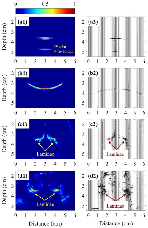
The ultrasonographs (Left) and the corresponding RF data (Right) of the following target: (a) acrylic phantom with the SFS, (b) acrylic phantom with the RCIS, (c) lumbar vertebra phantom, and (d) lumbar vertebra of a subject.
In vivo Study
The decay in echo-amplitude due to the attenuation of ultrasound in the soft tissue was compensated using an -value of 1.65 dB/cm at 3.3 MHz. The measured of the 37 AIS patients ranges from 0.03 to 0.16. For example, the recovered from Figure 5(d2) is 0.07. Based on the magnitude of the curves (Cobb angle – CA), the data was divided into two groups, mild ( < CA ≤24°) and moderate (25°≤CA<45°) curves. Figure 6 plots the measured versus CA; the mild curve group is colored with blue and the latter is shaded with red. The average values for the mild and moderate scoliosis regions are 0.11 ± 0.02 (n = 20) and 0.07 ± 0.03 (n = 17), respectively. Independent T-test analysis was performed to compare the measurements of the two groups (alpha of 0.05). The result shows that the measured values between the two groups are significantly different between the two groups (p-value = 0.0001 < 0.05). There was also a trend observed in the moderate curve region with = 0.3. The best fitting line shows the reflection coefficient declines with the increasing CA, that is, with the severity of the scoliosis.
Figure 6.
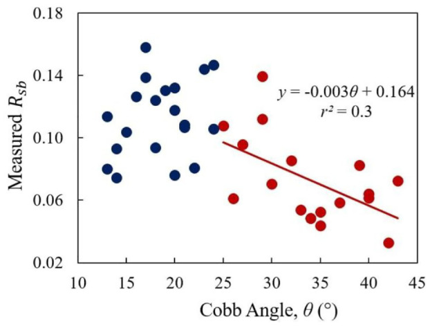
The correlation between the and Cobb angle.
Discussion
The theoretical calculation of the reflection coefficients of the BP and five different materials’ interfaces (acrylic, aluminum, brass, copper, and steel) was matched to the measured values with maximum discrepancy of 6.7% (Table 2). As the stiffness of cortical bone lies between the stiffness values of acrylic and aluminum, it is expected that the reflection coefficient of BP-cortical bone interface is between 0.38 and 0.84.
The surface roughness accounted for approximately 25% of the signal loss while the total effect due to the surface roughness and inclination together caused about 64% loss. When the surface was smoothened, the received signal was back to nearly 90% of the original. The small curve on the surface (SCS) had a small effect on signal loss when compared to the flat surface (SFS). Furthermore, the effect of the tilt angle is actually more significant. Together with the surface roughness, a 3° tilt demonstrated about 40% signal loss while a 5° tilt demonstrated a nearly 70% loss. These experiments demonstrated that a significant amount of energy loss was expected due to both the inclination and roughness of the surface.
From the cadaveric vertebra study, the recovered coefficient is 0.23 ± 0.06, only 33% of the predicted (0.62). Besides, these factors affect the signal loss, the thickness of the human soft tissue may also have effects. Figure 4(c) shows the simulated responses of the amplitude ratio with soft-tissue thickness for three values of . With a constant source amplitude and a fixed tissue thickness, the amplitude of the echo decreases with increasing -value while for a fixed , the amplitude decreases exponentially with thickness. The attenuation coefficient of soft tissue, , in human ranges from 0.3 to 0.8 dB/cm at 1 MHz with an average of about 0.50 dB/cm.37,49 Since the relationship between and frequency is linear,38,50 was extrapolated to be 1.65 dB/cm at 3.3 MHz, which is similar to obtained by the best fitting regression and transmission-through experiments. Ultrasound energy decreases with distance exponentially as it propagates through the absorptive soft tissue. The absorption mechanism dissipates energy within the tissue as heat, reducing the energy and magnitude of the signal. Using the ultrasound images of the 37 AIS subjects, the thickness of soft tissue, measured from the lamina to the skin surface, ranged from 2 to 6 cm with an average of about 3.5 cm. At 3.5 cm soft tissue thickness, the simulated echo-amplitude is only 26% of the source amplitude for = 1.65 dB/cm. Therefore, the effect of soft tissue on the echo-amplitude cannot be ignored.
The effect of absorption upon the reflection coefficient was also studied. The first-order approximation of the amplitude acoustic reflection coefficient for two lossy biological tissues is given by 51
| (7) |
| (8) |
where , is the lossless acoustic reflection coefficient, and is the change of (absorption coefficient per wavenumber) across the tissue interface. Assuming cortical bone has an attenuation coefficient of 45 dB/cm at 3.3 MHz, 52 the absorption term (imaginary component) accounts for less than 10% or precisely 6.8% of the . For the simplicity, we ignore the attenuation effect on the reflection coefficient and only consider the lossless reflection coefficient in this study.
After an approximate compensation of the attenuation in the soft tissue, the measured was in range of 0.03–0.16, lower than the expected values of 0.49–0.64 due to the mentioned loss factors. It is challenging to quantify this loss discrepancy for better estimated Rsb. However, by assuming the loss is similar in each AIS subject, meaningful conclusion could be drawn from the measured . The average value for the moderate curve was lower than that of the mild curve region (0.07 vs 0.11). There was also a mild tendency of decreasing when the curve was larger. A moderate correlation between the and CA was found with of 0.3. Beside this study, Zheng et al. used the reflection index measured in frequency domain to assess bone quality.27,53 This reflection index was found to well correlate with the reflection coefficient with of 0.8. 53 However, their study did not consider the effect of soft tissue thickness variation and the surface roughness. In the earlier studies, Hung et al. and Yip et al. used BMD values to predict the risk of curve progression of scoliosis.20,21 They both found children with scoliosis had lower BMD, but their results did not draw a strong correlation. Furthermore, Zhang et al. utilized bone turnover rate as an index of bone quality to correlate the risk of curve progression. 22 Currently, a randomized control trial is being conducted to investigate if taking more vitamin D supplement can reduce the risk of scoliosis progression. 54 Therefore, understanding the bone health information such as BMD and bone quality can assist orthopedic surgeons to decide treatment planning in a timely manner.
Conclusion
This preliminary study has demonstrated the feasibility of using ultrasonic reflection coefficients for the estimation of material properties and its application in estimating bone properties of AIS patient groups. The total loss in echo amplitude due to the absorptive soft tissue layer, surface roughness and inclination is significant and difficult to quantify. However, although these losses hindered the recovery of true bone properties, the average on the mild curve region was larger than that of the moderate curve region. An inverse relationship between the and CA was found in the AIS group with moderate curves, indicating that bone properties may decrease with the severity of scoliosis. Future investigation of the change of on individual person should be performed to track the risk of progression.
Footnotes
Declaration of conflicting interests: The author(s) declared no potential conflicts of interest with respect to the research, authorship, and/or publication of this article.
Funding: The author(s) disclosed receipt of the following financial support for the research, authorship, and/or publication of this article: The research was supported by the Natural Sciences and Engineering Research Council of Canada and the Scoliosis Research Society.
ORCID iD: Edmond Lou  https://orcid.org/0000-0002-7531-8377
References
- 1. Farady JA. Current principles in the nonoperative management of structural adolescent idiopathic scoliosis. Phys Ther 1983; 63(4): 512–523. [DOI] [PubMed] [Google Scholar]
- 2. Weinstein SL, Dolan LA, Cheng JC, et al. Adolescent idiopathic scoliosis. Lancet 2008; 371(9623): 1527–1537. [DOI] [PubMed] [Google Scholar]
- 3. Cheng JC, Castelein RM, Chu WC, et al. Adolescent idiopathic scoliosis. Nat Rev Dis Primers 2015; 1(1): 15030–15121. [DOI] [PubMed] [Google Scholar]
- 4. Machida M, Weinstein SL, Dubousset J. (eds). Pathogenesis of idiopathic scoliosis. Tokyo: Springer, 2018, pp.27. [Google Scholar]
- 5. Diarbakerli E, Grauers A, Danielsson A, et al. Quality of life in males and females with idiopathic scoliosis. Spine 2019; 44(6): 404–410. [DOI] [PubMed] [Google Scholar]
- 6. Chamberlain CC, Huda W, Hojnowski LS, et al. Radiation doses to patients undergoing scoliosis radiography. Br J Radiol 2000; 73(872): 847–853. [DOI] [PubMed] [Google Scholar]
- 7. Mogaadi M, Ben Omrane L, Hammou A. Effective dose for scoliosis patients undergoing full spine radiography. Radiat Prot Dosimetry 2012; 149(3): 297–303. [DOI] [PubMed] [Google Scholar]
- 8. Nash CL, Gregg EC, Brown RH, et al. Risks of exposure to X-rays in patients undergoing long-term treatment for scoliosis. J Bone Joint Surg. Am 1979; 61(3): 371–374. [PubMed] [Google Scholar]
- 9. Levy AR, Goldberg MS, Mayo NE, et al. Reducing the lifetime risk of cancer from spinal radiographs among people with adolescent idiopathic scoliosis. Spine 1996; 21(13): 1540–1547; discussion 1548. [DOI] [PubMed] [Google Scholar]
- 10. Cook SD, Harding AF, Morgan EL, et al. Trabecular bone mineral density in idiopathic scoliosis. J Pediatr Orthop 1987; 7(2): 168–174. [DOI] [PubMed] [Google Scholar]
- 11. Cheng JC, Qin L, Cheung CS, et al. Generalized low areal and volumetric bone mineral density in adolescent idiopathic scoliosis. J Bone Miner Res 2000; 15(8): 1587–1595. [DOI] [PubMed] [Google Scholar]
- 12. Lee WT, Cheung CS, Tse YK, et al. Association of osteopenia with curve severity in adolescent idiopathic scoliosis: a study of 919 girls. Osteoporos Int 2005; 16(12): 1924–1932. [DOI] [PubMed] [Google Scholar]
- 13. Li XF, Li H, Liu ZD, et al. Low bone mineral status in adolescent idiopathic scoliosis. Eur Spine J 2008; 17(11): 1431–1440. [DOI] [PMC free article] [PubMed] [Google Scholar]
- 14. Lam TP, Hung VW, Yeung HY, et al. Abnormal bone quality in adolescent idiopathic scoliosis: a case-control study on 635 subjects and 269 normal controls with bone densitometry and quantitative ultrasound. Spine 2011; 36(15): 1211–1217. [DOI] [PubMed] [Google Scholar]
- 15. Klibanski A, Adams-Campbell C, Bassford T, et al. Osteoporosis prevention, diagnosis, and therapy. JAMA 2001; 285(6): 785–795. [DOI] [PubMed] [Google Scholar]
- 16. Yu WS, Chan KY, Kwp YU, et al. Bone structural and mechanical indices in adolescent idiopathic scoliosis evaluated by high-resolution peripheral quantitative computed tomography (HR-pQCT). Bone 2014; 61: 109–115. [DOI] [PubMed] [Google Scholar]
- 17. Cheung CS, Lee WT, Tse YK, et al. Generalized osteopenia in adolescent idiopathic scoliosis—association with abnormal pubertal growth, bone turnover, and calcium intake? Spine 2006; 31(3): 330–338. [DOI] [PubMed] [Google Scholar]
- 18. Suh KT, Lee SS, Hwang SH, et al. Elevated soluble receptor activator of nuclear factor-kappaB ligand and reduced bone mineral density in patients with adolescent idiopathic scoliosis. Eur Spine J 2007; 16(10): 1563–1569. [DOI] [PMC free article] [PubMed] [Google Scholar]
- 19. Ishida K, Aota Y, Mitsugi N, et al. Retraction note: Relationship between bone density and bone metabolism in adolescent idiopathic scoliosis. Scoliosis 2015; 10(19): 34. [DOI] [PMC free article] [PubMed] [Google Scholar]
- 20. Hung VW, Qin L, Cheung CS, et al. Osteopenia: a new prognostic factor of curve progression in adolescent idiopathic scoliosis. JBJS 2005; 87(12): 2709–2016. [DOI] [PubMed] [Google Scholar]
- 21. Yip BHK, Yu FWP, Wang Z, et al. Prognostic value of bone mineral density on curve progression: a longitudinal cohort study of 513 girls with adolescent idiopathic scoliosis. Sci Rep 2016; 6(1): 39220–39227. [DOI] [PMC free article] [PubMed] [Google Scholar]
- 22. Zhang J, Cheuk KY, Xu L, et al. A validated composite model to predict risk of curve progression in adolescent idiopathic scoliosis. EClinicalMedicine 2020; 18: 100236. [DOI] [PMC free article] [PubMed] [Google Scholar]
- 23. Lam TP, Hung VWY, Yeung HY, et al. Quantitative ultrasound for predicting curve progression in adolescent idiopathic scoliosis: a prospective cohort study of 294 cases followed-up beyond skeletal maturity. Ultrasound Med Biol 2013; 39(3): 381–387. [DOI] [PubMed] [Google Scholar]
- 24. Du Q, Zhou X, Li JA, et al. Quantitative ultrasound measurements of bone quality in female adolescents with idiopathic scoliosis compared to normal controls. J Manip Physiol Ther 2015; 38(6): 434–441. [DOI] [PubMed] [Google Scholar]
- 25. Chen W, Le LH, Lou EHM. Ultrasound imaging of spinal vertebrae to study scoliosis. Open J Acoust 2012; 2(3): 95–103. [Google Scholar]
- 26. Li H, Le LH, Sacchi MD, et al. Ultrasound imaging of long bone fractures and healing with the split-step Fourier imaging method. Ultrasound Med Biol 2013; 39(8): 1482–1490. [DOI] [PubMed] [Google Scholar]
- 27. Zheng R, Le LH, Hill D, et al. Estimation of bone quality on scoliotic subjects using ultrasound reflection imaging method-a preliminary study. In: 2015 IEEE International Ultrasonics Symposium (IUS), 2015, pp.1–4. New York: IEEE. [Google Scholar]
- 28. Schaffler MB, Burr DB. Stiffness of compact bone: effects of porosity and density. J Biomech 1988; 21(1): 13–16. [DOI] [PubMed] [Google Scholar]
- 29. Helgason B, Perilli E, Schileo E, et al. Mathematical relationships between bone density and mechanical properties: a literature review. Clin Biomech 2008; 23(2): 135–146. [DOI] [PubMed] [Google Scholar]
- 30. Eneh CT, Malo MK, Karjalainen JP, et al. Effect of porosity, tissue density, and mechanical properties on radial sound speed in human cortical bone. Med Phys 2016; 43(5): 2030–2039. [DOI] [PubMed] [Google Scholar]
- 31. Wall JC, Chatterji SK, Jeffery JW. Age-related changes in the density and tensile strength of human femoral cortical bone. Calcif Tissue Int 1979; 27(2): 105–108. [DOI] [PubMed] [Google Scholar]
- 32. Gibson LJ, Ashby MF. Cellular solids: structure and properties. Cambridge: Cambridge University Press, 1999. [Google Scholar]
- 33. Abendschein W, Hyatt GW. 33 ultrasonics and selected physical properties of bone. Clin Orthop Relat Res 1970; 69: 294–301. [PubMed] [Google Scholar]
- 34. Craven JD, Costantini MA, Greenfield MA, et al. Measurement of the velocity of ultrasound in human cortical bone and its potential clinical importance: an in vivo preliminary study. Investig Radiol 1973; 8(2): 72–77. [DOI] [PubMed] [Google Scholar]
- 35. Callens D, Bruneel C, Assaad J. Matching ultrasonic transducer using two matching layers where one of them is glue. NDT E Int 2004; 37(8): 591–596. [Google Scholar]
- 36. Ji Q, Le LH, Filipow LJ, et al. Ultrasonic wave propagation in water-saturated aluminum foams. Ultrasonics 1998; 36(6): 759–765. [Google Scholar]
- 37. Bushberg JT, Boone JM. The essential physics of medical imaging. Philadelphia: Lippincott Williams & Wilkins, 2011. [Google Scholar]
- 38. Hendee WR, Ritenour ER. Medical imaging physics. New York: John Wiley & Sons, 2003. [Google Scholar]
- 39. André MP, Craven JD, Greenfield MA, et al. Measurement of the velocity of ultrasound in the human femur in vivo. Med Phys 1980; 7(4): 324–330. [DOI] [PubMed] [Google Scholar]
- 40. Lees S, Ahern JM, Leonard M. Parameters influencing the sonic velocity in compact calcified tissues of various species. J Acoust Soc Am 1983; 74(1): 28–33. [DOI] [PubMed] [Google Scholar]
- 41. Le LH, Gu YJ, Li Y, et al. Probing long bones with ultrasonic body waves. Appl Phys Lett 2010; 96(11): 114102. [Google Scholar]
- 42. Nazarchuk Z, Skalskyi V, Serhiyenko O. Acoustic emission: methodology and application. Cham: Springer, 2017. [Google Scholar]
- 43. Krautkramer J, Krautkramer H. Ultrasonic testing of materials. 4th ed. Berlin: Springer Science & Business Media, 2013. [Google Scholar]
- 44. Persson HW, Hertz CH. Acoustic impedance matching of medical ultrasound transducers. Ultrasonics 1985; 23(2): 83–89. [DOI] [PubMed] [Google Scholar]
- 45. Rhee S, Ritter TA, Shung KK, et al. Materials for acoustic matching in ultrasound transducers. In: 2001 IEEE ultrasonics symposium proceedings. An international symposium (Cat. No. 01CH37263), 2001, Vol. 2, pp. 1051–1055. [Google Scholar]
- 46. Khodaei M, Hill D, Zheng R, et al. Intra- and inter-rater reliability of spinal flexibility measurements using ultrasonic (US) images for non-surgical candidates with adolescent idiopathic scoliosis: a pilot study. Eur Spine J 2018; 27(9): 2156–2164. [DOI] [PubMed] [Google Scholar]
- 47. Le LH. An investigation of pulse-timing techniques for broadband ultrasonic velocity determination in cancellous bone: a simulation study. Phys Med Biol 1998; 43(8): 2295–2308. [DOI] [PubMed] [Google Scholar]
- 48. Zhang C, Le LH, Zheng R, et al. Measurements of ultrasonic phase velocities and attenuation of slow waves in cellular aluminum foams as cancellous bone-mimicking phantoms. J Acoust Soc Am 2011; 129(5): 3317–3326. [DOI] [PubMed] [Google Scholar]
- 49. Mast TD. Empirical relationships between acoustic parameters in human soft tissues. Acoust Res Lett Online 2000; 1(2): 37–42. [Google Scholar]
- 50. Carstensen EL. The mechanism of the absorption of ultrasound in biological materials. IRE Trans Med Electron 1960; ME-7(3): 158–162. [DOI] [PubMed] [Google Scholar]
- 51. Le LH, Filipow LJ. Approximating the acoustic reflection coefficient of lossy biological tissues. Phys Med Biol 1997; 42(4): 757–758. [DOI] [PubMed] [Google Scholar]
- 52. Lakes R, Yoon HS, Katz JL. Ultrasonic wave propagation and attenuation in wet bone. J Biomed Eng 1986; 8(2): 143–148. [DOI] [PubMed] [Google Scholar]
- 53. Song S, Chen H, Li C, et al. Assessing bone quality of the spine in children with scoliosis using the ultrasound reflection frequency amplitude index method: a preliminary study. Ultrasound Med Biol 2022; 48(5): 808–819. [DOI] [PubMed] [Google Scholar]
- 54. Lam TP, Yip BHK, Man GCW, et al. Effective therapeutic control of curve progression using calcium and vitamin D supplementation for adolescent idiopathic scoliosis – a randomized double-blinded placebo-controlled trial. In: 8th ICCBH, Wurzburg, Germany, 10-13 June 2017, p.34. Bone Abstracts. [Google Scholar]