Metamodeling for Policy Simulations with Multivariate Outcomes

Abstract

Purpose:

Metamodels are simplified approximations of more complex models that can be used as surrogates for the original models. Challenges in using metamodels for policy analysis arise when there are multiple correlated outputs of interest. We develop a framework for metamodeling with policy simulations to accommodate multivariate outcomes.

Methods:

We combine two algorithm adaptation methods – multi-target stacking and regression chain with maximum correlation – with different base learners including linear regression (LR), elastic net (EE) with second-order terms, Gaussian process regression (GPR), random forests (RFs), and neural networks. We optimize integrated models using variable selection and hyperparameter tuning. We compare accuracy, efficiency, and interpretability of different approaches. As an example application, we develop metamodels to emulate a microsimulation model of testing and treatment strategies for hepatitis C in correctional settings.

Results:

Output variables from the simulation model were correlated (average ρ=0.58). Without multioutput algorithm adaptation methods, in-sample fit (measured by R²) ranged from 0.881 for LR to 0.987 for GPR. The multioutput algorithm adaptation method increased R² by an average 0.002 across base learners. Variable selection and hyperparameter tuning increased R² by 0.009. Simpler models such as LR, EE, and RF required minimal training and prediction time. LR and EE had advantages in model interpretability, and we considered methods for improving interpretability of other models.

Conclusions:

In our example application, the choice of base learner had the largest impact on R²; multioutput algorithm adaptation and variable selection and hyperparameter tuning had modest impact. While advantages and disadvantages of specific learning algorithms may vary across different modeling applications, our framework for metamodeling in policy analyses with multivariate outcomes has broad applicability to decision analysis in health and medicine.

INTRODUCTION

Simulation modeling is commonly used in health policy analyses, including cost-effectiveness analyses (CEA). Increasingly complex simulation-based CEA models have been developed as computational power and data availability have increased. Greater model complexity often translates into longer computation times. For example, many runs may be needed to reduce the Monte Carlo error in a complex stochastic simulation model or to perform sensitivity analyses that provide insights from models with large numbers of parameters. At the same time, stakeholders often want model-based tools to support decision making in their local environments, which might not be readily available or easily translated from a policy model published in a peer-reviewed article. Local contextualization of modeling studies may be facilitated by web-based applications that accommodate more flexible real-time model adaptations. Key factors for the successful deployment of such a tool are a user-friendly interface and fast model run-time, as well as the suitability and validity of the model to answer the question at hand.¹ Model interpretability is also critical so that stakeholders can understand a model’s inputs and assumptions, identify relationships between model inputs and outputs, and avoid the perception of the model as a ‘black-box.’^2–4

The Second Panel on Cost-effectiveness in Health and Medicine stressed the importance of efficient model emulators, or metamodels, as a means of reducing computational cost.⁵ A metamodel is a statistical approximation of an originally constructed model. In addition to serving as a proxy model that can replace a more complex model to predict outputs, metamodels can also be used to improve interpretability⁶ and aid in model calibration.⁷ For example, linear regression, which can serve as a metamodel for the original simulation model if prediction accuracy is satisfactory, can improve the interpretability of the original model by identifying a clear (albeit approximate) relationship between model inputs and outputs.¹ Computational requirements for such a metamodel are small, thereby facilitating tasks such as model calibration and probabilistic sensitivity analysis and increasing the potential for use of the metamodel in a web-based modeling tool.

Metamodels have a long history of use as surrogates for more complex original models, within a range of areas including public health, energy and the environment, and queueing systems.^8–10 In health policy research, use of metamodels has been driven by the need to reduce computational complexity, facilitate value-of-information analysis, and help reduce decision uncertainty given model input uncertainty.^11–18 To build a good approximation of an original model, various methods, such as linear regression, logistic regression, Gaussian process regression, and artificial neural networks have been used.^{11, 13, 14, 19–21} Degeling et al. recently provided a step-by-step guide to developing metamodels in the health economics research setting.²²

A limitation of existing methods for metamodeling is that such methods typically do not consider the challenges that arise when multiple output variables are relevant to a particular policy analysis, and when those outputs are correlated (e.g., the costs and health effects of different policy choices).^{1, 21, 23} When outputs are correlated, an approach that does not account explicitly for these correlations could lead to invalid conclusions, for example when comparisons between the outcomes are salient (as in the ranking of alternatives on a particular measure) or when the key quantity of interest depends on multiple outcomes.

In this paper, we develop a framework for metamodeling of simulation models that accommodates multiple correlated outcomes, and we compare alternatives for the choice of base learning algorithm. As an example, we apply our framework to develop a metamodel based on a microsimulation model of alternative testing and treatment strategies for hepatitis C in correctional settings. We show how metamodeling can provide accurate predictions of outputs and improve computational efficiency and model interpretability.

METHODS

In this section, we introduce a general framework for constructing metamodels, present details of our method for handling multioutput prediction, describe different base models that can be used to emulate the original model, and describe our model-independent variable selection scheme. We also present evaluation metrics for the constructed metamodels.

Metamodeling Framework

Creation of a metamodel involves development of standardized input and output variable sets, splitting the data into training and testing sets, and then finding the best model to approximate the relationships between the inputs and outputs.²²

A first step is to generate appropriate data for constructing the metamodels, which comprise inputs and outputs from a full ‘original’ model that will be emulated by the metamodel. We start with N sets of values for the array of input variables used in the original model. If all input variables are independent, random samples can be drawn from the distribution of each input variable and integrated into the N sets of values. Otherwise, the joint distribution of all input variables must be sampled to generate these sets of input values. Depending on the modeler’s knowledge of the study population and context, other more efficient sampling methods such as stratified sampling and cluster sampling can be used. Many modelers use a Bayesian approach to obtain input variable sets via model calibration, a process that yields a joint distribution of values for all parameters that reflects their correlation structure.²⁴ The necessary number of input variable sets N depends on the complexity of the model as reflected by factors such as the number of input variables, the number of outputs of interest, and the dynamics of the processes being simulated. For each set of values of the input variables, the original model is simulated to generate a corresponding set of output values. Via metamodeling we then aim to build a simplified version of the original model that can approximately replicate the same relationships between inputs and outputs produced by the original model.

Depending on the data, preprocessing may be necessary before a model can be built. If the data include categorical variables, they must be converted, either to multiple one-hot vectors (these are vectors where all elements except one are set to zero) or to an ordinal variable, depending on the relationships between different categories. Such transformation is necessary since many machine learning models do not inherently handle categorical variables.

After appropriate transformation of categorical variables to one-hot vectors, input and output variables may be standardized.²⁵ This is done using the formula $z_i^{\left(j\right)}=\frac{x_i^{\left(j\right)}-\overline{x_i}}{s_i}$ where $x_i^j$ is the j-th x_i value in the array of n input variables, and ${\overline{x}}_i$ and s_i are the sample mean and standard deviation, respectively. We perform a similar standardization on the output variables. There are many reasons for performing such scaling, including improving the training process of models such as neural network models via stochastic gradient descent and improving model stability.²⁶ Another important reason for scaling is due to the multioutput structure. Standardization also allows combination of loss functions that may have different scales. A disadvantage of standardization is that it can complicate interpretation of the relationships between input and output variables.

The final step before building the metamodel is to randomly split the data into training and testing datasets. The training phase is divided into two steps: a performance improvement phase with hyperparameter tuning and variable selection, and actual training with selected variables and specified model hyperparameters. We present details of the variable selection scheme below. For the actual training phase, 10-fold cross-validation is utilized.²⁷ Under this approach the training dataset is further split into 10 folds, and one at a time each of the 10 folds is withheld while the other 9 folds are used to build the model. Model performance is then evaluated with respect to the withheld data in order to identify the best-performing model based on defined evaluation criteria.

Multioutput Regression

Most simulation models in public health generate multiple outputs of interest (e.g., costs and multiple health outcomes, possibly in different population groups).^{1, 21, 23} Because metamodeling aims to build a replacement model to link the original simulation inputs and outputs, approaches can be generalized from multioutput regression. There are two main approaches: problem transformation and algorithm adaptation.²⁸ In problem transformation, multioutput regression is transformed to separate single-output predictions. Algorithm adaptation methods can be readily integrated with any single-output prediction model to predict all the outputs simultaneously.²⁸ Algorithm adaptation methods such as multi-target stacking (MTS) regression and regression chains have been shown theoretically to perform better than problem transformation methods.²⁸ There are several regression chain variants. Use of a regression chain with maximum correlation (RCMC), has been shown to outperform other methods over a range of different datasets in terms of accuracy and to require less computational power than other methods such as ensemble regression chains.²⁹ We use RCMC and MTS in our study.

We first describe multioutput regression and provide notation that will be used subsequently. X denotes the input matrix which consists of d input variables (X₁, X₂,⋯, X_d). Y denotes the output matrix which consists of m output variables (Y₁, Y₂,⋯, Y_m). We have a training set D = {( x¹, y¹), …, (xⁿ, yⁿ)}, and our target is to learn a model $H:\mathcal{X}\to \mathcal{Y}$ so that h(x) (x is a random input vector) best approximates y (the corresponding output vector).

To build an MTS model, we follow a two-stage approach. In the training phase, we first build m single-output prediction models. Then we stack input variables to m −1 output variables (X₁, X ₂,⋯, X_d, Y₁, ⋯, Y_{k ― 1}, Y_{k + 1}, ⋯, Y_m) to predict Y_k. In the testing phase, we use the first stage single-output prediction models to obtain a predicted Ŷ. We then use the predicted Ŷ together with X to predict the final Ŷ.

To build an RCMC model, we calculate the correlation coefficients between output variables, ρ_ij (where i and j indicate different output variables Y_i and Y_j with 1 ≤ i ≠ j ≤ m) and calculate the average correlation coefficient ${\rho }_i=\frac{{\sum }_{j=1}^m{\rho }_{ij}}{m-1}$ (where i ≠ j) for each variable, averaged across all j covariables. We rank the average correlations in descending order and use the order to determine the sequence of prediction, represented by (Y′₁, Y′₂⋯Y′_m). If there are only two output variables (Y₁ and Y₂), we would randomly order these two outcome variables since ρ₁ and ρ₂ are equal. For the first prediction model, we build a single-output prediction based on the inputs (X₁, X₂,⋯, X_d) and (Y′₁ ). Subsequently, we use inputs (X₁, X₂,⋯, X_d) and the previously used output variables (Y₁′, Y₂′, ⋯, Y′_k ― 1) together to predict the new output variable (Y′_k). One caveat is that Y′₁ will not be available in the prediction task after the model is constructed. Therefore, the prediction model will use previously predicted outputs. In other words, to predict $\left({{\widehat{Y}}^{\text{'}}}_k\right)$, the values (X₁, X₂,⋯, X_d) and $\left({{\widehat{Y}}^{\text{'}}}_1,{{\widehat{Y}}^{\text{'}}}_2,\cdots ,{{\widehat{Y}}^{\text{'}}}_{k-1}\right)$ are used.

Base Learners

The regression chain introduced above adapts to the base learner $h_k^{\text{'}}\text{:}\mathcal{X}\to {Y^{\text{'}}}_k$. A wide range of choices exists for the base learner. After reviewing other metamodels constructed for health economics studies^{1, 30}, we chose the following five widely used methods: linear regression, elastic net with second-order terms, Gaussian process regression, random forest, and neural network. For each method, we record the performance of the method in predicting individual outcomes one at a time $\left(h_k\text{:}\mathcal{X}\to {\mathcal{Y}}_k\right)$ as well as the performance when using RCMC or MTS together with the base learner.

Linear Regression (LR)

Linear regression (LR) is a popular metamodeling method because of its fast implementation and easy interpretability. The performance of LR can be comparable to or even better than more sophisticated statistical models when data are sparse or scarce. For our setting, data sparsity is not a problem since we can use the original model to generate a sufficient number of data points. We use LR as a baseline for performance evaluation.

Elastic Net with Second-Order Terms (EE)

Elastic net is a linear regression that includes penalty terms that help overcome the problem of overfitting and reduce model complexity.²⁵ To increase prediction power, second-order terms are added to the original input space together with the elastic net model (EE) to capture non-linear relationships between inputs and outputs. We choose elastic net regularization to overcome the problem of over-fitting and to allow for flexibility between first-order (Lasso) and second-order (Ridge) regularizations, since the relative performance of Lasso and Ridge will depend on the distribution of true regression coefficients.³¹

Gaussian Process Regression (GPR)

Gaussian process regression (GPR) is a Bayesian non-parametric kernel-based probabilistic model. GPR assumes that the distribution of output data $\left\{f\left(x\right),x\in {ℝ}^d\right\}$ is a joint Gaussian distribution specified by mean function mean(x) and covariance/kernel function kernel(x, x′). In general, similar input data will have similar output values. We use GPR with a Matérn kernel due to its flexibility in allowing for control of smoothness and because it can replicate different kernels by changing model hyperparameters.³²

Random Forest (RF)

Random forest (RF) is an ensemble machine learning method that constructs multiple decision trees and uses maximum voting or averages over all individual trees to obtain the outputs. RF imposes no assumptions on the data and usually produces high prediction accuracy even without hyperparameter tuning.³³

Neural Network (NN)

Neural networks (NN) are a class of machine learning models and algorithms that use connected, hierarchical functions.³⁴ We use multilayer perceptron, a technique that employs backpropagation for training: a feedforward neural network model comprises an input layer, a changeable number of middle layers, and an output layer. Each input/output variable is modeled by a neuron in the NN. Each neuron node value is determined by all connected neurons from the last layer which follows as $f\left(x\right)=\varphi \left(\sum w_i{x}_i\right)$. The activation function ϕ( ∙ ) is a predefined non-linear function to capture the non-linearity in the data.

Performance Improvement Scheme

We consider two ways of improving model performance: model-free variable selection and hyperparameter tuning for different base models. With RCMC, we have one regression model for each output variable but the input variable set is modified since we need to include the previous predicted output variables in the subsequent models. Variable selection works on the newly constructed input variable set, which includes both the original input variables plus the new predicted output variables.

Variable Selection

To improve model performance, as well as interpretability, we implement a variable selection scheme that is model-free and can be integrated into the training process. The objective is to search for the subset of input variables that will result in the best model performance. However, because of limitations on computational power and the typically large number of input features in simulation models in public health, it is not feasible to perform an exhaustive search over all potential subsets of input variables.

We therefore use the following greedy search algorithm (i.e., an algorithm that follows the problem-solving heuristic of making the locally optimal choice at each stage) for variable selection:

• Step 1: Start with the full input variable set.

• Step 2: Remove the least important input variable according to the following steps.

  • Randomly permute each input variable (i.e., randomly arrange the order of the values for the chosen variable).
  • Compute the resulting accuracy reduction from having each permuted input variable rather than the actual values for that variable in the validation dataset.
  • Remove the input variable with the smallest reduction in prediction accuracy.

• Step 3: Compute model performance by calculating the average of coefficient of determination (average R²) for the remaining subset of input variables. Go to Step 2 if the number of variables is more than 1; otherwise, go to step 4.

• Step 4: Select the optimal subset of input variables based on model performance (R² value).

By permuting an input variable, we remove the relationship between that input variable and the outcome variables. If the input variable is important, the accuracy of the model will decrease because of the loss of information from that input variable. In this way, we aim to identify the most important input variables.

Hyperparameter Tuning

A hyperparameter is a parameter whose value is set before the learning process begins (e.g., the number of trees considered in an RF algorithm). In hyperparameter tuning, hyperparameters are varied to determine the best hyperparameters for a learning algorithm. Table 1 shows the hyperparameters for each of the five base models that we examined. Due to limited computational power, we chose a fixed set of hyperparameters based on a review of the literature and experience of modelers.^{10, 35, 36}

Table 1.

Summary of explored hyperparameters (default parameters are bolded)

Model	Explored Hyperparameters
Linear regression	None
Elastic net	1. α = [0.01, 0.1, 1] 2. ρ = [0.1, 0.5, 0.9]
Gaussian process regression	1. Kernel: [Radial Basis Function, Matérn with γ = 1/2,3/2, 5/2]
Random forest	1. # of variables to sample: $\left[lo{g}_{2}D,⌊\sqrt{\mathbf{D}}⌋,\frac{1}{2}D,D\right]$ 2. # of trees: [100, 500, 1000]
Neural network	1. # of hidden layers: [1,2] 2. # of neurons in hidden layer:  1 Layer: [D, 2 D]  2 Layers: [(D,16), (2D, 16), (D,8), (2D,8)] 3. Activation functions: ReLU, tanh, sigmoid

Evaluation Metrics

Model Accuracy

To compare the performance of different models over multiple outcome variables, we calculate the average R².²⁹ This is calculated as:

$$\text{average} R^2={\sum }_{j=1}^{m}1-\frac{{\sum }_{i=1}^n{\left(y_j^{\left(i\right)}-f_j\left(x^{\left(i\right)}\right)\right)}^2}{{\sum }_{i=1}^n{\left(y_j^{\left(i\right)}-{\overline{y}}_j\right)}^2}$$

where $y_j^{\left(i\right)}$ is the i-th data point for the j-th output variable, f_j( ∙ ) is the trained metamodel for the j-th output variable, ${\overline{y}}_j$ is the average over the j-th output variable and x⁽ⁱ⁾ is the i-th input variable. Since we focus on overall average performance across different outcome variables when choosing the metamodels, we do not analyze model performance on individual outcome variables.

Computational Efficiency

In addition to accuracy, we assess computational efficiency, which we characterize by the CPU time required for training and prediction as a function of the number of input variables and the number of data points in the respective dataset. Our model was developed and run on a 2.5GHz quad-core Intel Core i7 processor. For reference, the original analytic model, implemented in C++ and R, took approximately 70 minutes to evaluate a single set of parameter input values. Over 2,000 unique parameter sets, the runtime was an estimated 17 hours when distributed across 150 nodes of a high-performance computing cluster.

Model Interpretability

Model interpretability is frequently an important goal of metamodeling, especially for models used in public health. We consider model interpretability in terms of how well a model accommodates understanding of the relationships between inputs and outputs, which is important for models that aim to inform policy decisions. Some models are intrinsically interpretable, but others are too complex to understand and require post-hoc methods to improve interpretability.

For model interpretability, LR and EE have clear advantages. LR is the most interpretable since regression provides a closed-form solution with calculated coefficients that characterize the relationship between inputs and outputs. However, if the relationship between inputs and outputs is not linear, making linear inferences based on coefficient values could be misleading. EE has slightly less interpretability compared to LR because of the regularization terms (i.e., terms that add penalties for complexity): for instance, no closed-form solutions on standard error estimates are provided. RF is an aggregation of single decision trees. Even though the decision trees are intrinsically interpretable, the ensemble of multiple trees distorts the original simple interpretable structure. GPR is conceptually easy to understand and its probabilistic structure can provide uncertainty bounds around predictions, but the inclusion of different kernels obscures the relationship between outputs and inputs. NN models are the least interpretable due to the addition of multiple layers and different activation functions.

To facilitate model interpretation, we can use different model-agnostic tools, which can be divided into global and local interpretation methods. Global interpretation methods aim to illuminate the relationship between input and output variables. The variable importance calculation determined from the variable selection scheme is a good way to assess the magnitude of the impact of each input variable on the output variables.

To further understand the relationships between input and output variables, we can use a partial dependence plot, which is similar to one-way or two-way sensitivity analysis in health policy analysis. The partial function ${\widehat{f}}_{x_s}$ (where x_s is the input variable of interest) is estimated by calculating over the training data: ${\widehat{f}}_{x_s}=\frac{1}{n}{\sum }_{i=1}^{n}f\left(x_s,x_c^{\left(i\right)}\right)$ where the terms $x_c^{\left(i\right)}$ are all other input variables. Another way to achieve global interpretability is to generate a global surrogate model, which is an interpretable model (like a decision tree or linear regression) that can replicate the prediction of the original analytical model to the greatest extent.³⁷

Local model interpretation provides insights into an individual prediction of any black-box model. Similar to a global surrogate model, a local surrogate model (LIME, or local interpretable model-agnostic explanation) aims to replicate the prediction of the original analytical model at individual data points by weighting permuted samples based on proximity to the data point of interest.

Case Study: Hepatitis C Virus Testing and Treatment

We illustrate our methods with an individual-based microsimulation model that assesses the clinical outcomes, cost-effectiveness, and budgetary impact of various hepatitis C virus (HCV) testing and treatment strategies in US prisons.³⁸ Our goal was to develop a simplified model that can be used as a tool by local and regional planners to develop HCV testing and treatment strategies by correctional facilities in their jurisdictions.

For the metamodeling analysis, we considered five outcomes: 1) the number of HCV cases identified (by risk-based testing or testing all individuals, depending on the strategy), 2) the number of HCV cases cured, 3) testing cost, 4) treatment cost, and 5) total cost. The original microsimulation analysis considered 15 different HCV testing and treatment strategies, in addition to the status quo of no testing and no treatment. After discussions with stakeholders, we narrowed our focus to six strategies to evaluate using metamodeling, all compared to the status quo: risk-based testing, treating only individuals whose HCV infection has progressed to fibrosis stage F3 or higher (F3+); risk-based testing, treating only individuals whose HCV infection has progressed to fibrosis stage F2 or higher (F2+); risk-based testing, treating all patients with HCV (treat all); test all, treat F3+; test all, treat F2+; test all, treat all. We considered two different time horizons (1 year and 2 years). This yielded a total of 60 output variables (five outcomes for six strategies over two time horizons).

To determine which of the 50 simulation input variables to use, we first ran the simulation model to determine the relative importance of the different variables. We used this information to shorten the list of input variables. We consulted with stakeholders to understand how likely it was that they could provide estimates for each of the remaining input variables. We thereby selected 37 of 50 input variables from the simulation model that stakeholders and the modelers who developed the simulation model deemed the most important. Preliminary analyses indicated that some of these 37 variables had no impact on the 60 output variables, so we further shortened the list to 22 input variables (Supplemental Table S1).

We created datasets using a random design. We drew 2,000 independent samples from each of the specified distributions for the 22 input variables, holding all other parameters fixed at their mean values, and fed these 2,000 input variable sets into the original simulation model. To minimize Monte Carlo noise, we ran the simulation model with 1,000,000 individuals for each input variable set. We randomly divided the 2,000 sets of input and output variables into a training set with 1,600 sets and a test set with 400 sets. The 10-fold cross validation procedure described above was used within the training dataset, and the final performance of the model selected through that procedure was evaluated using the test set.

We implemented five single-prediction models corresponding to five base learners: LR, EE, GPR, RF, and NN. We then implemented MTS and RCMC for each base learner. The final two sets of models focused on improving the performance of MTS and RCMC models with variable selection and hyperparameter tuning.

RESULTS

The output variables from the simulation model were correlated (average ρ=0.58), suggesting a potential need for our methods.

Model Accuracy

Table 2 shows the average coefficient of determination (average R²) for each model considered. Looking at the single-output case – that is, without multioutput algorithm adaptation methods – the worst-performing model was simple linear regression, with an R² of 0.881. Next best were EE and RF, which both had an R² of 0.954 for the single-output case, followed by NN with an R² of 0.965, and GPR with an R² of 0.987. The single output GPR model outperformed all other models except for NN with MTS and variable selection. Although this observation might be limited to this case study, GPR has been shown in many metamodeling studies to provide highly accurate predictions that are robust to changes in data.^{10, 14, 16, 19}

Table 2.

Summary of model performance (average R²) on test dataset for hepatitis C virus model

Model	LR	EE	GPR	RF	NN
Single Output	0.8812	0.9536	0.9865	0.9536	0.9651
RCMC	0.8814	0.9539	0.9875	0.9552	0.9672
RCMC + VS	0.8822	0.9571	0.9917	0.9598	0.9809
RCMC + VS + HT	-	0.9598	0.9921	0.9605	0.9833
MTS	0.8815	0.9541	0.9874	0.9556	0.9679
MTS + VS	0.8824	0.9564	0.9917	0.9584	0.9871
MTS + VS + HT	-	0.9592	0.9919	0.9608	0.9829

LR = linear regression, EE = elastic net, GPR = Gaussian process regression, RF = random forest, NN = neural network, RCMC = regression chain with maximum correlation, VS = variable selection, HT = hyperparameter tuning (LR does not have HT), MTS = multi-target stacking

Inclusion of the multioutput algorithm adaptation methods increased R² for all models, as expected, although the improvements were small. RCMC and MTS increased R² by 0.002 on average across all base learners, and variable selection and hyperparameter tuning added 0.009 on average. The best performing model, GPR, had an R² of 0.992 with RCMC, variable selection, and hyperparameter tuning – an extremely high level of accuracy.

Although we measured accuracy using average R² across all five output variables, we note that there were some differences in performance with respect to different outcomes. For example, the prediction of number of HCV cases identified had a higher R² value than the prediction of total costs.

Computational Efficiency

Figure 1 summarizes key results relating to computational efficiency for each model. Figures 1a and 1b show the relationships between training time and the number of variables and the size of training dataset. For a dataset of size 1600, training the neural network was the most time-consuming task, requiring a maximum of 58.6 seconds to train one output variable when the number of input variables equaled 80, whereas linear regression only took 0.009 seconds to train one output variable (Figure 1a). NN is time-consuming to train. Its run time is positively correlated with the number of input variables and the size of the training dataset because of an increase in the number of edges from input neurons to hidden layers (in our model, the number of hidden neurons was also positively correlated with the number of input variables) and the number of data points to be used in the training. With 22 input variables, training GPR was the most time-consuming task, requiring a maximum of 15 seconds to train on a dataset of size 1600, whereas LR only required 0.002 seconds (Figure 1b). The training time for GPR is greatly affected by the number of input data points because of the difficult operations on large kernel matrices used to handle large training data size. The training time of RF was lower than that of NN and GPR. EE and LR had the lowest average training times. Because we might need to use hundreds or even thousands of training runs to cover different output variables and employ different performance improvement schemes, the total amount of time spent in the training phase can be very lengthy for GPR and NN.

Figure 1/.

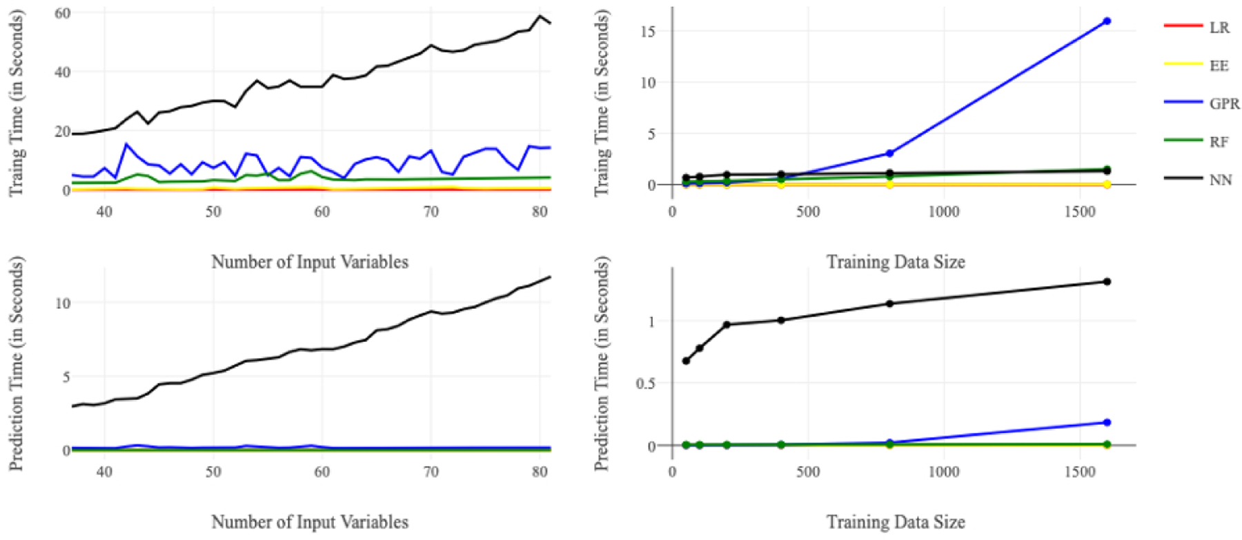
Average training and prediction times for the five base models Top Left (a): Average training time for each model versus number of input variables (D) when training data size (N_train) = 1600; Top Right (b): Average training time for each model versus training data size (N_train) when number of input variables (D) = 22; Bottom Left (c): Average prediction time for each model versus number of input variables (D) when testing data size (N_test) = 400; Bottom Right (d): Average prediction time for each model versus training data size when number of input variable (D) = 22 and testing data size (N_test) = 400

LR = linear regression, EE = elastic net, GPR = Gaussian process regression, RF = random forest, NN = neural network

Figures 1c and 1d show the relationships between prediction run times and the number of variables and the size of the training dataset for a testing dataset of size 400. For the prediction task, NN required the most time of the five methods we tested. With 80 input variables, NN took a maximum of 11.4 seconds to finish the prediction task, whereas LR only took 0.0002 seconds (Figure 1c). With 22 input variables, NN required a maximum of 1.3 seconds for prediction whereas LR required 10⁻⁷ seconds (Figure 1d). The prediction time of NN increases with the number of input variables due to the increased neural net complexity and with the size of the training set. The other four models have a very short prediction time for the testing dataset size of 400. In all cases, the prediction time was on the order of seconds. This is in contrast to the original microsimulation model where a single run took approximately 70 minutes of computation time.

Model Interpretability

To facilitate model interpretation, we examined variable importance, as calculated in the variable selection process (using the greedy search algorithm), for predicting the number of HCV cases identified by risk-based testing in one year. After the selection process, 3 variables were retained in RF and 11 variables were retained in GPR. For both RF and GPR, the most important variable in determining the number of HCV cases identified was the percentage of current injection drug users (IDUs) in the population (Table 3). This is not surprising since risk-based testing strategies defined eligibility for testing using IDU status. The second influential variable was the prevalence of chronic HCV infection in prison. All other variables had far less importance.

Table 3. Variable importance results from RF (random forest) and GPR (Gaussian process regression) for predicting the number of hepatitis C virus (HCV) cases identified in one year by risk-based testing.

Weights are defined as mean decrease in R². Variable definitions are as follows: idu_status_current = % of people who are current drug injectors; idu_status_none = % of people who are not drug injectors; idu_status_former = % of people who are former drug injectors; chronic_hcv_v2 = % of people with chronic HCV infection; sex_male_prev_v2 = % males in the cohort; age_mon_miu = mean age in months; age_mon_sd = standard deviation of age in months; sentence_dur_mon_miu = mean sentence

A. Variable importance for RF
Variable	Weight (mean ± std)
idu_status_current	0.8846 ± 0.0774
chronic_hcv_v2	0.2392 ± 0.0121
age_mon_miu	0.0205 ± 0.0015
B. Variable importance for GPR
Variable	Weight (mean ± std)
idu_status_current	0.8592 ± 0.0600
chronic_hcv_v2	0.3865 ± 0.0553
idu_status_none	0.0323 ± 0.0007
idu_status_former	0.0303 ± 0.0024
age_mon_miu	0.0156 ± 0.0014
sentence_dur_mon_miu	0.0103 ± 0.0030
sentence_dur_mon_sd	0.0094 ± 0.0015
age_mon_sd	0.0033 ± 0.0005
test_specif	0.0022 ± 0.0007
lab_test	0.0021 ± 0.0003
sex_male_prev_v2	0.0005 ± 0.0001

To further understand the relationship between the input and output variables, we examined the partial dependence plots for IDU prevalence and chronic HCV prevalence. The horizontal axes in Figures 2a and 2b are input variables – prevalence of chronic HCV and IDU prevalence (after standardization in the preprocessing step); the vertical axis is the output variable – the number of HCV cases identified (after standardization) in one year under the risk-based testing strategy. The number of HCV cases identified increases as chronic HCV and IDU prevalence increase, for both RF (Figure 2a) and GPR (Figure 2b). The change in the number of HCV cases identified is more sensitive to changes in IDU prevalence than to changes in chronic HCV prevalence because these examples assume risk-based testing.

Figure 2/.

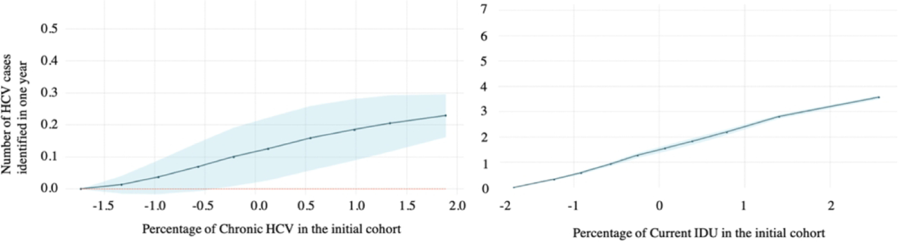
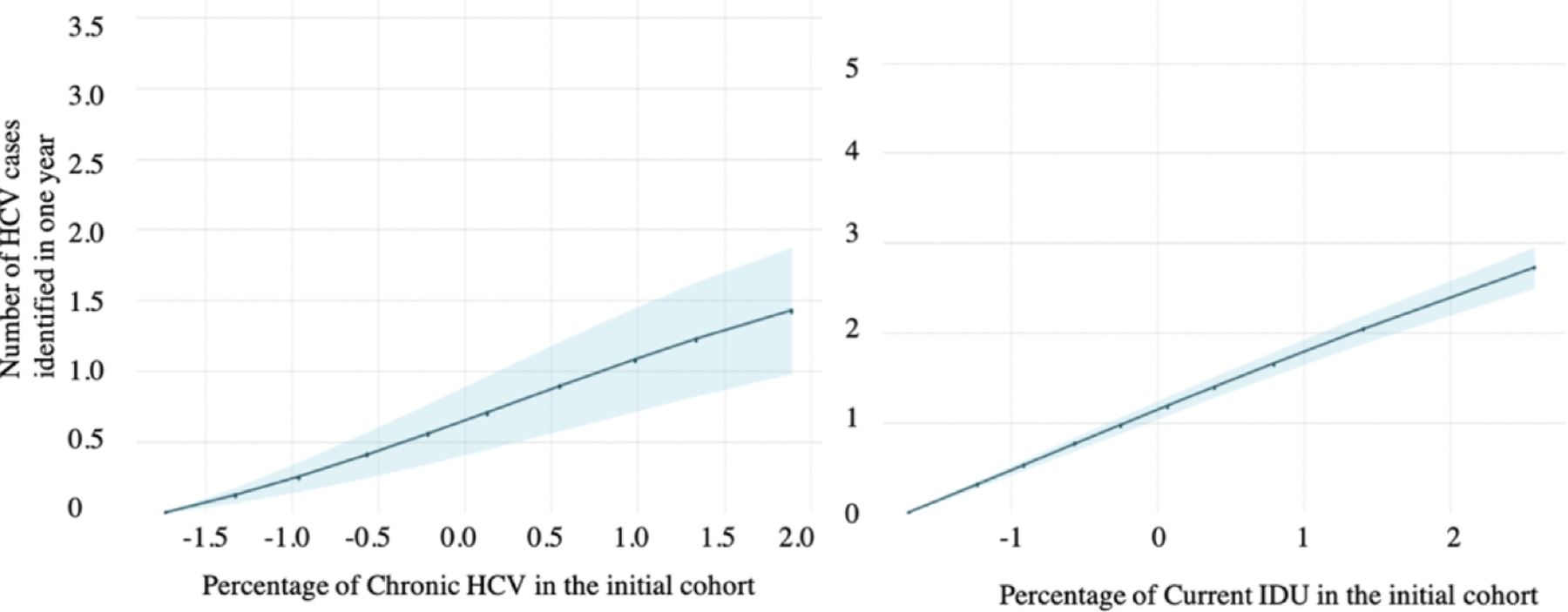
Partial dependence plots from (A) random forest and (B) Gaussian process regression for predicting the number of hepatitis C virus (HCV) cases identified in one year by risk-based testing. Within each row of figures, the first figure shows the partial dependence on the prevalence of chronic HCV in the initial cohort, and the second shows partial dependence on the prevalence of current IDU in the initial cohort. The blue shaded region in each graph is the 95% confidence interval.

A. Partial dependence plots from random forest (RF)

B. Partial dependence plots from Gaussian process regression (GPR)

Figure 3 shows the weight for each variable in the local approximation (or LIME) model to explain one test data point for RF (Figure 3a) and GPR (Figure 3b) in predicting the number of HCV cases identified in one year. The LIME algorithm finds a linear regression model that fits to neighboring points around the point of interest. The coefficients for each input variable are shown on the horizontal axis. The size of the bar indicates the coefficient magnitude and the color of the bar indicates positivity of the coefficient. Figures 3a and 3b both show that each unit increase in IDU prevalence had a larger impact on the output variable than a unit increase in chronic HCV prevalence, with the effect significantly larger for RF. This matches the observations from the partial dependence plots shown in Figure 2.

Figure 3/.

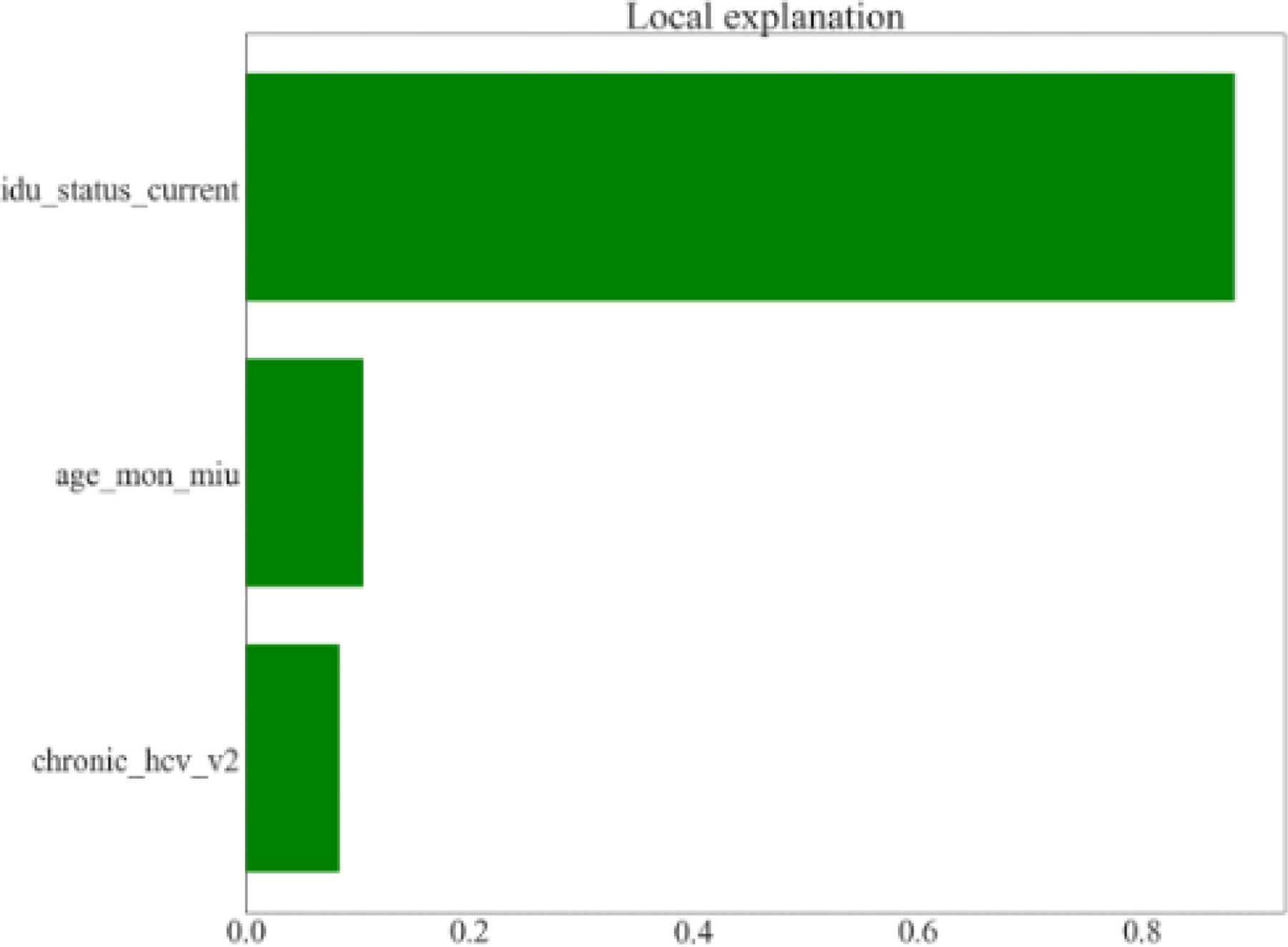
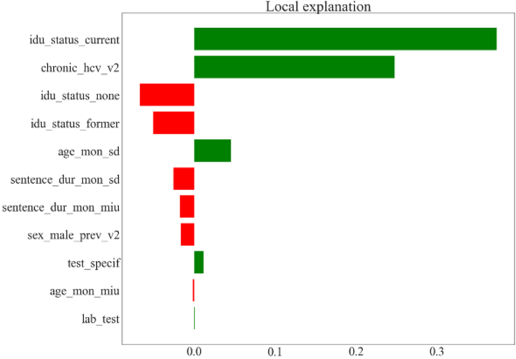
Prediction of the number of hepatitis C virus (HCV) cases identified in one year by risk-based testing. LIME (local interpretable model agnostic) models from RF (random forest) and GPR (Gaussian process regression) for one test data point when limiting the local linear regression variables to variables found by variable selection. The bar width is the weight of each variable in the local regression. The local regression has a bias term. Variable definitions are as follows: age_mon_miu = mean age in months; age_mon_sd = standard deviation of age in months; chronic_hcv_v2 = % of people with chronic HCV infection; idu_status_current = % of people who are current drug injectors; idu_status_former = % of people who are former drug injectors; idu_status_none = % of people who are not drug injectors; lab_test = type of fibrosis staging test (APRI or fibroscan); sentence_dur_mon_miu = mean sentence duration in months; sentence_dur_mon_sd = standard deviation of sentence duration in months; sex_male_prev_v2 = % males in the cohort; test_specif = specificity of fibrosis staging test.

A. LIME model from random forest (RF)

B. LIME model from Gaussian process regression (GPR)

DISCUSSION

Prediction accuracy is one important metric for assessing a metamodel. For some simulation models, including the example used in this paper, there may be a clear relationship between input and output variables that even simple learners like LR can approximate (R² = 0.8812 for our case study). In our analyses, two factors improved prediction accuracy: the choice of base learner and the employment of a multioutput algorithm adaptation method. Moving from LR to GPR increased the prediction accuracy from 0.8812 to 0.9865, indicating the importance of selecting a good base learner. Achieving such an improvement is important in health policy settings since decisions informed by a metamodel can have profound effects on individual health as well as overall population costs and benefits.

Inclusion of the multioutput algorithm adaptation methods MTS and RCMC in our study increased R² by 0.002 on average across the five base learners we considered. One possible reason for the small increase is that our dataset of inputs and outputs, generated from a carefully constructed simulation model, already exhibits strong correlations between certain input and output variables, so the transformation of the input variable set by including output variables does not provide sufficient additional information for improvement. The simplest model (LR) achieved an R² of 0.89, limiting the potential improvement from alternative base learners and performance improvement schemes. In general, we expect that the magnitude of the benefit will vary across different applications, as RCMC and MTS have been shown to significantly improve regression model accuracy in other applications.²⁸

Variable selection and hyperparameter tuning added 0.009 on average to R² in our case study. Variable selection improved model accuracy while also shortening the list of variables that end-users need to consider. Depending on the metamodeling application, there may be additional criteria that are important to consider in determining final variable selection, including face validity, and such criteria may counterbalance our emphasis on parsimonious predictive validity. Hyperparameter tuning can also improve model accuracy, but the results will depend on the number of different hyperparameters searched, potentially requiring very high computational power.

In addition to model accuracy, other factors such as model efficiency and interpretability are also important in our setting. All of the metamodels had very short computation times, much shorter than the computation time required for the original model, and thus any of them could be instantiated as a tool for decision makers. The importance of computation time may depend on the use-case for the metamodel: for example, an interactive model operationalized as a web-based tool may require a different level of real-time responsiveness to changing inputs than a model used for more circumscribed investigations in which interactive functionality may be less central. LR has an advantage in its simplicity, versatility, and interpretability. Another advantage of LR is that it is easy to obtain a prediction interval. This is useful in public health where stakeholders and policy makers often want to know the range of possible outcomes when assessing the impact of proposed strategies. For other types of models, we have shown that various methods can be used to improve interpretability.

Our study has several limitations. We have illustrated our proposed metamodeling framework for a specific simulation model. Application of our framework to other simulation models might yield different findings. Nevertheless, we have shown that metamodels can run quickly with a high degree of accuracy, and this is likely to also be true for other metamodels of simulation models. Because of limited computational power, we limited our search space for hyperparameter tuning. However, considering the high values of R² that were obtained, the potential for additional improvement is very limited. Finally, the usefulness and suitability of any metamodel is limited by the usefulness and suitability of the original model for answering the questions of interest.

Metamodeling is an important tool for making results from complex models accessible to decision makers. This study provides a framework for metamodeling in policy analyses with multivariate outcomes, extending the framework proposed by Degeling et al.²² While the advantages and disadvantages of specific learning algorithms may vary across different modeling applications, we expect that the general framework presented here will have broad applicability to decision analytic models in health and medicine.

References

- [1].Soeteman DI, Resch SC, Jalal H, Dugdale CM, Penazzato M, Weinstein MC, et al. Developing and validating metamodels of a microsimulation model of infant HIV testing and screening strategies used in a decision support tool for health policy makers. MDM Policy Pract 2020. Jan;5(1):2381468320932894. [DOI] [PMC free article] [PubMed] [Google Scholar]
- [2].Fröhlich H, Balling R, Beerenwinkel N, Kohlbacher O, Kumar S, Lengauer T, et al. From hype to reality: data science enabling personalized medicine. BMC Med 2018. Aug;16(1):150. [DOI] [PMC free article] [PubMed] [Google Scholar]
- [3].He J, Baxter SL, Xu J, Xu J, Zhou X, Zhang K. The practical implementation of artificial intelligence technologies in medicine. Nature Medicine 2019. Jan;25(1):30–6. [DOI] [PMC free article] [PubMed] [Google Scholar]
- [4].Watson DS, Krutzinna J, Bruce IN, Griffiths CE, McInnes IB, Barnes MR, et al. Clinical applications of machine learning algorithms: beyond the black box. BMJ 2019. Mar 12;364:l886. [DOI] [PubMed] [Google Scholar]
- [5].Neumann PJ, Kim DD, Trikalinos TA, Sculpher MJ, Salomon JA, Prosser LA, et al. Future directions for cost-effectiveness analyses in health and medicine. Med Decis Making 2018. Oct;38(7):767–77. [DOI] [PubMed] [Google Scholar]
- [6].Jalal H, Dowd B, Sainfort F, Kuntz KM. Linear regression metamodeling as a tool to summarize and present simulation model results. Med Decis Making 2013. Oct;33(7):880–90. [DOI] [PMC free article] [PubMed] [Google Scholar]
- [7].Yuan J, Nian V, Su B, Meng Q. A simultaneous calibration and parameter ranking method for building energy models. Appl Energy 2017;206:657–66. [Google Scholar]
- [8].Ciaranello A, Sohn AH, Collins IJ, Rothery C, Abrams EJ, Woods B, et al. Simulation modeling and metamodeling to inform national and international HIV policies for children and adolescents. J Acquir Immune Defic Syndr 2018. Aug;78 Suppl 1:S49–S57. [DOI] [PMC free article] [PubMed] [Google Scholar]
- [9].Kemper P, Müller D, Thümmler A. Combining response surface methodology with numerical models for optimization of class-based queueing systems 2005 International Conference on Dependable Systems and Networks (DSN’05). p. 550–9. [Google Scholar]
- [10].Østergård T, Jensen RL, Maagaard SE. A comparison of six metamodeling techniques applied to building performance simulations. Appl Energy 2018;211:89–103. [Google Scholar]
- [11].Merz JF, Small MJ, Fischbeck PS. Measuring decision sensitivity: a combined Monte Carlo - logistic regression approach. Med Decis Making 1992. Aug;12(3):189–96. [DOI] [PubMed] [Google Scholar]
- [12].Strong M, Oakley JE, Brennan A, Breeze P. Estimating the expected value of sample information using the probabilistic sensitivity analysis sample: a fast, nonparametric regression-based method. Med Decis Making 2015. Jul;35(5):570–83. [DOI] [PMC free article] [PubMed] [Google Scholar]
- [13].Strong M, Oakley JE, Brennan A. Estimating multiparameter partial expected value of perfect information from a probabilistic sensitivity analysis sample: a nonparametric regression approach. Med Decis Making 2013. Apr;34(3):311–26. [DOI] [PMC free article] [PubMed] [Google Scholar]
- [14].Stevenson MD, Oakley J, Chilcott JB. Gaussian process modeling in conjunction with individual patient simulation modeling: a case study describing the calculation of cost-effectiveness ratios for the treatment of established osteoporosis. Med Decis Making 2004. Jan;24(1):89–100. [DOI] [PubMed] [Google Scholar]
- [15].Jalal H, Goldhaber-Fiebert JD, Kuntz KM. Computing expected value of partial sample information from probabilistic sensitivity analysis using linear regression metamodeling. Med Decis Making 2015. Jul;35(5):584–95. [DOI] [PMC free article] [PubMed] [Google Scholar]
- [16].Jalal H, Alarid-Escudero F. A Gaussian approximation approach for value of information analysis. Med Decis Making 2017. Feb;38(2):174–88. [DOI] [PMC free article] [PubMed] [Google Scholar]
- [17].Tappenden P, Chilcott JB, Eggington S, Oakley J, McCabe C. Methods for expected value of information analysis in complex health economic models: developments on the health economics of interferon-beta and glatiramer acetate for multiple sclerosis. Health Technol Assess 2004. Jul;8(27):iii,1–78. [DOI] [PubMed] [Google Scholar]
- [18].Weyant C, Brandeau ML. Personalization of medical treatment decisions: simplifying complex models while maintaining patient health outcomes. Med Decis Making 2021. Aug 20:272989X211037921. Epub ahead of print. [DOI] [PMC free article] [PubMed] [Google Scholar]
- [19].Rojnik K, Naversnik K. Gaussian process metamodeling in Bayesian value of information analysis: a case of the complex health economic model for breast cancer screening. Value Health Mar-Apr 2008;11(2):240–50. [DOI] [PubMed] [Google Scholar]
- [20].Jalal H, Dowd B, Sainfort F, Kuntz KM. Linear regression metamodeling as a tool to summarize and present simulation model results. Med Decis Making 2013. Oct;33(7):880–90. [DOI] [PMC free article] [PubMed] [Google Scholar]
- [21].Alam MF, Briggs A. Artificial neural network metamodel for sensitivity analysis in a total hip replacement health economic model. Expert Rev Pharmacoeconomics Outcomes Res 2020. Nov;20(6):629–40. [DOI] [PubMed] [Google Scholar]
- [22].Degeling K, Ijzerman MJ, Lavieri MS, Strong M, Koffijberg H. Introduction to metamodeling for reducing computational burden of advanced analyses with health economic models: a structured overview of metamodeling methods in a 6-step application process. Med Decis Making 2020. Apr;40(3):348–63. [DOI] [PMC free article] [PubMed] [Google Scholar]
- [23].Koffijberg H, Degeling K, Ijzerman MJ, Coupé VMH, Greuter MJE. Using metamodeling to identify the optimal strategy for colorectal cancer screening. Value Health 2021. Feb;24(2):206–15. [DOI] [PubMed] [Google Scholar]
- [24].Gelman A A Bayesian formulation of exploratory data analysis and godness-of-fit testing. Int Stat Rev 2003;71(2):369–82. [Google Scholar]
- [25].Al Shalabi L, Shaaban Z, Kasasbeh B. Data mining: a preprocessing engine. J Comput Sci 2006;2(9):735–9. [Google Scholar]
- [26].Bishop CM. Neural Networks for Pattern Recognition Oxford, UK: Oxford University Press; 1995. [Google Scholar]
- [27].Friedman JH, Hastie T, Tibshirani R. The Elements of Statistical Learning: Data Mining, Inference, and Prediction New York: Springer; 2001. [Google Scholar]
- [28].Borchani H, Varando G, Bielza C, Larrañaga P. A survey on multi-output regression. Wiley Interdiscip Rev Data Min Knowl Discov 2015;5(5):216–33. [Google Scholar]
- [29].Melki G, Cano A, Kecman V, Ventura S. Multi-target support vector regression via correlation regressor chains. Inf Sci 2017;415–416:53–69. [Google Scholar]
- [30].Degeling K, Ijzerman MJ, Koffijberg H. A scoping review of metamodeling applications and opportunities for advanced health economic analyses. Expert Rev Pharmacoeconomics Outcomes Res 2019. Mar;19(2):181–7. [DOI] [PubMed] [Google Scholar]
- [31].Zou H, Hastie T. Regularization and variable selection via the elastic net. J R Stat Soc B 2005;67(2):301–20. [Google Scholar]
- [32].Ben Abdessalem A, Dervilis N, Wagg DJ, Worden K. Automatic kernel selection for Gaussian processes regression with approximate Bayesian computation and sequential Monte Carlo. Front Built Environ 2017. Aug;3:1–52. [Google Scholar]
- [33].Caruana R, Niculescu-Mizil A. An empirical comparison of supervised learning algorithms Proceedings of the 23rd International Conference on Machine Learning; 2006; Pittsburgh, PA: ACM; 2006. p. 161–8. [Google Scholar]
- [34].Hecht-Nielsen R Theory of the backpropagation neural network International Joint Conference on Neural Networks; Washington, DC; 1989. p. 593–605. [Google Scholar]
- [35].Bernard S, Heutte L, Adam S. Influence of hyperparameters on random forest accuracy 2009 International Workshop on Multiple Classifier Systems (MCS), Jun 2009, Reykjavik, Iceland. pp.171–180. [Google Scholar]
- [36].O’Shea K, Nash R. An introduction to convolutional neural networks. arXiv preprint arXiv:151108458 2015. [Google Scholar]
- [37].Lakkaraju H, Kamar E, Caruana R, Leskovec J. Interpretable & explorable approximations of black box models. 2017. arXiv preprint arXiv:1707.01154 [Google Scholar]
- [38].Assoumou SA, Tasillo A, Vellozzi C, Yazdi GE, Wang J, Nolen S, et al. Cost-effectiveness and budgetary impact of HCV testing, treatment and linkage to care in U.S. prisons. Clin Infect Dis 2020. Mar;70(7):1388–1396. [DOI] [PMC free article] [PubMed] [Google Scholar]
Associated Data
This section collects any data citations, data availability statements, or supplementary materials included in this article.