Potential of ATR-FTIR–Chemometrics in Covid-19: Disease Recognition

Abstract

The COVID-19 pandemic has caused major disturbances to human health and economy on a global scale. Although vaccination campaigns and important advances in treatments have been developed, an early diagnosis is still crucial. While PCR is the golden standard for diagnosing SARS-CoV-2 infection, rapid and low-cost techniques such as ATR-FTIR followed by multivariate analyses, where dimensions are reduced for obtaining valuable information from highly complex data sets, have been investigated. Most dimensionality reduction techniques attempt to discriminate and create new combinations of attributes prior to the classification stage; thus, the user needs to optimize a wealth of parameters before reaching reliable and valid outcomes. In this work, we developed a method for evaluating SARS-CoV-2 infection and COVID-19 disease severity on infrared spectra of sera, based on a rather simple feature selection technique (correlation-based feature subset selection). Dengue infection was also evaluated for assessing whether selectivity toward a different virus was possible with the same algorithm, although independent models were built for both viruses. High sensitivity (94.55%) and high specificity (98.44%) were obtained for assessing SARS-CoV-2 infection with our model; for severe COVID-19 disease classification, sensitivity is 70.97% and specificity is 94.95%; for mild disease classification, sensitivity is 33.33% and specificity is 94.64%; and for dengue infection assessment, sensitivity is 84.27% and specificity is 94.64%.

Introduction

Since late 2019, an outbreak of “viral pneumonia” began to be reported in Wuhan, China. Although contention measures were enforced, the virus, later identified as SARS-CoV-2, rapidly spread outside the region and throughout the planet, thereby causing one of the worse pandemics in the modern era. Currently, as of mid-May 2022, 527 million people have been diagnosed as infected with SARS-CoV-2 in the world since the beginning of the outbreak, with over 6.2 million confirmed deaths caused by COVID-19 (World Health Organization (WHO)). Given SARS-CoV-2 transmission mechanisms, non-pharmaceutical interventions (NPIs) involving social distancing regulations and the use of personal protection equipment (PPE), where face shields and respiratory masks play a major role, were among the first actions recommended and implemented for preventing infection by SARS-CoV-2.¹⁻³ Disease severity and lethality have been reduced since massive vaccination campaigns began in several regions of the world, although global immunization is still far from complete; besides, the emergence of new SARS-CoV-2 variants after viral mutations could reduce vaccines’ effectiveness.⁴ Nonvaccine treatment options for COVID-19 have been studied and reported, including antivirals, anti-inflammatories, monoclonal antibodies, plasma therapy, and cell-based therapy.⁵⁻⁷ However, prevention via NPI, especially TTTI (testing, tracking, tracing, and isolating) strategies, since no drugs have up to now been able to prevent SARS-CoV-2 invasion, is still the principal weapon we currently have against the COVID-19 pandemic.^7,8

For an effective application of TTTI strategies, testing is the first step. Ending the pandemic involves the application of massive testing plus a rapid use of the results in order to help to implement the appropriate therapy and prevent further spread.⁹ Testing methods for SARS-CoV-2 used until now have mainly been based on three general strategies: nucleic acid amplification test (NAAT), antigen detection, and antibody detection.¹⁰ NAAT tests, in particular RT-PCR, have been until now the reference for identifying SARS-CoV-2 infections due to their high sensitivity and specificity. However, capacity constraints and the relatively high cost of RT-PCR tests limit their use on a massive scale. It also takes long turnaround times (TATs) to produce test results.^11,12 Through antigen tests, results may be obtained much more rapidly. They are also simple to use, are cheaper than other testing strategies, and can be performed at point of care locations. However, their reliability is inferior to NAAT (sensitivity in Sofia test: 80% and 41.2% in symptomatic and asymptomatic patients, respectively); thus, it has been suggested that an additional confirmation test by RT-PCR should be performed after negative results in symptomatic and positive in asymptomatic patients.^9,13 Antibody tests are based on the highly specific antigen–antibody interaction. Detection of IgM is an indicator of a recent infection, whereas IgG indicates an earlier exposure to the virus and remains longer after infection.¹⁴ However, specificity may be lower than in other approaches.¹⁵ Other techniques including clusters of regularly short palindromic repeats/Cas (CRISPR/Cas) based approaches, isothermal nucleic acid amplification, or digital PCR methods are currently either being implemented or waiting for approval.⁷ Given the importance of TTTI as the current front-runner approach for fighting COVID-19 pandemic, as well as the advantages and especially disadvantages of current testing strategies for SARS-CoV-2 contagion regarding their massive implementation, strategies based on different approaches should be thoroughly explored and optimized.

Fourier transform infrared (FTIR) spectroscopy is a widely used and well-established technique for the identification and analysis of biological samples. It detects molecular vibrations due to changes in the electric dipole moment in chemical bonds, produced by the absorption of light in the medium infrared range of the electromagnetic spectrum (400–5000 cm^–1). If a virus modifies blood composition, either by the virus itself or by the effect the infection causes on the host, if said modification is within the LOD (limits of detection) of the technique, it will be reflected on the spectrum.¹⁶ However, said modification would be minimal when compared to the impact on the spectrum by the rest of the components already present in those biological matrices, thus the need for a tool capable of unscrambling the data from the several spectra obtained after analysis that would allow drawing valid conclusions from all of the information obtained.¹⁷ As reported in recent publications, infrared spectroscopy followed by chemometric analysis has been successfully used for identifying SARS-CoV-2 infection on various biological fluids. Barauna et al.¹⁸ analyzed pharyngeal swabs from patients obtained at a clinical setting (also tested and correlated by RT-qPCR for status regarding SARS-CoV-2 infection) via ATR-FTIR, followed by chemometric techniques. Their model was calibrated via PCA (principal component analysis) using inactivated virus-spiked saliva, where LODs were established. Clinical samples were processed and segregated into categories (infected vs non-infected) using GA-LDA (genetic algorithm–linear discriminant analysis). They were able to successfully identify both types of patients (thus the potential for this technique as a testing tool for SARS-CoV-2 contagion) with a sensitivity of 95%, and specificity of 89%. Zhang et al.¹⁹ used a small amount of serum sample belonging to different cohorts of patients, separated regarding their status on SARS-CoV-2 contagion, as well as other diseases, in an ATR-FTIR spectrophotometer. Second derivative spectra were used for chemometric processing, where nonsupervised algorithms were used (HCA, PCA) for reducing dimensions (although, according to authors, were not as effective for separating cohorts), followed by a supervised algorithm, triple class PLS-DA (SARS-CoV-2 infected patients, controls, and other diseases, including A/B influenza and RSV (respiratory synctial virus)). By adjusting parameters, they were able to achieve a specificity of 98% and a sensitivity of 87%. Martinez-Cuazitl et al.²⁰ studied vibrational modes by ATR-FTIR to detect biological fingerprints that allow discrimination between COVID-19 and healthy patients in saliva, using multiple linear regression model (MLRM). Wood et al.²¹ characterized purified SARS-CoV-2 virions by synchrotron IR, Raman spectroscopy, and atomic force microscopy (AFM) IR and proposed a high-throughput portable infrared spectrometer with purpose-built accessory for indentifying SARS-CoV-2 contagion in saliva with a sensitivity of 93% and specificity of 82%. Banerjee et al. investigated the potential of ATR-FTIR as a rapid blood test for assessing the severity of COVID-19 disease using PLS-DA, where results showed a specificity of 69.2% and a sensitivity of 94.1%.⁵⁸ Nascimento et al.²² evaluated IR spectra by unsupervised random forest (URF) model and, after class assignment by correlation to RT-qPCR, selected variables by several algorithms such as SPA (successive projection algorithm), GA, and PSO (particle swarm optimization), followed by classification models such as SPA-LDA, GA-LDA, PLS-DA, and PSO–PLS-DA in order to obtain a consensus class with a sensitivity of 93% and a specificity of 83% for separating SARS-CoV-2 negative from positive patients. Machine learning methods (random forest, standard C5.0 single decision tree algorithm, and DNN (deep neural networks)) following ATR-FTIR analysis of sera were successfully used by Guleken et al.²³ for identifying spectral differences between moderately and severely ill COVID-19 positive pregnant women. Nogueira et al.²⁴ evaluated oropharyngeal swab suspension fluid to predict COVID-19 positive samples by ATR-FTIR followed by PLS and KNN; and Shlomo et al.²⁵ compared BOH (breath of health) analysis, based on FTIR, plus artificial intelligence, with PCR for detection of SARS-CoV-2 infection, with a 1:1 FTIR/AI:PCR correlation. Although not strictly in biological fluids, it is worth mentioning that Kitane et al.²⁶ evaluated RNA extracts by ATR-FTIR and dimension reduction techniques (PCA and PLS) followed by logistic regression and kernel SVM (support vector machine) for classification of SARS-CoV-2 positive and negative samples, where selectivity against 15 other respiratory viruses was also assessed. High selectivity was found, regardless of the highly similar structure of viral RNA, thus demonstrating the potential of ATR-FTIR–chemometrics for discriminating SARS-CoV-2 infection from other viral diseases.

The aforementioned works provide different methods for detecting the presence or absence of SARS-CoV-2 on biological matrices, mainly with the aid of dimensionality reduction techniques. This can be achieved via linear combination or variable selection. The potential advantages of dimension reduction include the following: (a) reduced computational cost and time; (b) reduced risk of overfitting (i.e., improved model generalizability); and (c) better model interpretability. Assuming an IR spectral data set, common dimensionality reduction techniques, e.g., PCA, HCA, LDA, and PLS-DA, would simply reduce the dimension of the spectral data into a smaller number of new axes; allowing one to pick a number of discrete variables from the original data, e.g., to select a particular spectral region (i.e., interval selection), or to choose a number of discrete wave numbers from the global IR spectral region. These techniques attempt to discriminate and create new combinations of attributes prior to the classification stage, and their versatility is both a blessing and a curse, as the user needs to optimize a wealth of parameters before reaching reliable and valid outcomes.²⁷

In this work, we propose to focus on a rather simple feature selection technique—Correlation-based feature subset selection.²⁸ Feature selection is the process of selecting a subset of relevant features for use in sample classification. Both dimensionality reduction and feature selection seek to reduce the number of attributes in the data set, but a dimensionality reduction method does so by creating new combinations of attributes, whereas feature selection methods include and exclude attributes present in the data without changing them. Feature selection acts as a filter, muting out features that are not useful in a set of existing features.

Materials and Methods

Sera Samples

We used samples from two different sources: a major health institution in Mexico City (Centro Medico Nacional Siglo XXI, CMNSXXI), where SARS-CoV-2 infected and non-infected patient serum samples were obtained and correlated with analysis via PCR; and a research institute (Cinvestav-Zacatenco), where a set of prepandemic sera was provided, all negative to SARS-CoV-2, although separated in cohorts regarding their status on dengue virus infection. Samples were collected from patients diagnosed, treated, and followed at the Internal Medicine department of the Specialties Hospital, National Medical Centre “Siglo XXI” of the Mexican Institute for Social Security (CMNSXXI), Hospital de Especialidades del Instituto Mexicano del Seguro Social (UMAE-IMSS). All participating patients were recruited with signed informed consent; in the cases of critical patients, informed consent was signed by a family member. Demographic and idiosyncratic characteristics regarding patients involved (notably, severity in COVID-19 disease in some cases) were also reported. On the day of admission to the hospital, nasopharyngeal samples were obtained from patients for PCR tests, performed within 72 h, to confirm COVID-19 clinical diagnosis. Blood samples were taken from patients within the first 72 h from admission. Only blood samples from PCR+ confirmed COVID-19 patients were used for this study. The ethical approval was obtained from the IMSS ethics committee (Comisión Nacional de Investigación Científica (CNIC) project R-2020-785-095. SARS-CoV-2 and Comité Local de Investigación de la UMAE Hospital de Especialidades (CLIES) project R-2020-3601-043) in accordance with the Good Clinical Practice and Helsinki declaration. Infection was identified at recruitment by RT-LAMP at the IMSS Medical Research Unit on Immunochemistry (Unidad de Investigación Médica en Inmunoquímica) and corroborated by RT-qPCR at IMSS official reference laboratory. At CMNSXXI, healthcare personal collected blood specimens from either negative or PCR confirmed COVID-19 hospitalized patients in silicone-coated and heparinized tubes (BD Vacutainer, N.J., USA); samples were transported from the COVID-19 ward to the Medical Research Unit on Immunochemistry in an exclusive cooler and were processed immediately after collection in a BSL2 laboratory. Sample tubes were centrifugated at 2500 rpm for 10 min (Hettich ROTINA 420). From each sample 250 μL serum aliquots were placed in sterile cryo-vials (1.5 mL, Corning). Samples were stored in a freezer at −20 °C for 1 day and then were stored at −70 °C until use. Regarding the second source of sera samples, the study protocol was approved by institutional review boards of the Veracruz University’s Institute for Biomedical Research Ethics Committee (Protocol No. 18/2010). A single blood sample was collected from healthy individuals between 20 and 25 years of age from the same endemic area (EA) of Veracruz. Samples from healthy individuals from non-endemic DENV areas (NEAs) for dengue virus were collected as negative controls.

Inactivation and Safety

Samples were inactivated at a research institute (Cinvestav-Zacatenco). All personnel who handled samples from suspected or infected patients with SARS-CoV-2 mandatorily wore PPE including N95 mask, cap, laboratory coat, and gloves. It is important to note that the samples container could have potentially contained aerosol; thus, any procedure of inactivation was performed in the biosafety cabinet BSL2.

Sera samples were immediately inactivated upon arrival from the hospital. Prior to sample processing, a heat block (Thermomixer comfort 2 mL Eppendorf AG 22331, Hamburg) was prewarmed to 56 °C. Then, samples were incubated for 30 min at said temperature, aliquoted in volumes of 200 μL, and kept at −20 °C until their shipping to the next institution. The heating process at 56 °C for 30 min effectively inactivated infectious virus in the samples, while preserving viral RNA.²⁹

ATR-FTIR Analysis

All sera samples used for this study were received frozen and preserved on special containers, with accompanying documentation, at Cinvestav, Irapuato, and were kept ultrafrozen at −70 °C until analysis. Analyses were performed on an Agilent CARY 660 infrared spectrometer (Agilent, Santa Clara, CA, USA), equipped with a Pike Technologies germanium crystal ATR (Pike Technologies, Madison, WI, USA). Infrared spectra samples were obtained by Agilent Resolutions Pro software installed on an attached computer to the ATR-FTIR instrument and stored on its hard drive (using native.res extension file). Before analysis, samples were allowed to thaw for 30 min at room temperature. The following parameters were optimized:³⁰ sample aliquot size (1–10 μL), moisture, use or not of the ATR clamp accessory, and cleaning protocols. We decided to allow the samples to dry, since moisture influence on the spectra, evidenced by a wide band correlated to water absorption at approximately 3200–3400 cm^–1 (OH group), scaled down most other bands in the resulting spectra, thus bringing unwanted contributions to our model. For serum spectral acquisition, the final conditions used were as follows: One sample per each person, read from 550 to 5000 cm^–1, 32 scans, and a wavenumber distance of 4 cm^–1; sample size, 3 μL. Time after sample collocation on the ATR crystal (for moisture evaporation at room temperature with no additional airflow): 11 min (another sampling at 13 min was also performed in order to verify that no additional changes due to loss of moisture were being manifested on each spectrum). ATR clamp accessory was used after each sample was confirmed dry, and their resulting spectra provided the data to be used for the assembly of the sample matrices to be processed by the chemometric algorithms that followed. Between samples, after cleaning using isopropyl alcohol until any remaining substance was completely removed from the ATR crystal, a background and an empty sample (blank) were also taken and stored. In addition to sera samples, in order to help in the understanding of a possible mechanism that could be involved in spectral-based separation between SARS-CoV-2 infected and non-infected patients, we also analyzed the following cytokine standards, reported in literature as correlated to COVID-19 infections: IL-1 (Interleukin 1), IL-1α (Interleukin 1α), IL-1β (Interleukin 1β), IL-2 (Interleukin 2), IL-6 (Interleukin 6), IL-17 (Interleukin 17), TNF-α (tumor necrosis factor α), IFN-γ (gamma interferon), CXCL10 (C-X-C motif chemokine ligand 10, also known as Interferon gamma-induced protein 1), and VEGF (vascular endothelial growth factor), purchased from Sigma-Aldrich (Sigma-Aldrich, St. Louis, MO, USA), prepared on the basis of the manufacturer’s recommendations at a concentration of 0.1 mg/mL, and analyzed at the ATR-FTIR under the same conditions as sera samples. Sample spectra results, exported on.csv (comma separated values) format at Resolutions Pro, were used on the chemometric processing that followed.

Classifying Imbalanced Data

There is a large imbalance between the amount of samples of normal individuals compared to those with COVID-19. This is a well-known source of bias in the multivariate statistical analysis. The problem of learning from unbalanced data sets has been addressed in previous works.³¹ In particular, logistic regression (LR) is one of the most important statistical and data mining techniques employed by statisticians and researchers for the analysis and classification of binary and proportional response data sets.³²⁻³⁴ Some of the main advantages of LR are that it can naturally provide probabilities and extend to multiclass classification problems.^32,35 Another advantage is that most of the methods used in the LR model analysis follow the same principles used in linear regression.³⁶ Recently, there has been a revival of LR importance through the implementation of methods such as the truncated Newton. Truncated Newton methods have been effectively applied to solve large-scale optimization problems. Komarek and Moore³⁷ were the first to show that the truncated-regularized iteratively reweighted least-squares (TR-IRLS) can be effectively implemented on LR to classify large data sets and that it can outperform the support vector machines (SVMs). Later on, trust region Newton method,³⁸ which is a type of truncated Newton, and truncated Newton interior-point methods³⁹ were applied for large-scale LR problems. With regard to imbalanced and rare events data, the standard LR methods may capture this bias unless certain corrections are applied. The most common correction techniques are prior correction and weighting.⁴⁰ King and Zeng⁴⁰ applied these corrections to the LR model, and showed that they can make a difference when the population probability of interest is low. Inspired by these works, we propose to deal with class imbalance by performing a preprocessing step prior to applying our LR classifier. This preprocessing is described in the next section.

Correlation-Based Feature Subset Selection

Feature selection, as a preprocessing step to machine learning, is effective in reducing dimensionality, removing irrelevant data, increasing learning accuracy, and improving result comprehensibility. Feature selection is frequently used as a preprocessing step to machine learning. It is a process of choosing a subset of original features so that the feature space is optimally reduced according to a certain evaluation criterion. Feature selection has been a fertile field of research and development since the 1970s and proven to be effective in removing irrelevant and redundant features, increasing efficiency in learning tasks, improving learning performance such as predictive accuracy, and enhancing comprehensibility of learned results.⁴¹⁻⁴³ In recent years, data have become increasingly larger in both number of instances and number of features in many applications such as genome projects,⁴⁴ text categorization,⁴⁵ image retrieval,⁴⁶ and customer relationship management.⁴⁷ This enormity may cause serious problems to many machine learning algorithms with respect to scalability and learning performance. For example, high-dimensional data (i.e., data sets with hundreds or thousands of features) can contain a high degree of irrelevant and redundant information which may greatly degrade the performance of learning algorithms. Therefore, feature selection becomes very necessary for machine learning tasks when facing high-dimensional data nowadays. However, this trend of enormity on both size and dimensionality also poses severe challenges to feature selection algorithms. Some of the recent research efforts in feature selection have been focused on these challenges from handling a huge number of instances⁴⁸ to dealing with high-dimensional data.^44,49

There exist broadly two approaches to measure the correlation between two random variables. One is based on classical linear correlation and the other is based on information theory. Under the first approach, the most well-known measure is linear correlation coefficient. For a pair of variables (X,Y), the linear correlation coefficient r is given by the formula

where x_i is the mean of X and y_i is the mean of Y. The value of r lies between −1 and 1, inclusive. If X and Y are completely correlated, r takes the value of 1 or −1; if X and Y are totally independent, r is zero. It is a symmetrical measure for two variables. Other measures in this category are basically variations of the above formula, such as least-squares regression error and maximal information compression index.⁵⁰ There are several benefits of choosing linear correlation as a feature goodness measure for classification. First, it helps to remove features with near zero linear correlation to the class. Second, it helps to reduce redundancy among selected features. It is known that if data are linearly separable in the original representation, it is still linearly separable if all but one of a group of linearly dependent features are removed.⁵¹ However, it is not safe to always assume linear correlation between features in the real world. Linear correlation measures may not be able to capture correlations that are not linear in nature. Another limitation is that the calculation requires all features contain numerical values.

To overcome these shortcomings, we chose a correlation measure on the basis of the information-theoretical concept of entropy, a measure of the uncertainty of a random variable. The entropy of a variable X is defined as

and the entropy of X after observing values of another variable Y is defined as

where P(x_i) is the prior probabilities for all values of X and P(x_i|y_i) is the posterior probabilities of X given the values of Y. The amount by which the entropy of X decreases reflects additional information about X provided by Y and is called information gain,⁵² given by

According to this measure, a feature Y is regarded more correlated to feature X than to feature Z, if IG(X|Y) > IG(Z|Y).

Using symmetrical uncertainty (SU) as the goodness measure, we can develop a procedure to select good features for classification on the basis of correlation analysis of features (including the class). This involves two aspects: (1) how to decide whether a feature is relevant to the class or not and (2) how to decide whether such a relevant feature is redundant or not when considering it with other relevant features.

The answer to the first question can be using a user defined threshold SU value, as the method used by many other feature weighting algorithms (e.g., Relief). More specifically, suppose a data set S contains N features and a class C. Let SU_i,c denote the SU value that measures the correlation between a feature F_i and the class C (named C-correlation); then a subset S′ of relevant features can be decided by a threshold SU value δ, such that ∀F_i ∈ S′, 1 ≤ i ≤ N, and SU_i,c ≥ δ.

The answer to the second question may involve analysis of pairwise correlations between all features (named F-correlation), which results in a time complexity of O(N²) associated with the number of features N for most existing algorithms.

Since F-correlations are also captured by SU values, in order to decide whether a relevant feature is redundant or not, we need to find a reasonable way to decide the threshold level for F-correlations as well. In other words, we need to decide whether the level of correlation between two features in S′ is high enough to cause redundancy so that one of them may be removed from S′. For a feature F_i in S′, the value of SU_i,c quantifies the extent to which F_i is correlated to (or predictive of) the class C. If we examine the value of SU_j,i for ∀F_j ∈ S′ (j ≠ i), we will also obtain quantified estimations about the extent to which F_i is correlated to (or predicted by) the rest of the relevant features in S′. Therefore, it is possible to identify highly correlated features to F_i in the same straightforward manner as we decide S′, using a threshold SU value equal or similar to δ. We can do this for all features in S′. However, this method only sounds reasonable when we try to determine highly correlated features to one concept while not considering another concept. In the context of a set of relevant features S′ already identified for the class concept, when we try to determine the highly correlated features for a given feature F_i within S′, it is more reasonable to use the C-correlation level between F_i and the class concept, SU_i,c, as a reference. The reason lies on the common phenomenon—a feature that is correlated to one concept (e.g., the class) at a certain level may also be correlated to some other concepts (features) at the same or an even higher level. Therefore, even the correlation between this feature and the class concept is larger than some threshold δ and thereof making this feature relevant to the class concept; this correlation is by no means predominant.

Therefore, we consider a predominant correlation as the correlation between a feature F_i (F_i ∈ S) and the class C is predominant iff SU_i,c ≥ δ and ∀F_j ∈ S′ (j ≠ i;, there is no F_j such that SU_j,i ≥ SU_i,c.

If there exists such an F_j to a feature F_i, we call it a redundant peer to F_i and use S_Pi to denote the set of all redundant peers for F_i. Given F_i ∈ S′ and S_Pi (S_Pi ≠ ⌀), we divide S_Pi into two parts, S_Pi⁺ and S_Pi^–, where S_Pi⁺ = {F_j|F_j ∈ S_Pi, SU_j,c > SU_i,c} and S_Pi^– = {F_j|F_j ∈ S_Pi, SU_j,c ≤ SU_i,c}.

A feature is predominant to the class, if its correlation to the class is predominant or can become predominant after removing its redundant peers.

According to the above definitions, a feature is good if it is predominant in predicting the class concept, and feature selection for classification is a process that identifies all predominant features to the class concept and removes the rest.

Multivariate Analysis

Samples were classified into cohorts as follows: Regarding SARS-CoV-2: 322 samples in total were received from both sources; 73 were discarded due to lack of information regarding SARS-CoV-2 contagion, and thus 249 samples were processed. By correlation with RT-PCR, 55 samples, all provided by CMNSXXI, were reported as infected with SARS-CoV-2, where 31 belonged to patients with severe COVID-19 disease, 12 to patients affected with mild COVID-19, and 12 with no information regarding COVID-19 severity (although positive to the virus). From CMNSXXI, 68 samples were reported as negative for SARS-COV-2 (also correlated with RT-PCR). From Cinvestav-Zacatenco, 102 samples belonged to prepandemic sera (thus negative to SARS-CoV-2), plus 24 additional samples belonging to healthy students (also negative to SARS-CoV-2). Regarding dengue virus contagion, all 322 samples were considered in this case. Among the 102 samples belonging to prepandemic sera, 75 were reported as infected with dengue, thus a remaining 27 samples from this set, as well as the additional 24 samples taken from students, were considered as negative for dengue. All 196 samples from CMNSXXI were either negative or not suspected to have dengue virus infection. Therefore, 75 samples were considered as positive for dengue, while 247 were considered as negative. A total of 2309 wavenumbers (variables) were recorded on each spectrum after each analysis. However, section from 2289.091 to 2387.442 cm^–1 was removed due to specific conditions on spectral bands related to CO₂, where environmental conditions mainly drove their levels in the spectra, thus scaling down the influence that a sample related vibration could bring. Therefore, 1718 wavenumbers were used as variables on chemometric analyses. Although explored while optimizing the model, no spectra preprocessing such as first or second derivative, Savitsky–Golay smoothing, normalization, and rubberband correction, among others, were used; thus, raw absorbance data were the information considered for chemometrics in this study.⁵³

To classify samples, we use a multinomial logistic regression model with a ridge estimator.⁵⁴ Linear regression attempts to model the relationship between a continuous variable and one or more independent variables by fitting a linear equation. Three of the limitations that appear in practice when trying to use these types of models (adjusted by ordinary least-squares) are as follows: they are harmed by the incorporation of correlated predictors, they do not select predictors, and all predictors are incorporated into the model even if they do not provide relevant information. This often complicates the interpretation of the model and reduces its predictive power. One way to mitigate the impact of these problems is to use regularization strategies such as ridge, lasso, or elastic net, which force the model coefficients to tend to zero, thus minimizing the risk of overfitting, reducing variance, attenuating the effect of correlation between predictors, and reducing the influence on the model of less relevant predictors.

Regularization strategies incorporate penalties in the adjustment by ordinary least-squares (OLS) with the aim of avoiding overfitting, reducing variance, attenuating the effect of the correlation between predictors, and minimizing the influence of less relevant predictors on the model. In general, applying regularization allows achieving models with greater predictive power.⁵⁵

Ridge regularization penalizes the sum of the squared coefficients (∥β∥₂² = ∑_j=1^p β_j²). This penalty is known as l₂ and has the effect of proportionally reducing the value of all of the coefficients of the model, but without them reaching zero. The degree of penalty is controlled by the hyperparameter λ. When λ = 0, the penalty is null and the result is equivalent to that of a linear OLS model. As λ increases, the greater the penalty and the smaller the value of the predictors.

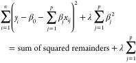where y_i refers to a given observation, out of n observations. β₀ is the ordinate at the origin, it corresponds to the average value of the response variable y when all predictors are zero. β_j is the average effect that the increase in one unit of the predictor variable (in this case, wavenumber) x_j, (j ∈ {0 ... p}) has on the response variable, keeping the rest of the variables constant. They are known as partial regression coefficients.

The main advantage of applying ridge over adjustment by OLS is the reduction of variance. In general, in situations where the relationship between the response variable and the predictors is approximately linear, least-squares estimates have little bias but can still suffer from high variance (small changes in the training data have a large impact on the resulting model). This problem is accentuated as the number of predictors introduced in the model approaches the number of training observations, reaching the point where, if p > n, it is not possible to fit the model by ordinary least-squares. Using a suitable value of λ, the ridge method is capable of reducing variance without hardly increasing the bias, thus achieving a lower total error.

The disadvantage of the ridge method is that the final model includes all of the predictors. This is so because although the penalty forces the coefficients to approach zero, they never reach exactly zero (only if λ = ∞). This method manages to minimize the influence on the model of the predictors less related to the response variable.

Multivariate analyses were performed using Scikit-learn: Machine Learning in Python⁵⁶ using learn.linear_model.Ridge. We found an optimal ridge λ of 0.0035 by using the grid search technique.⁵⁷ For evaluation we used 5-fold cross-validation. Additional confirmatory analyses by PLS-DA were performed using Pirouette (Infometrix, Bothell, WA, USA).

Results and Discussion

SARS-CoV-2 Infection Status

Averaged Spectra of Both Categories (SARS-CoV-2 Infected and Non-infected)

In Figure 1, the average of all 55 SARS-CoV-2 positive spectra and the average of all 194 negatives are shown. The following wavenumbers/regions showed apparent differences between both types of spectra (cm^–1): 550–650; 1000–1160; band around 1232; band around 1300; band around 1394; band around 1492; band around 1635; band around 1714; band around 2898; 2917–2960; band around 3056; and band around 3274. Since these spectra averages reflect contributions by all of the compounds present within the sera (where proteins, cholesterol, urea, and triglycerides, among other more diluted compounds, can be found, plus additional contributions by viral infection),¹⁹ spectra are similar, thus the need for additional tools in order to establish a model that would allow for separation into categories.

Figure 1.

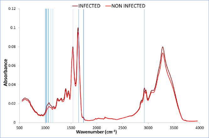
Average of all 55 SARS-CoV-2 positive spectra, and the average of all 194 negatives (cm^–1). Wavenumbers selected for separation of categories between both types of samples indicated by vertical lines.

Chemometric Processing of Spectra

Correlation-based feature subset selection²⁸ was used to find the relevant wavenumbers that allow for separation into SARS-CoV-2 infected and non-infected categories. This algorithm evaluates the worth of a subset of attributes by considering the individual predictive ability of each feature along with the degree of redundancy between them. The search method was bidirectional bestfirst. Twenty-five wavenumbers were selected out of 1,718. Selected wavenumbers are shown in Table 1 and Figure 1.

Table 1. Wavenumbers Selected by Our Model for Separation in Categories between SARS-CoV-2 Infected and Non-infected Patients (cm^–1).

1018.23	1045.22	1054.87	1079.94	1643.05
1024.01	1047.15	1068.37	1116.58	1646.91
1025.94	1049.08	1070.29	1135.86	1751.04
1027.87	1051.01	1076.08	1159.00	1752.97
1035.58	1052.94	1078.01	1536.98	2923.55

Additional confirmatory analyses by PLS-DA were performed, using Pirouette software, on the sera spectra data matrix built with the wavenumbers selected by the previously developed model based on correlation-based subset selection algorithm for segregating in categories between SARS-CoV-2 infected and non-infected patients (wavenumbers as listed in Table 1). In Figure 2, the 2D graphical representation of Y1/CS1 (dependent variable 1/class specific result 1) scores obtained by PLS-DA are presented. Red diamonds correspond to infected patients, whereas brown diamonds correspond to non-infected patients. A clear, although overlapping separation in a cluster for the SARS-CoV-2 infected group, is observed in Figure 2.

Figure 2.

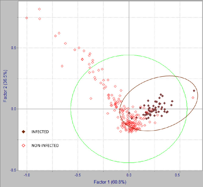
2D representation of Y1/CS1 scores by PLS-DA of SARS-CoV-2 infected and non-infected patients.

Spectral Interpretation and Band Assignments

Following infection by SARS-CoV-2 and during development of COVID-19 disease, several alterations in sera, measurable by IR, thus reflected in the spectra, may occur. On one hand, the spectral contribution by the virus itself, where 1657, 1547, and 1517 cm^–1 bands may be attributed to proteins (from spike, envelope, membrane, and nucleocapsid proteins), 1740, 1464, 1382, and 1341 cm^–1 bands may be attributed to lipids (from lipid bilayer surrounding the nucleocapsid), and 1690, 1235, 1124, 1089, 996, and 967 cm^–1 bands may be attributed to viral RNA; on the other hand, the host organism response to the virus infection, especially immune response, may also be observed, and thus, several biomarkers have been suggested for identifying SARS-CoV-2 infection.^18−21,58

Wavenumber shifts in bands attributed to a specific compound/family of compounds normally considered as sera components have been reported between infected and non-infected patients.¹⁹ Besides, some variations regarding the specific wavenumbers attributable to a given compound/family of compounds can be found between the studies performed by different authors.^18−21,58 Moreover, it has been reported that several factors may influence the quality of IR spectra which may cause distortion (for example, unfolding, conformational changes, and denaturation that proteins may suffer after exposure to high temperatures).¹⁹ Therefore, as it has been suggested by the authors, the exact biological interpretation of those bands involved in SARS-CoV-2/COVID-19 status assessment by infrared spectroscopy may require further experimental confirmation in future studies.⁵⁸

Regarding wavenumbers selected by our model for separation in categories between SARS-CoV-2 infected and non-infected patients, those in the range between 1100 and 850 cm^–1 may be attributed to nucleic acids; it is a region where, in their work, authors reported a higher expression in the COVID-19 group.²⁰ Within the region, specifically bands at 1028 and 1037 cm^–1 (1036 cm^–1 in our work) may be correlated to contributions by glycogen (since it is known that the SARS-CoV-2 spike glycoprotein—S-protein—has 66 glycosilation sites which may be occupied by glycans upon infection).²⁰ Bands at 1068 and 1070 cm^–1 may correspond to C–O stretching in ribose.¹⁸ The band at 1076 cm^–1, explained by symmetrical stretching vibrations of PO₂^– phosphodiester groups, has shown an increase in SARS-CoV-2 groups.¹⁹⁻²¹ Bands at 1117 and 1080 cm^–1 may be related to viral RNA (the latter, specifically to symmetric PO₂^– stretching).^18,21 The band at 1537 cm^–1 may be attributed to amide II (mainly in-plane N–H bending), whereas bands at 1643 and 1647 cm^–1 to amide I (mainly stretching vibrations of C=O as well as C–N groups) absorption bands of proteins. The band at 1159 cm^–1 may be explained by C–O–C symmetric stretching of phospholipids, triglycerides, and cholesterol esters.¹⁹ Since overlapping of contributions by different functional groups may occur (especially given the complexity of sera composition), additional sources may contribute to specific bands within the spectra. The range between 1160 and 1028 cm^–1 has been attributed to IgM, whereas the range between 1560 and 1028 cm^–1, to IgA.²⁰

Comparison with Cytokine Standards

Cytokine storm, where an aggressive inflammatory response by the host occurs, mediated by pro-inflammatory cytokines, has been reported as an aggravating factor related to COVID-19 disease. It is a hyperactive response which leads to an excessive inflammatory reaction that has been directly correlated with lung injury, multiorgan failure, and unfavorable prognosis of severe COVID-19.⁵⁹⁻⁶² Elevated levels of cytokines in COVID-19 infected patients, when compared to healthy adults, have been reported in several studies. Huang et al.⁵⁹ reported that the initial plasma IL1B, IL1RA, IL7, IL8, IL9, IL10, basic FGF, GCSF, GMCSF, IFNγ, IP10, MCP1, MIP1A, MIP1B, PDGF, TNFα, and VEGF concentrations were higher in both ICU patients and non-ICU patients than in healthy adults. Further comparison between ICU and non-ICU patients showed that plasma concentrations of IL2, IL7, IL10, GCSF, IP10, MCP1, MIP1A, and TNFα were higher in ICU patients than non-ICU patients. Chen et al.⁶² reported that serum levels of interleukin 2R (IL-2R), IL-6, IL-10, and tumor necrosis factor α (TNF-α) were markedly higher in severe cases than in moderate cases. And Liu et al.⁶³ found a significant increase of IL-6 levels correlated to the clinical manifestation of severe patients. Immune response related to SARS-CoV-2 infection, disease development and vaccination, has been also investigated by infrared spectroscopy and multivariate analysis. Bandeira et al.⁶⁴ studied structural changes in IgG induced by COVID-19 by FTIR and PLS-DA; and Dogan et al.⁶⁵ were able to successfully separate in categories vaccinated from nonvaccinated patients by ATR-FTIR, PCA, and LDA analysis of sera.

In this work, we analyzed the following cytokine standards: IL-1, IL-1α, IL-1β, IL-2, IL-6, IL-17 (although not listed in the aforementioned studies, it is a pro-inflammatory cytokine which has been suggested as a possible target for immunomodulatory treatment of COVID-19),⁶⁶ TNF-α, IFN-γ, CXCL10 (also known as interferon γ induced protein 10; IP-10), and VEGF. Regarding correspondences between cytokine standards absorption bands and wavenumbers selected by our model for separation in SARS-CoV-2 infected and non-infected categories, there was observed a correspondence in several wavenumbers; thus, alterations in cytokine blood levels upon infection could also be contributing to changes in the serum spectra from infected patients when compared to those from healthy individuals. In Table 2 we present a correlation between wavenumbers selected for separation in SARS-CoV-2 infected vs non-infected patients as selected by our model (as shown in Table 1) and absorption maximum bands of cytokine standards analyzed in this study (the raw spectra are shown in Figure 3).

Table 2. Maximum Bands of Cytokine Standards Wavelengths vs SARS-CoV-2 Contagion Selected Wavelengths (cm^–1).

IP-10	VEGF	IL-6	IL-2	IFN-γ	IL-1α	IL-1	IL-1β	TNF-α	IL-17	selected λ
1069										1068, 1070
			1117							1117
					1076	1076		1077		1076, 1078
							1080			1080
1538	1538	1542			1542	1540		1536		1537
	1644					1643	1642	1642	1641	1643
1648		1649	1648		1649		1646			1647

Figure 3.

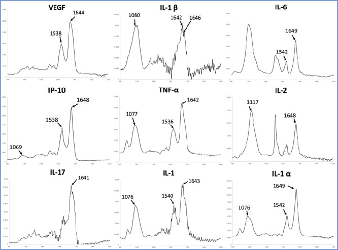
Raw spectra of cytokine standards where correspondence with our model was shown (in absorbance vs wavenumber range in cm^–1).

Validity

Using wavenumbers listed in Table 1, the classifier was able to correctly classify 242 instances, leaving only 7 incorrectly classified ones. This corresponds to 97.19% instances being correctly classified. Confusion matrix for SARS-CoV-2 infection status instances classification is shown in Table 3.

Table 3. Confusion Matrix for SARS-CoV-2 Infection Status Instances Classification.

cohorts	non-infected	SARS-CoV-2 infected
negatives	190	4
positives	3	52

According to Table 3, 52 samples are considered as TP and 190 as TN, four samples were incorrectly classified as positives (FP), and three were incorrectly classified as negatives (FN).

Therefore, for separation in categories between SARS-CoV-2 infected and non-infected patients in this study, sensitivity is 94.55% and specificity is 98.44%. Table 4 shows precision, recall, F-measure, Matthews correlation coefficient, ROC, and precision-recall curves area per class.

Table 4. Evaluation Matrix for SARS-CoV-2 Infection Status Classification.

class	precision	recall	F-measure	MCC	ROC area	PRC area
non-infected	0.984	0.979	0.982	0.919	0.949	0.962
infected	0.929	0.945	0.937	0.919	0.895	0.488
weighted average	0.972	0.972	0.972	0.919	0.937	0.858

COVID-19 Disease Severity Status

Data Processing

We used raw infrared absorbance data from the 249 samples, as described earlier, and considered the following COVID-19 severity status cohorts: not infected, mild, severe, and severity unknown, based on SARS-CoV-2 infected patients’ clinical history, plus additional information regarding the samples. The distribution of cases is shown in Table 5.

Table 5. Distribution of Cases.

severity	cases
not infected	194
unknown	12
high	31
mild	12

A new model was built using attribute selection, as described earlier, for achieving separation in categories according to COVID-19 disease severity status on the 249 sera samples data matrix. Out of 1,718 wavenumbers, 14 wavenumbers were selected for this model (Table 6).

Table 6. Wavenumbers Selected by Our Model for Assessing COVID-19 Disease Severity (cm^–1).

1014.37	1051.01	1083.79	2792.42
1031.72	1052.94	1646.91	2923.55
1039.44	1054.87	1756.83
1049.08	1064.51	2391.29

Spectral Interpretation, Band Assignments, and Correlation to Cytokine Standards

The following wavenumbers selected by or model for assessing COVID-19 disease severity were also selected for differentiation in categories between SARS-CoV-2 infected and non-infected patients (cm^–1): 1049, 1051, 1053, 1055, 1065, 1647, and 2924. Therefore, discussion regarding those wavenumbers was previously presented. Wavenumbers 1014, 1032, 1039, and 1084 cm^–1 are within the range 1100–850 cm^–1, reported as a region for nucleic acids. More specifically, bands at 1032 and 1039 cm^–1 may be correlated to contributions by glycogen.²⁰ The band at 1084 may be related to viral RNA (symmetric PO₂^– stretching) (Zhang et al.¹⁹ report a range between 1083 and 1086 cm^–1). The band at 1757 cm^–1 is within the reported range for the amide I absorption band of proteins.²⁰ Regarding correlation to cytokine standards, only 1647 cm^–1 corresponds to absorption maximum bands of IP-10 (1648 cm^–1), IL-6 (1649 cm^–1), IL-1α (1649 cm^–1), and IL-1β (1646 cm^–1).

Validity

Pursuant to their clinical history, 31 patients presented severe COVID-19 disease, thus leaving 218 samples regarded as not severe. Twelve patients were affected with mild COVID-19; therefore, 237 were regarded as not mild. Besides, 12 patients among those positive for SARS-CoV-2 contagion were unknown regarding COVID-19 severity status (it is worth noting that we are discarding any possible bias that could be introduced by these samples, since no status regarding this topic could be assumed in this case).

According to Table 7, 33 instances were classified as severe, where 22 belonged to the high-severity cohort; nine were incorrectly classified as severe, and 11 were incorrectly classified as not severe. Sixteen samples were classified as mild, where four belonged to the mild severity cohort, 8 were incorrectly classified as mild, and 12 were incorrectly classified as not mild.

Table 7. Confusion Matrix for COVID-19 Disease Severity.

	classification according to model
cohorts (according to clinical history)	not infected	unknown	severe	mild
not infected	186	2	1	5
severity unknown	2	0	8	2
severe	1	3	22	5
mild	4	2	2	4

According to the formulas previously described, the results for assessing the severity of COVID-19 disease in this study are as follows: For severe disease classification, sensitivity is 70.97%, and specificity is 94.95%. For mild disease classification, sensitivity is 33.33% and specificity 94.93%.

It is important to mention that additional samples with the complete information regarding COVID-19 severity status should be analyzed in the future for improving the robustness of the model, as well as the biological understanding based on spectral bands assignments. However, the potential of ATR-FTIR and chemometrics analysis of serum samples for assessing COVID-19 severity status was observed in this work.

Dengue Infection Status

Although it was not the main objective of this work, considering that some of the samples were classified as “dengue positive”, we decided to extract the maximum information from the data set; thus, we evaluated the data obtained from all of the processed spectra for assessing status regarding dengue contagion. Since we lack information regarding the dengue positive samples, notably, the serotype of the dengue virus involved, we believe that it would be a stretch to attempt to form a biological explanation through spectral interpretation.

Data Processing

For dengue infection status assessment, serum spectra from the 322 samples originally processed were considered, since the lack of information regarding SARS-CoV-2 infection status on the 73 samples discarded for the two previous models do not affect cohorts in this case. Therefore, out of 322 samples, 75 were infected with dengue, while 247 were considered as non-infected with dengue. It is important to note that although the same raw infrared absorbance data were used, dengue and SARS-CoV-2 sets were disjointed. Using the previously presented method for feature selection, a new model was built, where 24 wavenumbers were selected (out of 1,718) (see Table 8).

Table 8. Wavenumbers Selected by Our Model for Separation in Categories between Dengue Infected and Non-infected Patients (cm^–1).

1008.58	1556.27	2285.23	2902.34
1012.44	1558.20	2289.09	2925.48
1024.01	1724.04	2387.44	3394.10
1351.85	1725.97	2389.37	3561.87
1365.35	1754.90	2391.29	3727.72
1554.34	2273.66	2412.51	3789.43

Validity

Using the wavenumbers listed in Table 6, the classifier was able to correctly classify 294 instances, leaving 28 incorrectly classified (accuracy of 91.304%). The confusion matrix for dengue infection status instances classification is presented in Table 9.

Table 9. Confusion Matrix for Dengue Infection Status Instances Classification.

	classification according to model
cohorts	non-infected	infected with dengue
non-infected	233	14
infected with dengue	14	61

According to the confusion matrix shown in Table 7, there were 61 TP, 233 TN, 14 FN, and 14 FP. Thus, according to formulas (as described before), for separation in categories between dengue infected and non-infected patients in this study, sensitivity is of 81.33% and specificity is of 94.33%. Table 10 shows precision, recall, F-measure, Matthews correlation coefficient, ROC, and precision-recall curves area per class.

Table 10. Evaluation Matrix for Dengue Infection Status Classification.

class	precision	recall	F-measure	MCC	ROC area	PRC area
non-infected	0.936	0.943	0.940	0.737	0.943	0.982
infected	0.808	0.787	0.797	0.737	0.943	0.858
weighted average	0.913	0.913	0.913	0.737	0.943	0.953

More studies should be performed on this topic, although the potential of ATR-FTIR and chemometrics for identifying dengue contagion status in serum was observed in this work. It is worth mentioning that other colleagues have also successfully used ATR-FTIR for identifying dengue virus contagion.^17,67,68

Conclusions

In this work, we corroborated the potential of ATR-FTIR and chemometrics for assessing SARS-CoV-2 contagion status, as reported by colleagues in previous works.^18−21,58 Several serum constituents including viral RNA, proteins, glycogen, antibodies, and cytokines, could be attributed to differences in the infrared spectra between infected and non-infected patients, thus serving as chemical fingerprints. High sensitivity (94.55%) and high specificity (98.44%) were achieved by our model for separating into categories sera samples with regard to SARS-CoV-2 infection status. The low TATs plus the simplicity of sample preparation and infrared analysis, which could be performed by clinical laboratory personnel, followed by multivariate analysis, which could be performed via cloud computing, are promising for the development of a widespread rapid SARS-CoV-2 testing tool. As specifically investigated in this work, given the correspondence between cytokines absorption bands and wavenumbers selected by our model for distinguishing between infected and non-infected patients, alterations in cytokine blood levels upon infection could be related to changes in infected patients’ serum infrared spectra, thus reflecting the influence of pro-inflammatory cytokines in COVID-19 disease development.

Assessing COVID-19 severity by analyzing infected patients’ sera samples with a rapid, low-cost technique, such as ATR-FTIR and multivariate analysis, would help medical personnel to prioritize severe patients in a timely manner, thus potentially reducing fatalities from COVID-19 disease, as well as a better management of generally reduced resources within the currently overwhelmed healthcare infrastructure. According to our model, for separating in categories regarding COVID-19 severity status, for severe disease classification, sensitivity is 70.97%, and specificity is 94.93%. For mild disease classification, sensitivity is 33.33% and specificity 94.93%. It is worth noting that further investigation should be performed in order to improve the robustness of the model, as well as for determining spectral contributions upon disease development with higher precision.

Another advantage of ATR-FTIR and chemometrics analysis of sera samples include the possibility for developing models for extracting additional information from the same data matrix. Regarding dengue contagion status, according to our model, sensitivity is of 81.33%, and specificity is of 94.33%.

In summary, we have shown the potential of ATR-FTIR followed by multivariate analysis for the developing of a rapid and low-cost SARS-CoV-2 infection status and COVID-19 severity diagnostic tool, which can also assess other viruses that may be present within the samples.

Author Contributions

^∇ O.C.-G. and H.C. contributed equally to this work.

The authors declare no competing financial interest.

References

- Bryant P.; Elofsson A. Estimating the impact of mobility patterns on COVID-19 infection rates in 11 European countries. Peer J. 2020, 8, e9879 10.7717/peerj.9879. [DOI] [PMC free article] [PubMed] [Google Scholar]
- Li T.; Liu Y.; Li M.; Qian X.; Dai S. Y. Mask or no mask for COVID-19: A public health and market study. PLoS One 2020, 15, e0237691. 10.1371/journal.pone.0237691. [DOI] [PMC free article] [PubMed] [Google Scholar]
- Ağalar C.; Ozturk Engin D. Protective measures for COVID-19 for healthcare providers and laboratory personnel. Turk. J. Med. Sci. 2020, 50, 578–584. 10.3906/sag-2004-132. [DOI] [PMC free article] [PubMed] [Google Scholar]
- Pouwels K. B.; et al. Effect of Delta variant on viral burden and vaccine effectiveness against new SARS-CoV-2 infections in the UK. Nat. Med. 2021, 27, 2127–2135. 10.1038/s41591-021-01548-7. [DOI] [PMC free article] [PubMed] [Google Scholar]
- Nepogodiev D.; Bhangu A.; Glasbey J. C.; Li E.; Omar O. M.; Simoes J. F.; Abbott T. E.; Alser O.; Arnaud A. P.; Bankhead-Kendall B. K.; et al. Mortality and pulmonary complications in patients undergoing surgery with perioperative SARS-CoV-2 infection: an international cohort study. Lancet 2020, 396, 27–38. 10.1016/S0140-6736(20)31182-X. [DOI] [PMC free article] [PubMed] [Google Scholar]
- Tsai S.; Lu C.; Bau D.; Chiu Y.; Yen Y.; Hsu Y.; Fu C.; Kuo S.; Lo Y.; Chiu H.; Juan Y.; Tsai F.; Yang J. Approaches towards fighting the COVID-19 pandemic (Review). Int. J. Mol. Med. 2020, 47, 3–22. 10.3892/ijmm.2020.4794. [DOI] [PMC free article] [PubMed] [Google Scholar]
- Nitin P.; Nandhakumar R.; Vidhya B.; Rajesh S.; Sakunthala A. COVID-19: Invasion, pathogenesis and possible cure – A review. J. Virol. Methods 2022, 300, 114434. 10.1016/j.jviromet.2021.114434. [DOI] [PMC free article] [PubMed] [Google Scholar]
- Means A. R.; Wagner A. D.; Kern E.; Newman L. P.; Weiner B. J. Implementation Science to Respond to the COVID-19 Pandemic. Front. Public Health 2020, 8, 462. 10.3389/fpubh.2020.00462. [DOI] [PMC free article] [PubMed] [Google Scholar]
- Vandenberg O.; Martiny D.; Rochas O.; van Belkum A.; Kozlakidis Z. Considerations for diagnostic COVID-19 tests. Nat. Rev. Microbiol. 2021, 19, 171–183. 10.1038/s41579-020-00461-z. [DOI] [PMC free article] [PubMed] [Google Scholar]
- Lai C. K. C.; Lam W. Laboratory testing for the diagnosis of COVID-19. Biochem. Biophys. Res. Commun. 2021, 538, 226–230. 10.1016/j.bbrc.2020.10.069. [DOI] [PMC free article] [PubMed] [Google Scholar]
- Sun X.; Wang T.; Cai D.; Hu Z.; Chen J.; Liao H.; Zhi L.; Wei H.; Zhang Z.; Qiu Y.; Wang J.; Wang A. Cytokine storm intervention in the early stages of COVID-19 pneumonia. Cytokine Growth Factor Rev. 2020, 53, 38–42. 10.1016/j.cytogfr.2020.04.002. [DOI] [PMC free article] [PubMed] [Google Scholar]
- Pokhrel P.; Hu C.; Mao H. Detecting the Coronavirus (COVID-19). ACS Sens 2020, 5, 2283–2296. 10.1021/acssensors.0c01153. [DOI] [PMC free article] [PubMed] [Google Scholar]
- Pray I. W.; et al. Performance of an antigen-based test for asymptomatic and symptomatic SARS-CoV-2 testing at two university campuses—Wisconsin, September–October 2020. Morb. Mortal. Wkly. Rep. 2021, 69, 1642–1647. 10.15585/mmwr.mm695152a3. [DOI] [PMC free article] [PubMed] [Google Scholar]
- Zhao J.; et al. Antibody Responses to SARS-CoV-2 in Patients With Novel Coronavirus Disease 2019. Clin. Infect. Dis. 2020, 71, 2027–2034. 10.1093/cid/ciaa344. [DOI] [PMC free article] [PubMed] [Google Scholar]
- Böger B.; Fachi M. M.; Vilhena R. O.; Cobre A. F.; Tonin F. S.; Pontarolo R. Systematic review with meta-analysis of the accuracy of diagnostic tests for COVID-19. Am. J. Infect. Control 2021, 49, 21–29. 10.1016/j.ajic.2020.07.011. [DOI] [PMC free article] [PubMed] [Google Scholar]
- Roy S.; Perez-Guaita D.; Andrew D. W.; Richards J. S.; McNaughton D.; Heraud P.; Wood B. R. Simultaneous ATR-FTIR Based Determination of Malaria Parasitemia, Glucose and Urea in Whole Blood Dried onto a Glass Slide. Anal. Chem. 2017, 89, 5238–5245. 10.1021/acs.analchem.6b04578. [DOI] [PubMed] [Google Scholar]
- Santos M. C. D.; Nascimento Y. M.; Araújo J. M. G.; Lima K. M. G. ATR-FTIR spectroscopy coupled with multivariate analysis techniques for the identification of DENV-3 in different concentrations in blood and serum: a new approach. RSC Adv. 2017, 7, 25640–25649. 10.1039/C7RA03361C. [DOI] [Google Scholar]
- Barauna V. G.; Singh M. N.; Barbosa L. L.; Marcarini W. D.; Vassallo P. F.; Mill J. G.; Ribeiro-Rodrigues R.; Campos L. C. G.; Warnke P. H.; Martin F. L. Ultrarapid On-Site Detection of SARS-CoV-2 Infection Using Simple ATR-FTIR Spectroscopy and an Analysis Algorithm: High Sensitivity and Specificity. Anal. Chem. 2021, 93, 2950–2958. 10.1021/acs.analchem.0c04608. [DOI] [PubMed] [Google Scholar]
- Zhang L.; Xiao M.; Wang Y.; Peng S.; Chen Y.; Zhang D.; Zhang D.; Guo Y.; Wang X.; Luo H.; Zhou Q.; Xu Y. Fast Screening and Primary Diagnosis of COVID-19 by ATR–FT-IR. Anal. Chem. 2021, 93, 2191–2199. 10.1021/acs.analchem.0c04049. [DOI] [PubMed] [Google Scholar]
- Martinez-Cuazitl A.; Vazquez-Zapien G. J.; Sanchez-Brito M.; Limon-Pacheco J. H.; Guerrero-Ruiz M.; Garibay-Gonzalez F.; Delgado-Macuil R. J.; de Jesus M. G. G.; Corona-Perezgrovas M. A.; Pereyra-Talamantes A.; Mata-Miranda M. M. ATR-FTIR spectrum analysis of saliva samples from COVID-19 positive patients. Sci. Rep. 2021, 11, 19980. 10.1038/s41598-021-99529-w. [DOI] [PMC free article] [PubMed] [Google Scholar]
- Wood B. R.; Kochan K.; Bedolla D. E.; Salazar-Quiroz N.; Grimley S.; Perez- Guaita D.; Baker M. J.; Vongsvivut J.; Tobin M.; Bambery K.; et al. Infrared based saliva screening test for COVID-19. Angew. Chem. 2021, 60, 17102. 10.1002/anie.202104453. [DOI] [PMC free article] [PubMed] [Google Scholar]
- Nascimento M. H. C.; Marcarini W. D.; Folli G. S.; da Silva Filho W. G.; Barbosa L. L.; Paulo E. H.; Vassallo P. F.; Mill J. G.; Barauna V. G.; Martin F. L.; de Castro E. V. R.; Romao W.; Filgueiras P. R. Noninvasive Diagnostic for COVID-19 from Saliva Biofluid via FTIR Spectroscopy and Multivariate Analysis. Anal. Chem. 2022, 94, 2425–2433. 10.1021/acs.analchem.1c04162. [DOI] [PubMed] [Google Scholar]
- Guleken Z.; Jakubczyk P.; Wieslaw P.; Krzysztof P.; Bulut H.; Oten E.; Depciuch J.; Tarhan N. Characterization of Covid-19 infected pregnant women sera using laboratory indexes, vibrational spectroscopy, and machine learning classifications. Talanta 2022, 237, 122916. 10.1016/j.talanta.2021.122916. [DOI] [PMC free article] [PubMed] [Google Scholar]
- Nogueira M. S.; Leal L. B.; Marcarini W. D.; Pimentel R. L.; Muller M.; Vassallo P. F.; Campos L. C. G.; Dos Santos L.; Luiz W. B.; Mill J. G.; Barauna V. G.; de Carvalho L. F. D. C. E. S. Rapid diagnosis of COVID-19 using FT-IR ATR spectroscopy and machine learning. Sci. Rep. 2021, 11, 15409. 10.1038/s41598-021-93511-2. [DOI] [PMC free article] [PubMed] [Google Scholar]
- Shlomo I. B.; Frankenthal H.; Laor A.; Greenhut A. K. Detection of SARS-CoV-2 infection by exhaled breath spectral analysis: Introducing a ready-to-use point-of-care mass screening method. EclinicalMedicine 2022, 45, 101308. 10.1016/j.eclinm.2022.101308. [DOI] [PMC free article] [PubMed] [Google Scholar]
- Kitane D. L.; Loukman S.; Marchoudi N.; Fernandez-Galiana A.; El Ansari F. Z.; Jouali F.; Badir J.; Gala J. L.; Bertsimas D.; Azami N.; Lakbita O.; Moudam O.; Benhida R.; Fekkak J. A simple and fast spectroscopy-based technique for Covid-19 diagnosis. Sci. Rep. 2021, 11, 16740. 10.1038/s41598-021-95568-5. [DOI] [PMC free article] [PubMed] [Google Scholar]
- Lee L. C.; Liong C.-Y.; Jemain A. A. Partial least squares-discriminant analysis (PLS-DA) for classification of high-dimensional (HD) data: a review of contemporary practice strategies and knowledge gaps. Analyst 2018, 143, 3526–3539. 10.1039/C8AN00599K. [DOI] [PubMed] [Google Scholar]
- Hall M. A.; Smith L. A.. Practical feature subset selection for machine learning. 1998.
- Darnell M. E.; Taylor D. R. Evaluation of inactivation methods for severe acute respiratory syndrome coronavirus in noncellular blood products. Transfusion 2006, 46, 1770–7. 10.1111/j.1537-2995.2006.00976.x. [DOI] [PMC free article] [PubMed] [Google Scholar]
- Cameron J. M.; Butler H. J.; Anderson D. J.; Christie L.; Confield L.; Spalding K. E.; Finlayson D.; Murray S.; Panni Z.; Rinaldi C.; Sala A.; Theakstone A. G.; Baker M. J. Exploring pre-analytical factors for the optimization of serum diagnostics: Progressing the clinical utility of ATR-FTIR spectroscopy. Vib. Spectrosc. 2020, 109, 103092. 10.1016/j.vibspec.2020.103092. [DOI] [Google Scholar]
- Liu Y.; Yu X.; Huang J. X.; An A. Combining integrated sampling with SVM ensembles for learning from imbalanced datasets. Inf. Process. Manage. 2011, 47, 617–631. 10.1016/j.ipm.2010.11.007. [DOI] [Google Scholar]
- Hastie T.; Tibshirani R.; Friedman J. H.; Friedman J. H.. The elements of statistical learning: Data mining, inference, and prediction, 2nd ed.; Springer, 2009; Vol. 2. [Google Scholar]
- Hilbe J. M.Logistic regression models; Chapman and Hall/CRC, 2009. [Google Scholar]
- Kleimbaum D. G.; Kupper L. L.; Muller K. E.; Nizam A.. Applied regression analysis and multivariable methods, 4th ed.; Duxbury Press, 2007. [Google Scholar]
- Karsmakers P.; Pelckmans K.; Suykens J. A.. Multi-class kernel logistic regression: a fixed-size implementation. 2007 International Joint Conference on Neural Networks; IEEE, 2007; pp 1756–1761. 10.1109/IJCNN.2007.4371223. [DOI] [Google Scholar]
- Hosmer D. W.; Lemeshow S.; Cook E.. Applied logistic regression, 2nd ed.; John Wiley and Sons: New York, 2000. 10.1002/0471722146. [DOI] [Google Scholar]
- Komarek P.; Moore A. W.. Making logistic regression a core data mining tool with TR-IRLS. Fifth IEEE International Conference on Data Mining (ICDM’05); IEEE, 2005, pp 1−4. 10.1109/ICDM.2005.90. [DOI] [Google Scholar]
- Lin C.-J.; Weng R. C.; Keerthi S. S. Trust region Newton method for large-scale logistic regression. J. Mach. Learn. Res. 2008, 9, 627–650. [Google Scholar]
- Koh K.; Kim S.-J.; Boyd S. An interior-point method for large-scale l1-regularized logistic regression. J. Mach. Learn. Res. 2007, 8, 1519–1555. [Google Scholar]
- King G.; Zeng L. Logistic regression in rare events data. Political analysis 2001, 9, 137–163. 10.1093/oxfordjournals.pan.a004868. [DOI] [Google Scholar]
- Blum A.; Langley P. Selection of relevant features and examples in machine learning. Artif. Intell. 1997, 97, 245–271. 10.1016/S0004-3702(97)00063-5. [DOI] [Google Scholar]
- Dash M.; Liu H. Feature selection for classifications. Intell. Data Anal. 1997, 1, 131–156. 10.1016/S1088-467X(97)00008-5. [DOI] [Google Scholar]
- Kohavi R.; John G. Wrappers for feature subset selection. Artif. Intell. 1997, 97, 273–324. 10.1016/S0004-3702(97)00043-X. [DOI] [Google Scholar]
- Xing E.; Jordan M.; Karp R.. Feature selection for high-dimensional genomic microarray data. Proceedings of the Eighteenth International Conference on Machine Learning; Morgan Kaufmann: San Francisco, CA, USA, 2001; pp 601–608.
- Yang Y.; Pederson J.. A comparative study on feature selection in text categorization. Proceedings of the Fourteenth International Conference on Machine Learning; Morgan Kaufmann: San Francisco, CA, USA, 1997; pp 412–420.
- Rui Y.; Huang T.; Chang S. Image retrieval: Current techniques, promising directions and open issues. J. Visual Commun. Image Represent. 1999, 10, 39–62. 10.1006/jvci.1999.0413. [DOI] [Google Scholar]
- Ng K.; Liu H. Customer retention via data mining. Artif. Intell. Rev. 2000, 14, 569–590. 10.1023/A:1006676015154. [DOI] [Google Scholar]
- Liu H.; Motoda H.; Yu L.. Feature Selection for Knowledge Discovery and Data Mining; Kluwer, 2002. [Google Scholar]
- Das S.Filters, wrappers and a boosting-based hybrid for feature selection. Proceedings of the Eighteenth International Conference on Machine Learning; Morgan Kaufmann: San Francisco, CA, USA, 2001; pp 74–81.
- Mitra P.; Murthy C.; Pal S.. Unsupervised feature selection using feature similarity. IEEE Transactions on Pattern Analysis and Machine Intelligence; IEEE, 2002; Vol. 24, pp 301–312. 10.1109/34.990133. [DOI]
- Das S. Feature selection with a linear dependence measure. IEEE Trans. Comput. 1971, C-20, 1106–1109. 10.1109/T-C.1971.223412. [DOI] [Google Scholar]
- Quinlan J. R. C4.5: Programs for machine learning. Mach. Learn. 1993, 16, 235–240. 10.1007/BF00993309. [DOI] [Google Scholar]
- Martin F. L.; Kelly J. G.; Llabjani V.; Martin-Hirsch P. L.; Patel I. I.; Trevisan J.; Fullwood N. J.; Walsh M. J. Distinguishing cell types or populations based on the computational analysis of their infrared spectra. Nat. Protoc. 2010, 5, 1748–60. 10.1038/nprot.2010.133. [DOI] [PubMed] [Google Scholar]
- Le Cessie S.; Van Houwelingen J. C. Ridge estimators in logistic regression. J. R. Stat. Soc., Ser. C 1992, 41, 191–201. 10.2307/2347628. [DOI] [Google Scholar]
- Bühlmann P.; Van De Geer S.. Statistics for high-dimensional data: methods, theory and applications; Springer Science & Business Media, 2011. 10.1007/978-3-642-20192-9. [DOI] [Google Scholar]
- Pedregosa F.; Varoquaux G.; Gramfort A.; Michel V.; Thirion B.; Grisel O.; Blondel M.; Prettenhofer P.; Weiss R.; Dubourg V.; et al. Scikit-learn: Machine learning in Python. J. Mach. Learn. Res. 2011, 12, 2825–2830. [Google Scholar]
- Rao C. R.; Rao A. S. S.. Data Science: Theory and Applications; Handbook of Statistics, Vol. 44; Elsevier, 2021. [Google Scholar]
- Banerjee A.; Gokhale A.; Bankar R.; Palanivel V.; Salkar A.; Robinson H.; Shastri J. S.; Agrawal S.; Hartel G.; Hill M. M.; Srivastava S. Rapid Classification of COVID-19 Severity by ATR-FTIR Spectroscopy of Plasma Samples. Anal. Chem. 2021, 93, 10391–10396. 10.1021/acs.analchem.1c00596. [DOI] [PubMed] [Google Scholar]
- Huang C.; Wang Y.; Li X.; Ren L.; Zhao J.; Hu Y.; Zhang L.; Fan G.; Xu J.; Gu X.; et al. Clinical features of patients infected with 2019 novel coronavirus in Wuhan, China. Lancet 2020, 395, 497–506. 10.1016/S0140-6736(20)30183-5. [DOI] [PMC free article] [PubMed] [Google Scholar]
- Ragab D.; Salah Eldin H.; Taeimah M.; Khattab R.; Salem R. The COVID-19 Cytokine Storm; What We Know So Far. Front. Immunol. 2020, 11, 1446. 10.3389/fimmu.2020.01446. [DOI] [PMC free article] [PubMed] [Google Scholar]
- Ruan Q.; Yang K.; Wang W.; Jiang L.; Song J. Clinical predictors of mortality due to COVID-19 based on an analysis of data of 150 patients from Wuhan, China. Intensive Care Med. 2020, 46, 846–848. 10.1007/s00134-020-05991-x. [DOI] [PMC free article] [PubMed] [Google Scholar]
- Chen G.; et al. Clinical and immunological features of severe and moderate coronavirus disease 2019. J. Clin. Investig. 2020, 130, 2620–2629. 10.1172/JCI137244. [DOI] [PMC free article] [PubMed] [Google Scholar]
- Liu T.; Zhang J.; Yang Y.; Ma H.; Li Z.; Zhang J.; Cheng J.; Zhang X.; Zhao Y.; Xia Z.; Zhang L.; Wu G.; Yi J.. The potential role of IL-6 in monitoring severe case of coronavirus disease 2019. medRxiv Preprint (Infectious Diseases (except HIV/AIDS)), 2020. https://doi.org/10.1101/2020.03.01.20029769.
- Bandeira C. C. S.; Madureira K. C. R.; Rossi M. B.; Gallo J. F.; da Silva A. P. M. A.; Torres V. L.; de Lima V. A.; Junior N. K.; Almeida J. D.; Zerbinati R. M.; Braz-Silva P. H.; Lindoso J. A. L.; da Silva Martinho H. Micro-Fourier-transform infrared reflectance spectroscopy as tool for probing IgG glycosylation in COVID-19 patients. Sci. Rep. 2022, 12, 4269. 10.1038/s41598-022-08156-6. [DOI] [PMC free article] [PubMed] [Google Scholar]
- Dogan A.; Gurbanov R.; Severcan M.; Severcan F. CoronaVac (Sinovac) COVID-19 vaccine-induced molecular changes in healthy human serum by infrared spectroscopy coupled with chemometrics. Turk. J. Biol. 2021, 45, 549–558. 10.3906/biy-2105-65. [DOI] [PMC free article] [PubMed] [Google Scholar]
- Pacha O.; Sallman M. A.; Evans S. E. COVID-19: a case for inhibiting IL-17?. Nat. Rev. Immunol. 2020, 20, 345–346. 10.1038/s41577-020-0328-z. [DOI] [PMC free article] [PubMed] [Google Scholar]
- Naseer K.; Ali S.; Qazi J. ATR-FTIR spectroscopy based differentiation of typhoid and dengue fever in infected human sera. Infrared Phys. Technol. 2021, 114, 103664. 10.1016/j.infrared.2021.103664. [DOI] [PubMed] [Google Scholar]
- Ali S.; Naseer K.; Hussain I.; Qazi J. ATR-FTIR spectroscopy-based differentiation of hepatitis C and dengue infection in human freeze-dried sera. Infrared Phys. Technol. 2021, 118, 103912. 10.1016/j.infrared.2021.103912. [DOI] [Google Scholar]