LARGE-SCALE MULTIVARIATE SPARSE REGRESSION WITH APPLICATIONS TO UK BIOBANK

Abstract

In high-dimensional regression problems, often a relatively small subset of the features are relevant for predicting the outcome, and methods that impose sparsity on the solution are popular. When multiple correlated outcomes are available (multitask), reduced rank regression is an effective way to borrow strength and capture latent structures that underlie the data. Our proposal is motivated by the UK Biobank population-based cohort study, where we are faced with large-scale, ultrahigh-dimensional features, and have access to a large number of outcomes (phenotypes)—lifestyle measures, biomarkers, and disease outcomes. We are hence led to fit sparse reduced-rank regression models, using computational strategies that allow us to scale to problems of this size. We use a scheme that alternates between solving the sparse regression problem and solving the reduced rank decomposition. For the sparse regression component we propose a scalable iterative algorithm based on adaptive screening that leverages the sparsity assumption and enables us to focus on solving much smaller subproblems. The full solution is reconstructed and tested via an optimality condition to make sure it is a valid solution for the original problem. We further extend the method to cope with practical issues, such as the inclusion of confounding variables and imputation of missing values among the phenotypes. Experiments on both synthetic data and the UK Biobank data demonstrate the effectiveness of the method and the algorithm. We present multiSnpnet package, available at http://github.com/junyangq/multiSnpnet that works on top of PLINK2 files, which we anticipate to be a valuable tool for generating polygenic risk scores from human genetic studies.

1. Introduction.

The past two decades have witnessed rapid growth in the amount of data available to us. Many areas such as genomics, neuroscience, economics, and Internet services have been producing increasingly larger datasets that have high dimension, large sample size, or both. A variety of statistical methods and computational tools have been developed to accommodate this change so that we are able to extract valuable information and insight from these massive datasets (Hastie, Tibshirani and Friedman (2009), Efron and Hastie (2016), Dean and Ghemawat (2008), Zaharia et al. (2010), Abadi et al. (2016)).

One major motivating application for this work is the study of data from population-scale cohorts like UK Biobank with genetic data from over one million genetic variants and phenotype data from thousands of phenotypes in over 500,000 individuals (Bycroft et al. (2018)). These data present unprecedented opportunities to explore very comprehensive genetic relationships with phenotypes of interest. In particular, the subset of tasks we are interested in is the prediction of a person’s phenotype value, such as disease affection status, based on his or her genetic variants.

Genome-wide association studies (GWAS) is a very powerful and widely used framework for identifying genetic variants that are associated with a given phenotype; see, for example, Visscher et al. (2017) and the references therein. It is based on the results of univariate marginal regression over all candidate variants and tries to find a subset of significant ones. While being computationally efficient and easy to interpret, GWAS has fairly limited prediction performance because at most one predictor can present in the model. If prediction performance is our main concern, it is natural to consider the class of multivariate methods that considers multiple variants simultaneously. In the past, wide data were prevalent where only a limited number, like thousands, of samples were available. In this regime some sophisticated multivariate methods could be applicable, though they have to more or less deal with dimension reduction or variable selection. In this setting we handle hundreds of thousands samples and even more variables. In such cases, statistical methods and computational algorithms become equally important because only efficient algorithmic design will allow for the application of sophisticated statistical modeling. Recently, we introduced some algorithms addressing these challenges. In particular, Qian et al. (2020) proposed an iterative screening framework that is able to fit the exact lasso/elastic-net solution path in large-scale and ultrahigh-dimensional settings and demonstrate competitive computational efficiency and superior prediction performance over previous methods.

In this paper we consider the scenarios where multivariate responses are available in addition to the multiple predictors and propose a suite of statistical methods and efficient algorithms that allow us to further improve the statistical performance in this large n and large p regime. Some characteristics we want to leverage and challenges we want to solve include:

1. Statistics. There are thousands of phenotypes available in the UK Biobank. Many of them are highly correlated with each other and can have a lot of overlap in their driving factors. By treating them separately, we lose this information that could have been used to stabilize our model estimation. The benefit of building a joint model can be seen from the following simplified model. Suppose all the outcomes y^k, k = 1, …, q are independent noisy observations of a shared factor u = Xβ such that y^k = u + e^k. It is easy to see that by taking an average across all the outcomes, we obtain a less noisy response $\overline{y}$, and this will give us more accurate parameter estimation and better prediction than the model built on any of the single outcome. The assumption of such latent structure is an important approach to capturing the correlation structure among the outcomes and can bring in a significant reduction in variance if the data indeed behave in a similar way. We will formalize this belief and build a model on top of it. In addition, in the presence of high-dimensional features, we will follow the “bet on sparsity” principle (Hastie, Tibshirani and Friedman (2009)) and assume that only a subset of the predictors are relevant to the prediction.

   Therefore, the statistical model we will build features two major assumptions: low-rank in the signal and sparse effect. Furthermore, we will introduce integrated steps to systematically deal with confounders and missing values.

2. Computation. On a large-scale dataset, building a multivariate model can pose great computational challenges. For example, loading the entire UK Biobank dataset into memory with double precision will take more than one terabyte of space, while typically most existing statistical computing tools assume that the data are already sitting in memory. Even if large memory is available, one can always encounter data or construct features so that it becomes insufficient. Hence, instead of expecting sufficient memory space, we would like to find a scalable solution that is less restricted by the size of physical memory.

There is a dynamic data-access mechanism provided by the operating system, called memory mapping (Bovet and Cesati (2005)), that allows for easy access to larger-than-memory data on the disk. In essence, it carries a chunk of data from disk to memory when needed and swap some old chunks of data out of memory when it is full. In principle, we could add a layer of memory mapping on top of all the procedures and then access the data as if they were in memory. However, there is one important practical component that should never be ignored: disk I/O. This is known to be expensive in the operating system and can greatly delay the computation if frequent disk I/Os are involved. For this reason, we do not pursue first-order gradient-based methods, such as stochastic gradient descent (Bottou (2010)) or dual averaging (Xiao (2010), Duchi, Agarwal and Wainwright (2012)), because it can take a large number of passes over the data for the objective function to converge to the optimum.

To address this, we design the algorithm so that it needs as few full passes over the data as possible while solving the exact objective. In particular, by leveraging the sparsity assumption we propose an adaptive screening approach that allows us to strategically select a small subset of variables into memory, do intensive computation on the subset, and then verify the validity of all the left-out variables. The last step is important because we want to guarantee that the solution obtained from the algorithm is a valid solution to the original full problem.

1.1. Reduced-rank regression for multiple responses.

In the standard multivariate linear regression model, given a model matrix $X=\left(x_1,\dots ,x_p\right)\in {ℝ}^{n\times p}$ and a multivariate response matrix $Y=\left(y_1,\dots ,y_q\right)\in {ℝ}^{n\times q}$, we assume that

$$Y=XB+E,$$

where each row of E = (e₁, …, e_q) is assumed to be an independent sample from some multivariate Gaussian distribution $E^{(i)}\stackrel{\text{iid}}{~}𝒩\left(0,{\Sigma }_E\right)$. When n ≥ q, it is easy to see that an maximum likelihood estimator (MLE) can be found by solving a least squares problem with multiple outcomes, that is,

$$\widehat{B}\in \underset{B\in {ℝ}^{p\times q}}{\text{argmin}}\frac{1}{2}\Vert Y-XB{\Vert }_F^2,$$ (1.1)

where $\Vert A{\Vert }_F^2={\sum }_{i=1}^n{\sum }_{j=1}^m{A}_{ij}^2$ is the squared Frobenius norm of a matrix $A\in {ℝ}^{n\times m}$. When n ≥ p and X has full rank, (1.1) has the closed-form solution $\widehat{B}={\left(X^{\top }X\right)}^{-1}{X}^{\top }Y$. Notice that this is equivalent to solving q single-response regression problems separately.

However, in many scenarios there can be some correlation structure in the signals that we can capture to improve the statistical efficiency of the estimator. One approach to modeling the correlation is to assume that there is a set of latent factors that act as the drivers for all the outcomes. When we assume that the dependencies of the latent factors on the raw features and the outcomes on the latent factors are both linear, it is equivalent to making a low-rank assumption on the coefficient matrix. Reduced-rank regression (Anderson (1951), hereafter RRR) assumes that the coefficient matrix B has a fixed rank r ≤ min(p, q), or

$$B=U{V}^{\top },$$

where $U=\left(u_1,\dots ,u_r\right)\in {ℝ}^{p\times r}$, $V={\left(v_1,\dots ,v_q\right)}^{\top }\in {ℝ}^{q\times r}$.¹ With the decomposed coefficient matrices an alternative way to express the multivariate model is to assume that there exists a set of latent factors $\left\{z_{\ell }\in {ℝ}^n:1\le \ell \le r\right\}$ such that, for each ℓ,

$$z_{\ell }=X{u}_{\ell },$$

$$y_k=Z{v}_k+e_k.$$

Figure 1 gives a visualization of the dependency structure described above. It can also be seen as a a multilayer perceptron (MLP) with linear activation and one hidden layer or multitask learning with bottleneck. We notice that, under the decomposition, the parameters are not identifiable. In fact, if we apply any nonsingular linear transformation $M\in {ℝ}^{r\times r}$ such that V′ = VM^⊤ and U′= UM⁻¹, it yields the same model but different parameters. As a result, we also have an infinite number of MLEs.

Fig. 1.

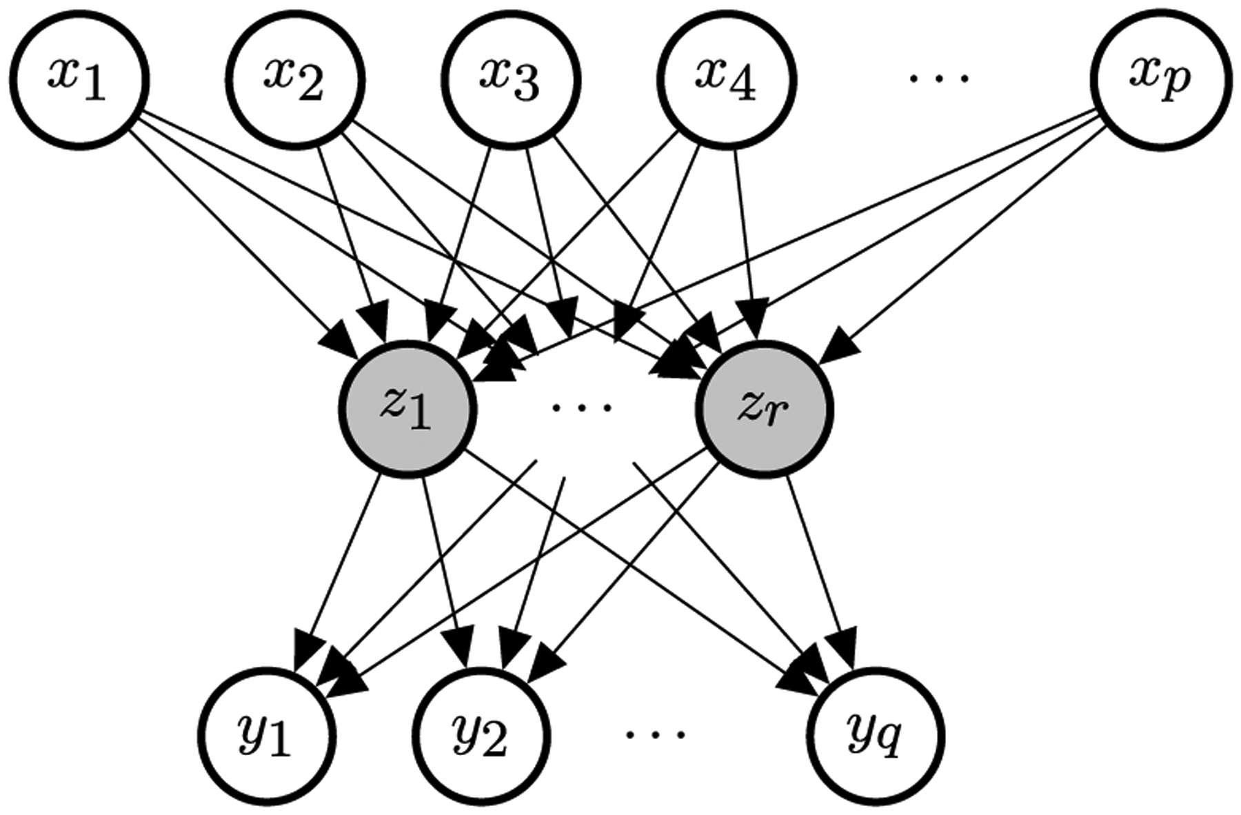
Diagram of the reduced-rank regression. The nodes in grey are latent variables. The arrows represent the dependency structure. Known as multitask learning in the machine learning community.

Under the rank constraint, an explicit global solution can be obtained. Let MDN^⊤ be the singular value decomposition (SVD) of ${\left(X^{\top }X\right)}^{-\frac{1}{2}}{X}^{\top }Y$, a set of solution is given by $\widehat{U}={\left(X^{\top }X\right)}^{-1}{X}^{\top }YN$, $\widehat{V}=N$. Reinsel and Velu (1998) has a comprehensive discussion on the model under classical large n settings.

1.2. Sparse models in high-dimensional problems.

In the setting of high-dimensional problems where p > n, the original low-rank coefficient matrix B can be unidentifiable. Often, sparsity is assumed in the coefficients to model the belief that only a subset of the features are relevant to the outcomes. To find such a sparse estimate of the coefficients, a widely used approach is to add an appropriate nonsmooth penalty to the original objective function to encourage the desired sparsity structure. Common choices include the lasso penalty (Tibshirani (1996)), the elastic-net penalty (Zou and Hastie (2005)), or the group lasso penalty (Yuan and Lin (2006)). There has been a great amount of work studying the consistency of estimation and model selection under such settings; see Bach (2008), Bickel, Ritov and Tsybakov (2009), Bühlmann and van de Geer (2011), Greenshtein and Ritov (2004), Meinshausen and Bühlmann (2006), Obozinski, Wainwright and Jordan (2011), Wainwright (2009), Zhao and Yu (2006) and references therein. In particular, the group lasso, as the name suggests, encourages group-level sparsity induced by the following penalty term:

$$P_g(\beta )=\sum _{j=1}^J{\Vert {\beta }_j\Vert }_2,$$

where ${\beta }_j\in {ℝ}^{p_j}$ is the subvector corresponding the j th group of variables and ${\Vert {\beta }_j\Vert }_2=\sqrt{{\sum }_{\ell =1}^{p_j}{\beta }_{j,\ell }^2}$ is the vector ℓ₂-norm. The ℓ₂-norm enforces that if the fitted model has ${\Vert {\widehat{\beta }}_j\Vert }_2=0$, all the elements in ${\widehat{\beta }}_j$ will be 0, and otherwise, with probability one, all the elements will be nonzero. This yields a desired group-level selection in many applications. Throughout the paper we will adopt the group lasso penalty, defining each predictor’s coefficients across all outcomes as a distinct group, in order to achieve homogeneous sparsity across multiple outcomes. In addition to variable selection for better prediction and interpretation, we will also see the computational advantages we leverage to develop an efficient algorithm.

2. Sparse reduced-rank regression.

Given a rank r, we are going to solve the following penalized rank-constrained optimization problem:

$$\begin{array}{l}\text{minimize}\frac{1}{2}\Vert Y-XB{\Vert }_F^2+\lambda \sum _{j=1}^p{\Vert B_{j\cdot }\Vert }_2,\\ \text{s}.\text{t}.\hspace{1em}\text{rank}(B)\le r.\end{array}$$ (2.1)

Alternatively, we can decompose the matrix explicitly as B = UV^⊤, where $U\in {ℝ}^{p\times r}$, $V\in {ℝ}^{q\times r}$. It can be shown that the problem above is equivalent to the sparse reduced-rank regression (SRRR) proposed by Chen and Huang (2012),

$$\begin{array}{l}\text{minimize}\frac{1}{2}{\Vert Y-XU{V}^{\top }\Vert }_F^2+\lambda \sum _{j=1}^p{\Vert U_j\Vert }_2,\\ \text{s}.\text{t}.V^{\top }V=I\text{. }\end{array}$$ (2.2)

Alternating minimization was proposed by Chen and Huang (2012) to solve this nonconvex optimization problem, where two algorithms were considered: subgradient descent and a variational method. The subgradient method was shown to be faster when p ≫ n and the variational method faster when n ≫ p. However, in each iteration, the computational complexity of either method is at least quadratic in the number of variables p. It makes the problem almost intractable in ultrahigh-dimensional problems, which is common, for example, in modern genetic studies. Moreover, to obtain a model with good prediction performance, we are interested in solving the problem over multiple λ’s rather than a single one. For such purposes, we design a path algorithm with adaptive variable screening that will be both memory and computationally efficient.

We note that (2.2) is a nonconvex optimization problem. Although the algorithm we propose next is to solve (2.2) exactly, we do not claim the solution we obtain to be any of the local minima or global minima—a property nice to have but cannot be easily guaranteed in general. The subgradient descent or variational method does not offer this guarantee. We will show later that, under some regularity conditions, the solution will be optimal, but in general, it is a limiting point of the some alternating minimization scheme. For convenience, in the rest of the paper, when we say a valid or exact solution to the original problem, we mean it is a limiting point of the proposed scheme. That being said, we will show empirically that the solution found by the algorithm is usually reasonably good on the landscape.

3. Fast algorithms for large-scale and ultrahigh-dimensional problems.

First, we present a naive version of the path solution which will be the basis of our subsequent development. The path is defined on a decreasing sequence of λ values λ_max = λ₁ > λ₂ > ⋯ > λ_L ≥ 0, where λ_max is often defined by one that leads to the trivial (e.g., all zero) solution and the rest are often determined by an equally spaced array on the log scale. In particular, for Problem (2.1) we are able to figure out the exact lower bound of λ_max for which the solution is trivial.

Lemma 3.1. In problem (2.1), if r > 0, the maximum λ that results in a nontrivial solution $\widehat{B}(\lambda )$ is

$${\lambda }_{\text{max}}=\underset{1\le j\mid \le p}{\text{max}}{\Vert x_j^{\top }Y\Vert }_2.$$

The proof is straightforward, which is a result of the Karush–Kuhn–Tucker (KKT) condition (see Boyd and Vandenberghe (2004) for more details). We present the full argument in the Supplementary Material B (Qian et al. (2022)). The naive path algorithm tries to solve the problem independently across different λ values.

3.1. Alternating minimization.

The algorithm is described in Algorithm 1. For each value of λ in a predefined sequence λ₁ > ⋯ > λ_L ≥ 0, it applies alternating minimization to Problem (2.2) until convergence.

In the V-step (3.1), we will be solving the orthogonal Procrustes problem, given a fixed U^(k). An explicit solution can be constructed from the singular value decomposition, as detailed in the following Lemma.

Lemma 3.2. Suppose p ≥ r and $Z\in {ℝ}^{p\times r}$. Let Z = MDN^⊤ be its singular value decomposition, where $M\in {ℝ}^{p\times r}$, $D\in {ℝ}^{r\times r}$ and $N\in {ℝ}^{r\times r}$. An optimal solution to

$$\underset{V\in {ℝ}^{p\times r}:V^{\top }V=I}{\text{maximize}}\text{Tr}\left(Z^{\top }V\right)$$

is given by $\widehat{V}=M{N}^{\top }$, and the objective function has optimal value ∥Z∥_*, the nuclear norm of Z. When Z has full rank, the solution is unique.

Proof. See in Supplement B (Qian et al. (2022)). □

To analyze the computational complexity of the algorithm, we see a one-time computation of Y^⊤X that costs O(npq). In each iteration there is O(pqr) complexity for the matrix multiplication Y^⊤XU^(k) and O(qr²) for computing the SVD and the final solution. Therefore, the per-iteration computational complexity for the V-step is O(pqr + qr²), or O(pqr) when p ≫ q.

In the U-step, we are solving a group lasso problem. Computing YV^(k+1) takes O(nqr) time. The group-lasso problem can be solved by glmnet (Friedman, Hastie and Tibshirani (2010)) with the mgaussian family. With coordinate descent, its complexity is $O(\tilde{k}pqn)$, where $\tilde{k}$ is the number of iterations until convergence and is expected to be small with a reasonable initialization, for example, provided by warm start. Thus, the per-iteration complexity for the U-step is $O(nqr+\tilde{k}npq)$ which is $O(\tilde{k}pqn)$ when p ≫ r.

Therefore, the overall computational complexity scales, at least linearly, with the number of features and will have a large multiplier if the sample size is large as well. While subsampling can effectively reduce the computational cost, in high-dimensional settings it is critical to have sufficient samples for the quality of estimation. Instead, we seek for computational techniques that can lower the actual number of features involved in expensive iterative computation without giving up any statistical efficiency. Thanks to the induced sparsity by the objective function, we are able to achieve it by variable screening.

3.2. Variable screening for ultrahigh-dimensional problems.

In this section we discuss strategic ways to find a good subset of variables to focus on in the computation that would allow us to reconstruct the full solution easily. In particular, we would like to iterate through the following steps for each λ:

1. Screen a strong set S, and treat all the left-out variables S^c as null variables that potentially have zero coefficients;

2. Solve a significantly smaller problem on the subset of variables S;

3. Check an optimality condition to guarantee the constructed full solution $\widehat{B}=\left({\widehat{B}}_S,{\widehat{B}}_{S^c}\right)$ with ${\widehat{B}}_{S^c}=0$ is indeed a valid solution to the original problem. If the condition is not satisfied, go back to the first step with an expanded set S.

3.2.1. Screening strategies.

We have seen Lemma 3.1 that determines the entry point of any nonzero coefficient on the solution path. Furthermore, there is evidence that the variables entering the model (as one decreases the λ value) tend to have large values by this criterion. Tibshirani et al. (2012) developed on this idea and proposed the strong rules as a sequential variable screening mechanism. The strong rules state that in a standard lasso problem with the model matrix $X=\left(x_1,\dots ,x_p\right)\in {ℝ}^{n\times p}$ and a single response $y\in {ℝ}^n$, assume $\widehat{\beta }\left({\lambda }_{k-1}\right)$ is the lasso solution at λ_k−1; then, the j th predictor is discarded at λ_k if

$$\left|x_j^{\top }\left(y-X\widehat{\beta }\left({\lambda }_{k-1}\right)\right)\right|<{\lambda }_k-\left({\lambda }_{k-1}-{\lambda }_k\right).$$ (3.3)

The key idea is that the inner product above is almost “nonexpansive” in terms of λ. As a result, the KKT condition suggests that the variables to be discarded by (3.3) would have coefficient 0 at λ_k. However, it is not a guarantee. The strong rules can fail, though failures occur rarely when p > n. In any case, the KKT condition is checked to ensure the exact solution is found. Although Tibshirani et al. (2012) focused mostly on the lasso-type problem, they also suggested extension to general objective functions and penalties. For general objective function f(β) with p_j-norm penalty ∥β_j∥_pj for the j th group, the screening criterion will be based on the dual norm of its gradient ∥∇_jf(β)∥q_j, where 1/p_j + 1/q_j = 1.

Inspired by the general strong rules, we propose three sequential screening strategies for the sparse reduced rank objective (2.2), named after their respective characteristics: Multi-Gaussian, Rank-Less and Fix-V. They are based either on the solution of a relaxed convex problem at the same λ_k or on the exact solution at the previous λ_k−1:

1. (Multi-Gaussian) Solve the full-rank convex problem at λ_k, and use its active set as the candidates for the low-rank settings. The main advantage is that the screening is always stable, due to the convexity. However, this approach often overselects and brings extra burden to the computation. By assuming a higher rank than necessary, the effective number of responses would become more than that of a low-rank model. As a result, more variables would potentially be needed to serve for an enlarged set of responses.

2. (Rank-Less) Find variables that have large $c_j={\Vert X_j^T\left(Y-XU\left({\lambda }_{k-1}\right)V{\left({\lambda }_{k-1}\right)}^{\top }\right)\Vert }_2$. This is analogous to the strong rules applied to the vanilla multiresponse lasso, ignoring the rank constraint.

3. (Fix-V) Find variables that have large $c_j^{\prime }={\Vert X_j^T\left(YV\left({\lambda }_{k-1}\right)-XU\left({\lambda }_{k-1}\right)\right)\Vert }_2$. This is similar to the strong rules applied in the U-step with V assumed fixed. To see the rationale better, we take another perspective. The squared error in SRRR (2.2) can also be written as

   $${\Vert Y-XU{V}^{\top }\Vert }_F^2=\mathbf{\text{Tr}}\left(Y^{\top }Y\right)-2\mathbf{\text{Tr}}\left(Y^{\top }XU{V}^{\top }\right)+\mathbf{\text{Tr}}\left(XU{V}^{\top }V{U}^{\top }{X}^{\top }\right).$$

Since V^⊤V = I, the optimization problem becomes

$$\underset{U,V:V^{\top }V=I}{\text{minimize}}\frac{1}{2}\Vert XU{\Vert }_F^2-Tr\left(Y^{\top }XU{V}^{\top }\right)+\lambda \sum _{j=1}^p{\Vert U_{j.}\Vert }_2.$$

For any given U, we can solve V = MN^⊤, where Y^⊤XU = MDN^⊤ is its singular value decomposition. Let $f(U)=\frac{1}{2}\Vert XU{\Vert }_F^2-{\Vert Y^{\top }XU\Vert }_{*}$. The problem is reduced to

$$\underset{U}{\text{minimize}}f(U)+\lambda \sum _{j=1}^p{\Vert U_j\cdot \Vert }_2.$$

The general strong rule suggests that we screen based on the gradient (or subgradient if Y^⊤XU is not full rank); that is,

$${\nabla }_{U}f(U)=X^{\top }XU-X^{\top }YM{N}^{\top }=X^{\top }(XU-YV).$$

Therefore, the general strong rules endorse the use of this screening rule.

We do some experiments to compare the effectiveness of the rules. We simulate the model matrix under an independent design and an equicorrelated design with correlation ρ = 0.5. The exact solution path is computed using Algorithm 1 with several random initializations and the convex relaxation-based initialization (as in the multi-Gaussian rule). Let S(λ) be the true active set at λ. For each method ℓ above, we can find, based on either the exact solution at λ_k−1 or the full-rank solution at λ_k, the threshold it needs so that, by the screening criterion, the selected subset $\widehat{S}{\left({\lambda }_k\right)}^{(\ell )}$ contains the true subset at λ_k, that is, $\widehat{S}{\left({\lambda }_k\mid {\lambda }_{k-1}\right)}^{(\ell )}\supseteq S\left({\lambda }_k\right)$. This demonstrates how deep each method has to search down the variable list to include all necessary variables and thus how accurate the screening mechanism is—the smaller the subset, the better the method. Figure 2 shows an example scenario with problem size n = 200, p = 500, q = 20, and k = 20 nonzero rows of coefficients. The true rank is set to be 3 and signal-to-noise ratio (SNR) is 1. We compute the solution over 50 λ values equally spaced on the log-scale. Additional experiments are showed in the Supplementary Material D (Qian et al. (2022)).

Fig. 2.

Size of screened set under different strategies. Left: Independent design. Right: Equicorrelated design with ρ = 0.5. Size: n = 200, p = 500, q = 20, and k = 20 nonzero rows of coefficients. Signal-to-noise ratio (SNR) = 1, and we use the true rank = 3.

We see from both plots that the curve of the Fix-V method is able to track that of the exact subset fairly well, while the Rank-Less and Multi-Gaussian methods both choose a much larger subset in order to cover the full active set in the exact solution. In the rest of the paper, we will adopt the Fix-V method to do variable screening.

3.2.2. Optimality condition.

Although the Fix-V method turns out to be most effective in choosing the subset of variables, in practice, we have no access to the true subset and have to take an estimate. Instead of trying to find a sophisticated threshold, we will do batch screening at a fixed size (this size can change adaptively though). Given a size M, we will take the M variables that rank the top under this criterion. Clearly, we can make mistakes by having left out some important variables in the screening stage. In order to make sure that our solution is exact rather than approximate in terms of the original problem, we need to check the optimality condition and take in more variables when necessary.

Suppose we find a solution ${\widehat{U}}_S$, ${\widehat{V}}_S$ on a subset of variables X_S by alternating minimization. We will verify the assembled solution $\widehat{U}=\left({\widehat{U}}_S,0\right)$, $\widehat{V}={\widehat{V}}_S$ is a limit point of the original optimization problem. The argument is supported by the following lemma.

Lemma 3.3. In the U-step (3.2), given V and λ, if we have an exact solution ${\widehat{U}}_S$ for the sub-problem with X_S, then $\widehat{U}=\left({\widehat{U}}_S,0\right)$ is a solution to the full problem if and only if for all j ∈ S^c,

$${\Vert x_j^{\top }\left(YV-X_S{\widehat{U}}_S\right)\Vert }_2\le \lambda .$$ (3.4)

Proof. Since this is a convex problem, $\widehat{U}$ is a solution if and only if $0\in \partial f(\widehat{U})$ where f is the objective function in (3.2) and ∂f is its subdifferential. For the vector ℓ₂-norm, we know that the subdifferential of ∥x∥₂ is $\left\{s\in {ℝ}^p:\Vert s{\Vert }_2\le 1\right\}$ if x = 0 and {x/∥x∥₂} if x ≠ 0. Notice that $X_S{\widehat{U}}_S=X\widehat{U}$ by the definition of $\widehat{U}$. Since we have an exact solution on S, we know $0\in \partial f{(\widehat{U})}_j$. for all j ∈ S. On the other hand, for j ∈ S^c, $0\in \partial f(\widehat{U})$ if and only if $0\in \left\{x_j^{\top }(X\widehat{U}-YV)+\lambda s_j:{\Vert s_j\Vert }_2\le 1\right\}$ which is further equivalent to ${\Vert x_j^{\top }\left(YV-X_S{\widehat{U}}_S\right)\Vert }_2={\Vert x_j^{\top }(YV-X\widehat{U})\Vert }_2\le \lambda$ □

Therefore, once we obtain a solution ${\widehat{U}}_s$, ${\widehat{V}}_s$ for the subproblem and get condition (3.4) verified, we know in the V-step, by the lemma above, $\widehat{U}=\left({\widehat{U}}_S,0\right)$ is the solution given $\widehat{V}={\widehat{V}}_S$. In the U-step, since $X\widehat{U}=X_S{\widehat{U}}_S$, $\widehat{U}$ is the solution to the full problem. We see that $(\widehat{U},\widehat{V})$ is a limiting point of the alternating minimization algorithm for the original problem. However, if the condition fails, we expand the screened set or bring in the violated variables and do the fit again. As mentioned earlier, we do not guarantee the final solution to be a local minimum or global minimum, unless under some regularity conditions. It is instead a limiting point of the vanilla alternating minimization algorithm, that is, Algorithm 1. In other words, if we start from the constructed solution (with zero coefficients for the left-out variables), the algorithm should converge in one iteration and return the same solution.

We have seen the main ingredients of the iterative algorithm: screening, solving, and checking. Next, we discuss some useful practical considerations and extensions.

3.3. Computational considerations.

3.3.1. Initialization and warm start.

Recall that, in the training stage, our goal is to fit an SRRR solution path across different λ values. It is easy to see that, with a careful choice of parameterization, the path is continuous in λ. To leverage this property, we adopt a warm start strategy. Specifically, we initialize the coefficients of the existing variables at λ_k+1, using the solution at λ_k, and zero-initialize the newly added variables. With warm start, much less iterations will be needed to converge to the new minimum.

However, this by no means guarantees that we are all on a good path. It’s likely that we are trapped into a neighborhood of local optimum and end up with much higher function value than the global minimum. One way to alleviate this, if affordable, is to solve the corresponding full-rank problem first, and initialize the coefficients with low-rank approximation of the full-rank solution. We can compare the limiting function values with the warm-start initialization and see which converges to a better point. Although we didn’t use in the actual implementation and experiments, one could also do random exploration—randomly initialize some of the coefficients, run the algorithm multiple times, and find one that achieves the lowest function value. That said, we lose the advantage of warm start though. The good news is, in the experiments we have done, we didn’t observe very clear suboptimal behavior by the warm-start and full-rank strategies.

3.3.2. Size of expanded variable set.

As described above, when the KKT check fails, we expand the current screened set by adding more variables from the rest of the variables. In our framework the number of variables to add is a hyperparameter subject to the user’s choice. There is some computational tradeoff in determining the expansion size—the more variables one adds each time, the less likely that the KKT check will fail so as to call for another round of computation, but with a larger variable set, the per-round computation also scales up.

3.3.3. Early stopping.

Although we prespecify a sequence of λ values λ₁ > λ₂ > ⋯ > λ_L where we want to fit the SRRR models, we do not have to fit them all, given our goal is to find the best predictive model. Once the model starts to overfit as we move down the λ list, we can stop our process since the later models will have no practical use and are expensive to train. Therefore, in the actual computation, we monitor the validation error along the solution path and call it a stop if it shows a clear upward trend. One other point we would like to make in this regard is that the validation metric can be defined either as an average MSE over all phenotypes or a subset of phenotypes in which we are most interested. This is because practically the best λ value can be different for different phenotypes in the joint model.

3.4. Extensions.

On top of the core algorithm, we introduce several extensions that are lightweight but can be important for real-world applications, such as dealing with nonuniform scaling of the responses, existence of confounders, and missing data. In the Supplementary Material A (Qian et al. (2022)), we also introduce a weighting mechanism that allows one to encode priors on different responses.

3.4.1. Standardization.

We often want to standardize the predictors if they are not on the same scale because the penalty term is not invariant to change of units of the variables. However, we emphasize that some thought has to be put into this before standardizing the predictors. If the predictors are already on the same scale, standardizing them could bring unintended advantages to variables with smaller variance themselves. It is more reasonable not to standardize in such cases.

In terms of the outcomes, since they can be at different scales, it is important to standardize them in the training stage so that no one dominates in the objective function. At prediction (both training and test time), we scale back to the original levels using their respective variances from the training set. In fact, the real impact an outcome has to the overall objective is determined by the proportion of unexplained variance. It would be good to weight the responses properly based on this if such information is available or can be estimated, for example, via heritability estimation for phenotypes in genetic studies.

3.4.2. Adjustment covariates.

In some applications, such as genome-wide association studies (GWAS), there may be confounding variables $Z\in {ℝ}^{n\times m}$ that we want to adjust for in the model. For example, population stratification, defined as the existence of a systematic ancestry difference in the sample data, is one of the common factors in GWAS that can lead to spurious discoveries. This can be controlled for by including some leading principal components of the SNP matrix as variables in the regression (Price et al. (2006)). In the presence of such variables, we solve the following problem instead. With a slight abuse of notation, in this section, we use W to denote the coefficient matrix for the covariates instead of a weight matrix:

$$\begin{array}{l}\text{minimize}\frac{1}{2}{\Vert Y-ZW-XU{V}^{\top }\Vert }_F^2+\lambda \sum _{j=1}^p{\Vert U^j\Vert }_2,\\ \text{s}.\text{t}.V^{\top }V=I\text{.}\end{array}$$ (3.5)

The main components don’t change except two adjustments. When determining the starting λ value, we use Lemma 3.4.

Lemma 3.4. In problem (3.5), if r > 0, the maximum λ that results in a nontrivial solution $\widehat{B}(\lambda )$ is

$${\lambda }_{\text{max}}=\underset{1\le j\le p}{\text{max}}{\Vert x_j^{\top }\widehat{R}\Vert }_2,$$

where $\widehat{R}=Y-Z\widehat{W}$ and $\widehat{W}$ is the multiple outcome regression coefficient matrix.

The proof is almost the same as before. The other nuance we should be careful about is, when fitting the model, we should leave those covariates unpenalized because they serve for the adjustment purpose and should not be experiencing the selection stage. In particular, in the U-step (group lasso), given V, direct computation would reduce to solving the problem

$$\underset{U,W}{\text{minimize}}\frac{1}{2}\Vert YV-ZWV-XU{\Vert }_F^2+\lambda \sum _{j=1}^p{\Vert U^j\Vert }_2,$$

which is not as convenient as standard group lasso problem. Instead, we find that W can always be solved explicitly in terms of other variables. In fact, the minimizer of W is a least squares solution that can be expressed as $\widehat{W}={\left(Z^{\top }Z\right)}^{-1}{Z}^{\top }\left(Y-X{U}^{\top }\right)$. Plug in, and we find that the problem to be solved can be written as

$$\underset{U}{\text{minimize}}\frac{1}{2}{\Vert \left(I-H_Z\right)YV-\left(I-H_Z\right)XU\Vert }_F^2+\lambda \sum _{j=1}^p{\Vert U^j\Vert }_2,$$

where H_Z = Z(Z^⊤Z)⁻¹Z^⊤ is the projection matrix on the column space of Z. This becomes a standard group lasso problem and can be solved by using, for example, the glmnet package with the mgaussian family.

3.4.3. Missing values.

In practice, there can be missing values in either the predictor matrix or the outcome matrix. If we only discard samples that have any missing value, we could lose a lot of information. For the predictor matrix we could do imputation as simple as mean imputation or something sophisticated by leveraging the correlation structure. For missingness in the outcome, there is a natural way to integrate an imputation step seamlessly with the current procedure, analogous to the softImpute idea in Mazumder, Hastie and Tibshirani (2010). We first define a projection operator for a subset of two dimensional indices Ω ⊆ {1, …, n} × {1, …, p}. Let ${𝒫}_{\Omega }:{ℝ}^{n\times p}\to {ℝ}^{n\times p}$ be such that

$${𝒫}_{\Omega }{(Y)}_{i,j}=\{\begin{array}{ll}{Y}_{i,j},\hfill & (i,j)\in \Omega ,\hfill \\ 0,\hfill & (i,j)\notin \Omega .\hfill \end{array}$$

Let Ω be the set of indices where the response values are observed; in other words, Ω^c is the set of missing locations. Instead of (2.2), now we solve the following problem:

$$\begin{array}{l}\text{minimize}\frac{1}{2}{\Vert {𝒫}_{\Omega }(Y)-{𝒫}_{\Omega }\left(XU{V}^{\top }\right)\Vert }_F^2+\lambda \sum _{j=1}^p{\Vert U^j\Vert }_2,\\ \text{s}.\text{t}.V^{\top }V=I\text{.}\end{array}$$ (3.6)

We can easily see that an equivalent formulation of the problem is

$$\begin{array}{l}\underset{U,V,Y^{\prime }}{\text{minimize}}\frac{1}{2}{\Vert Y^{\prime }-XU{V}^{\top }\Vert }_F^2+\lambda \sum _{j=1}^p{\Vert U_{j.}\Vert }_2,\\ \text{s}.\text{t}.V^{\top }V=I,{𝒫}_{\Omega }\left(Y^{\prime }\right)={𝒫}_{\Omega }(Y)\text{.}\end{array}$$

This inspires a natural projection step to deal with the additional constraint. It can be well integrated with the current alternating minimization scheme. In fact, after each alternation between the U-step and the V-step, we can impute the missing values from the current predictions XUV^⊤ and then continue into the next U-V alternation with the completed matrix. This only adds computation in each iteration at a low cost of O(n|𝒜(λ)|rq), especially when the size of the screened set |𝒜(λ)| ≪ p which is common in practical high-dimensional applications.

3.4.4. Lazy reduced rank regression.

There is an alternative way to find a low-rank coefficient profile for the multivariate regression. Instead of pursing to solve the nonconvex problem (2.2) directly, we can follow a two-stage procedure:

1. Solve a full-rank multi-Gaussian sparse regression, that is,

   $${\text{minimize}}_B\frac{1}{2}\Vert Y-XB{\Vert }_F^2+\lambda \sum _{j=1}^p{\Vert B_j.\Vert }_2.$$

2. Conduct SVD of the resulting coefficient matrix $\widehat{B}$, and use its rank r approximation as our final estimator.

The advantage of this approach is that it is stable. The first stage is a convex problem and can be handled efficiently by, for example, glmnet. A variety of adaptive screening rules are also applicable in this situation to assist dimension reduction. The second stage is fairly standard and efficient as long as there are not too many active variables. However, the disadvantage is clear too. The low-rank approximation is conducted in an unsupervised manner and could lead to some degradation in the prediction performance.

That said, as before we should still evaluate the out-of-sample performance, as the penalty parameter λ varies and pick the best on the solution path as our final estimated model. In many cases where we compute the full-rank model under the exact mode anyways, the set of lazy models can be thought of as an efficient byproduct for our choice.

3.5. Full algorithm.

We incorporate the options above and present the full algorithm in Algorithm 2.

3.6. Memory and time costs.

Unlike most traditional procedures that need to operate on the full data, our SRRR algorithm takes advantage of sequential variable screening so that it restricts intensive computation on a small subsest of the variables. This makes it possible for memory-efficient implementations and also allows one to handle larger-than-RAM data.

In our Algorithm 2, variable screening and KKT Check will each incur one pass over the full data (that can, in fact, be merged into a single pass). We don’t have to bring all into memory but can instead use techniques, such as memory mapping, to deal with it efficiently. Since we will iterate over the candidate active set from screening multiple times, we often choose to explicitly load them into memory, and this will be the most memory expensive part. We will need, at most, O(n(|𝒜| + M)) space to save the set, where 𝒜 is the current active set and M is the size of the additional variables to be brought in from screening. That being said, in sparse ultrahigh-dimensional problems where we often expect |𝒜| ≪ p, our screening-based approach can greatly reduce the memory demand.

For each iteration, the computational complexity of variable screening is O(npq + nr(|𝒜(λ)| + q)), or O(npq) if |𝒜(λ)|, q ≪ p. However, the majority of this computation is independent for each variable and highly parallelizable. The actual computation time can be greatly reduced if we have access to multicore machines. The cost of alternating minimization depends on the actual number of iterations, which in turn depends on the initialization. This is why warm start can really help in computing the solution path. Down to each alternation, it takes O(nr(|𝒜| + q) + qr² + κn|𝒜|r) to compute, assuming that we use coordinate descent, and it takes κ steps to solve the group lasso problem (as glmnet does). We note that κ is often very small (e.g., 2–5) when we use warm start for the group lasso as well. After taking into account the number of alternating iterations K, the overall computational cost for solving one cycle of variable screening, alternating minimization, and KKT Check is O(npq) (parallelizable) + O(n|𝒜|rq) + O(K(nr(|𝒜| + q) + qr² + κn|𝒜|r)). If we further assume r, q ≪ |𝒜|, n, this cost becomes O(npq) (parallelizable) + O((K · κ + q)nr |𝒜|).

Therefore, the total computational cost of the algorithm scales linearly in the (average) per-cycle cost, or $O(\mathit{\text{Rnpq}})(\text{parallelizable})+O(R(K\cdot \kappa +q)nr|\overline{𝒜}|)$, depending on the potential number R of such cycles that is further determined by the number of repetitions per λ (due to KKT failure) and early stopping.

4. Convergence analysis.

In this section, we present some convergence properties of the alternating minimization algorithm (Algorithm 1) on sparse reduced rank regression. Let

$$g(U,V)=\frac{1}{2}{\Vert Y-XU{V}^{\top }\Vert }_F^2+\lambda \sum _{j=1}^p{\Vert U^j\Vert }_2.$$

Theorem 4.1. For any k ≥ 1, the function values are monotonically decreasing,

$$g\left(U^k,V^k\right)\ge g\left(U^{k+1},V^k\right)\ge g\left(U^{k+1},V^{k+1}\right).$$

Furthermore, we have the following finite convergence rate,

$$\underset{{}_{1\le k\le K}}{\text{min}}g\left(U^k,V^k\right)-g\left(U^{k+1},V^{k+1}\right)\le \frac{1}{K}\left(g\left(U^1,V^1\right)-g^{\infty }\right),$$

where g^∞ = lim_k→∞ g(U_k, V_k). It implies that the iteration will terminate in O(1/ϵ) iterations.

The proof is straightforward, and we won’t detail here. It presents the fact that alternating minimization is a descent algorithm. In fact, this property holds for all alternating minimization or more general blockwise coordinate descent algorithms. However, it does not say how good the limiting point is. In the next result, we show a local convergence result that, under some regularity conditions, if the initialization is closer enough to a global minimum, it will converge to a global minimum at linear rate. It is based on similar results on proximal gradient descent by Dubois, Delmas and Obozinski (2019). To define a local neighborhood, it would be easier if we eliminate V by always setting it to a minimizer given U. That is, by the second part of Lemma 3.2, at the optimal of V, the cross-term (in a trace form) coming from the expansion of the squared difference can be reduced to a nuclear norm, and thus the objective function becomes $F_{\lambda }(U)=\frac{1}{2}\Vert XU{\Vert }_2^2-{\Vert Y^{\top }XU\Vert }_{*}+\lambda {\sum }_{j=1}^p{\Vert U_{j.}\Vert }_2$. We define a sublevel set ${𝒮}_c(\lambda )=\left\{U\in {ℝ}^{p\times r}:F_{\lambda }(U)\le c\right\}$.

Theorem 4.2. Assume X^⊤X is invertible and ${\sigma }_{\text{max}}^2\ge {\sigma }_{\text{min}}^2>0$ be its smallest and largest eigenvalues. Let s_j be the j th singular value of ${\left(X^{\top }X\right)}^{-\frac{1}{2}}{X}^{\top }Y$. There exists $\overline{\lambda }>0$ such that, for all $0\le \lambda <\overline{\lambda }$ and $0\le \mu <{\sigma }_{\text{max}}^2\left(1-s_{r+1}^2/s_r^2\right)$, there is a sublevel set 𝒮(λ, μ) where the level depends on λ and μ such that, if U^k ∈ 𝒮(λ, μ), we have

$$\Delta \left(U^{k+1},V^{k+1}\right)\le \left(1-\text{min}\left(\frac{1}{2},\frac{\mu }{{\sigma }_{\text{max}}^2}\right)\right)\Delta \left(U^k,V^k\right),$$

where Δ(U, V) = g(U, V) − g(U*, V*) and (U*, V*) is a global minimum.

From a high level the proof is based on the fact that, under the conditions, the function is strongly convex near the global minima. If we start from this region, we achieve good convergence rate with alternating minimization algorithm. The full proof is given in the Supplementary Material B (Qian et al. (2022)).

It is easy to see that the theorem above implicitly assumes the classical setting where n ≥ p, since otherwise X^⊤X would not be invertible. However, it is still applicable to our algorithm. The algorithm does not attempt to solve alternating minimization at the full scale but only does it after variable screening. With screening, it is very likely that we will again be working under the classical setting. Moreover, with warm start, there is higher chance that the initialization lies in the local region as defined above. Therefore, this theorem can provide useful guidance on the practical computational performance of the algorithm.

5. Simulation studies.

In this section we study the predictive performance of SRRR and the computational performance of the proposed algorithm through simulations on some synthetic data.

5.1. Predictive performance.

We conduct some experiments to gain more insight into the method and compare with the single-response lasso method. Due to space limit, we demonstrate the results for one experiment setting in Figure 3 and include results for other settings, such as correlated features, deviation from the true low-rank structure etc., in the Supplementary Material D (Qian et al. (2022)). We experiment with three different sizes and three different signal-to-noise ratio (SNR): (n, p, k) = (200, 100, 20), (200, 500, 20), (200, 500, 50), where k is the number of variables with true nonzero coefficients, and the target SNR = 0.5, 1, or 3. The number of responses q = 20, and the true rank r = 3. We generate the $X\in {ℝ}^{n\times p}$ with independent samples from some multivariate Gaussian 𝒩(0, Σ_X), where Σ_X = I_p in this section. More results under correlated designs are presented in D (Qian et al. (2022)). The response is generated from the true model Y = XUV^⊤ + E, where each entry in the support of $U\in {ℝ}^{p\times r}$ (sparsity k) is independently drawn from a standard Gaussian distribution, and $V\in {ℝ}^{q\times r}$ takes the left singular matrix of a Gaussian ensemble. Hence, B = UV^⊤ is the true coefficient matrix. The noise matrix is generated from $𝒩\left(0,{\sigma }_e^2{I}_q\right)$, where ${\sigma }_e^2$ is chosen such that the signal-to-noise ratio

$$\text{SNR}=\frac{Tr\left(B^{\top }{\Sigma }_{X}B\right)}{{\sigma }_e^2\cdot Tr\left({\Sigma }_E\right)}$$ (5.1)

is set to a given level. The performance is evaluated by the test R², defined as follows:

$$R^2=1-\frac{\Vert Y-X\widehat{B}{\Vert }_F^2}{\Vert Y-\overline{Y}{\Vert }_F^2},$$ (5.2)

where $\widehat{B}$ is the fitted coefficient matrix and $\overline{Y}$ is a mean matrix with the mean response vector of Y stacked across the rows. The main insight we obtain from the experiments is that the method is more robust to overestimating than underestimating the rank. A significant degrade in performance can be identified, even if we are only off the rank by 1 from below. In contrast, the additional variance brought along by overestimating the rank doesn’t seem to be a big concern. This, in essence, can be ascribed to bias and variance decomposition. In our settings the bias incurred in underestimating the rank, and thus 1/3 loss of parameters, contributes a lot more to the MSE compared with the increased variance due to 1/3 redundancy in the parameters.

Fig. 3.

R² each run is evaluated on a test set of size 5000. “oracle” is the result where we know the true active variables and solve on this subset of variables. “glmnet” fits the responses separately. “SRRR-r” indicates the SRRR results with assumed rank r.

5.2. Computational performance.

In the algorithm, screening can significantly save the computational cost by focusing intensive operations on a small subset of the variables and reduce the memory cost with the need of only loading in a subset of the variables by some designated implementation.

We implement the algorithm in our package multiSnpnet that uses memory mapping for partial loading of the data and parallel computation for variable screening and KKT check. Although the package targets at SNP data in a widely used format provided by PLINK 2.0 (Chang et al. (2015)), the only difference from general application in terms of computation is its compact file format (due to finite, discrete SNP levels) that aims to reduce the memory cost.

The simulation is conducted with this package on randomly generated SNP data under different settings. The performance should be largely generalizable to normal numeric data under a similar implementation.

We fix the number of samples n = 50K (50,000), the number of responses q = 20 but vary the number of variables p from low dimensions to high dimensions: 10K, 20K, 50K, 100K, 200K. We further fix the sparsity ratio to 2%; that is, 2% of the rows of the coefficient matrix are nonzero. The overall noise level for all responses is chosen so that the signal-to-noise ratio (SNR) is 1. We assume different true ranks in the data generating process—2, 5, 10—and experiment with different SRRR ranks—2, 5, 10—in the algorithm. The experiments are run with 16 cores and 32GB of memory.

In Figure 4 we measure the total computational time (top row) and, as a key component of the algorithm, the average number of inner U-V iterations (bottom row) spent in solving a 50-λ solution path (with λ_min/λ_max = 0.1) vs. the dimension p. Each column corresponds to a different true rank in data generation. Each line corresponds to a different assumed rank in the algorithm. We repeat each experiment five times and measure the average. For the top row, we see that overall the computational cost grows superlinearly in the dimension of the ambient space which is consistent with our analysis in Section 3.6. For the bottom row, the iteration continues until the change in the objective value is less than 10⁻⁷ times the initial value or the number of iterations reaches 50.

Fig. 4.

Top: Computational time needed under different data dimensions. Bottom: Average number of inner iterations needed under different data dimensions.

We further compare the computational performance with other methods of solving the SRRR. In particular, we compare it with the subgradient method, proposed in Chen and Huang (2012), which is implemented (in C++) in the rrpack package (Chen (2019)). Since the implementation does not focus on large-scale problems, it requires full loading of the data into memory and only adopts sequential (nonparallel) computation. This leads to longer computational time, and for this reason, we run experiments on relatively smaller-scale problems. The data generating process is the same as that for Figure 4. Moreover, for fair comparison we constrain to use a single core in multiSnpnet to do sequential computation (but also include multicore performance for reference).

For n = 1000, p = 5000, 4GB of memory is needed by rrpack, while less than 1GB is needed by multiSnpnet. For the larger case n = 10,000, p = 20,000, we use 32GB of memory for both methods.

In Table 1, we see that the time needed by the subgradient method increases drastically as the dimension increases. It has to go through every variable in each iteration regardless of the sparsity and by Chen and Huang (2012), the per-iteration complexity grows quadratically in the dimension p. Moreover, the first-order method tends to have slower convergence rate, and the practical implication can be prominent in large-scale and high-dimensional settings.

Table 1.

Comparison of computational time by different SRRR methods (implementations). Time is all in minutes

Method	Time (n = 1000, p = 5000)	Time (n = 10,000, p = 20,000)
Subgradient method (Chen and Huang (2012))	3.476	>24 × 60
MultiSnpnet (single core)	1.419	21.247
MultiSnpnet (16 cores)	1.306	13.381

6. Real data application: UK Biobank.

The UK Biobank (Bycroft et al. (2018)) is a large, prospective population-based cohort study with individuals collected from multiple sites across the United Kingdom. It contains extensive genetic and phenotypic detail, such as genome-wide genotyping, questionnaires and physical measures for a wide range of health-related outcomes for over 500,000 participants, who were aged 40–69 years when recruited in 2006–2010. In our application we consider the relationship between an individual’s genotype and his/her phenotypic outcomes. Building on a recent line of work (Qian et al. (2020), Sinnott-Armstrong et al. (2021), Lello et al. (2018)) that fits a lasso solution on the large dataset and correlation structures in phenotypes, some of which are driven by a shared genetic basis, we hypothesize joint modeling for multiple outcomes would improve the prediction and stabilize the variable selection.

We focus on 337,199 White British unrelated individuals in the UK Biobank (Bycroft et al. (2018)) that satisfy the same set of population stratification criteria as in DeBoever et al. (2018). Each individual has up to 805,426 measured variants, and each variant is encoded by one of the four levels where 0 corresponds to homozygous major alleles, 1 to heterozygous alleles, 2 to homozygous minor alleles, and NA to a missing genotype. We consider age, sex, and the top 10 precomputed principal components (PCs) of the SNP matrix to adjust for population stratification (Price et al. (2006)). Given the large sample size, we randomly partition the full data so that 70% is used for training, 10% for validation, and 20% for test. The solution path is fit on the training set, the desired regularization is selected on the validation set, and the final model is evaluated on the test set.

In the experiment we compare the performance of the multivariate-response SRRR model with the single-response lasso model, which we rely on for fast implementation of the snpnet package (Qian et al. (2020)) and also refer to as snpnet in the results section. For continuous responses, we evaluate the prediction by R-squared (R²), defined in (5.2), but we compute it for each single phenotype separately. There are binary responses in the data, such as many disease outcomes. Although, in principle, we can solve for a mixture of Gaussian and binomial likelihood using Newton’s method, for ease of computation in this large-scale setting, it is a reasonable approximation to treat them as continuous responses and fit the standard SRRR model. However, after the model is fit, we will refit a logistic regression on the predicted score to obtain a probability estimation. Notice that the refit is still trained on the training set at each λ value. For binary responses we evaluate the area under the receiver operating characteristic curve (AUC-ROC). When comparing different methods, we also evaluate the absolute change and relative change over the baseline method (in particular, the already competitive lasso in our case), where the relative change for a given metric is defined as (metric_new − metric_lasso)/|metric_lasso|.

Computationally, in the UK Biobank experiments the SNP data are stored in a compressed PLINK format with two-bit encodings. PLINK 2.0 (Chang et al. (2015)) provides an extensive set of efficient data operations. In particular, its very fast, multithreaded matrix multiplication module has been heavily used in the screening and KKT check steps in this work and other lasso-based results (Li et al. (2020), Qian et al. (2020)) on the U.K. Biobank.

Here, we present the experimental results on 35 biomarkers in the main text. In the Supplementary Material E (Qian et al. (2022)), we have additional results for asthma and seven blood and respiratory biomarkers as well as detailed description of the biplot visualization and the scores used in biological interpretation of the results.

We apply SRRR to 35 biomarkers from the UK Biobank biomarker panel in Sinnott-Armstrong et al. (2021). Noticeably, for the liver biomarkers, including alanine aminotransferase and albumin, and the urinary biomarkers, including microalbumin in urine and sodium in urine, we see an improvement in prediction performance for the SRRR application beyond the single-response snpnet models (see Figures 5 and 6).

Fig. 5.

Alanine aminotransferase and albumin prediction performance plots. Different shapes correspond to lower rank predictive performance across (x-axis) training data set and (y-axis) validation data set for (left) alanine aminotransferase and (right) albumin. For lower rank representation we applied lazy rank evaluation.

Fig. 6.

Change in prediction accuracy for multiresponse model, compared to single response model. The bars (y-axis 1) indicate R² relative change (%) $\left(R_{\text{mr}}^2-R_{\text{single }}^2\right)/R_{\text{single }}^2$ for each phenotype (x-axis), and the black dots (y-axis 2) indicate R² absolute change $R_{\text{mr}}^2-R_{\text{single }}^2$. Top: R² change for each biomarker across different biomarker categories (color). Bottom: R² change in predictive accuracy for multiresponse model, compared to single response model for urinary biomarkers.

To gain biological insights on the identified genotype-phenotype relationship, we consider the biplot representation of the SVD of coefficient matrix (Gower, Lubbe and le Roux (2011), Gabriel (1971), Tanigawa et al. (2019)) with a specific focus on AST to ALT ratio, an important biomarker for liver disease. In our comparative experiment against single-response model implemented in snpnet, the relative increment of predictive performance was modest for AST to ALT ratio (Figure 6). Nonetheless, we find the multiresponse model offers better interpretation, compared to the single-response model.

To focus on the phenotype of our interest, we reranked the latent components on the basis of the relative importance of each component for AST to ALT ratio, using the phenotype squared cosine score, as described in Tanigawa et al. (2019). We identified components 9, 18, 20, 8, and 3 as the top five components of importance and investigated the phenotypes driving each component (Figure 7).

Fig. 7.

Latent components of SRRR regression coefficients offers interpretation of the genetics of AST to ALT ratio. The top five key components for the genetics of AST to ALT ratio are identified with the phenotype squared cosine score (Tanigawa et al. (2019)) and shown with the relative importance of phenotypes for each component.

We find the genetics of AST to ALT ratio can be decomposed into components, where component 9 is driven by the genetics of total protein and nonalbumin protein, component 18 is driven by the genetics of vitamin D, and component 20 is driven by the genetics of AST to ALT ratio, vitamin D, and aspartate aminotransferase. The biplot representation of those five components (Figure 8) provides a way to interpret the genetic variants contributing to the prediction of AST to ALT ratio in terms of components. For example, protein-altering variants in TNFRSF13B and MAP1A (rs34562254 and rs55707100, respectively) influence on increasing total protein, nonalbumin protein, and AST to ALT ratio, whereas a protein-altering variant rs4588 in GC gene, which encodes GC vitamin D binding protein, has vitamin D-lowering effect and AST to ALT ratio-increasing effect. These results highlight the benefit of joint modeling of multiple responses with sparse predictive models in the interpretation of features.

Fig. 8.

The latent structures of the the top five key SRRR components for AST to ALT ratio. Using trait squared cosine score, described in Tanigawa et al. (2019), the top five key SRRR components for AST to ALT ratio (components 9, 18, 20, 8, and 3) are identified from a full-rank SVD of coefficient matrix $\widehat{\beta }$ from SRRR $\left(\widehat{\beta }=UD{V}^T\right)$ and shown as a series of biplots. In each panel, principal components of genetic variants (rows of UD) are shown in blue as scatter plot, using the main axis, and singular vectors of traits (rows of V) are shown in red dots with lines, using the secondary axis, for the identified key components. The five traits and variants with the largest distance from the center of origin are annotated with their name.

7. Related work.

There are many other methods that were proposed for multivariate regression in high-dimensional settings. As mentioned earlier, Chen and Huang (2012) extended the reduced-rank regression (Anderson (1951)) to sparse and low-rank scenarios and proposed the sparse reduced-rank regression (SRRR). They compared the SRRR with rank-free methods, including L₂SVS (Similä and Tikka (2007)), L_∞SVS (Turlach, Venables and Wright (2005)) that replaces the ℓ₂-norm with ℓ_∞-norm of each row, and RemMap (Peng et al. (2010)) that imposes an additional elementwise sparsity of the coefficient matrix. They also compared SRRR with sparse partial least squares (SPLS) (Chun and Keleş (2010))—an important extension of the classical multivariate regression method partial least squares (Wold (1966)) to high-dimensional settings—and pointed out that the latter does not target directly on prediction of the responses and thus often impairs the performance. Canonical correlation analysis (CCA) (Hotelling (1936)) that tries to constructed uncorrelated components in both the feature space and the response space to maximize their correlation coefficients also falls short in the aspect, even though some connection can be established with the reduced rank regression, as seen in the Supplementary Material C (Qian et al. (2022)). In addition, an important related multivariate method independent component analysis (ICA) (Comon (1994), Jutten and Herault (1991)) tries to identify latent components, based on the independence and non-Gaussianity assumptions. It is fairly useful in blind source separation by maximizing the independence among different sources (e.g., see the survey article by Hyvärinen and Oja (2000)). We do not assume independence among different predictors and also aim for the predictive performance, and, therefore, ICA most likely won’t serve well for our purpose.

More recently, there is a line of new advances in sparse and low-rank regression problems. For example, Ma and Sun (2014) proposed a subspace assisted regression with row sparsity and studied its near-optimal estimation properties. Ma, Ma and Sun (2020) furthered this work to a two-way sparsity setting, where nonzero entries are present only on a few rows and columns. Li, Liu and Chen (2019) proposed an integrative multiview reduced-rank regression that encourages groupwise low-rank coefficient matrices with a composite nuclear norm. Dubois, Delmas and Obozinski (2019) developed a fast first-order proximal gradient algorithm on the SRRR objective reparameterized by a single matrix and proves linear local convergence. Luo et al. (2018) proposed a mixed-outcome reduced-rank regression method that deals with different types of responses and also missing data, though it does not aim for high-dimensional settings with variable selection.

There is also a collection of successful applications based on SRRR and its variants. Shen and Thompson (2020) summarized some of the recent SRRR applications in brain imaging genomics. In particular, Vounou, Nichols and Montana (2010) and Vounou et al. (2012) studied rank-one SRRR models with ℓ₁ penalty terms for feature selection, where the latter exploited a penalized linear discriminant analysis (LDA) step at the beginning to filter the responses to predict for and introduces a stability model selection approach by data resampling. Silver et al. (2012) proposes a pathways SRRR model that can encode pathway information with the group lasso penalty, an idea developed earlier in Silver, Montana and Initiative (2012) for a single trait. In Zhu et al. (2016), the authors proposed a structured SRRR (S-SRRR) that penalizes both components of the decomposed coefficient matrix in a row-wise group manner that selects both the features and the responses. Zhu et al. (2017) extended S-SRRR to graph regularized S-SRRR (GRS-SRRR) by integrating a self-supervised model that tried to capture a sparse internal correlation structure between the SNPs. This is further followed up with a robust modification by Zhu, Zhang and Fan (2018). However, none of them solves problems of the same size as we target at—both large scale and ultrahigh dimensional. In these applications the dimension can be as high as hundreds of thousands, but the number of samples is fairly limited, at most 1000 s, which is also common in traditional genetic studies. To facilitate computation, some of them propose algorithms to solve instead an approximation of the target problem, such as using the identity matrix to replace the nontrivial covariance structure X^T X (Vounou, Nichols and Montana (2010), Vounou et al. (2012)). This allows for analytic expression and thus fast computation when solving the ℓ₁-penalized objective in the iteration.

Among them, Silver et al. (2012) proposed an alternating scheme and adopts an active-set strategy suggested in Silver, Montana and Initiative (2012) for the group lasso step, similar to our proposal in this paper, though they only focus on the rank-one model, a special case of our formulation. However, it uses the active-set screening purely for the group-lasso step, and in its proposed iterative scheme (and also for ours), multiple iterations are often needed until convergence for any single λ value; for example, see Figure 4. Therefore, it needs at least the same number of screening rounds, each of which can be very expensive for large-scale and ultrahigh-dimensional problems, as it would involve a full pass over the entire data. In contrast, the screening strategy we propose works at the λ value so that we don’t have to do that repeatedly in the inner iterations that involves the orthogonal Procrustes and the group-lasso steps which can effectively reduce the number of full-data operations.

In genetics, DeGAs (Tanigawa et al. (2019)) and MetaPhat (Lin et al. (2020)) were proposed to decompose genetic associations from summary level data using LD-pruning along with p-value thresholding for variable selection. DeGAs was extended for genetic risk prediction and to “paint” an individual’s risk to a disease based on genetic component loadings in an approach referred to as DeGAs-risk (Aguirre et al. (2021)).

8. Summary and discussion.

In this paper we propose a framework to solve large-scale and ultrahigh-dimensional sparse reduced-rank regression (SRRR) problems that encourage both sparsity and low-rank structures when multiple correlated outcomes are present. An alternating minimization algorithm with specially designed screening scheme is developed for large-scale and ultrahigh-dimensional applications, such as the UK Biobank population cohort. We demonstrate the effectiveness of the method on both synthetic and real datasets focusing on the 35 biomarker panel as well as asthma and seven related blood and pulmonary biomarkers made available by UK Biobank (Sinnott-Armstrong et al. (2021)). We show that the joint predictive modeling of multiple response improves the predictive performance for some phenotypes and that the low-rank structure and the sparsity of the coefficient matrix offers biological interpretation of the results. We anticipate that the approach presented here will generalize to thousands of phenotypes being measured in UK Biobank, for example, metabolomics and imaging data that are currently being generated in over 100,000 individuals. For genetics studies we develop an R package multiSnpnet available at https://github.com/junyangq/multiSnpnet that contains efficient implementation of the proposed framework for data in the PLINK2 format (Chang et al. (2015)).

Although the 35 biomarkers in our main experiment are all continuous, there are many phenotypes in the UK Biobank or other biological studies that are binary, such as asthma in the Supplementary Material E (Qian et al. (2022)). For the sake of efficient computation, we use continuous approximation to these outcomes. This is reasonable in large-scale studies, but ideally one would like to solve the exact problem based on their respective likelihood. In principle, there is no theoretical challenge in the algorithmic design. We can use Newton’s method and enclose the procedure with an outer loop that conducts quadratic approximation of the objective function. However, the quadratic problem, involving both penalty and low-rank constraint, can be very messy. We might need some heuristics to find a more convenient approximation. We see this as future work along with extending the SRRR algorithm to other families, including time-to-event multiple responses that can be used for survival analysis. Furthermore, for an individual we can project a variant and phenotype loading across the reduced rank to their risk to arrive at a similar analysis of outlier individuals with unusual painting of genetic risk and to quantify the overall contribution of a component which may aid in disease risk interpretation.

In Section 3.4.4, we propose lazy SRRR as a convenient alternative to capturing some low-rank structure in the coefficient profiles and that, in our empirical studies (e.g., Figure 5), it leads to almost equivalent predictive performances to the ones obtained with the exact alternated scheme. However, it is not a guarantee for all cases. As mentioned briefly in Section 3.4.4, the components are found in an unsupervised way, given the full-rank coefficient matrix, and it is not hard to imagine cases where this can miss some of the signals that would have been captured by the standard SRRR. In addition, the lazy SRRR requires one to solve the full-rank problem in the first place which could be extravagant when the true rank is much smaller than the number of responses. That being said, the lazy scheme is a nice alternative due to the stability in the training process. There is no issue of local minimum, as in the standard SRRR. It can be a byproduct of the full-rank model if we can afford to compute that.

Overall, we see the method and algorithms presented here as an important toolkit to large-scale and ultrahigh-dimensional multivariate regression problems. The design principles of the framework, such as specialized screening scheme and the integration of missing value imputation, do not limit to SRRR itself and can in fact generalize to variants of SRRR in the literature as described above, as well as more general classes of problems to inspire solutions for large-scale data problems.

REFERENCES

- Abadi M, Barham P, Chen J, Chen Z, Davis A, Dean J, Devin M, Ghemawat S, Irving G et al. (2016). TensorFlow: A system for large-scale machine learning. In Proceedings of the 12th USENIX Conference on Operating Systems Design and Implementation. OSDI’16 265–283. USENIX Association, Berkeley, CA, USA. [Google Scholar]
- Aguirre M, Tanigawa Y, Venkataraman GR, Tibshirani R, Hastie T and Rivas MA (2021). Polygenic risk modeling with latent trait-related genetic components. Eur. J. Hum. Genet. [DOI] [PMC free article] [PubMed] [Google Scholar]
- Anderson TW (1951). Estimating linear restrictions on regression coefficients for multivariate normal distributions. Ann. Math. Stat 22 327–351. MR0042664 10.1214/aoms/1177729580 [DOI] [Google Scholar]
- Bach FR (2008). Consistency of the group lasso and multiple kernel learning. J. Mach. Learn. Res 9 1179–1225. MR2417268 [Google Scholar]
- Bickel PJ, Ritov Y and Tsybakov AB (2009). Simultaneous analysis of lasso and Dantzig selector. Ann. Statist 37 1705–1732. MR2533469 10.1214/08-AOS620 [DOI] [Google Scholar]
- Bottou L (2010). Large-scale machine learning with stochastic gradient descent. In Proceedings of COMPSTAT’2010 177–186. Physica-Verlag/Springer, Heidelberg. MR3362066 [Google Scholar]
- Bovet DP and Cesati M (2005). Understanding the Linux Kernel: From I/O Ports to Process Management. “O’Reilly Media, Inc.” [Google Scholar]
- Boyd S and Vandenberghe L (2004). Convex Optimization. Cambridge Univ. Press, Cambridge. MR2061575 10.1017/CBO9780511804441 [DOI] [Google Scholar]
- Bühlmann P and van de Geer S (2011). Statistics for High-Dimensional Data: Methods, Theory and Applications. Springer Series in Statistics Springer, Heidelberg. MR2807761 10.1007/978-3-642-20192-9 [DOI] [Google Scholar]
- Bycroft C, Freeman C, Petkova D, Band G, Elliott LT, Sharp K, Motyer A, Vukcevic D, Delaneau O et al. (2018). The UK Biobank resource with deep phenotyping and genomic data. Nature 562 203–209. [DOI] [PMC free article] [PubMed] [Google Scholar]
- Chang CC, Chow CC, Tellier LC, Vattikuti S, Purcell SM and Lee JJ (2015). Second-generation PLINK: Rising to the challenge of larger and richer datasets. GigaScience 4. [DOI] [PMC free article] [PubMed] [Google Scholar]
- Chen K (2019). rrpack: Reduced-Rank Regression. R package version 0.1–11
- Chen L and Huang JZ (2012). Sparse reduced-rank regression for simultaneous dimension reduction and variable selection. J. Amer. Statist. Assoc 107 1533–1545. MR3036414 10.1080/01621459.2012.734178 [DOI] [Google Scholar]
- Chun H and Keleş S (2010). Sparse partial least squares regression for simultaneous dimension reduction and variable selection. J. R. Stat. Soc. Ser. B. Stat. Methodol 72 3–25. MR2751241 10.1111/j.1467-9868.2009.00723.x [DOI] [PMC free article] [PubMed] [Google Scholar]
- Comon P (1994). Independent component analysis, a new concept? Signal Process. 36 287–314. [Google Scholar]
- Dean J and Ghemawat S (2008). MapReduce: Simplified data processing on large clusters. Commun. ACM 51 107–113. [Google Scholar]
- DeBoever C, Tanigawa Y, Lindholm ME, McInnes G, Lavertu A, Ingelsson E, Chang C, Ashley EA, Bustamante CD et al. (2018). Medical relevance of protein-truncating variants across 337,205 individuals in the UK Biobank study. Nat. Commun 9 1612. [DOI] [PMC free article] [PubMed] [Google Scholar]
- Dubois B, Delmas J-F and Obozinski G (2019). Fast algorithms for sparse reduced-rank regression. In Proceedings of Machine Learning Research (Chaudhuri K and Sugiyama M, eds.). Proceedings of Machine Learning Research 89 2415–2424. PMLR. [Google Scholar]
- Duchi JC, Agarwal A and Wainwright MJ (2012). Dual averaging for distributed optimization: Convergence analysis and network scaling. IEEE Trans. Automat. Control 57 592–606. MR2932818 10.1109/TAC.2011.2161027 [DOI] [Google Scholar]
- Efron B and Hastie T (2016). Computer Age Statistical Inference: Algorithms, Evidence, and Data Science. Institute of Mathematical Statistics (IMS) Monographs 5. Cambridge Univ. Press, New York. MR3523956 10.1017/CBO9781316576533 [DOI] [Google Scholar]
- Friedman J, Hastie T and Tibshirani R (2010). Regularization paths for generalized linear models via coordinate descent. J. Stat. Softw 33 1–22. [PMC free article] [PubMed] [Google Scholar]
- Gabriel KR (1971). The biplot graphic display of matrices with application to principal component analysis. Biometrika 58 453–467. MR0312645 10.1093/biomet/58.3.453 [DOI] [Google Scholar]
- Gower J, Lubbe S and le Roux N (2011). Understanding Biplots. Wiley, Chichester. MR2829991 10.1002/9780470973196 [DOI] [Google Scholar]
- Greenshtein E and Ritov Y (2004). Persistence in high-dimensional linear predictor selection and the virtue of overparametrization. Bernoulli 10 971–988. MR2108039 10.3150/bj/1106314846 [DOI] [Google Scholar]
- Hastie T, Tibshirani R and Friedman J (2009). The Elements of Statistical Learning: Data Mining, Inference, and Prediction, 2nd ed. Springer Series in Statistics. Springer, New York. MR2722294 10.1007/978-0-387-84858-7 [DOI] [Google Scholar]
- Hotelling H (1936). Relations between two sets of variates. Biometrika 28 321–377. [Google Scholar]
- Hyvärinen A and Oja E (2000). Independent component analysis: Algorithms and applications. Neural Netw. 13 411–430. [DOI] [PubMed] [Google Scholar]
- Jutten C and Herault J (1991). Blind separation of sources, part I: An adaptive algorithm based on neuromimetic architecture. Signal Process. 24 1–10. [Google Scholar]
- Lello L, Avery SG, Tellier L, Vazquez AI, de Los Campos G and Hsu SDH (2018). Accurate genomic prediction of human height. Genetics 210 477–497. 10.1534/genetics.118.301267 [DOI] [PMC free article] [PubMed] [Google Scholar]
- Li G, Liu X and Chen K (2019). Integrative multi-view regression: Bridging group-sparse and low-rank models. Biometrics 75 593–602. MR3999182 10.1111/biom.13006 [DOI] [PMC free article] [PubMed] [Google Scholar]
- Li R, Chang C, Justesen JM, Tanigawa Y, Qiang J, Hastie T, Rivas MA and Tibshirani R (2020). Fast lasso method for large-scale and ultrahigh-dimensional Cox model with applications to UK Biobank. Biostatistics. [DOI] [PMC free article] [PubMed] [Google Scholar]
- Lin J, Tabassum R, Ripatti S and Pirinen M (2020). MetaPhat: Detecting and decomposing multivariate associations from univariate genome-wide association statistics. Front. Genet 11 431. 10.3389/fgene.2020.00431 [DOI] [PMC free article] [PubMed] [Google Scholar]
- Luo C, Liang J, Li G, Wang F, Zhang C, Dey DK and Chen K (2018). Leveraging mixed and incomplete outcomes via reduced-rank modeling. J. Multivariate Anal 167 378–394. MR3830653 10.1016/j.jmva.2018.04.011 [DOI] [Google Scholar]
- Ma Z, Ma Z and Sun T (2020). Adaptive estimation in two-way sparse reduced-rank regression. Statist. Sinica 30 2179–2201. MR4260760 10.5705/ss.20 [DOI] [Google Scholar]
- Ma Z and Sun T (2014). Adaptive sparse reduced-rank regression. ArXiv preprint. Available at arXiv:1403.1922. [Google Scholar]
- Mazumder R, Hastie T and Tibshirani R (2010). Spectral regularization algorithms for learning large incomplete matrices. J. Mach. Learn. Res 11 2287–2322. MR2719857 [PMC free article] [PubMed] [Google Scholar]
- Meinshausen N and Bühlmann P (2006). High-dimensional graphs and variable selection with the lasso. Ann. Statist 34 1436–1462. MR2278363 10.1214/009053606000000281 [DOI] [Google Scholar]
- Obozinski G, Wainwright MJ and Jordan MI (2011). Support union recovery in high-dimensional multivariate regression. Ann. Statist 39 1–47. MR2797839 10.1214/09-AOS776 [DOI] [Google Scholar]
- Peng J, Zhu J, Bergamaschi A, Han W, Noh D-Y, Pollack JR and Wang P (2010). Regularized multivariate regression for identifying master predictors with application to integrative genomics study of breast cancer. Ann. Appl. Stat 4 53–77. MR2758084 10.1214/09-AOAS271 [DOI] [PMC free article] [PubMed] [Google Scholar]
- Price AL, Patterson NJ, Plenge RM, Weinblatt ME, Shadick NA and Reich D (2006). Principal components analysis corrects for stratification in genome-wide association studies. Nat. Genet 38 904–909. 10.1038/ng1847 [DOI] [PubMed] [Google Scholar]
- Qian J, Tanigawa Y, Du W, Aguirre M, Chang C, Tibshirani R, Rivas MA and Hastie T (2020). A fast and scalable framework for large-scale and ultrahigh-dimensional sparse regression with application to the UK Biobank. PLoS Genet. 16 e1009141. [DOI] [PMC free article] [PubMed] [Google Scholar]
- Qian J, Tanigawa Y, Li R, Tibshirani R, Rivas MA and Hastie T (2022). Supplement to “Large-scale multivariate sparse regression with applications to UK Biobank.” https://doi.org/10.1214/21-AOAS1575SUPPA, https://doi.org/10.1214/21-AOAS1575SUPPB, https://doi.org/10.1214/21-AOAS1575SUPPC, https://doi.org/10.1214/21-AOAS1575SUPPD, https://doi.org/10.1214/21-AOAS1575SUPPE, https://doi.org/10.1214/21-AOAS1575SUPPF, https://doi.org/10.1214/21-AOAS1575SUPPG [DOI] [PMC free article] [PubMed] [Google Scholar]
- Reinsel GC and Velu RP (1998). Multivariate Reduced-Rank Regression: Theory and Applications. Lecture Notes in Statistics 136. Springer, New York. MR1719704 10.1007/978-1-4757-2853-8 [DOI] [Google Scholar]
- Shen L and Thompson PM (2020). Brain imaging genomics: Integrated analysis and machine learning. Proc IEEE Inst Electr Electron Eng 108 125–162. 10.1109/JPROC.2019.2947272 [DOI] [PMC free article] [PubMed] [Google Scholar]
- Silver M, Montana G and Initiative ADN (2012). Fast identification of biological pathways associated with a quantitative trait using group Lasso with overlaps. Stat. Appl. Genet. Mol. Biol 11 Art. 7. MR2924204 10.2202/1544-6115.1755 [DOI] [PMC free article] [PubMed] [Google Scholar]
- Silver M, Janousova E, Hua X, Thompson PM, Montana G, Initiative ADN et al. (2012). Identification of gene pathways implicated in Alzheimer’s disease using longitudinal imaging phenotypes with sparse regression. NeuroImage 63 1681–1694. [DOI] [PMC free article] [PubMed] [Google Scholar]
- Similä T and Tikka J (2007). Input selection and shrinkage in multiresponse linear regression. Comput. Statist. Data Anal 52 406–422. MR2409992 10.1016/j.csda.2007.01.025 [DOI] [Google Scholar]
- Sinnott-Armstrong N, Tanigawa Y, Amar D, Mars N, Benner C, Aguirre M, Venkataraman GR, Wainberg M, Ollila HM et al. (2021). Genetics of 35 blood and urine biomarkers in the UK Biobank. Nat. Genet 53 185–194. [DOI] [PMC free article] [PubMed] [Google Scholar]
- Tanigawa Y, Li J, Justesen JM, Horn H, Aguirre M, DeBoever C, Chang C, Narasimhan B, Lage K et al. (2019). Components of genetic associations across 2138 phenotypes in the UK Biobank highlight adipocyte biology. Nat. Commun 10 4064. [DOI] [PMC free article] [PubMed] [Google Scholar]
- Tibshirani R (1996). Regression shrinkage and selection via the lasso. J. Roy. Statist. Soc. Ser. B 58 267–288. MR1379242 [Google Scholar]
- Tibshirani R, Bien J, Friedman J, Hastie T, Simon N, Taylor J and Tibshirani RJ (2012). Strong rules for discarding predictors in lasso-type problems. J. R. Stat. Soc. Ser. B. Stat. Methodol 74 245–266. MR2899862 10.1111/j.1467-9868.2011.01004.x [DOI] [PMC free article] [PubMed] [Google Scholar]
- Turlach BA, Venables WN and Wright SJ (2005). Simultaneous variable selection. Technometrics 47 349–363. MR2164706 10.1198/004017005000000139 [DOI] [Google Scholar]
- Visscher PM, Wray NR, Zhang Q, Sklar P, McCarthy MI, Brown MA and Yang J (2017). 10 years of GWAS discovery: Biology, function, and translation. Am. J. Hum. Genet 101 5–22. [DOI] [PMC free article] [PubMed] [Google Scholar]
- Vounou M, Nichols TE and Montana G (2010). Discovering genetic associations with high-dimensional neuroimaging phenotypes: A sparse reduced-rank regression approach. NeuroImage 53 1147–1159. Imaging Genetics. [DOI] [PMC free article] [PubMed] [Google Scholar]
- Vounou M, Janousova E, Wolz R, Stein JL, Thompson PM, Rueckert D and Montana G (2012). Sparse reduced-rank regression detects genetic associations with voxel-wise longitudinal phenotypes in Alzheimer’s disease. NeuroImage 60 700–716. [DOI] [PMC free article] [PubMed] [Google Scholar]
- Wainwright MJ (2009). Sharp thresholds for high-dimensional and noisy sparsity recovery using ℓ1-constrained quadratic programming (Lasso). IEEE Trans. Inf. Theory 55 2183–2202. MR2729873 10.1109/TIT.2009.2016018 [DOI] [Google Scholar]
- Wold H (1966). Estimation of principal components and related models by iterative least squares. In Multivariate Analysis (Proc. Internat. Sympos., Dayton, Ohio, 1965) 391–420. Academic Press, New York. MR0220397 [Google Scholar]
- Xiao L (2010). Dual averaging methods for regularized stochastic learning and online optimization. J. Mach. Learn. Res 11 2543–2596. MR2738777 [Google Scholar]
- Yuan M and Lin Y (2006). Model selection and estimation in regression with grouped variables. J. R. Stat. Soc. Ser. B. Stat. Methodol 68 49–67. MR2212574 10.1111/j.1467-9868.2005.00532.x [DOI] [Google Scholar]
- Zaharia M, Chowdhury M, Franklin MJ, Shenker S and Stoica I (2010). Spark: Cluster computing with working sets. In Proceedings of the 2Nd USENIX Conference on Hot Topics in Cloud Computing. HotCloud’10 10–10. USENIX Association, Berkeley, CA, USA. [Google Scholar]
- Zhao P and Yu B (2006). On model selection consistency of Lasso. J. Mach. Learn. Res 7 2541–2563. MR2274449 [Google Scholar]
- Zhu X, Zhang W and Fan Y (2018). A robust reduced rank graph regression method for neuroimaging genetic analysis. Neuroinformatics 16 1–11. [DOI] [PMC free article] [PubMed] [Google Scholar]
- Zhu X, Suk H-I, Huang H and Shen D (2016). Structured sparse low-rank regression model for brain-wide and genome-wide associations. In Medical Image Computing and Computer-Assisted Intervention—MICCAI 2016 (Ourselin S, Joskowicz L, Sabuncu MR, Unal G and Wells W, eds.) 344–352. Springer, Cham. [DOI] [PMC free article] [PubMed] [Google Scholar]
- Zhu X, Suk H-I, Huang H and Shen D (2017). Low-rank graph-regularized structured sparse regression for identifying genetic biomarkers. IEEE Transactions on Big Data 3 405–414. [DOI] [PMC free article] [PubMed] [Google Scholar]
- Zou H and Hastie T (2005). Regularization and variable selection via the elastic net. J. R. Stat. Soc. Ser. B. Stat. Methodol 67 301–320. MR2137327 10.1111/j.1467-9868.2005.00503.x [DOI] [Google Scholar]
Associated Data
This section collects any data citations, data availability statements, or supplementary materials included in this article.