

Abstract
Background
Early identification of Alzheimer’s disease or mild cognitive impairment can help guide direct prevention and supportive treatments, improve outcomes, and reduce medical costs. Existing advanced diagnostic tools are mostly based on neuroimaging and suffer from certain problems in cost, reliability, repeatability, accessibility, ease of use, and clinical integration. To address these problems, we developed, evaluated, and implemented an early diagnostic tool using machine learning and non-imaging factors.
Methods and results
A total of 654 participants aged 65 or older from the Nursing Home in Hangzhou, China were identified. Information collected from these patients includes dementia status and 70 demographic, cognitive, socioeconomic, and clinical features. Logistic regression, support vector machine (SVM), neural network, random forest, extreme gradient boosting (XGBoost), least absolute shrinkage and selection operator (LASSO), and best subset models were trained, tuned, and internally validated using a novel double cross validation algorithm and multiple evaluation metrics. The trained models were also compared and externally validated using a separate dataset with 1,100 participants from four communities in Zhejiang Province, China. The model with the best performance was then identified and implemented online with a friendly user interface. For the nursing dataset, the top three models are the neural network (AUROC = 0.9435), XGBoost (AUROC = 0.9398), and SVM with the polynomial kernel (AUROC = 0.9213). With the community dataset, the best three models are the random forest (AUROC = 0.9259), SVM with linear kernel (AUROC = 0.9282), and SVM with polynomial kernel (AUROC = 0.9213). The F1 scores and area under the precision-recall curve showed that the SVMs, neural network, and random forest were robust on the unbalanced community dataset. Overall the SVM with the polynomial kernel was found to be the best model. The LASSO and best subset models identified 17 features most relevant to dementia prediction, mostly from cognitive test results and socioeconomic characteristics.
Conclusion
Our non-imaging-based diagnostic tool can effectively predict dementia outcomes. The tool can be conveniently incorporated into clinical practice. Its online implementation allows zero barriers to its use, which enhances the disease’s diagnosis, improves the quality of care, and reduces costs.
Keywords: dementia, Alzheimer’s disease, early diagnostic tool, machine learning, non-imaging factors
Introduction
Dementia is a clinical syndrome of brain diseases, involving the progressive loss of memory, language, thinking and abilities of action, which seriously affects patients’ daily life and physical and mental health (Mitchell et al., 2009). The types of dementia are usually divided into Alzheimer’s disease (AD), vascular dementia (VaD), frontotemporal dementia (FTD), dementia with Lewy bodies (DLB), and other dementias, of which Alzheimer’s disease accounts for more than 60% (Geldmacher and Whitehouse, 1996; Bruun et al., 2018). Alzheimer’s disease is a neurodegenerative disease of the nervous system associated with aging. The main features of Alzheimer’s disease contain progressive memory impairment, visual-spatial ability, executive function impairments, amnesia, aphasia, apraxia, and agnosia, accompanied by personality and behavior changes. The amyloid beta (Aβ) in plaques, phosphorylated tau protein in neurofibrillary tangles are defining neuropathological features of AD (Long and Holtzman, 2019; Selkoe, 2019; Janelidze et al., 2020). With aging, the prevalence and incidence of Alzheimer’s disease are increasing rapidly every year, which brings a heavy burden to patients, their families, and social and economic development (Rabins et al., 1982; Azevedo et al., 2021). Cognitive impairment that does not meet dementia criteria refers to mild cognitive impairment (MCI), which is consistently shown to have a high risk of progression to dementia (Petersen et al., 1999; Grundman et al., 2004). Unlike Alzheimer’s disease patients, MCI patients have no significant effect on activities of daily work and life (Feldman et al., 2006).
Timely and accurate diagnosis of dementia is the key to the prevention and treatment of dementia. At present, the main methods used for dementia and MCI detection include clinical screening of scales, pathological tissue biopsy, and medical imaging diagnosis. Clinical screening of scales is the most common detection method used in clinical practice. This method mainly involves interactive communication between professionals and patients or patients’ family members. By objectively and comprehensively collecting information from multiple perspectives, clinical screening of scales can help make effective evaluation judgments (Sheehan, 2012; Bissig and DeCarli, 2019). Nevertheless, this method relies on the objectivity of data collection and the professional level of evaluators, and can therefore be time-consuming and expensive. Another method used in clinical and scientific studies is pathological tissue biopsy, which mainly examines biomarkers in the cerebrospinal fluid such as Aβ and Tau protein. Brain biopsies are rarely performed in clinics. The disadvantage of this approach is that its invasiveness and potential risk of complications can have a certain negative impact on the patient’s health. In addition, even if the biopsy is negative, it does not completely rule out the possibility of dementia, because there may be lesions in other parts of the brain (Warren et al., 2005; Josephson et al., 2007; Leinonen et al., 2010). The third diagnostic method uses medical images, such as functional PET/MR. As an auxiliary diagnostic method, medical imaging is useful in many cases, e.g., to rule out the cognitive decline caused by secondary tumors or stroke. This method also has many limitations. First, given the high cost of equipment, not all hospitals can be equipped with corresponding testing equipment. Second, the cost of testing imposes a heavy financial burden to patients. Third, but not least, since the morphological and pathological changes in molecules and tissues may not be obvious at the early stage of the disease, imaging diagnosis often has blind spots in detection (Mosconi, 2013; Ishii, 2014; Barthel et al., 2015; Shivamurthy et al., 2015).
To assist and improve traditional dementia diagnosis methods, machine learning and deep learning have been increasingly applied in AD detection, especially in classifying neuroimaging data (Pellegrini et al., 2018; Jo et al., 2019). Frequently used machine learning algorithms to classify AD neuroimages include support vector machines (SVM) and artificial neural networks (ANN) (Pellegrini et al., 2018). With the development of deep learning techniques, the performance of deep learning models have in general surpassed that of machine learning in classifying neuroimaging data and have become the dominant method for dealing with such data. At present, the convolutional neural network (CNN) is the most widely used deep learning architecture for the diagnostic classification of AD, due to its effectiveness in dealing with imaging data (Jo et al., 2019). Compared with the CNN models trained from scratch in earlier years (Sarraf and Tofighi, 2016), most recently developed CNN models have incorporated transfer learning to make better use of small-scale datasets for better model performance (Hon and Khan, 2017; Islam and Zhang, 2017; Aderghal et al., 2018; Ding et al., 2019). The dimensions of the neural images CNN can process have also been upgraded from two to three (Hosseini-Asl et al., 2016; Khvostikov et al., 2018). In addition to CNN, some other important deep learning architectures have also been actively studied for AD diagnosis, including deep belief networks (Cai et al., 2016), deep auto-encoder (Dolph et al., 2017; Shi et al., 2017), recurrent neural network (Cui et al., 2019; Lee et al., 2019), etc.
Although neuroimaging based machine learning/deep learning algorithms have achieved a high accuracy in many AD classification tasks, these algorithms are not always the best path to build the automated AD diagnosis system for a number of reasons. First, training neuroimaging based models typically requires a large amount of high-quality labeled medical imaging, which can be a huge challenge because of the institutional barriers and the cost of collecting and labeling data. Second, due to the limitation of design, the image-based models typically cannot utilize other types of data that may contain specific information for prediction. Third, due to geographic, economic or other constraints, patients may not be able to access the established models or provide the image required by the model. Fourth, due to the complex structure or inherent “black-box” limitation, it is difficult to understand the relationship between selected variables and predicted results or the relative importance of each selected feature, resulting in difficulties in interpreting models and correcting potential biases arising from the training data. These problems can greatly limit models’ clinical relevance, practical application value, and the possibility of future improvement. Integration of non-imaging features (such as patient demographics, cognitive test results, clinical covariates, etc.) has been called to further advance the field of AD diagnosis (Pellegrini et al., 2018).
In this study, we explored the diagnostic effects of non-imaging features from the nursing home located in Hangzhou, Zhejiang Province, China. We employed a wide range of advanced machine learning models and validated these models in two ways: internally using a novel double cross-validation (CV) algorithm (Krstajic et al., 2014) and externally on a separate dataset from four communities in Zhejiang. Apart from developing predictive models, we analyzed the features that are important to the diagnosis of AD/MCI and discussed their roles in clinical practice. We also used the best-performing model to build an automated AD/MCI detection tool online. This study shows that non-imaging factors can be exploited to obtain rich predictive information and create good diagnostic models for AD/MCI. In the literature there are few studies on machine learning with non-imaging features to detect AD/MCI. Shankle et al. (1997) used decision tree learners, rule learners, and the Naive Bayesian classifier on the non-imaging dataset from University of California to learn the best decision rules to distinguish normal brain aging from the earliest stages of dementia. Maroco et al. (2011) compared 10 machine learning algorithms using several neuropsychological tests as predictors for predicting the evolution into dementia in elderly people with MCI. We note that the clinical questions investigated in these studies are different from the clinical question we studied, and that they lacked adequate internal/external valuation or online implementation. Therefore our research adds to the knowledge in this area.
Materials and methods
Data
The data were collected from the nursing home in Hangzhou, Zhejiang Province, China, between May and November 2014. Patients aged 65 or older were included and those in critical conditions were excluded. The data contain dementia status and 70 non-imaging features derived from demographic information (sex, age), cognitive tests [Mini-Cog test, clock drawing test (CDT), Mini-Mental State Exam (MMSE), and AD8 screening], socioeconomic information (education, main occupation before retirement, marital status), and clinic characteristics (past medical history, smoking status, alcohol status). Detailed definitions and demographic characteristics of the 70 features are listed in Supplementary Tables 1, 2, respectively. The dementia status of patients were evaluated by experienced physicians based on the combination of the clinical diagnostic criteria for Alzheimer’s disease, the Clinical Dementia Rating (CDR) scale, and reports from patients’ families about the patients’ daily life (e.g., memory of the way home, memory of past life, response to usual communication, etc.), and classified into three levels AD, MCI, non-AD/MCI (Albert et al., 2011; McKhann et al., 2011). To facilitate the analysis, we removed observations with missing values in cognitive status or any of the 70 features. The final nursing dataset for analysis includes 654 patients. See Figure 1 for a detailed data collection process.
FIGURE 1.

Flow diagram of selecting participants from the nursing home and the communities.
The nursing data were collected from the nursing home and hence were based on a population with a high risk of AD/MCI. In the final nursing dataset, 168 participants (25.7%) were diagnosed with AD, 182 (27.8%) with MCI, and 304 (46.5%) with Non-AD/MCI. It is seen that observed outcomes were roughly balanced for two classes (53.5% AD/MCI vs. 46.5% normal). Principal component analysis, a dimension reduction technique, was performed to reduce the nursing data into two-dimensional and visualize it (Figure 2). The clusters of AD and non-AD/MCI barely overlap, while the cluster of MCI is mixed with the other two classes. This shows that three classes can present a clear pattern through non-imaging features.
FIGURE 2.
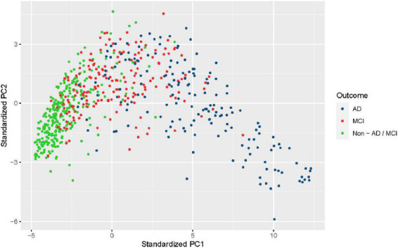
Visualization of the nursing dataset after dimension reduction with principal component analysis. Black dots represent patients diagnosed with Alzheimer’s disease (AD), red dots represent patients diagnosed with mild cognitive impairment (MCI), and green dots represent patients from neither class (non-AD/MCI).
For validation purposes, we collected data with the same cognitive status and non-imaging features from four communities across 12 counties in Zhejiang province. A multi-stage stratified random cluster sampling method was adopted to select the communities. We first divided 12 counties into four groups based on economic levels, then systematically selected one district from each of these four groups, and finally randomly chose one community from each district. The same inclusion/exclusion criteria and data processing progress as for the nursing dataset were applied (Figure 1). The final community dataset contains 1,100 cases, of which 59 (5.4%) were diagnosed with AD, 118 (10.7%) with MCI, and 923 (83.9%) with non-AD/MCI.
For the collection of the nursing and community data, ethics approval was obtained from the Ethics Committee of Zhejiang Hospital and informed consents were signed by participants.
Machine learning methods
Logistic regression
The logistic regression (Hosmer et al., 2013) is a classical machine learning method widely used in medical research. It performs well if there is a linear relationship between the features and logit of the outcome. Due to the simplicity of the design, inferences regarding the contribution of each feature in predicting the outcome can be easily drawn from the model. We used this simple but powerful classification model as a benchmark: the included machine learning models should have at least as good predictive performance as the logistic model.
Support vector machines
The SVM (Vapnik, 2013), a state-of-the-art machine learning algorithm, is a generalization of linear decision boundaries for classification. It has successful applications in a variety of medical classification tasks, e.g., diagnosing heart valve diseases (Comak et al., 2007), breast cancer (Akay, 2009), diabetes (Yu et al., 2010), etc. Using a kernel function, SVM can transform the data into a higher-dimensional space and construct a linear boundary in the new space while generating a non-linear boundary in the original space. In this study, we tried four different SVM models SVM_l, SVM_r, SVM_s, and SVM_p, which correspond to models obtained by using linear, radial basis, sigmoid, and polynomial kernel functions, respectively.
Neural networks
Neural networks are non-linear machine learning models with computing systems inspired by how the human brain processes information. They have been widely applied in image analysis, biochemical analysis, drug design, diagnostic systems, and other branches of human medicine (Amato et al., 2013). Despite the low interpretability, neural networks are very flexible and quite effective in purely predictive settings thanks to the model-free design. In this study, we used a feedforward neural network with a single layer of hidden neurons and L1 weight regularization, which can be thought of as a non-linear generalization of linear logistic regression. The single-layer design and weight regularization can constrain the complexity of the model and prevent it from overfitting.
Random forests
Random forests use de-correlated tree predictors to build powerful classification models (Breiman, 2001). By combining predictions from a large collection of individual decision trees, random forests outperform the individual tree predictor and produce more accurate predictions. Being easy to understand and effective to use, random forests have many applications in the medical field, such as predicting Alzheimer’s and other diseases (Khalilia et al., 2011; Gray et al., 2013; Kane et al., 2014). In the random forest, a small number of trees will lead to poor performance of the model while a large number will not cause the model to overfit (Hastie et al., 2001). Therefore, we used a large number of trees, 500 in this study, to build the random forest model. In the model training process, we also assessed the importance of each feature by computing the mean decrease in Gini Index (Louppe et al., 2013).
XGBoosting
Boosting uses a combination of many “weak” classifiers to generate an ultimate strong classifier (Hastie et al., 2001). Though less popular than SVMs and random forests, boosting can provide outstanding prediction performance (Zhang et al., 2017). One popular boosting algorithm is gradient boosted decision trees (GBDT) (Friedman, 2002), which use the decision tree as the weak learner and use the gradient descent algorithm to minimize the loss function of the model. In this paper, we implemented XGBoost (short for “Extreme Gradient Boosting”), one of the most efficient implementations of GBDT (Chen and Guestrin, 2016). Compared to GBDT, XGBoost achieves better performance by introducing the regularization term in the loss function (the model is trained by minimizing the loss function) and using a second-order Taylor approximation for the loss function.
The least absolute shrinkage and selection operator
To better understand the relationship between features and outcome variables, we employed the least absolute shrinkage and selection operator (LASSO) (Tibshirani, 1996), which allows automatic feature selection by adding an L1 regularization term to force coefficients of some features to be equal to zero. LASSO is a popular and arguably the most effective method for selecting features in a linear model (Hastie et al., 2017). It is especially useful when there is a need to analyze a large number of features. We implemented LASSO as a prediction model for AD/MCI. And we investigated the contribution of features to the outcome prediction by examining the coefficient paths of the model.
Best subset
Best subset selection is another approach to finding the most relevant features to predict the outcome of interest. By definition, it requires evaluating possible subsets of the collection of all features according to some criteria. Although this approach has unmatched advantages in terms of interpretability, it is computationally demanding when the number of features is large and is computationally infeasible when cross-validation is used to evaluate subsets. In this study, we used a two-step search strategy to approximate the optimal result of best subset selection and reduce the computational requirement: (1) for each S = 1,2,…,P, find the “best” S out of P features, where the best features here refer to the ones that can maximize the likelihood function of the logistic regression model (achieved by the “BeSS.ONE” function in the BeSS R package; Wen et al., 2017), (2) find the best number of S (achieved by regarding S as a parameter and tuning it with double CV).
Evaluation metrics and validation methods
We performed both internal and external validation for all proposed machine learning models. The performance of all models was then assessed and compared according to sensitivity (recall), specificity, accuracy, area under the receiver operating characteristic curve (AUROC), precision, F1-score, and area under the precision-recall curve (AUPRC). Note that AUROC summarizes the trade-off between sensitivity and specificity while the F1-score (harmonic mean of the precision and recall) and AUPRC summarize the trade-off between sensitivity and precision.
We trained and internally evaluated our proposed machine learning models on the nursing dataset. The nursing dataset (350 cases) was relatively small compared to the 70 features and complex machine learning models we selected. Splitting the dataset into training, validation, and test sets allows parameter tuning. However, this method does not yield reliable estimates because of the small test set. On the other hand, the traditional k-fold CV can lead to over-optimistic estimates of the model’s performance (Varma and Simon, 2006). Therefore, we considered a novel double CV that can take care of both model evaluation and parameter tuning (Krstajic et al., 2014). To perform the double CV, we divided the nursing dataset into 10 folds and performed the following for each model. (1) Left one fold for validation. (2) On the remaining 9 folds, performed a 10-fold CV to tune the parameters so that the optimal parameters maximized the average AUROC. (3) Used the optimal parameters to refit the model on the 9-folds. (4) Computed evaluation metrics for the model fitted in step (3) on the held-out fold in step (1). (5) Repeated steps (1)–(4) 10 times across the 10 folds of the nursing dataset to obtain the 10 sets of evaluation metrics and optimal parameters. The performance of each model evaluated internally on the nursing dataset was then represented by the average of 10 sets of evaluation metrics, i.e., the double CV metrics. The process of performing double CV is illustrated in Figure 3.
FIGURE 3.

Flowchart of the double cross-validation.
After internal validation, we performed an external validation for the models. The medians of 10 sets of optimal parameters from the double CV were used to train the final models on the whole nursing dataset. Then the evaluation metrics of each final model were computed on the community dataset.
Parameter optimization
In the inner loop of double CV, different parameter tuning methods were applied to different models. Logistic regression has no parameters to be tuned. Grid search was used in double CV to fine-tune the parameters in the four SVM models, neural network, random forest, LASSO, and best subset model. For the last two models, tuning parameters (L1 regularization parameter in LASSO and number of features “S” in the best subset) is effectively equivalent to performing feature selection. The XGBoost model contains many important parameters (e.g., learning rate, maximum depth of a tree, number of trees, etc.) and requires extensive tuning to reach the desired performance. To address this, we used the Gaussian process upper confidence bound (GP-UCB) algorithm (Srinivas et al., 2009) in the double CV to tune the parameters. GP-UCB is a popular Bayesian optimization algorithm that chooses parameters by controlling the exploration-exploitation tradeoffs.
Software
All statistical analyses were done in R (R version 3.6.2) using the following libraries: e1071, randomForest, nnet, NeuralNetTools, xgboost, rBayesianOptimization, glmnet, BeSS, ROCR, cutpointr, ggplot2, and their respective dependencies. The online screening tool was employed by using R Shiny.
Results
Models’ evaluation and comparison
We have applied a number of different machine learning algorithms to build prediction models for detecting AD/MCI. It is of interest to compare these methods and determine which one performed best.
Table 1 compares demographic characteristics of age, sex, education, and summary scores of cognitive tests across the normal, MCI, and AD groups. Table 2 reports the classification performance of each model evaluated internally by the double CV on the nursing dataset. The averages of the 10 values of sensitivity, specificity, accuracy, and AUROC in the outer loop of double CV were provided. It can be seen that the SVM_r model had the best sensitivity while the SVM_p had the best specificity. The SVM_p and LASSO had the best accuracy performance. The Neural network (Figure 4) achieved the best AUROC, followed by XGBoost and SVM_p.
TABLE 1.
Demographic characteristics of age, sex, education, and summary scores of cognitive tests across the normal, MCI, and AD groups.
| Nursing dataset |
Community dataset |
|||||||
| AD | MCI | Non-AD/MCI | Overall | AD | MCI | Non-AD/MCI | Overall | |
| (N = 168) | (N = 182) | (N = 304) | (N = 654) | (N = 59) | (N = 118) | (N = 923) | (N = 1,100) | |
| Sex | ||||||||
| Male | 52 (31.0%) | 63 (34.6%) | 114 (37.5%) | 229 (35.0%) | 30 (50.8%) | 48 (40.7%) | 448 (48.5%) | 526 (47.8%) |
| Female | 116 (69.0%) | 119 (65.4%) | 190 (62.5%) | 425 (65.0%) | 29 (49.2%) | 70 (59.3%) | 475 (51.5%) | 574 (52.2%) |
| Age (SD) | 85 (± 6.4) | 85 (± 5.6) | 82 (± 6.4) | 84 (± 6.3) | 80 (± 5.4) | 79 (± 5.7) | 75 (± 6.2) | 76 (± 6.3) |
| Education (SD) | 2.3 (± 1.3) | 2.7 (± 1.3) | 3.4 (± 1.4) | 2.9 (± 1.4) | 2.4 (± 1.2) | 2.9 (± 1.1) | 3.4 (± 1.2) | 3.3 (± 1.2) |
| Summary score of mini-cog test (SD) | 1.0 (± 1.1) | 2.1 (± 1.2) | 3.2 (± 0.88) | 2.3 (± 1.4) | 2.1 (± 1.2) | 2.6 (± 1.2) | 3.6 (± 0.69) | 3.4 (± 0.90) |
| Summary score of clock drawing test (SD) | 0.98 (± 1.4) | 2.4 (± 1.8) | 4.2 (± 1.3) | 2.9 (± 2.0) | 3.1 (± 1.6) | 3.9 (± 1.3) | 4.7 (± 0.70) | 4.6 (± 0.95) |
| Summary score of mini-mental state exam (SD) | 13 (± 6.6) | 22 (± 4.3) | 27 (± 2.6) | 22 (± 7.2) | 21 (± 4.7) | 24 (± 3.8) | 28 (± 2.2) | 28 (± 3.2) |
| Summary score of AD8 screening (SD) | 4.3 (± 2.6) | 2.1 (± 1.8) | 0.80 (± 1.1) | 2.1 (± 2.3) | 4.3 (± 2.2) | 3.8 (± 2.0) | 1.7 (± 1.1) | 2.0 (± 1.5) |
TABLE 2.
Classification performance of each model evaluated internally by the double CV on the nursing dataset.
| Method | Sensitivity | Specitivity | Accuracy | AUROC |
| Logistic regression | 0.8229 | 0.8289 | 0.8256 | 0.9068 |
| SVM_l | 0.8143 | 0.8453 | 0.8287 | 0.9127 |
| SVM_r | 0.8600 | 0.8455 | 0.8532 | 0.9287 |
| SVM_s | 0.8200 | 0.8976 | 0.8562 | 0.9374 |
| SVM_p | 0.8343 | 0.8947 | 0.8624 | 0.9378 |
| Neural network | 0.8429 | 0.8751 | 0.8578 | 0.9435 |
| Random forest | 0.8314 | 0.8618 | 0.8455 | 0.9340 |
| XGBoost | 0.8457 | 0.8552 | 0.8501 | 0.9398 |
| LASSO | 0.8400 | 0.8882 | 0.8624 | 0.9341 |
| Best subset | 0.8371 | 0.8553 | 0.8456 | 0.9141 |
FIGURE 4.

The final neural network model. Weights are color-coded by sign (blue+, gray−) and thickness is in proportion to magnitude. Input features include sex, age, Mini-Cog test (c1–c2), Clock Drawing test (d1–d5), Mini-Mental State exam (e11–e15, e21–e25, e31–e33, e41–e45, e51–e53, e61–e62, e7, e8, e91–e93, e10, e16), AD8 screening (f1–f8), education (h1), occupation (h22–h29), marital status (h32–h35, h37), past medical history (h61–66), number of medications (h8), smoking (h9), and drinking (h10).
Table 3 reports the classification performance of each model evaluated externally on the community dataset. Compared to the nursing dataset, the community data were collected at households and were based on a population with a low risk of AD/MCI. The observed outcomes were quite unbalanced between the two classes (16.1% AD/MCI vs. 83.9% normal). Therefore, in addition to sensitivity, specificity, accuracy, and AUROC, we recorded the metrics of precision, F1-score, and AUPRC as these metrics are especially useful for the unbalanced data. From Table 3, we can see that the SVM_r and SVM_p have the best accuracy. SVM_l, SVM_p, and random forest models are the top three models in terms of AUROC (> 0.92). The SVM_r and SVM_p models had the highest F1-scores while logistic regression, XGBoost, and best subset models had poor F1-scores. The AUPRC values of SVM models, neural network, and random forest were relatively high, while those of the remaining models were relatively low.
TABLE 3.
Classification performance of each model evaluated externally on the community dataset.
| Method | Sensitivity | Specitivity | Accuracy | AUROC | Precision | F1-score | AUPRC |
| Logistic regression | 0.6215 | 0.8895 | 0.8464 | 0.8435 | 0.5189 | 0.5656 | 0.5199 |
| SVM_l | 0.5763 | 0.9458 | 0.8864 | 0.9282 | 0.6711 | 0.6201 | 0.6652 |
| SVM_r | 0.6102 | 0.9404 | 0.8873 | 0.9137 | 0.6626 | 0.6353 | 0.6395 |
| SVM_s | 0.5650 | 0.9437 | 0.8827 | 0.9177 | 0.6579 | 0.6079 | 0.6560 |
| SVM_p | 0.6045 | 0.9415 | 0.8873 | 0.9213 | 0.6646 | 0.6331 | 0.6549 |
| Neural network | 0.5876 | 0.9426 | 0.8855 | 0.9139 | 0.6624 | 0.6228 | 0.6513 |
| Random forest | 0.5706 | 0.9437 | 0.8836 | 0.9259 | 0.6601 | 0.6121 | 0.6623 |
| XGBoost | 0.5424 | 0.9415 | 0.8773 | 0.9006 | 0.6400 | 0.5872 | 0.6323 |
| LASSO | 0.5932 | 0.9393 | 0.8836 | 0.9023 | 0.6522 | 0.6213 | 0.6284 |
| Best subset | 0.4859 | 0.9274 | 0.8564 | 0.8483 | 0.5621 | 0.5212 | 0.5432 |
Though, according to Tables 2, 3, no model appears to be superior to all other models by all evaluation metrics, we can find some clues based on the accuracy and AUROC. The accuracy is the most common and intuitive metric to compare models’ performance. SVM_p and LASSO have the best accuracy in the internal validation (balanced data) while SVM_r and SVM_p have the best accuracy in the external validation (imbalanced data). According to this metric, the SVM and LASSO models seem to be the best models. However, we must note that accuracies have flaws in comparing models’ overall performance. First, the metric is limited to a single decision threshold (0.5 in this study), with which the model’s prediction probability is compared to determine whether the outcome prediction is positive or negative. Second, the metric cannot be used to compare models that are built upon datasets with different outcome distributions. Third, the metric can be misleading on classification problems with a skewed class distribution. For example, the accuracy on a dataset with 10% positive cases can be at least 90% accurate.
Compared to the accuracy, AUROC is a more robust and informative evaluation metric as it summarizes the sensitivity and specificity across different decision thresholds and can be used to compare models on different (possibly skewed) outcome distributions. On the nursing dataset, the neural network, Xgboost, SVM_p have the highest AUROC values (Figure 5A). However, the neural network and Xgboost have a low AUROC on the community dataset (Figure 5B). On the community dataset, the SVM_l, random forest, and SVM_p were the top models in terms of AUROC, while the first two models had less performance than the third model on the nursing dataset. It can be seen that SVM_p is the only one performing well on both the nursing (balanced) and the community (unbalanced) datasets.
FIGURE 5.

ROC and PRC curves for the machine learning models for detecting dementia. (A) Mean ROC curves for the models on the nursing datasets. Each curve represents the mean ROC curve from the outer loop of the double cross validation. (B) ROC curves for the models on the community data. (C) PRC curves for the models on the community data.
While ROC can be used for skewed outcome distributions, it may mask poor performance under unbalanced data (Jeni et al., 2013). F1 score and AUPRC, two metrics based on precision, are useful for the unbalanced setting since precision is an informative measure under imbalanced data (Saito and Rehmsmeier, 2015). We examined F1-score and AUPRC on the community dataset to rule out underperforming models on these two metrics. It can be seen that SVM_p has relatively high scores on these two measures (Figure 5C), which again confirms that SVM_p is robust on the unbalanced data. Through the above analysis, we concluded that overall SVM_p is the best AD/MCI detection model. We had implemented SVM_p online for patients and healthcare professionals to access (R Shiny).1
In terms of AUROC, our SVM_p is one of the best-performing models in predicting dementia to date (Hou et al., 2019). While most published models relied on a small number of features and few reported (proper) validation results (Pellegrini et al., 2018; Hou et al., 2019), our models took advantage of 70 features and went through both internal (double cross) validation and external validation.
Therefore, our study made maximum use of the information from available features while ensuring the reliability and repeatability of the results.
Features’ contribution
Some of the machine learning models we built enabled us to see the contribution of the features for predicting AD/MCI. We studied the relative importance of features by the tree-based random forests and XGBoost models and further investigated the role of the important features by the Lasso model and the best subset model.
In the random forest model, the Gini index is used to decide which feature to split at each node within each component tree classifier. Each split of a node results in a decrease in Gini where the magnitude of the decrease indicates the discriminatory power of the split. For each feature, the decrease in the Gini index is accumulated each time the feature is selected to split a node. Therefore, the average decrease over all component tree classifiers for each feature can be used to represent the contribution of this feature to the prediction and thus serve as a measure of importance. A greater mean decrease means higher importance. Based on information gain, a measure similar to the mean decrease in Gini, the XGBoost can also compute each feature’s contribution to the model using all the splits.
Supplementary Figure 1A presents the 20 most important features based on the final random forest model. It can be seen that the tests of counting down from 100 by 7 (e41-e45) and clocking drawing (d1-d5) are of most importance for predicting outcome. Mini-Cog test (c1-c2), time orientation test (e11-e15), and age have a lower level of importance. Of less importance is the test of copy drawing (e16), the test of repeating phrase (e7), the test of repeating previous items (e51-e53), medications (h8), and others. The feature importance rankings given by the XGBoost model are similar to those given by the random forest (Supplementary Figure 1B), while the former highlights the importance of education (h1), and AD8 Dementia Screening (f1-f8), and the test of saying a complete sentence (e10).
To understand the specific impact of important features, we also studied the features selected by the LASSO and best subset model and analyzed the signs of the features’ coefficients. In the final LASSO model, the L1 regularization shrunk the coefficients of less important features to zero. There were 35 features considered by LASSO to be relevant to outcome prediction (Supplementary Figures 2A,B). In contrast, the best subset model selected 19 features (Supplementary Figure 2C), almost all of which are included in the features selected by LASSO. These results show that many non-imaging features could help predict AD/MCI.
Specifically, 17 were selected by both LASSO and best subset. These features were most likely to be relevant to AD/MCI prediction, including age, Mini-Cog test (c2), clocking drawing test (d2, d5), time orientation test (e15), address orientation test (e23), the test of counting down from 100 by 7 (e43, e44), the test of repeating previous items (e51, e52), the test of repeating previous items (e7), the test of saying a complete sentence (e10), AD8 Dementia Screening (f6, f8), education (h1), “cadres staff” in the occupation (h24), and “married” in the marital status (h32). For these 17 features, LASSO and the best subset agreed on the signs of their coefficients. These signs allow us to further understand the influence of the features on predicting the disease. From Supplementary Figure 2B, it can be seen that the coefficients of all test-related features were negative, which is reasonable since passing the test indicates a lower likelihood of developing AD/MCI. “Married” (compared to “single”) in the marital status also suggests a lower risk. On the other hand, age, “handling complex personal financial matters” (f6) and “daily memory and thinking” (f8) in AD8 screening, education, and “cadres staff” (compared to “worker”) in the occupation (h24) have positive coefficients, suggesting that these features are risk indicators.
In the nursing dataset, if we only look at education without considering other features, then education is negatively associated with ADI/MCI (Figure 6A). But this relationship is reversed when other features are taken into account (Supplementary Figures 2B,C). These results of education echo the findings that the role of education can be controversial in predicting the risk of dementia (Caamaño-Isorna et al., 2006; Sharp and Gatz, 2011). Instead of being an independent risk factor, education could be a factor that protects against or delays the clinical manifestations of dementia. In other words, patients with a severe brain damage and a high educational level may present similar clinical symptoms of the disease as those with a less severe brain damage and a lower educational level. This view can also be confirmed by the results in Figure 6B where education is highly positively correlated with cognitive abilities (Mini-Cog, Clock Drawing, MMSE) and negatively correlated with cognitive problems (AD8 Screening features). Therefore, our model in fact suggests that a higher educational level may mean more severe brain damage if cognitive levels are equal.
FIGURE 6.

The role of education in predicting dementia. (A) The marginal distribution of the levels of education on the nursing dataset. (B) The correlation coefficients between education and other features on the nursing dataset.
Discussion
We created and validated our AD/MCI diagnostic tool using extensive data collected from the nursing home and the communities. These data are readily available and closely related to clinical diagnosis, which makes our model highly applicable. The applicability of our tool is further enhanced by its online deployment. Patients and clinicians who do not understand machine learning algorithms can easily input the collected non-imaging features into our tool to obtain timely predictive results. Compared to the traditional clinical screening of scales, our approach simplifies the data collection task and quickly performs high-quality analysis, thus greatly improving the diagnostic efficiency of clinicians. In addition, our approach does not involve any risk of complications associated with invasive biopsies, nor rely on equipment and operators for medical imaging systems. These merits make our approach almost free of test costs or risk of use, therefore avoiding economic or health impacts on patients and their families. We believe it has great potential applications, especially in small cities and rural areas.
Conclusion
Automated diagnostic tools have become crucial in the diagnosis of dementia. Although neuro-images have been heavily used in recently developed tools, traditional non-imaging features can effectively diagnose dementia and conveniently incorporate clinical practice. We used a large number of non-imaging features and machine learning to create a highly performing dementia diagnostic tool. Our work leverages the predictive potential of non-imaging features and significantly lowers the barriers for using the diagnostic tool. We believe this study will have a direct impact on physicians’ diagnostic practice and patients’ self-screening.
Data availability statement
The original contributions presented in this study are included in the article/Supplementary material, further inquiries can be directed to the corresponding authors.
Author contributions
XX, HW, JY, and GM conceived and designed the study. SX, YJ, XJ, and SQ collected the data. HW, XX, LS, and QC performed data analysis. HW, XX, WX, and ZZ made the figures. HW and XX wrote the manuscript. All authors reviewed, approved the final version of the manuscript, and agreed to be accountable for the content of the work.
Abbreviations
- MCI
mild cognitive impairment
- Aβ
amyloid beta
- VaD
vascular dementia
- FTD
frontotemporal dementia
- DLB
dementia with Lewy bodies
- SVM
support vector machine
- XGBoost
extreme gradient boosting
- LASSO
least absolute shrinkage and selection operator
- ANN
artificial neural networks
- CV
cross-validation
- CDT
clock drawing test
- MMSE
Mini-Mental State Exam
- CDR
clinical dementia rating
- GBDT
gradient boosted decision trees
- AUROC
area under the receiver operating characteristic curve
- AUPRC
area under the precision-recall curve
- GP-UCB
Gaussian process upper confidence bound.
Footnotes
Funding
This study was supported by funds from the Zhejiang Province Basic Public Welfare Research Project (LGF21H250002), Chinese Traditional Medicine Science and Technology Projects of Zhejiang Province (2021ZB002 and 2022ZB002), and Health Bureau of Zhejiang Province (2019RC092 and 2020KY394).
Conflict of interest
The authors declare that the research was conducted in the absence of any commercial or financial relationships that could be construed as a potential conflict of interest.
Publisher’s note
All claims expressed in this article are solely those of the authors and do not necessarily represent those of their affiliated organizations, or those of the publisher, the editors and the reviewers. Any product that may be evaluated in this article, or claim that may be made by its manufacturer, is not guaranteed or endorsed by the publisher.
Supplementary material
The Supplementary Material for this article can be found online at: https://www.frontiersin.org/articles/10.3389/fnagi.2022.945274/full#supplementary-material
References
- Aderghal K., Khvostikov A., Krylov A., Benois-Pineau J., Afdel K., Catheline G. (2018). “Classification of Alzheimer disease on imaging modalities with deep CNNs using cross-modal transfer learning,” in 2018 IEEE 31st International Symposium on Computer-Based Medical Systems (CBMS), (New York, NY: IEEE; ), 345–350. 10.1109/CBMS.2018.00067 [DOI] [Google Scholar]
- Akay M. F. (2009). Support vector machines combined with feature selection for breast cancer diagnosis. Expert Syst. Appl. 36 3240–3247. 10.1016/j.eswa.2008.01.009 [DOI] [Google Scholar]
- Albert M. S., DeKosky S. T., Dickson D., Dubois B., Feldman H. H., Fox N. C., et al. (2011). The diagnosis of mild cognitive impairment due to Alzheimer’s disease: Recommendations from the National Institute on Aging-Alzheimer’s Association workgroups on diagnostic guidelines for Alzheimer’s disease. Alzheimers Dement. 7 270–279. 10.1016/j.jalz.2011.03.008 [DOI] [PMC free article] [PubMed] [Google Scholar]
- Amato F., López A., Peña-Méndez E. M., Vaňhara P., Hampl A., Havel J. (2013). Artificial Neural Networks in Medical Diagnosis. Amsterdam: Elsevier. 10.2478/v10136-012-0031-x [DOI] [Google Scholar]
- Azevedo L., Calandri I. L., Slachevsky A., Graviotto H. G., Vieira M. C. S., Andrade C. B., et al. (2021). Impact of Social Isolation on People with Dementia and Their Family Caregivers. J. Alzheimers Dis. 81 607–617. 10.3233/JAD-201580 [DOI] [PMC free article] [PubMed] [Google Scholar]
- Barthel H., Schroeter M. L., Hoffmann K. T., Sabri O. (2015). PET/MR in dementia and other neurodegenerative diseases. Semin. Nucl. Med. 45 224–233. 10.1053/j.semnuclmed.2014.12.003 [DOI] [PubMed] [Google Scholar]
- Bissig D., DeCarli C. S. (2019). Global & Community Health: Brief in-hospital cognitive screening anticipates complex admissions and may detect dementia. Neurology 92 631–634. 10.1212/WNL.0000000000007176 [DOI] [PMC free article] [PubMed] [Google Scholar]
- Breiman L. (2001). Random forests. Mach. Learn. 45 5–32. 10.1023/A:1010933404324 [DOI] [Google Scholar]
- Bruun M., Rhodius-Meester H. F. M., Koikkalainen J., Baroni M., Gjerum L., Lemstra A. W., et al. (2018). Evaluating combinations of diagnostic tests to discriminate different dementia types. Alzheimers Dement. 10 509–518. 10.1016/j.dadm.2018.07.003 [DOI] [PMC free article] [PubMed] [Google Scholar]
- Caamaño-Isorna F., Corral M., Montes-Martínez A., Takkouche B. (2006). Education and dementia: A meta-analytic study. Neuroepidemiology 26 226–232. 10.1159/000093378 [DOI] [PubMed] [Google Scholar]
- Cai H., Sha X., Han X., Wei S., Hu B. (2016). “Pervasive EEG diagnosis of depression using Deep Belief Network with three-electrodes EEG collector,” in 2016 IEEE International Conference on Bioinformatics and Biomedicine (BIBM), (Amsterdam: IEEE; ), 1239–1246. [Google Scholar]
- Chen T., Guestrin C. (2016). “Xgboost: A scalable tree boosting system,” in Proceedings of the 22nd ACM Sigkdd International Conference on Knowledge Discovery and Data Mining, (New York, NY: Association for Computing Machinery; ). 785–794. 10.1145/2939672.2939785 [DOI] [Google Scholar]
- Comak E., Arslan A., Turkoglu I. (2007). A decision support system based on support vector machines for diagnosis of the heart valve diseases. Comput. Biol. Med. 37 21–27. 10.1016/j.compbiomed.2005.11.002 [DOI] [PubMed] [Google Scholar]
- Cui R., Liu M., Alzheimer’s Disease Neuroimaging I. (2019). RNN-based longitudinal analysis for diagnosis of Alzheimer’s disease. Comput. Med. Imaging Graph. 73 1–10. 10.1016/j.compmedimag.2019.01.005 [DOI] [PubMed] [Google Scholar]
- Ding Y., Sohn J. H., Kawczynski M. G., Trivedi H., Harnish R., Jenkins N. W., et al. (2019). A Deep Learning Model to Predict a Diagnosis of Alzheimer Disease by Using (18)F-FDG PET of the Brain. Radiology 290 456–464. 10.1148/radiol.2018180958 [DOI] [PMC free article] [PubMed] [Google Scholar]
- Dolph C. V., Alam M., Shboul Z., Samad M. D., Iftekharuddin K. M. (2017). “Deep learning of texture and structural features for multiclass Alzheimer’s disease classification,” in 2017 International Joint Conference on Neural Networks (IJCNN), (Amsterdam: IEEE; ), 2259–2266. 10.1109/IJCNN.2017.7966129 [DOI] [Google Scholar]
- Feldman H., Ganguli M., Hampel H., Scheltens P., Tierney M. C., Whitehouse P., et al. (2006). International Psychogeriatric Association Expert Conference on mild cognitive impairment. Mild cognitive impairment. Lancet 367 1262–1270. 10.1016/S0140-6736(06)68542-5 [DOI] [PubMed] [Google Scholar]
- Friedman J. H. (2002). Stochastic gradient boosting. Comput. Stat. Data Anal. 38 367–378. 10.1016/S0167-9473(01)00065-2 [DOI] [Google Scholar]
- Geldmacher D. S., Whitehouse P. J. (1996). Evaluation of dementia. N. Engl. J. Med. 335 330–336. 10.1056/NEJM199608013350507 [DOI] [PubMed] [Google Scholar]
- Gray K. R., Aljabar P., Heckemann R. A., Hammers A., Rueckert D., Initiative A. S. D. N. (2013). Random forest-based similarity measures for multi-modal classification of Alzheimer’s disease. NeuroImage 65 167–175. 10.1016/j.neuroimage.2012.09.065 [DOI] [PMC free article] [PubMed] [Google Scholar]
- Grundman M., Petersen R. C., Ferris S. H., Thomas R. G., Aisen P. S., Bennett D. A., et al. (2004). Mild cognitive impairment can be distinguished from Alzheimer disease and normal aging for clinical trials. Arch. Neurol. 61 59–66. 10.1001/archneur.61.1.59 [DOI] [PubMed] [Google Scholar]
- Hastie T., Tibshirani R., Friedman J. (2001). The Elements of Statistical Learning. Springer Series in Statistics. Germany: Springer. 10.1007/978-0-387-21606-5 [DOI] [Google Scholar]
- Hastie T., Tibshirani R., Tibshirani R. J. (2017). Extended comparisons of best subset selection, forward stepwise selection, and the lasso. arXiv. [Preprint]. [Google Scholar]
- Hon M., Khan N. M. (2017). “Towards Alzheimer’s disease classification through transfer learning,” in 2017 IEEE International Conference on Bioinformatics and Biomedicine (BIBM), (Amsterdam: IEEE; ), 1166–1169. 10.1109/BIBM.2017.8217822 [DOI] [Google Scholar]
- Hosmer D. W., Jr., Lemeshow S., Sturdivant R. X. (2013). Applied Logistic Regression. Hoboken: John Wiley & Sons. 10.1002/9781118548387 [DOI] [Google Scholar]
- Hosseini-Asl E., Keynton R., El-Baz A. (2016). “Alzheimer’s disease diagnostics by adaptation of 3D convolutional network,” in 2016 IEEE International Conference on Image Processing (ICIP), (Amsterdam: IEEE; ), 126–130. 10.1109/ICIP.2016.7532332 [DOI] [Google Scholar]
- Hou X.-H., Feng L., Zhang C., Cao X.-P., Tan L., Yu J.-T. (2019). Models for predicting risk of dementia: A systematic review. J. Neurol. Neurosurg. Psychiatry 90 373–379. 10.1136/jnnp-2018-318212 [DOI] [PubMed] [Google Scholar]
- Ishii K. (2014). PET approaches for diagnosis of dementia. AJNR Am. J. Neuroradiol. 35 2030–2038. 10.3174/ajnr.A3695 [DOI] [PMC free article] [PubMed] [Google Scholar]
- Islam J., Zhang Y. (2017). “A novel deep learning based multi-class classification method for Alzheimer’s disease detection using brain MRI data,” in International Conference on Brain Informatics, (Germany: Springer; ), 213–222. 10.1007/978-3-319-70772-3_20 [DOI] [Google Scholar]
- Janelidze S., Mattsson N., Palmqvist S., Smith R., Beach T. G., Serrano G. E., et al. (2020). Plasma P-tau181 in Alzheimer’s disease: Relationship to other biomarkers, differential diagnosis, neuropathology and longitudinal progression to Alzheimer’s dementia. Nat. Med. 26 379–386. 10.1038/s41591-020-0755-1 [DOI] [PubMed] [Google Scholar]
- Jeni L. A., Cohn J. F., De La Torre F. (2013). “Facing imbalanced data–recommendations for the use of performance metrics,” in 2013 Humaine Association Conference on Affective Computing and Intelligent Interaction, (Amsterdam: IEEE; ), 245–251. 10.1109/ACII.2013.47 [DOI] [PMC free article] [PubMed] [Google Scholar]
- Jo T., Nho K., Saykin A. J. (2019). Deep Learning in Alzheimer’s Disease: Diagnostic Classification and Prognostic Prediction Using Neuroimaging Data. Front. Aging Neurosci. 11:220. 10.3389/fnagi.2019.00220 [DOI] [PMC free article] [PubMed] [Google Scholar]
- Josephson S. A., Papanastassiou A. M., Berger M. S., Barbaro N. M., McDermott M. W., Hilton J. F., et al. (2007). The diagnostic utility of brain biopsy procedures in patients with rapidly deteriorating neurological conditions or dementia. J. Neurosurg. 106 72–75. 10.3171/jns.2007.106.1.72 [DOI] [PubMed] [Google Scholar]
- Kane M. J., Price N., Scotch M., Rabinowitz P. (2014). Comparison of ARIMA and Random Forest time series models for prediction of avian influenza H5N1 outbreaks. BMC Bioinformatics 15:276. 10.1186/1471-2105-15-276 [DOI] [PMC free article] [PubMed] [Google Scholar]
- Khalilia M., Chakraborty S., Popescu M. (2011). Predicting disease risks from highly imbalanced data using random forest. BMC Med. Inform. Decis. Mak. 11:51. 10.1186/1472-6947-11-51 [DOI] [PMC free article] [PubMed] [Google Scholar]
- Khvostikov A., Aderghal K., Benois-Pineau J., Krylov A., Catheline G. (2018). 3D CNN-based classification using sMRI and MD-DTI images for Alzheimer disease studies. arXiv [Preprint]. [Google Scholar]
- Krstajic D., Buturovic L. J., Leahy D. E., Thomas S. (2014). Cross-validation pitfalls when selecting and assessing regression and classification models. J. Cheminform. 6:10. 10.1186/1758-2946-6-10 [DOI] [PMC free article] [PubMed] [Google Scholar]
- Lee G., Nho K., Kang B., Sohn K. A., Kim D., for Alzheimer’s Disease Neuroimaging I. (2019). Predicting Alzheimer’s disease progression using multi-modal deep learning approach. Sci. Rep. 9:1952. 10.1038/s41598-018-37769-z [DOI] [PMC free article] [PubMed] [Google Scholar]
- Leinonen V., Koivisto A. M., Savolainen S., Rummukainen J., Tamminen J. N., Tillgren T., et al. (2010). Amyloid and tau proteins in cortical brain biopsy and Alzheimer’s disease. Ann. Neurol. 68 446–453. 10.1002/ana.22100 [DOI] [PubMed] [Google Scholar]
- Long J. M., Holtzman D. M. (2019). Alzheimer Disease: An Update on Pathobiology and Treatment Strategies. Cell 179 312–339. 10.1016/j.cell.2019.09.001 [DOI] [PMC free article] [PubMed] [Google Scholar]
- Louppe G., Wehenkel L., Sutera A., Geurts P. (2013). Understanding variable importances in forests of randomized trees. Adv. Neural. Inf. Process. Syst. 26 431–439. [Google Scholar]
- Maroco J., Silva D., Rodrigues A., Guerreiro M., Santana I., de Mendonça A. (2011). Data mining methods in the prediction of Dementia: A real-data comparison of the accuracy, sensitivity and specificity of linear discriminant analysis, logistic regression, neural networks, support vector machines, classification trees and random forests. BMC Res. Notes 4:299. 10.1186/1756-0500-4-299 [DOI] [PMC free article] [PubMed] [Google Scholar]
- McKhann G. M., Knopman D. S., Chertkow H., Hyman B. T., Jack C. R., Jr., Kawas C. H., et al. (2011). The diagnosis of dementia due to Alzheimer’s disease: Recommendations from the National Institute on Aging-Alzheimer’s Association workgroups on diagnostic guidelines for Alzheimer’s disease. Alzheimers Dement. 7 263–269. 10.1016/j.jalz.2011.03.005 [DOI] [PMC free article] [PubMed] [Google Scholar]
- Mitchell S. L., Teno J. M., Kiely D. K., Shaffer M. L., Jones R. N., Prigerson H. G., et al. (2009). The clinical course of advanced dementia. N. Engl. J. Med. 361 1529–1538. 10.1056/NEJMoa0902234 [DOI] [PMC free article] [PubMed] [Google Scholar]
- Mosconi L. (2013). Glucose metabolism in normal aging and Alzheimer’s disease: Methodological and physiological considerations for PET studies. Clin. Transl. Imaging 1:10. 10.1007/s40336-013-0026-y [DOI] [PMC free article] [PubMed] [Google Scholar]
- Pellegrini E., Ballerini L., Hernandez M., Chappell F. M., Gonzalez-Castro V., Anblagan D., et al. (2018). Machine learning of neuroimaging for assisted diagnosis of cognitive impairment and dementia: A systematic review. Alzheimers Dement. 10 519–535. 10.1016/j.dadm.2018.07.004 [DOI] [PMC free article] [PubMed] [Google Scholar]
- Petersen R. C., Smith G. E., Waring S. C., Ivnik R. J., Tangalos E. G., Kokmen E. (1999). Mild cognitive impairment: Clinical characterization and outcome. Arch. Neurol. 56 303–308. 10.1001/archneur.56.3.303 [DOI] [PubMed] [Google Scholar]
- Rabins P. V., Mace N. L., Lucas M. J. (1982). The impact of dementia on the family. JAMA 248 333–335. 10.1001/jama.1982.03330030039022 [DOI] [PubMed] [Google Scholar]
- Saito T., Rehmsmeier M. (2015). The precision-recall plot is more informative than the ROC plot when evaluating binary classifiers on imbalanced datasets. PLoS One 10:e0118432. 10.1371/journal.pone.0118432 [DOI] [PMC free article] [PubMed] [Google Scholar]
- Sarraf S., Tofighi G. (2016). Classification of alzheimer’s disease using fmri data and deep learning convolutional neural networks. arXiv [Preprint]. [Google Scholar]
- Selkoe D. J. (2019). Early network dysfunction in Alzheimer’s disease. Science 365 540–541. 10.1126/science.aay5188 [DOI] [PubMed] [Google Scholar]
- Shankle W. R., Mani S., Pazzani M. J., Smyth P. (1997). “Detecting very early stages of dementia from normal aging with machine learning methods,” in Conference on Artificial Intelligence in Medicine in Europe, (Berlin: Springer; ), 71–85. 10.1007/BFb0029438 [DOI] [Google Scholar]
- Sharp E. S., Gatz M. (2011). The relationship between education and dementia an updated systematic review. Alzheimer Dis. Assoc. Disord. 25:289. 10.1097/WAD.0b013e318211c83c [DOI] [PMC free article] [PubMed] [Google Scholar]
- Sheehan B. (2012). Assessment scales in dementia. Ther. Adv. Neurol. Disord. 5 349–358. 10.1177/1756285612455733 [DOI] [PMC free article] [PubMed] [Google Scholar]
- Shi B., Chen Y., Zhang P., Smith C. D., Liu J., Initiative A. S. D. N. (2017). Nonlinear feature transformation and deep fusion for Alzheimer’s Disease staging analysis. Pattern Recognize. 63 487–498. 10.1016/j.patcog.2016.09.032 [DOI] [Google Scholar]
- Shivamurthy V. K., Tahari A. K., Marcus C., Subramaniam R. M. (2015). Brain FDG PET and the diagnosis of dementia. AJR Am. J. Roentgenol. 204 W76–W85. 10.2214/AJR.13.12363 [DOI] [PubMed] [Google Scholar]
- Srinivas N., Krause A., Kakade S. M., Seeger M. (2009). Gaussian process optimization in the bandit setting: No regret and experimental design. Proceedings of the 27th International Conference on Machine Learning, Pennsylvania: University of Pennsylvania. 1015-1022 [Google Scholar]
- Tibshirani R. (1996). Regression shrinkage and selection via the lasso. J. R Stat. Soc. 58 267–288. 10.1111/j.2517-6161.1996.tb02080.x [DOI] [Google Scholar]
- Vapnik V. (2013). The Nature of Statistical Learning Theory. Germany: Springer science & business media. [Google Scholar]
- Varma S., Simon R. (2006). Bias in error estimation when using cross-validation for model selection. BMC Bioinformatics 7:91. 10.1186/1471-2105-7-91 [DOI] [PMC free article] [PubMed] [Google Scholar]
- Warren J. D., Schott J. M., Fox N. C., Thom M., Revesz T., Holton J. L., et al. (2005). Brain biopsy in dementia. Brain 128 2016–2025. 10.1093/brain/awh543 [DOI] [PubMed] [Google Scholar]
- Wen C., Zhang A., Quan S., Wang X. (2017). Bess: An r package for best subset selection in linear, logistic and CoxPH models. J. Stat. Softw. 94 1–24. 10.18637/jss.v094.i04 [DOI] [Google Scholar]
- Yu W., Liu T., Valdez R., Gwinn M., Khoury M. J. (2010). Application of support vector machine modeling for prediction of common diseases: The case of diabetes and pre-diabetes. BMC Med. Inform. Decis. Mak. 10:16. 10.1186/1472-6947-10-16 [DOI] [PMC free article] [PubMed] [Google Scholar]
- Zhang C., Liu C., Zhang X., Almpanidis G. (2017). An up-to-date comparison of state-of-the-art classification algorithms. Expert Syst. Appl. 82 128–150. 10.1016/j.eswa.2017.04.003 [DOI] [Google Scholar]
Associated Data
This section collects any data citations, data availability statements, or supplementary materials included in this article.
Supplementary Materials
Data Availability Statement
The original contributions presented in this study are included in the article/Supplementary material, further inquiries can be directed to the corresponding authors.