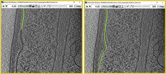
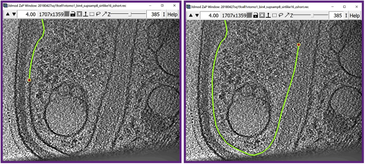
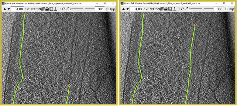
Summary
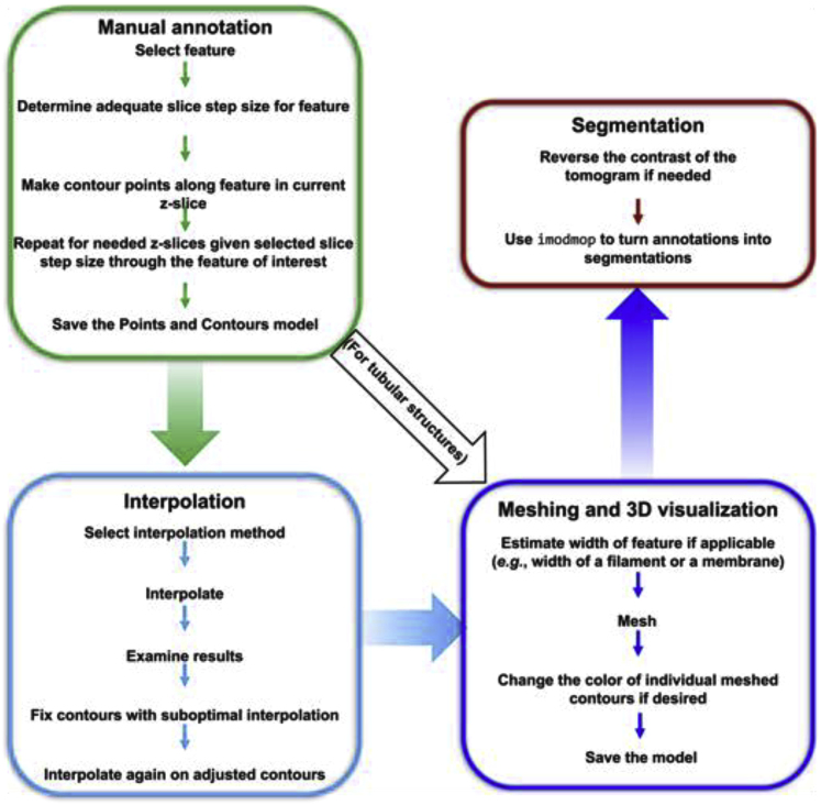
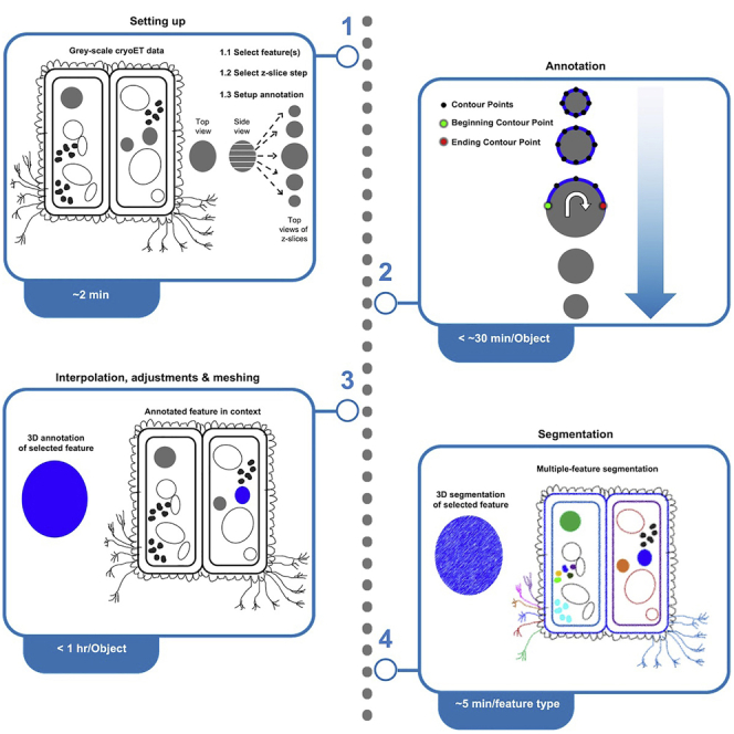
Annotation highlights and segmentation isolates features in cryogenic electron tomograms to improve visualization and quantification of features (for example, their size and abundance, and spatial relationships with other features), facilitating phenotypic structural analyses of cellular tomograms. Here, we present a manual annotation protocol using the open-source software IMOD and describe segmentation of three types of common cellular features: membranes, large globules, and filaments. IMOD’s interpolation function can improve the speed of manual annotation up to an order of magnitude.
Subject areas: Cell biology, Cell membrane, Structural biology, Cryo-EM, Evolutionary biology
Graphical abstract
Highlights
-
•
Interpolation between sparsely annotated slices speeds up manual annotation
-
•
Manual annotation differentiates between similar features in different contexts
-
•
Turning annotations into segmentations shows actual data instead of representations of it
Publisher’s note: Undertaking any experimental protocol requires adherence to local institutional guidelines for laboratory safety and ethics.
Annotation highlights and segmentation isolates features in cryogenic electron tomograms to improve visualization and quantification of features (for example, their size and abundance, and spatial relationships with other features), facilitating phenotypic structural analyses of cellular tomograms. Here, we present a manual annotation protocol using the open-source software IMOD and describe segmentation of three types of common cellular features: membranes, large globules, and filaments. IMOD’s interpolation function can improve the speed of manual annotation up to an order of magnitude.
Before you begin
This protocol exemplifies efficient manual annotation of various features in rectangular cell-like units (Dudek et al., 2021). However, we have successfully used it to annotate features in other types of cells and organelles, including patient-derived induced-pluripotent stem cells (iPSCs) differentiated into neurons (Wu et al., 2022). While manual annotation of features in cryo-electron tomography (cryo-ET) tomograms can suffer from bias and other caveats (Hecksel et al., 2016), algorithms for automated or semi-automated annotation often target specific types of features (Martinez-Sanchez et al., 2011) or can yield many false positives and false negatives, depending on data quality, alignment and reconstruction accuracy, or on the variability in user-defined negative and positive references for neural network based algorithms (Chen et al., 2017). Sometimes, challenging datasets such as cryo-ET tomograms of very thick samples (400–600 nm thick) may need extensive manual cleanup after automated or semi-automated annotation, making the process much less efficient. Also, current automated algorithms cannot easily distinguish between two morphologically similar yet distinct features; for example, membranes, vesicles, or small globules may functionally acquire different identities based largely on their relative context within the cell but may be otherwise chemically similar or identical and structurally indistinguishable at typical cryo-ET resolutions in the absence of averaging.
Here, we present a protocol for manual annotation using IMOD (Kremer et al., 1996), the most widely used software for electron microscopy (EM) tomographic reconstruction. We exemplify our manual annotation protocol using three different types of features in cryo-ET tomograms of enigmatic bacterial rectangular cell-like units with an unusual rectangular morphology, recently discovered among the microbiome of bottlenose dolphin mouths (Dudek et al., 2021). The selected features were lipid membranes, large globules, and filamentous structures, all of which are common among most cellular specimens. The reader should be able to successfully annotate various features in their own datasets following the instructions in this protocol.
Install IMOD
Timing: < 2 h
This section provides brief, general considerations for installing IMOD.
-
1.
Install IMOD.
Note: Installing this package on all of the three most popular operating systems (Linux, MacOSX, and Windows) should be relatively easy and we have noticed no relevant differences among them in terms of running IMOD programs. For the examples presented in this protocol, we used IMOD version 4.10.47 on a laptop running the Windows 10 operating system (OS). Full configuration should take ∼1–2 h or less even without any prior experience. Detailed instructions for installation and configuration are described in the IMOD User’s Guide online (see key resources table). A modest computer (including student laptops, for example), with ∼125 gigabytes (GB) of hard drive storage and ∼4 GB of RAM memory should be more than sufficient to complete manual annotations of cryo-ET tomograms of cellular specimens or other biological systems of interest of ∼1024 × 1024 × 300 voxels in size. In practice, a computer should have sufficient hard drive and RAM memory to store and open the tomograms, respectively. This will depend on the size of the tomograms, which can vary widely depending on their X, Y and Z dimensions and the datatype of these 3D images. The manual annotation and segmentation procedure described here does not exclusively apply to cryo-ET data and may be suitable for annotating tomograms reconstructed from tilt series collected with other imaging modalities, such as scanning electron microscopy (Wolf et al., 2014), or transmission electron microscopy of fixed/stained specimens at room temperature (Frank, 2013). For most cryo-ET applications, full floating point precision data type, binned-by-4 tomograms are typically no larger than a few of GBs.
Image processing
Timing: < 5 h
This section provides context for annotation and segmentation of cryo-ET tomograms and suggestions regarding image processing steps that may be useful before starting the annotation.
-
2.
Reconstruct the tomograms.
Note: Tilt series can be aligned and reconstructed into tomograms with various software packages, amply listed in comprehensive reviews (Fernandez, 2012; Galaz-Montoya and Ludtke, 2017). Some automated alignment and reconstruction methods targeting subsequent subtomogram averaging analyses at the sub-tilt series or per-particle level such as the latest pipeline in EMAN2 (Chen et al., 2019) may yield tomograms quickly processed in bulk (using the same parameters) with sufficient quality to identify large macromolecular complexes or “particles” within them, but may present more distortions and artifacts than careful fiducial-based or patch-tracking-based alignment of individual tomograms as done in IMOD. Indeed, many software packages for tomographic reconstruction can use IMOD-aligned tilt series but apply alternative reconstruction techniques to produce the final tomograms (Yan et al., 2019) (Deng et al., 2016) (Himes and Zhang, 2018) (Turoňová et al., 2017) (Tegunov and Cramer, 2019). While the protocol presented here can be applied to any IMOD-compatible 3D image with putative features to annotate irrespective of alignment or reconstruction software, for simplicity and to optimize quality that will in turn increase confidence during annotation, we recommend performing tilt series alignment with IMOD. The IMOD-aligned tilt series may then be reconstructed with any of the other software packages referenced above, which may increase contrast for some datasets while partially filling in the “missing wedge” artifact (Yan et al., 2019) (Deng et al., 2016), present in all limited-angle tomography experiments.
-
3.
Down sample the tomograms.
Note: The resolution of raw cryo-ET tomograms is relatively low due to challenges inherent in the specimen and the data collection methodology. Such challenges include the thickness of cryo-ET specimens (in the range of hundreds of nanometers) even after focused ion beam (FIB) milling (Marko et al., 2007) (indeed, some studies purposefully produce lamella at the thickness limit of the electron microscope’s penetration power to preserve more of the cellular context surrounding the features of interest (Wu et al., 2020)), the low-dose imaging conditions purposefully set to minimize radiation damage of the specimen from the electron beam during imaging, and the depth of focus through thick specimens (Jensen and Kornberg, 2000) (Galaz-Montoya et al., 2015), among others. Another challenge arises with the contrast transfer function (CTF) of the electron microscope that is particularly difficult to correct for in cryo-ET due to the defocus gradient arising from the tilting geometry during tilt series collection (Winkler and Taylor, 2003) (Fernández et al., 2006) (Galaz-Montoya et al., 2016). Thus, depending on the sampling size of the imaging data and the specific goals of a project, raw tomograms can often be downsampled (or “binned”) without loss of meaningful information for purposes of visualization, annotation, and segmentation of organelles and large macromolecular complexes. Furthermore, owing to the increasing field of view of cameras and direct electron detection devices installed on modern electron microscopes used for cryo-ET imaging, most standard laboratory computers and workstations do not have enough RAM memory to functionally annotate and visualize full-size tomograms whose size can easily exceed 64 GB, depending on data type precision. Downsampling cryo-ET tomograms prior to annotation/segmentation is thus a standard practice that improves not only annotation speed but also the signal to noise ratio of the reconstructions such that annotation can be performed with greater confidence and accuracy.
Note: The tomograms to exemplify our protocol here have been downsampled by a factor of four by running commands similar to the following IMOD command from the console/terminal, which exemplifies binning a tomogram in the directory where the tomogram file is (the input and output tomogram file names need to be replaced with the appropriate file names desired by the user, including the appropriate path if the program is not launched from the directory where the tomogram is):
>binvol input_tomogram.mrc output_tomogram.mrc --binning 4 --antialias 5
Note: The symbol “>” just indicates that this line can be typed at the command line, and should not be included in the command itself if you copy-paste it into your terminal to adapt it to your data.
Note: The antialiasing option reduces artifacts when downsampling (binning) images and IMOD offers the flexibility to apply many antialiasing schemes, which may slightly vary in the way they smooth the data while preventing Fourier artifacts. At the low-resolution of typical cryo-ET tomograms intended for annotation and not for subtomogram averaging, we have noticed no significant differences among the antialiasing options offered by IMOD. While discussing Fourier theory for image processing is out of the scope of this protocol, the user can read about binvol’s antialiasing options in the documentation for the binvol algorithm and experiment with them (https://bio3d.colorado.edu/imod/doc/man/binvol.html).
-
4.
Filter the tomograms.
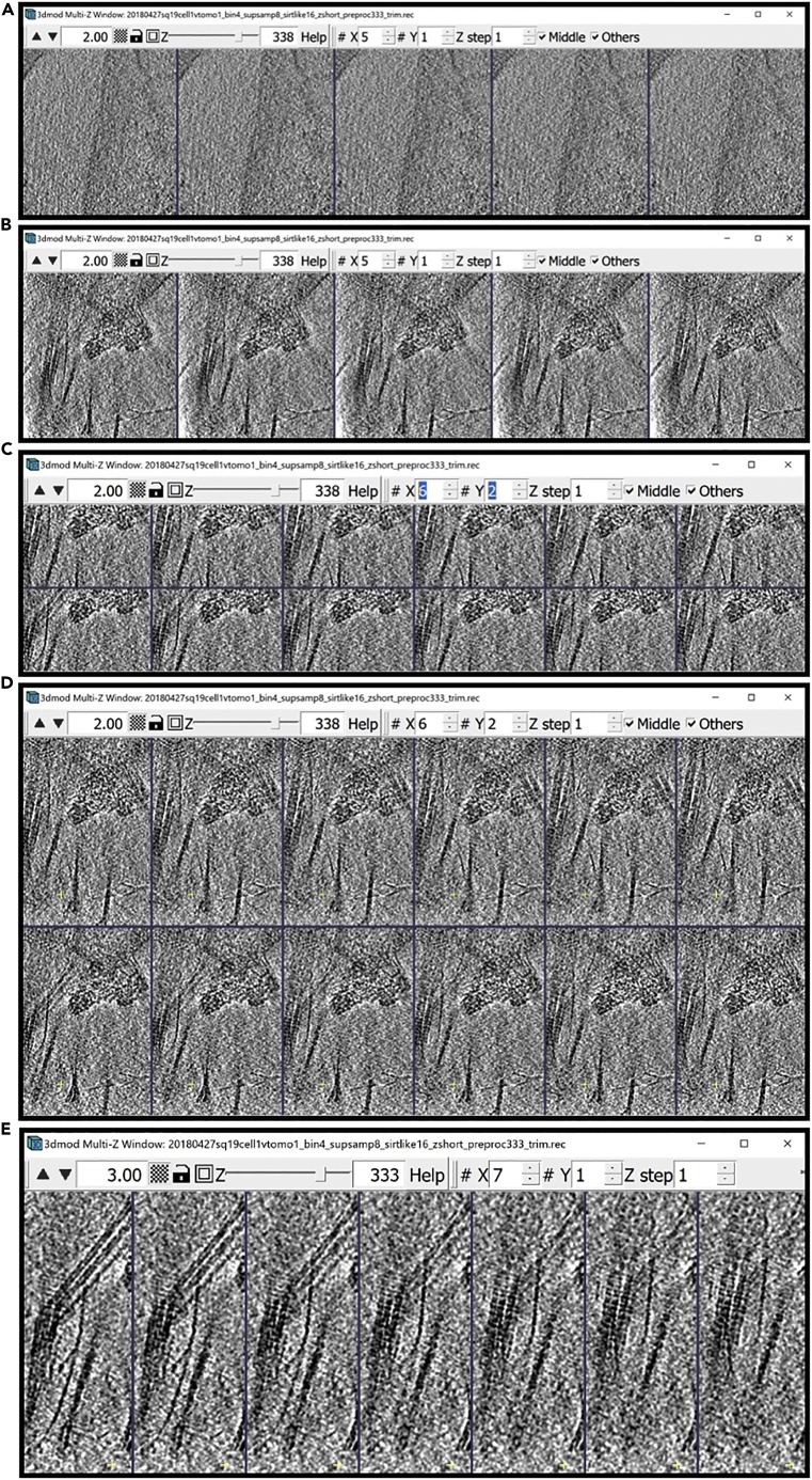
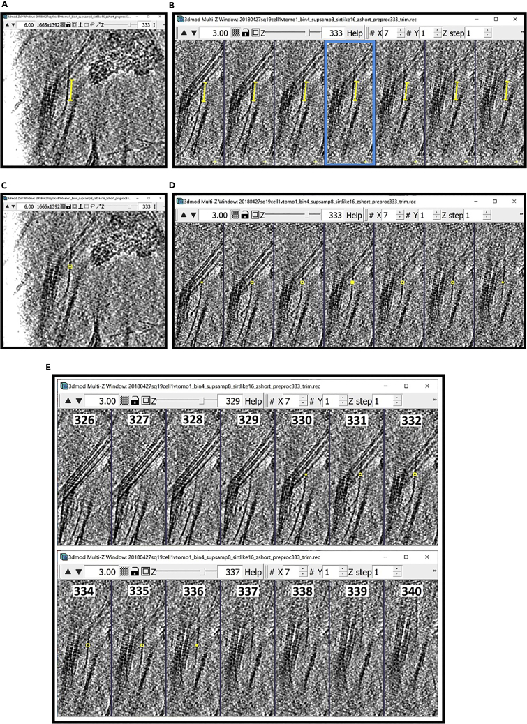
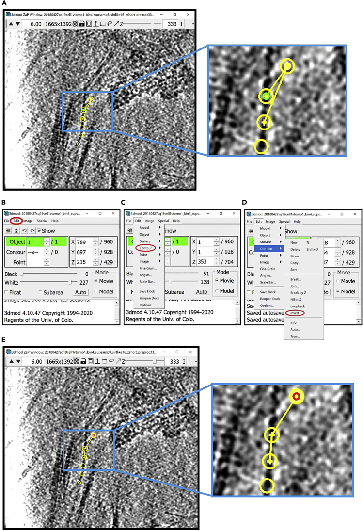
Note: While discussing filtration of tomograms is also out of the scope of this protocol, it is typically easier to perform annotations on appropriately filtered data. Given the wide range of data types this protocol may be applicable to (from soft X-ray tomography to scanning and transmission electron microscopy datasets, either at room or cryogenic temperatures), there is no one-size fits all recommendation we can provide. Here, the datasets we exemplify the protocol with from Dudek et al. (2021) had been subjected to low pass, high pass, and thresholding filters in EMAN2 (Tang et al., 2007) to further denoise the tomograms after binning and facilitate annotation. IMOD should allow for comparable functionality through its mtffilter algorithm and other scripts, documented on the man pages and the User’s Guide (see key resources table). There are more complex regularization (Maiorca et al., 2014) (Gontard, 2015), artifact removal (Fernandez et al., 2016), and denoising techniques also available such as linear diffusion, non-linear diffusion, and bilateral filters, among others (Maiorca and Rosenthal, 2018), some of which may even be applied directly to the tilt series before tomographic reconstruction (Maiorca et al., 2012). Optimal filtration will depend on the nature of each dataset and filtering requirements might be particularly different if working with negative-stain or phase plate data (Malac et al., 2021).
Open IMOD windows
Timing: 5 min
This section provides guidance to open IMOD and the necessary IMOD windows.
-
5.
After the tomogram is binned and filtered, you can open the tomogram from the terminal using the following command to inspect whether the contrast is optimal (make sure to replace file_name.mrc with the file name of the tomogram you want to annotate features in):
>3dmod file_name.mrc
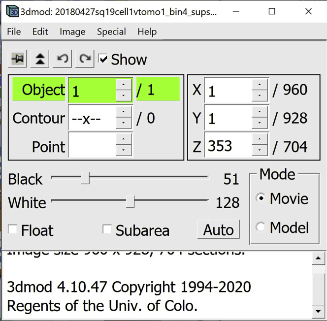
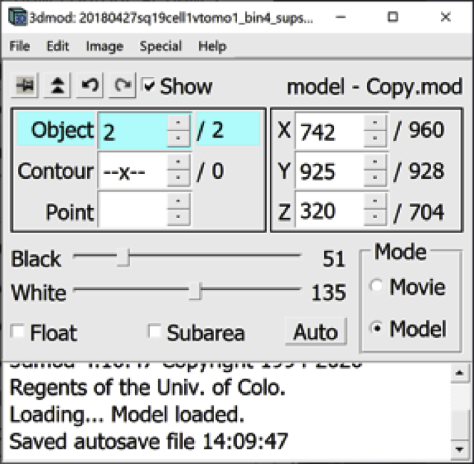
Two windows appear on the screen: the main 3dmod control panel, which we will hereafter call 3dmod Information Window, or simply “Information Window”.
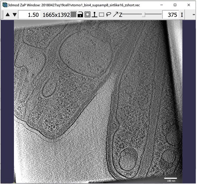
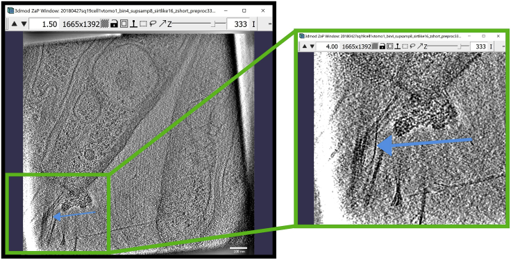
and the 3dmod “Zoom and Pan” (ZaP) Window that displays tomogram slices (Figure 1).
Note:Figure 1 contains a scale bar (100 nm) to give an idea of the physical size of the features shown. In the tens of dozens of images below, some may contain scale bars as a reminder of scale, but others may be missing them in the interest of minimizing clutter in the figures. Ultimately, the scale of a feature does not impact its annotation; thus, in the context of this Protocol, scale bars are largely irrelevant. A pixel is annotated in the same exact way whether it represents a physical size of 1 nm or 10 nm or 100 nm.
-
6.
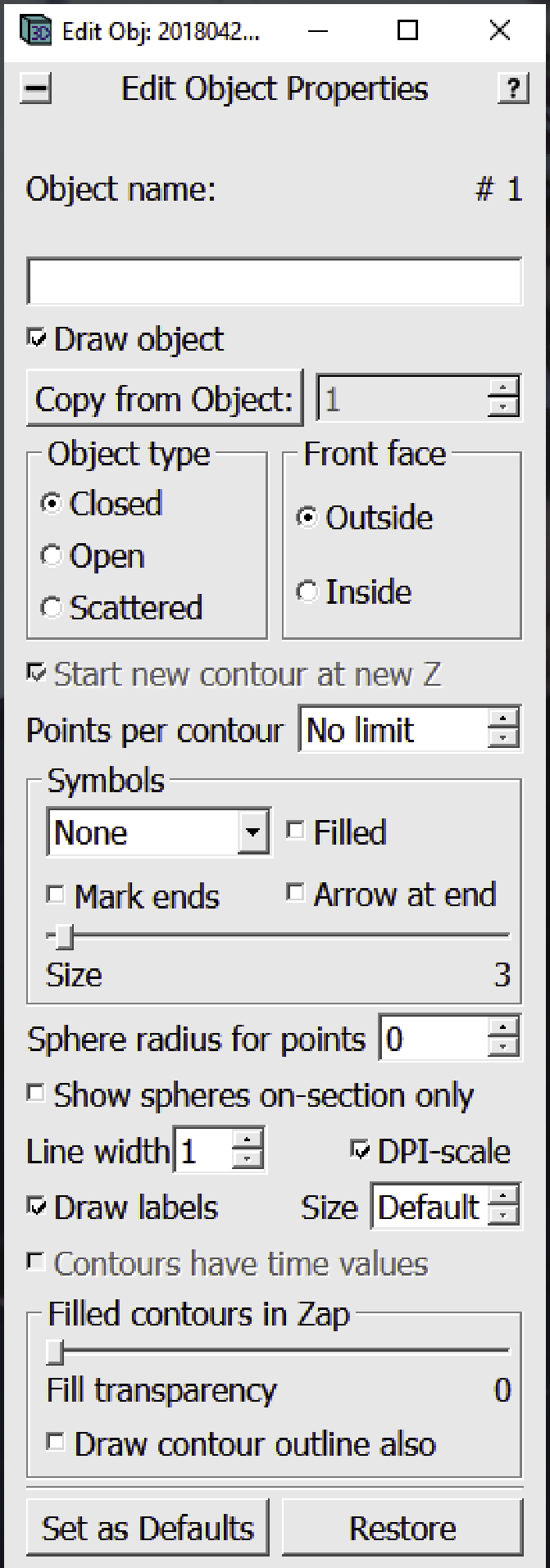
For annotation, we will need several other windows open. First, open the Edit Object Window. In the Information Window, find the menu at the top of the window and click on “Edit”. In the drop-down menu, hover your mouse over “Object” and click on “Type”.
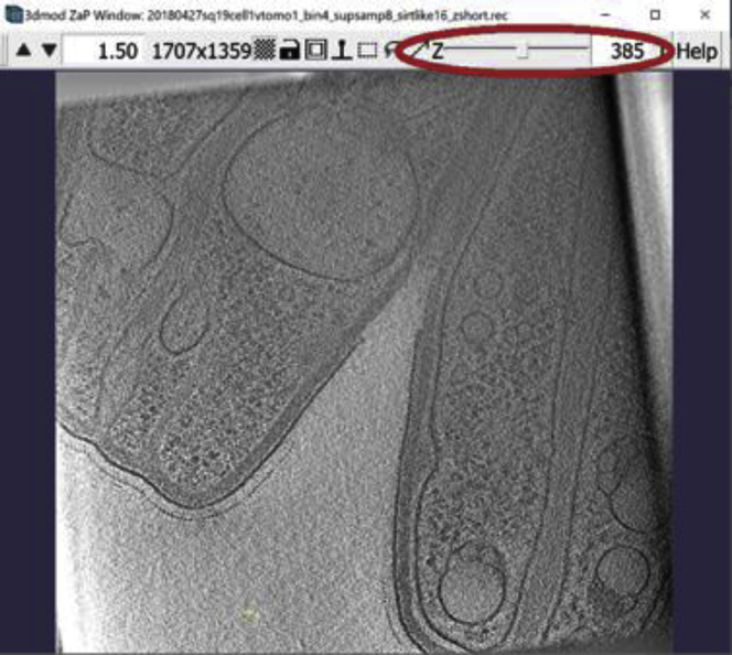
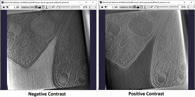
Figure 1.
3dmod ZaP window
The 3dmod Zap window displays a slice (∼1.5 nm thick) through a representative cryo-ET tomogram of a rectangular cell-like unit that appears to be “dividing”, showing multiple complex layers at the cell’s edge (this specimen is more fully documented in Dudek et al., 2021).
The Edit Object Window will appear on the screen.
-
7.
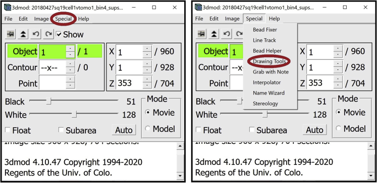
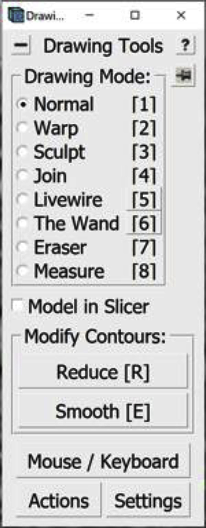
Open the Drawing Tools Window. In the Information Window, find the menu at the top of the window and click on Special. In the drop-down menu, click on Drawing Tools.
The Drawing Tools Window will appear on the screen.
-
8.
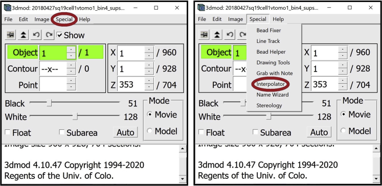
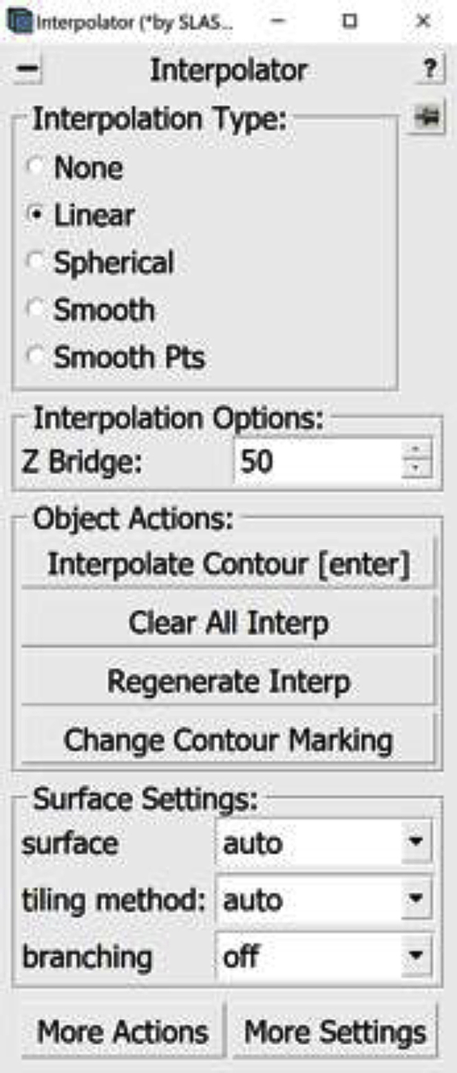
Open the Interpolator Window. In the Information Window, find the menu at the top of the window and click on Special. In the drop-down menu, click on “Interpolator.” In general, as in the panels below, parts of windows encircled with a red oval highlight the locations of options to select/click/modify.
The Interpolator Window will appear on the screen.
-
9.
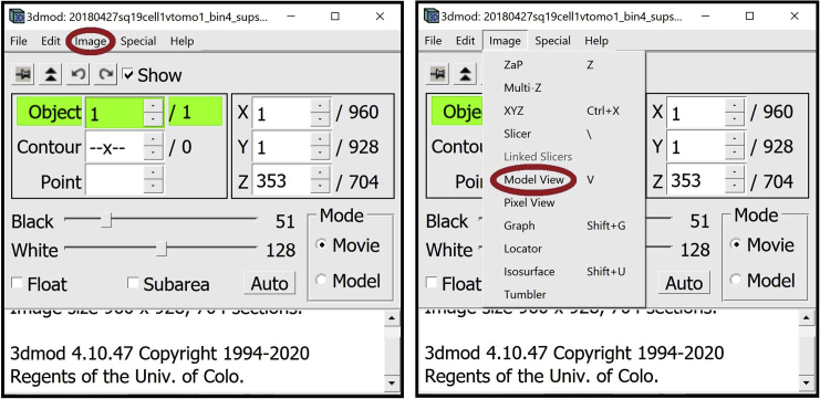
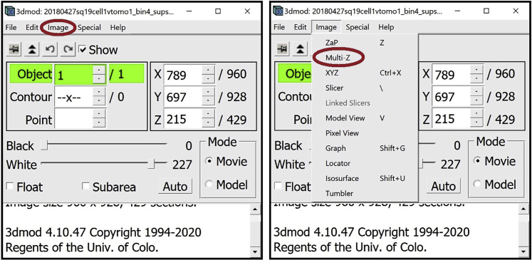
Open the Model View Window. In the Information Window, find the menu at the top of the window and click on Image. In the drop-down menu, click on “Model View.” Alternatively, you can open the window by pressing V key on your keyboard.
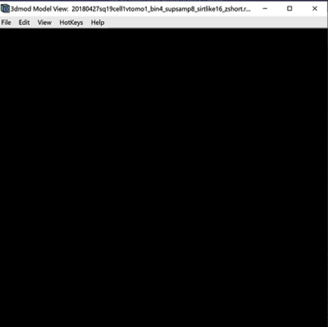
The Model View Window will appear on the screen (initially just showing an empty, black display as shown below since no tomogram has been loaded yet in this example).
-
10.
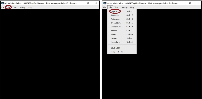
Open the Model View Object Editing Window. In the Model View Window, find the menu at the top of the window and click on “Edit.” In the drop-down menu, select “Objects…”. Alternatively, you can open this window using the Shift + O command.
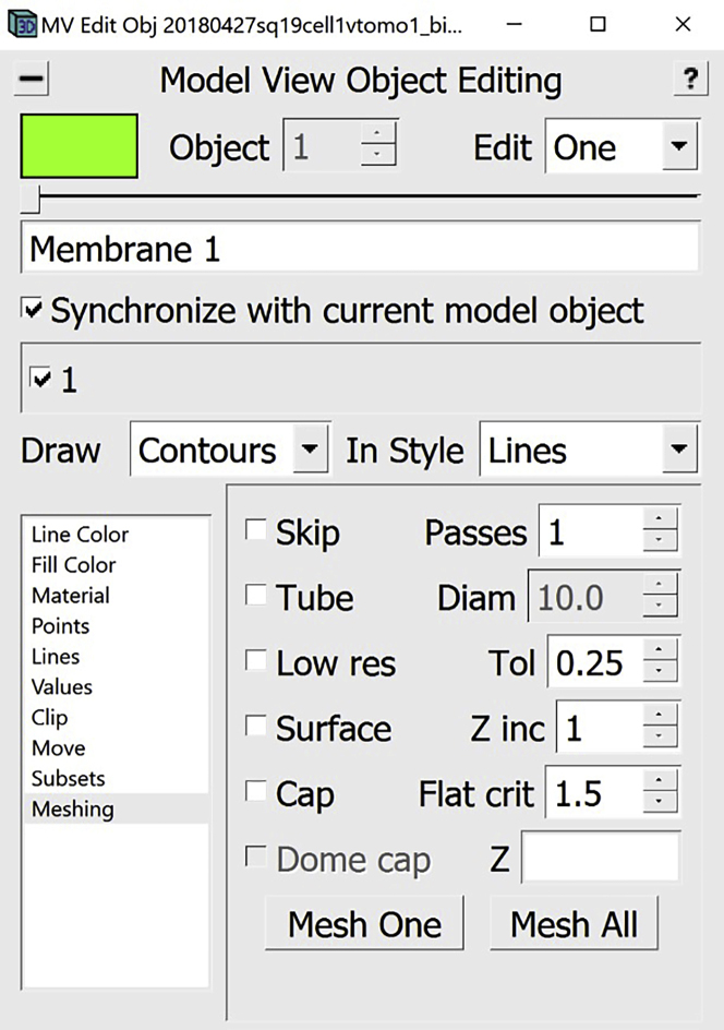
The Model View Object Editing Window will appear on the screen.
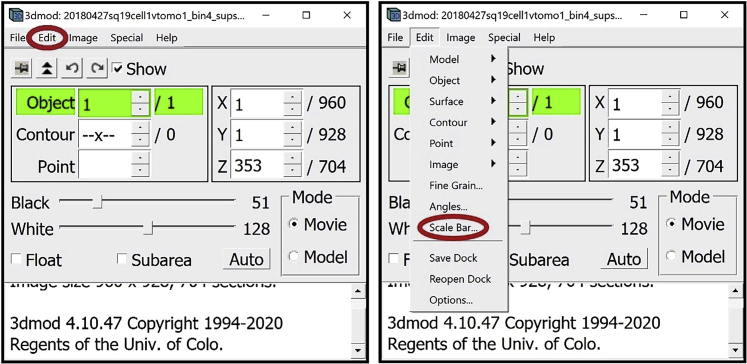
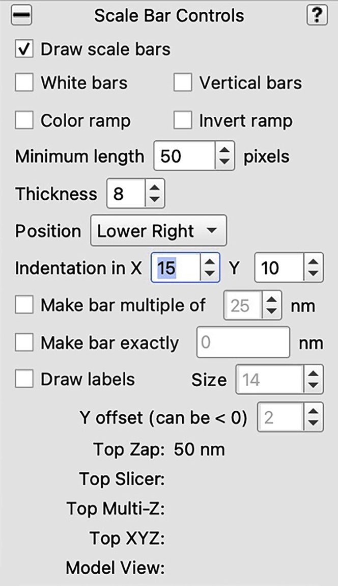
Optional: If you want to display a scale bar, in the Information Window, find the menu at the top of the window and click “Edit.” In the drop-down menu, select “Scale Bar…”.
The Scale Bar Window will appear on the screen.
Key resources table
| REAGENT or RESOURCE | SOURCE | IDENTIFIER |
|---|---|---|
| Deposited data | ||
| Tomogram in EMDB | Scientific study: Dudek et al. (2021), https://www.biorxiv.org/content/10.1101/2021.10.23.465578v1 | EMDB: 25419, https://www.emdataresource.org/ |
| Software and algorithms | ||
| Operating System – Linux/MacOS/Windows | This paper: Windows 10 | N/A |
| IMOD version 4.10.47 | Online | https://bio3d.colorado.edu/imod/ |
| IMOD User’s Guide | Online | https://bio3d.colorado.edu/imod/doc/guide.html |
| RAM memory – enough to open tomogram | This paper: 4 GB | N/A |
| Other | ||
| Mouse hardware | Any mouse with 3-button functionality | N/A |
| CPU – Any modern CPU | This paper: 2.4 GHz 8-Core Intel Core i9 | N/A |
Step-by-step method details
Below, we provide step-by-step instructions to manually annotate three different types of features: 1) membrane-like structures, 2) vesicle-like structures (globular-looking structure), and 3) tubular structures.
Annotating membrane-like structures
This method is for annotating and segmenting membrane-like structures. These may include but are not limited to long and relatively thin surfaces or layers, such as inner and outer bacterial membranes, peptidoglycan layers, s-layers, lipid vesicles, nuclear envelope, mitochondrial outer membrane and folded inner membrane forming cristae, etc. In this example, the annotation will delineate the inner membrane only. As the same procedure can be used for annotating the outer and inner membranes and other layers of a cell, for each annotation, you would choose one instance of a membrane at a time that you can trace through the slices of the tomogram. If there is a double membrane, do each membrane separately: first, the outer membrane, then the inner membrane, or vice versa. In this protocol, each instance of a membrane-like structure that we will annotate will be called an “Object”, and you can see the number of the Object you are working on in the Information Window.
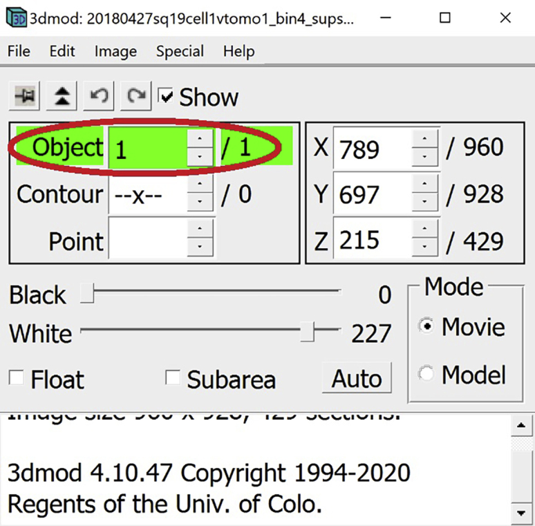
Setting up IMOD windows
Timing: 2 min
This section will guide the User to properly set up all the IMOD windows that will be used during annotation.
-
1.
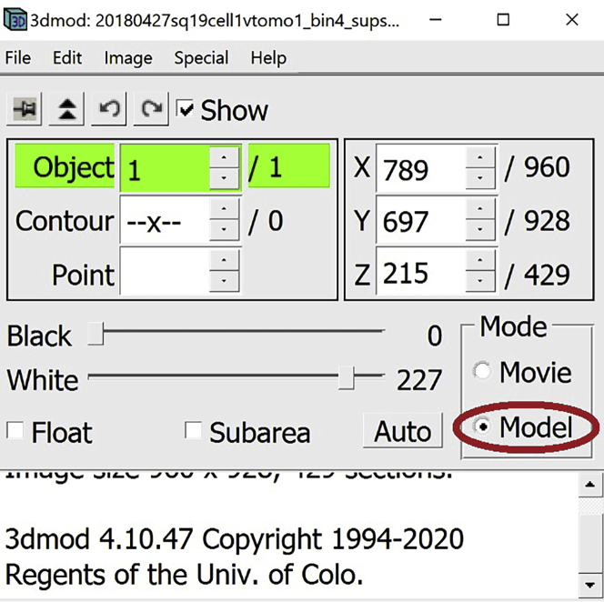
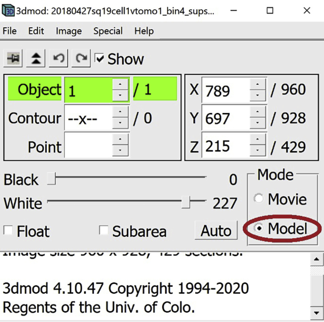
In the Information Window, select Model.
-
2.
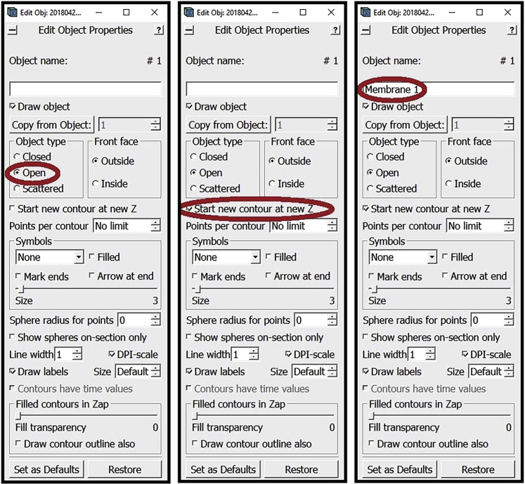
Go to the Z-slice where you want to start annotating the membrane (while you can start from the highest or lowest Z-slice where the membrane is visible, we recommend starting approximately in the middle where features tend to be the most clear, but it doesn’t really matter as this should not impact the end results). In the Edit Object Window choose as Object Type Open. In the Edit Object Window check the box next to Start new contour at new Z. Also in the Edit Object Window, choose a name for the Object and write it in the area under Object name (e.g., “Membrane 1”, you can choose any distinct name you want for each separate Object).
Manual annotation
Timing: < 30 min
This section will cover annotation of the chosen feature at different Z-slices in the tomogram.
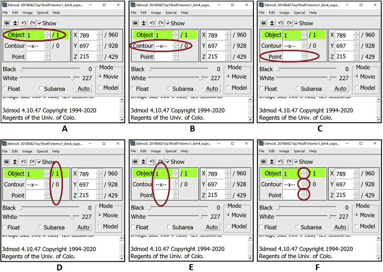
Note: Each instance of a continuous membrane-like feature will be an Object (panel A below). Each Object will be made of multiple Contours (panel B below), where each individual Contour will be composed of multiple Points (panel C below). The number of total Objects, Contours and Points appears in the column on the right (panel D below), and the number of the currently selected Object, Contour and Point appears in the column in the middle (panel E below). To change the selected Object, Contour or Point, you can use the arrows to the right of the middle column (panel F below).
-
3.Before we start making Points, Contours and Objects for our actual target annotations, we need to know how to create, access, change, and delete Points. Below, we will exemplify these operations on a largely “empty” area of a cryo-ET tomogram where the features correspond mostly to background noise.
-
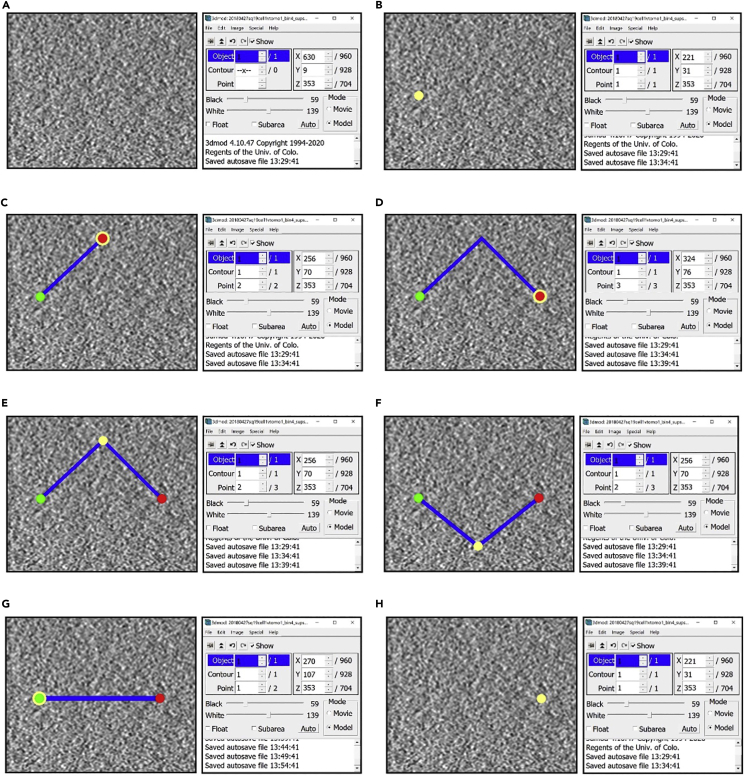
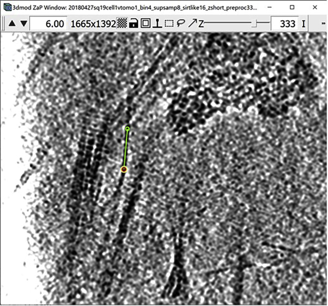
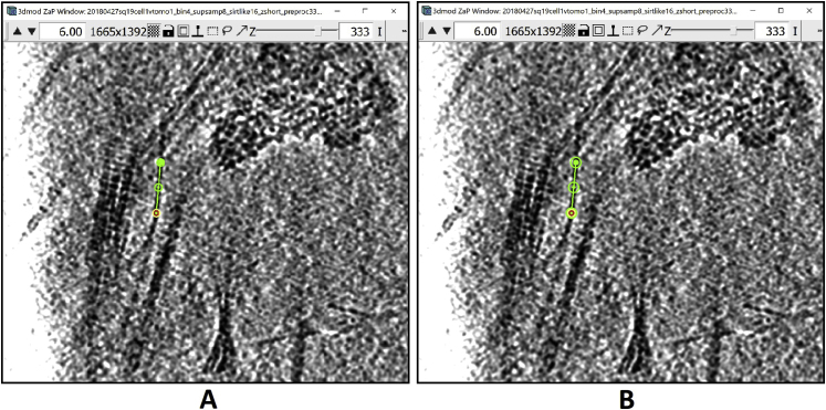
a.At the outset, there is one empty Object already by default with no Contours and no Points (Figure 2A).
-
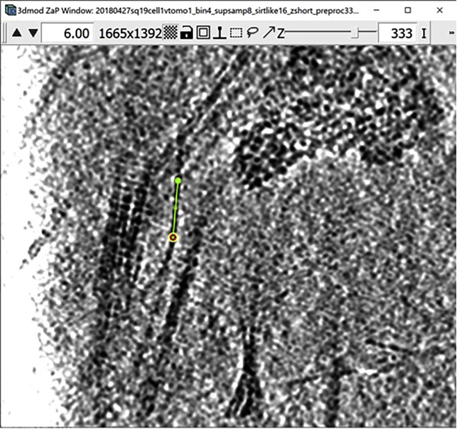
b.Middle clickto create your first Point. When working with an Object that has no Contours, creating a Point will automatically create the first Contour as well. Notice that the numbers in the Information Window below have changed to indicate that there is now one Contour with one Point as part of Object 1. The newly created Point always becomes the currently selected Point, which is why in the middle column we have 1 for the currently selected Object, Contour and Point. The Point created is yellow. The yellow color of a Point in a Contour highlights it as the currently selected Point (Figure 2B).
-
c.Middle click again to create a second Point in the first Contour of the first Object. The number of this newly created Point is 2. Notice that the Points of a Contour are sequentially joined by a line; the line of the Contour connects Point 1 to Point 2, then Point 2 to Point 3, and so on and so forth. The Point created is red and the previous point becomes green. The green color of a Point in a Contour indicates that it is the first Point of the Contour. The red color of a Point in a Contour indicates that it is the last Point of the Contour. Since Point 2 is both the currently selected Point and the last Point of the Contour, it is red with a yellow outline (Figure 2C).
-
d.Middle click again to create a third Point in the first Contour of the first Object. The number assigned to the new Point in the Information Window is (predictably) 3. As before, the newly created Point is red with a yellow circle surrounding it because it is the currently selected Point as well as the last Point in the Contour. The first Point of the Contour remains green. Notice that Point 2 is not marked. Any Points in the Contour that are not currently selected and are not the first or last Points of the Contour are not marked under the default settings of IMOD (Figure 2D).
-
e.Hover the mouse above the position of Point 2 and left click to select the Point. This action changes the currently selected Point. Another way to select a different Point is to use the arrows to the right of the middle column in the Information Window (Figure 9F above) to change the number of the selected Point. The yellow Point is now Point 2, because it is selected. Point 3 remains, red as it is the last Point of the contour, and the first Point of the contour, Point 1, remains green (Figure 2E).
-
f.Move the mouse somewhere below the second Point, then right click to move the currently selected Point. This action changes the position of the currently selected Point to the location pointed to by the mouse. This action does not change the numbers assigned to the Points in the Contour, and it does not change the location of any of the other Points. As before, Point 1, the first Point in the Contour, is green, and Point 3 is red, being the last Point of the Contour. Point 2 remains yellow since it is still the currently selected Point; however, its location changed. Note that you can see the three-dimensional (3D) X, Y, Z coordinates of any given Point in the right column of the Information Window (Figure 2F).
-
g.Press Backspace to delete the currently selected Point. You can use this to eliminate misplaced Points. This action deletes the second Point; it also updates the numbers assigned to the Points following Point 2 to indicate the new order of the Points. Hence, Point 3 now becomes Point 2. If there were more points following Point 2, the numbers of all of the Points would go down by one after Point 2 is deleted. Since Point 3 (the former last Point of the Contour) is now Point 2, Point 2 is now highlighted in red. Point 1 remains green since it is still the first Point in the Contour. Notice that deleting the former Point 2 changed the currently selected Point to the Point preceding it, Point 1. Therefore, Point 1 is now the first Point in the Contour as well as the currently selected Point, so it is green with a yellow circle surrounding it (Figure 2G).
-
h.Press Backspace again to delete the currently selected Point. This action deletes Point 1. Now the first Contour of the first Object has only one Point, which is the currently selected Point (colored yellow, as expected) as well as the first and the last Point of the Contour (Figure 2H).
-
a.
Figure 2.
Manipulating points
(A) Empty Object.
(B) Object after creating one Point.
(C) Object after creating a second Point.
(D) Object after creating a third Point.
(E) Object after selecting the second Point.
(F) Object after moving the second Point.
(G) Object after deleting the second Point.
(H) Object after deleting the first Point (Figures come in pairs, with the figure on the left showing a section of a slice of a cryo-ET tomogram mostly devoid of features (i.e., showing background noise) displayed in the ZaP Window with the points added, and the figure on the right showing the corresponding Information Window with Object, Contour and Point information).
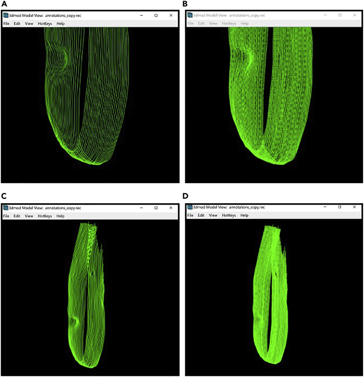
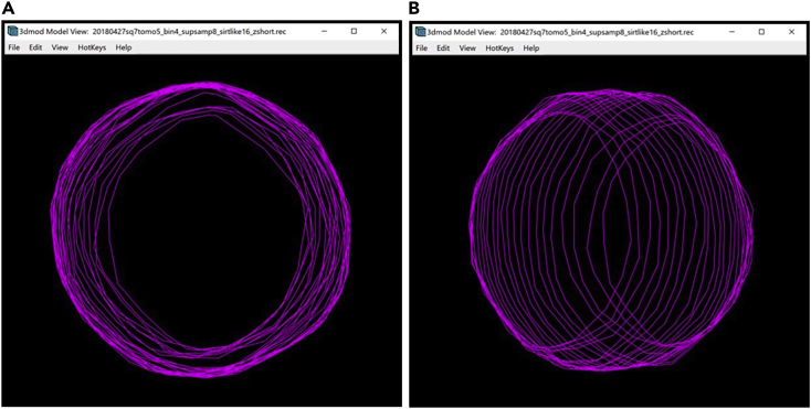
Figure 9.
Model of the target membrane displayed in the Model View Window
(A) Bottom section of the membrane without interpolated Contours.
(B) Bottom section of the membrane with interpolated Contours.
(C) The entire target membrane without interpolated Contours.
(D) The entire target membrane with interpolated Contours.
Tip: You can delete misplaced Points with Backspace as specified above, or you can delete an entire Contour by selecting it in the Information Window and pressing Backspace.
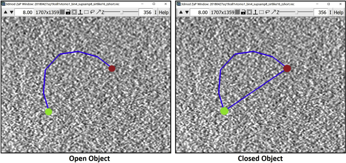
Note: As established above, a Contour is a line sequentially connecting multiple Points; i.e., a line that connects Point 1 to Point 2, Point 2 to Point 3, Point 3 to Point 4, and so on and so forth. Open and closed Objects both contain this line, with the only difference between them being that in closed Objects the last Point also connects to the first Point, thus creating a loop, while in the open Objects the line remains disconnected at the ends. For the annotation of membrane-like structures, we will be working with open Objects.
-
4.
Now that we know how to manipulate Points, we can create the first Contour. In the ZaP Window, slide the Z-slice slider and find a slice close to the middle of the tomogram where the feature of interest is clearly visible (i.e., pick the slice closest to “the middle” of the feature’s span in Z where you can see the feature most easily; note that accurate manual annotation is heavily dependent on being able to distinguish the feature of interest; if you have a hard time distinguishing the feature of interest, it may not be annotatable); we will annotate both the lower and the higher Z-slices later. The goal is to add Points along the membrane shown in Figure 3 below to create a Contour that approximates the membrane’s shape (that is, a Contour that overlaps as best as possible with the membrane, which corresponds to the dark, linear, sometimes curved pixel values in Figure 3; this will become ore clear as the annotation progresses). Since the line between two points is always straight, you need to choose the distance between two annotation Points so that it approximates the membrane’s curvature; therefore, if a membrane region is smooth and relatively straight, the distance between the Points can be bigger than if the membrane has creases, invaginations, bulges, or folds in general. This is a qualitative decision made for each instance that is to be annotated and is left at the discretion of the annotator depending on the desired precision.
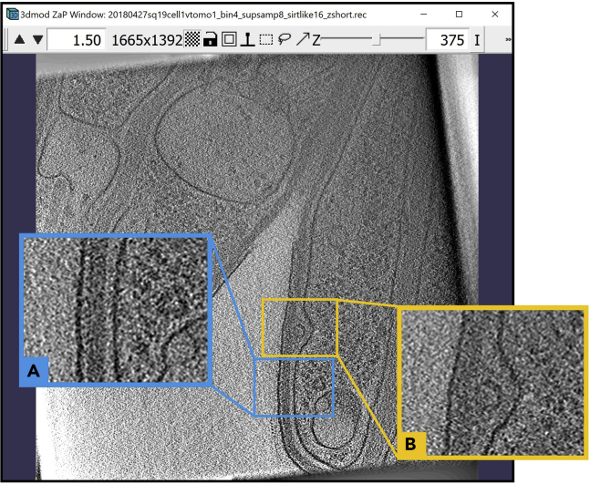
Note: Below are two portions of a cellular cryo-ET tomogram z-slice (Figure 3) with several membranous structures/layers separating the extracellular space from the cytoplasm The first example (Figure 3A) shows relatively straight and parallel layers while the second one (Figure 3B) shows the innermost layer curving inwards.
Figure 3.
Cryo-ET tomogram z-slice displayed in the ZaP Window
(A) Largely straight membrane section.
(B) Curved membrane section.
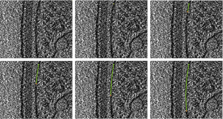
The panels below show how to create the Contour of the first membrane, showing what the Contour looks like after adding a few Points sequentially. The Points are added at an interval that can approximate the membrane’s shape. Since the membrane is relatively straight, we can create a Contour with only 5 Points.
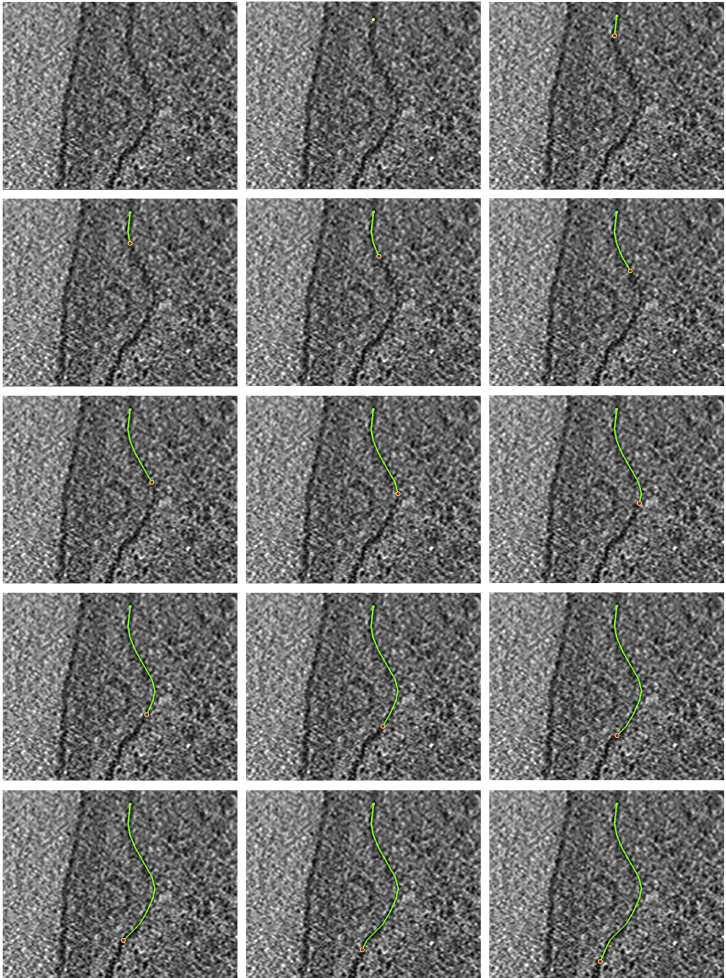
The second example contains a highly curved region in the “inner membrane”; hence, we will need more Points to approximate it. The panels below show how we can create a Contour with 14 Points.
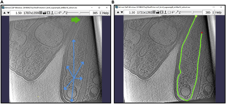
Now, we will annotate the inner membrane pointed to by the multiple blue arrows below, starting at the wide green arrow in the top part of the first image below (Figure 4A). On the right (Figure 4B), we show the same Z-slice after completing the annotation.
-
5.
For a more accurate annotation, we will zoom in to the portion of the membrane that we are annotating using the arrows at the top of the ZaP Window.
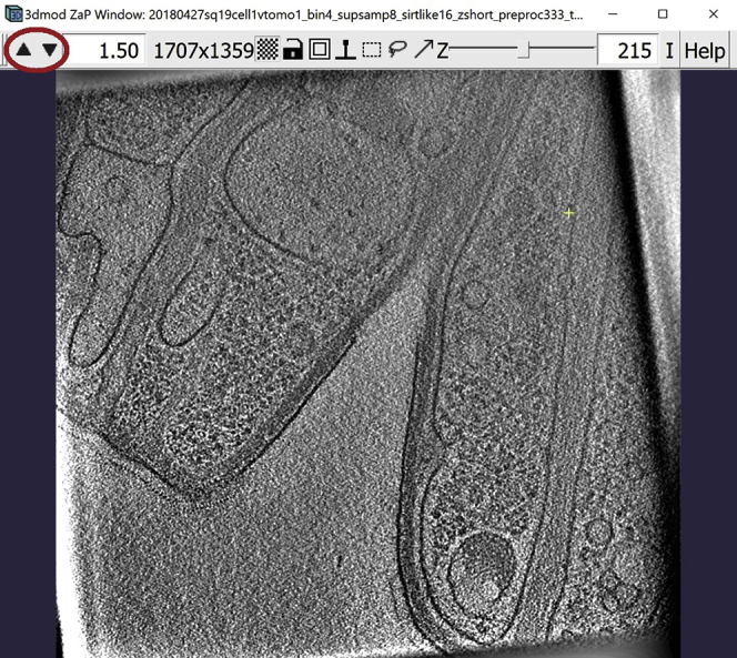
Figure 4.
ZaP Window displaying the slice 385 of a cellular cryo-ET tomogram
(A) The blue arrows indicate the target membrane and the green arrow indicate the starting point of the annotation.
(B) The finished Contour of the target membrane.
Zoom in to 4.0×. To move to a different X,Y location on the same Z-plane, Left Click and hold, dragging the mouse to navigate to the desired region.
-
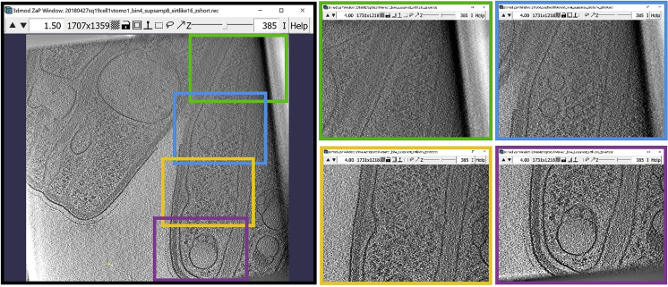
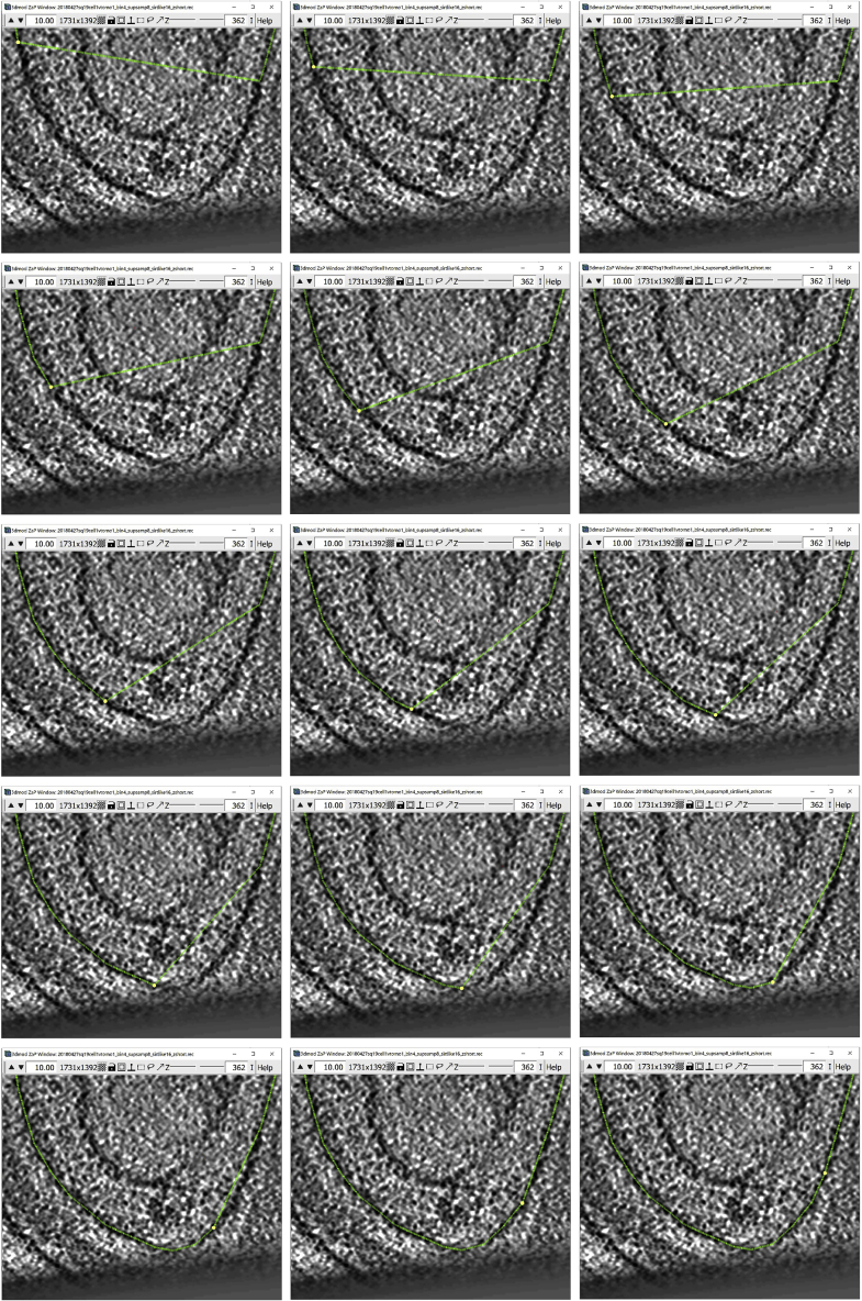
6.We will next work on the four regions depicted below (Figure 5). Since we will start from the top of the slice and work our way down, we will first zoom into the region highlighted with a green square outline, and then move to the blue, orange, and purple regions, annotating along the way. When we reach the bottom-most point, we will continue the same process on the other half of the membrane, navigating to the same regions in a reverse order. This process is explained in more detail below.
-
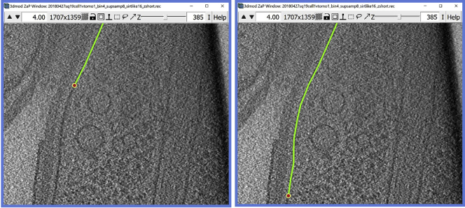
a.We will first zoom in to the green region and start by adding the first Point at the location indicated by the green arrow. In your own dataset, you can start at a point where the chosen membrane-like structure becomes visible on the Z-slice, either at the boundary of the tomogram (as below) or at an “edge” of the structure. We then add more Points along the membrane until we reach the bottom boundary of the zoomed-in region, as shown in the panels below starting at the green arrow (the panels progress from left to right).
-
b.When we reach the bottom of the zoomed in region, we move to the next region by holding Left Click. In our example, we will transition from the green region to the blue region; however, when working on your own dataset, simply move to a new region along the chosen membrane-like structure to continue annotating it. Below, we continue annotating the membrane until we have reached the bottom of the blue region.
-
c.Transition to the orange region and continue.
-
d.Transition to the purple region and continue annotating the membrane. In this region, the membrane curves back up. Continue annotating until you reach the top of the purple region again.
-
e.Return to the orange region, and continue annotating the membrane, now moving upwards. Continue annotating the membrane in the orange, blue and green regions, as shown in the panels below.

-
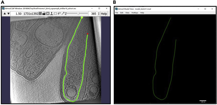
f.When the Contour has reached a Point where the membrane ends or cannot be seen on the slice anymore, the Contour is finished. Zoom out with the arrows on the top corner of the window (the ones you used to zoom in) and view your result (Figure 6A).
-
g.Navigate to the Model View Window to see the contour in 3D (Figure 6B).
-
a.
-
7.Now that we know how to create a Contour, we can continue adding other Contours at different Z-slices.Note: To navigate through the Z-slices, use the slider at the top of the ZaP Window. The number to the right of the slider indicates the number of the Z-slice that you are currently viewing, as shown in the image below.
-
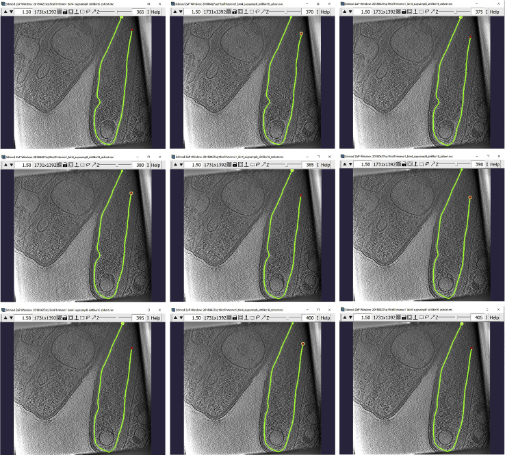
a.In this method, we do not have to annotate each slice. We will be skipping several slices that will later be filled in during step 2 using interpolation. For most features, you can typically skip between 4 and 10 slices. This number is chosen on a case-by-case basis: the less the membrane changes from slice to slice, the more slices we can skip. For other specimens or other data collection settings (e.g., higher or lower magnification, or a different amount of binning), the features may vary more rapidly or more slowly, such that fewer (a larger number of) or more (a bigger number of) slices can be skipped in between annotated slices.
 CRITICAL: The choice of the step size is very important. Be cautious not to choose a step size that is too big because it would result in more incorrectly interpolated Contours that will later have to be fixed. As a rule of thumb, it is always best to choose a smaller step size when not sure; however, a bigger step size chosen in appropriate situations will decrease the amount of work and time needed for the current step.
 -
b.In our example, we can skip 5 slices. So, if we start at 385 an create the first Contour there, we then navigate to the Z-slice 390 and create a new Contour for the same membrane, and afterwards we navigate to 395 and add a new Contour there too. Repeat the process to cover the entire range of slices over which the membrane is visible and traceable. The repeat the same process starting at Z-slice 385, except now go down the Z-slices to 380, then to 375, and so on and so forth, adding a new Contour at each selected Z-slice. For example, the panels below show nine Contours: the Contour at Z-slice 385, then four above and another four below it, separated by intervals of five slices (notice the z-slice number in the upper right corner, next to the slider bar).
-
a.
-
8.
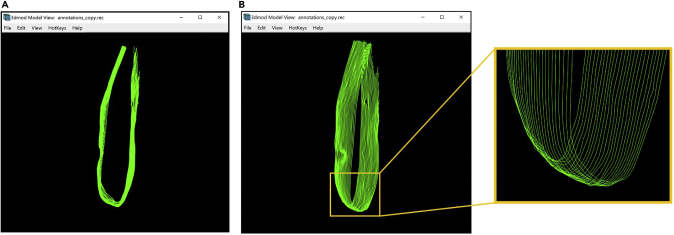
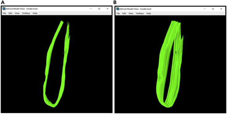
At this point you should have the Object named “Membrane 1” with several Contours that are equally spaced from each other. In this example, a total of 25 Contours were annotated for the inner membrane, covering from Z-slice 320 and going up to Z-slice 440. Navigate to the Model View Window and you can see in 3D the lines of the membrane that you traced, as shown in Figure 7A. An oblique and/or zoomed-in view as in Figure 7B more clearly shows the separation between individual contours.
Optional: Now that we have produced an initial model and have partially annotated the first feature of interest, pretend that you are done for the day, you want to wrap up, save the model and re-open it tomorrow.
Figure 5.
ZaP Window displaying a slice of a cellular cryo-ET tomogram with four regions of the target membrane boxed out in green, blue, orange, and purple
Figure 6.
The finished Contour of the target membrane
(A) ZaP Window view.
(B) Model View Window view.
Figure 7.
Model of the target membrane with manually drawn contours
(A) Top view of the model displayed in the Model View Window.
(B) Rotation around the y-axis of ∼40° with respect to the model in A, with a zoomed-in region highlighting the bottom of the annotation model.
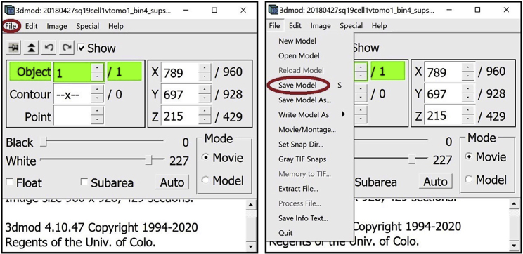
To save the current model, navigate to the menu at the top of the Information Window and click on File. In the drop-down menu select Save Model.
Alternatively, you can press the S key on the keyboard.
A window will appear where you can choose the destination and the name of the model to be saved. Preferably, the model should be saved as a .mod file.
To open a saved model, navigate to the menu at the top of the Information Window and click on File. In the drop-down menu select Open Model.
A window will appear where you can choose the file with your saved model.
Interpolation
Timing: < 1 h
For this step, we will be using IMOD’s Interpolator feature, which uses a built-in algorithm that when called on a Contour, compares the selected Contour either to the nearest Contours (in the first Z-slices upstream and/or downstream that have been annotated) or to all the Contours of the Object, and fills in Contours for the Z-slices where no manual Contours have been drawn. Thus, by using this function, we will interpolate between the Contours that we have completed manually already in order to fill out the Contours in the Z-slices that we skipped. This way, we can dramatically reduce the time needed for annotation by at least 5× for this example.
-
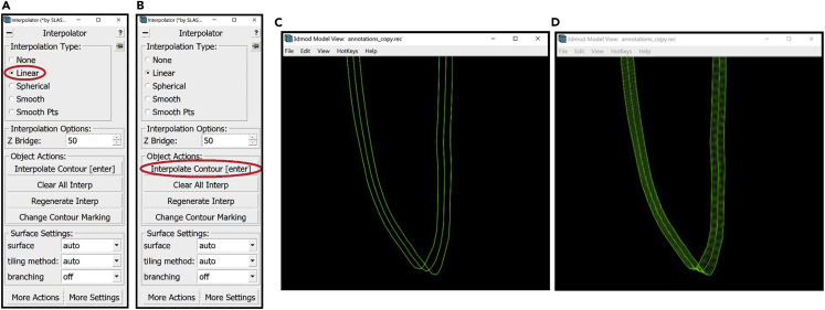
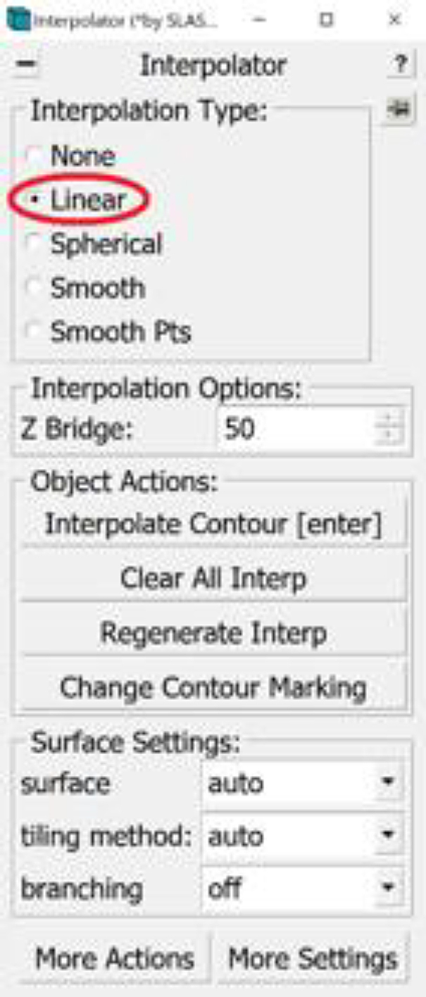
9.Select Linear under Interpolation Type in the Interpolator Window (Figure 8A).
-
10.
The linear interpolation only draws the Contours above and below the selected Contour, on Z-slices up to the next manual Contour at either end. For example, if we have manually drawn Contours at Z-slices 380, 385 and 390, and we interpolate on the Contour at 385, the algorithm will automatically “fill in” or trace similar Contours at the Z-slices 381–384 and 386–389. Therefore, to obtain a full, contnous annotation, we need to call the Interpolator on every other Contour that we have manually segmented. (There is a method to do Linear Interpolation synchronously on all the manually drawn Contours; this method is described later in this Protocol).
-
11.
In order to navigate between the Contours, you can either go through the Z-slices in the ZaP Window and left click on the Contour to select it, use the arrows next to the Contour number in the Information Window, or Right Click on the desired Contour in the Model View Window. Either way, the Contour number will indicate the selected Contour.
-
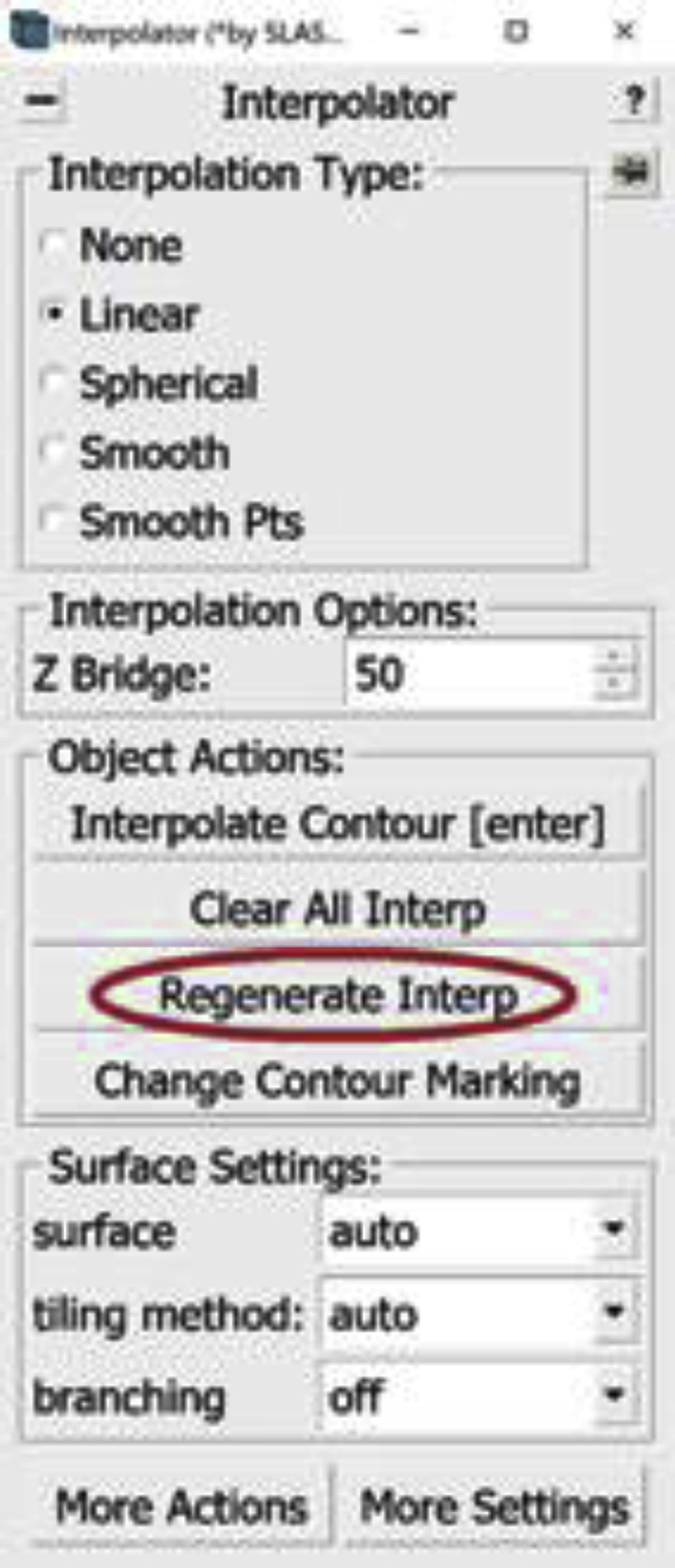
12.In order to interpolate at a selected Contour, press the Interpolate Contour button in the Interpolator Window (Figure 8B). Alternatively, you can just press the Enter button on your keyboard.
-
13.
The interpolated lines will appear in the ZaP Window at their respective Z-slices as well as in the Model View Window as a dashed line. For example, consider three Contours of the membrane we’re annotating: at Z-slices 380, 385 and 390. Select the contour at Z-slice 385 and press Enter. Figures 8C and 8D) shows the Model View Window zoomed-in to the bottom of the membrane before (Figure 8C) and after interpolation (Figure 8D).
-
14.
We can then interpolate the rest of the manually drawn Contours at every other level to complete all the missing Contours.
Optional: An alternative, faster way to use Linear Interpolation is to interpolate on all manually drawn Contours at the same time. To do that, we select a Contour of the Object of interest and press the Regenerate Interp button in the Interpolator Window (another window will pop up to confirm you want to regenerate all interpolations; press “yes”).
-
15.
Open the Model View Window to view the finished annotation of the target membrane (Figure 9).
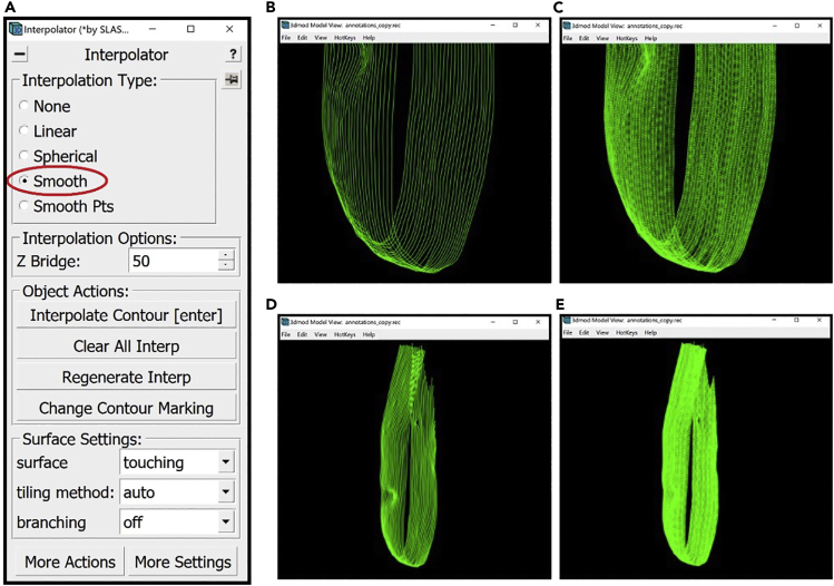
Optional: An alternative to Linear Interpolation is Smooth Interpolation. For this method, select Smooth under Interpolation Type in the Interpolator Window (Figure 10A).
Figure 8.
Linear interpolation
(A) The location of the “Linear” Interpolation Type in the Interpolator Window circled in red.
(B) The location of the “Interpolate Contour” button in the Interpolator Window circled in red.
(C) Model View Window displaying the bottom of the model before interpolating on the middle Contour containing three manually drawn Contours.
(D) Model View Window displaying the bottom of the model after interpolation containing three manually drawn Contours and interpolated intermediate Contours.
Figure 10.
Smooth interpolation
(A) The location of the “Smooth” Interpolation Type in the Interpolator Window circled in red.
(B) Bottom section of the membrane without interpolated Contours displayed in the Model View Window.
(C) Bottom section of the membrane with interpolated Contours displayed in the Model View Window.
(D) The entire target membrane without interpolated Contours displayed in the Model View Window.
(E) The entire target membrane with interpolated Contours displayed in the Model View Window.
The smooth interpolator draws all the missing Contours in between the existing Contours of the Object at once. Therefore, you can choose any manually drawn Contour, click on Interpolate Contour in the Interpolator Window, or Enter on the keyboard. You can then open the Model View Window to view the finished annotation of the target membrane (Figures 10B–10E).
The two methods yielded a very similar result, so it does not seem to matter which one we choose, except that smooth interpolation involves fewer clicks. Thus, for the membrane shown, we used smooth interpolation. We hypothesize that sometimes one interpolation method might yield a better result than the other in approximating the membrane; however, we have never noticed any relevant qualitative differences for the examples shown in this Protocol. You may want to try both and see which one is more suitable for your target features, in case there is a difference for your specimen.
-
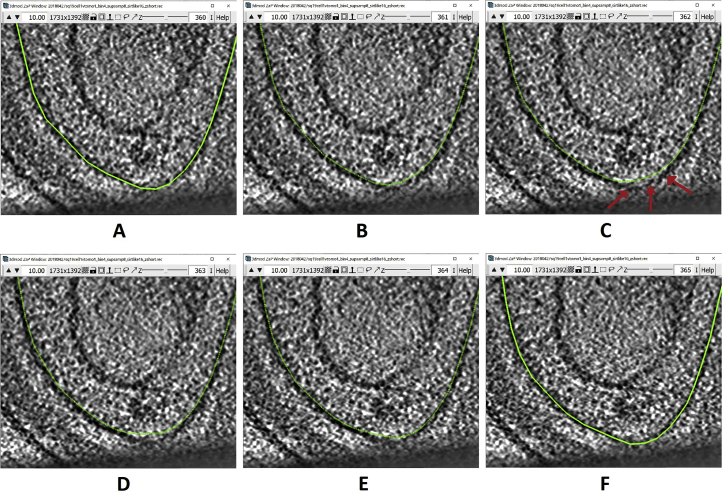
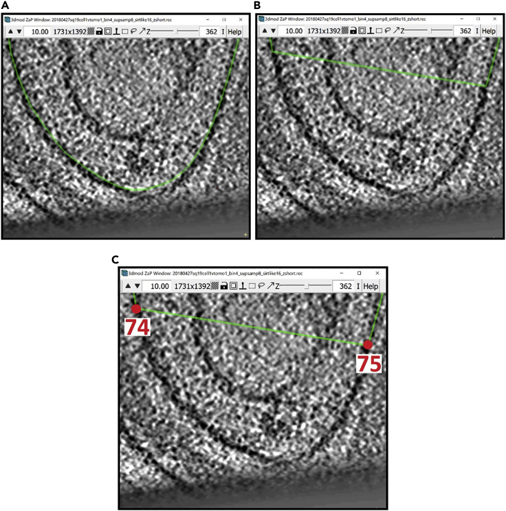
16.Some interpolated lines might not be very accurate irrespective of the interpolation method used. They could go beyond the membrane or be too short and not cover the entire membrane. The areas that tend to be most problematic are curved areas or areas at either tip of the Contours. The panels below show an example of this in a range of tomogram slices from z=360 (panel A) through z=365 (panel F), highlighting a particularly problematic area in the slice at z=362 (panel C), as indicated by the red arrows:The Contours at Z-slice 360 and 365 have been manually drawn, while the ones between them were interpolated. Notice how the interpolated Contours go a bit above the actual membrane on every interpolated slice (but not the manually drawn ones; i.e., A and F); on Z-slice 362 the problematic region is pointed to by three red arrows. You can edit these interpolated lines to correct problems within them using different tools from the Drawing Tools Window, as shown in the example below. Here I will mention the one that I found most useful and will show how to use it to correct the interpolated line at Z-slice 362. You can navigate between the Drawing Modes by selecting the mode in the Drawing Tools Window. Alternatively, you can press the corresponding key on the keyboard (1–8) to change between the Drawing Modes.
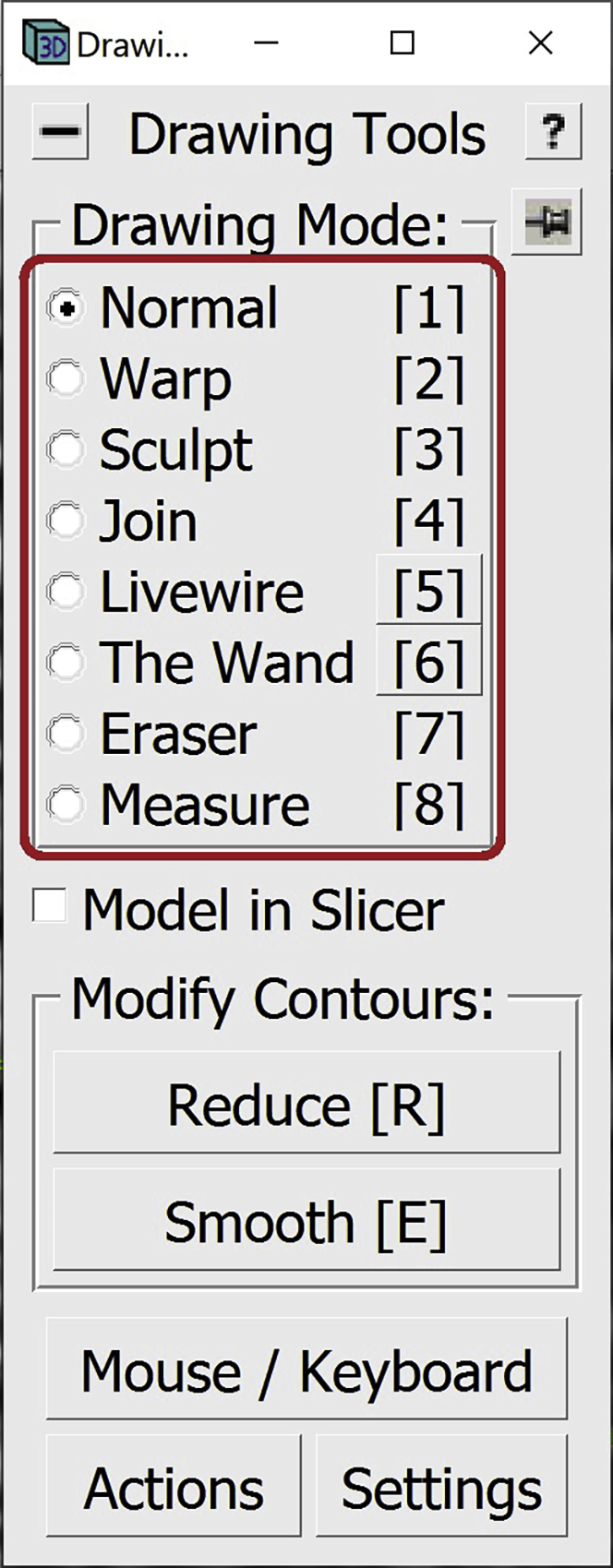
So far, we have been working in the Normal Drawing Mode. In this mode, you can edit Points as mentioned before; you can Middle Click to create new Points, Right Click to change the position of a Point, or press Backspace to delete a Point. When correcting a Contour, we can use all these tools to change the interpolated Contour.
The easiest method to use is to find the segment where the Contour is inaccurate, delete all the Points in that segment, and add new ones with Middle Click.
Let’s work on the Contour at slice 362 (Figure 11A).-
a.First, delete all the Points that are not following the membrane with the desired precision, which in this example will mainly be the Points where the membrane curves upwards (Figure 11B).
-
b.There is a Point at either end of the deleted segment. Find the Point that has a smaller number among those two by Left Clicking on them and checking the number of the Point that is displayed in the Information Window. In our example, the two Points are 74 and 75 (Figure 11C).
-
c.Select Point 74 and start adding Points with Middle Click just like before along the membrane, moving toward Point 75, as shown successively in the panels below (starting from the top left panel, going through left to right for each row, and top to bottom across rows, to end with the right bottom panel):
-
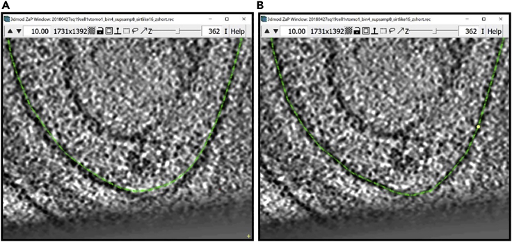
d.You can see the difference between the original interpolated Contour and the manually corrected in Figure 12.
-
e.Instead of correcting each interpolated Contour between the manually drawn Contours on the Z-slices 360 and 365 you can choose an interpolated Contour somewhere in the middle, correct it and then interpolate. This might automatically correct the other interpolated Contours between the slices 360 and 365, so as to prevent having to manually correct all four Contours. In the example above, after correcting the Contour on Z-slice 362, you can try pressing Enter on your keyboard, then check whether the newly interpolated Contours are accurate.Optional: There are other drawing modes that you can try using, such as Warp and Sculpt, as explained in a separate tutorial (Noske, 2011). Using Wrap and Sculpt modes typically yields Contours with a much larger number of Points than the method we present above, which will increase the file size of the model, and if working on a modest computer, this might introduce lag in the annotation process. However, with a powerful-enough computer, this should not be a problem, and you can use whichever mode you prefer.
-
f.After editing an interpolated dashed line, you might want to change it to a solid line, however this step is optional. To do that, select a Contour that has a dashed line. To change it to solid, you can press the Change Contour Marking button in the Interpolator Window.
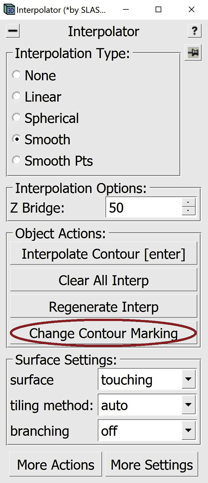 Alternatively, you can press Enter on your keyboard. This will change the marking of the line and will also re-interpolate on the selected Contour.
 CRITICAL: Correction of the interpolated Contours can be a critical step in the annotation of any structure, depending on the desired accuracy. Make sure to check all interpolated Contours to ensure that they follow the structure being annotated within your desired level of accuracy.
-
a.
Figure 11.
Bottom region of the membrane at z-slice 362 displayed in ZaP Window
(A) Interpolated Contour of the membrane.
(B) Interpolated Contour with deleted Points in the section that does not follow the target membrane.
(C) Interpolated Contour showing the numbers of the Points at either end of the deleted section.
Figure 12.
Bottom region of the target membrane showing the difference between the interpolated Contour before and after correction
(A) Bottom region of the interpolated Contour before correction.
(B) Bottom region of the interpolated Contour after correction.
Meshing and 3D visualization
Timing: <5 min/Object
In this step, we will be using the Model View Window as well as the Model View Object Editing Window. At this point, you should have the chosen membrane-like structure delineated in 3D in the Model View Window. Using the Model View Object Editing Window, we can now edit and manipulate the annotations to get a better visualization.
The first step is to mesh. Meshing will allow us to create 3D annotation objects that resemble the data more closely. For instance, the membrane is several pixels thick; however, in the Model View Window it appears as a thin line. To make the 3D membrane thick, we can mesh by creating a tube of the required thickness around each Contour. This will become clearer after the explanations below.
We start with the membrane (Figure 13).
-
17.Before we mesh, we need to find the thickness of the membrane.
-
a.To do that, navigate to the Edit Object Window. We will be working with the settings highlighted below.
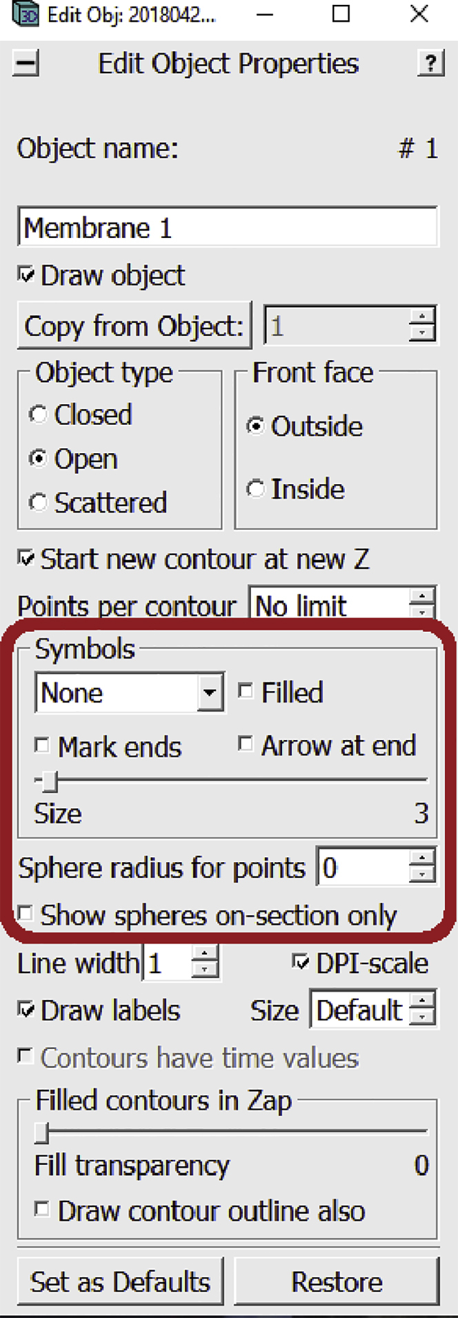
-
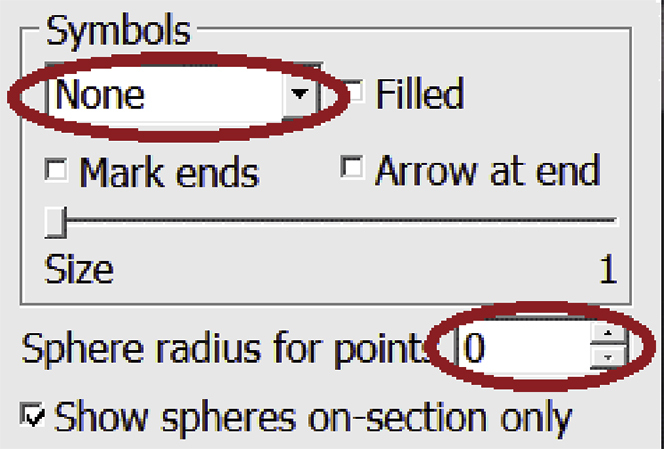
b.In the drop-down menu under “Symbols”, choose Circle. Check that the Size slider is adjusted to 1. Check the box next to Show spheres on-section only.
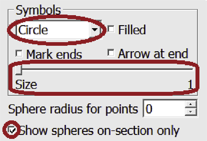
-
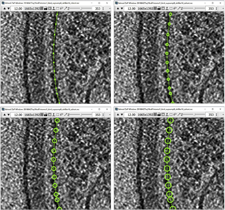
c.Next to Sphere radius for points increase the value to 1, then 2, then 3 and so on, using the up and down arrows to the right, as shown in the panels below.Do this until the diameter of the circles around the Points of the Contour look large enough (in the ZaP Window) to cover the entire thickness of the membrane, as shown in the panels below.
-
d.Find the radius of the sphere that is big enough to cover the thickness of the membrane. We can see above that a radius of 3 corresponds well with the actual thickness of the membrane; however, our Contours (and, in particular, the interpolated contours) might not always accurately line up with the midpoint of the membrane’s thickness along the entire membrane, so it might be best to use a radius of 4 if we want to cover the entire thickness.
 CRITICAL: Finding a suitable diameter for the membrane is an extremely important step. This will be important when you turn your annotation into a mask that you can use to produce a segmentation; that is, to extract the actual data densities of the annotated feature. Below, this will be done automatically with the IMOD program imodmop; however, the annotation model file can be manipulated as any other image (for example, to make the edges soft with a Gaussian expansion or a low-pass filter), and the masking operation may be carried out with other software.
 -
e.Note your chosen radius value (4 in this example); we will use it later. For now, change the settings back to how they were, with no circles drawn. Set the Sphere radius for points back to 0 and change the Symbol from the drop-down menu from Circle to None.
-
a.
-
18.We can now proceed to meshing.
-
a.Open the Model View Window and the Model View Object Editing Window.
-
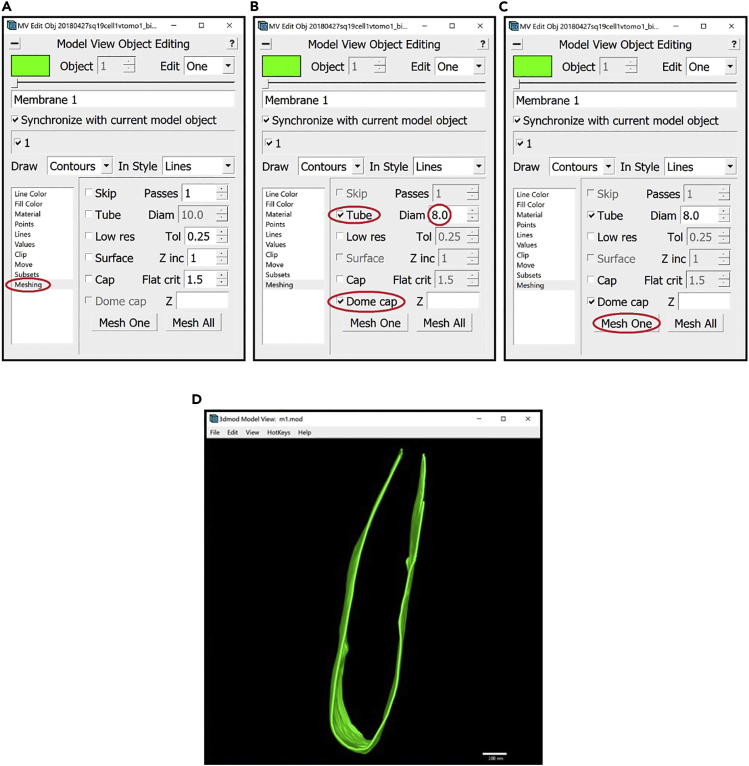
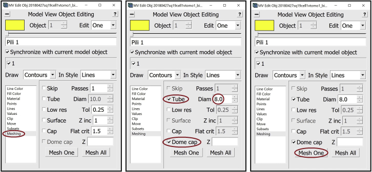
b.In the Model View Object Editing Window, in the menu on the left, select Meshing (Figure 14A). For membrane-like structures, we do meshing using the Tube option. In the Model View Object Editing Window, check the box next to Tube, then change the value after Diam to twice the “radius” that we found before, which in this case is 8 (since the radius was 4). Check the box next to Dome cap (Figure 14B). Now press the Mesh One button and see the results in the Model View Window (Figure 14C).
-
c.View the meshed membrane in the Model View Window (Figure 14D).
-
a.
-
19.Another useful feature of the Model View Object Editing Window is that it allows changing the colors of different Objects.
-
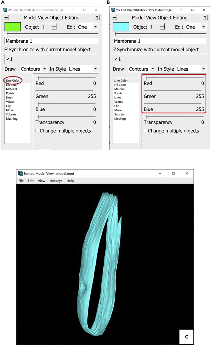
a.To do this, navigate to Line Color in the menu on the left of the menu (Figure 15A).
- b.
-
a.
-
20.At this point, we have completed the annotation of one of the inner membranes of this cellular sample. Now we will repeat the steps above to annotate all of the other inner membranes.
-
a.First, create a new Object. Each instance of inner membrane will be its own Object. Therefore, to annotate a new instance of inner membrane, we need to create a new Object for it. Open the Information Window. In the menu at the top of the window, press Edit. From the drop-down menu, select Object, then New.
-
b.Now there are two Objects, with the second one selected. Notice that this new Object has no Contours and no Points yet.
-
c.You can repeat the process described above for another inner membrane.
-
a.
-
21.
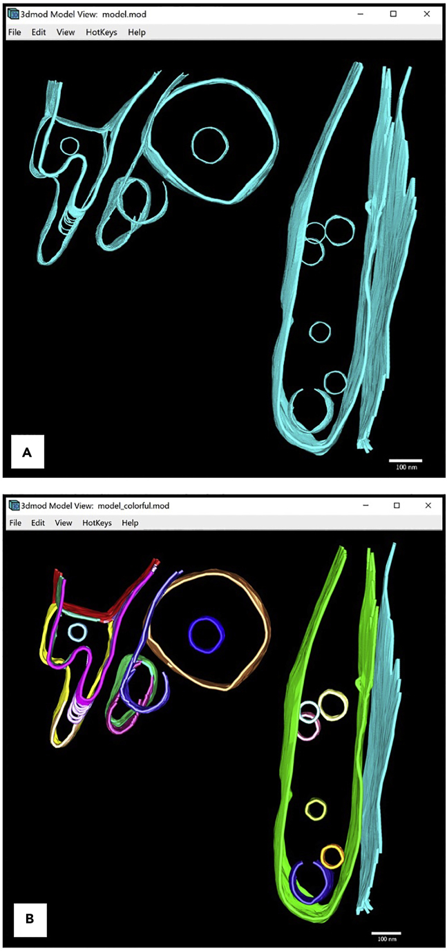
Continue until all the inner membranes and vesicles are annotated. See Figure 16A for our completed annotation of the chosen membrane-like structure.
Note: What criterion do you use to create a new object?
Figure 13.
Model of the target membrane displayed in Model View Window
(A) Top view of the model.
(B) Model rotated ∼45° around the y-axis.
Figure 14.
Steps for meshing
(A) Location of “Meshing” menu in the Model View Edit Object Window.
(B) Location of “Tube” checkbox, “Diam” box and “Dome cap” checkbox in “Meshing” menu.
(C) Location of “Mesh One” button in “Meshing” menu.
(D) Target membrane after meshing displayed in Model View Window. Note: All locations are circled in red.
Figure 15.
Steps for coloring in Model View Edit Object Window
(A) Location of “Line Color” menu in the Model View Edit Object Window circled in red.
(B) Location of the color sliders in the “Line Color” menu of the Model View Object Editing Window circled in red.
(C) Model of the target membrane rotated ∼40° around the y-axis, colored in cyan, displayed in Model View Window.
Figure 16.
Annotations of all inner membranes and vesicles in the tomogram displayed in Model View Window
(A) All Objects colored in cyan.
(B) Multi-colored Objects.
For first-time users, we recommend creating a new Object for each instance of the structure being annotated. It is possible to have Contours of different instances under the same Object where interpolation could yield favorable results. However, depending on the tomogram, this method might yield undesired interpolated Contours. Therefore, we recommend having one instance only under each Object.
Another case when an annotator should consider creating new Objects is when a continuous membrane appears to have holes on some Z-slices. These could be actual fenestrations in the membrane or simply an artifact from tomographic reconstruction. We recommend either creating a new Object for each segment visible in the Z-slices where holes are present or creating a new Object for one side of it, while annotating the other side as part of the Object that contains the annotations of the membrane when it is still continuous. These decisions are left at the discretion of the annotator.
An example where we created several Objects for the same inner membrane is the irregular looking membrane in the top left corner of the model shown above. Figure 16B below shows the same annotation where each Object is given a different color to show the number of objects for each membrane.
An Object needs to be created for every instance of structure that is continuous; in our example above, that would be for every continuous section of an inner membrane. We need to adhere to this rule in order to be able to successfully interpolate on our manually drawn Contours. If the Object contains manually drawn Contours of several inner membranes/vesicles, when we try to interpolate, weird intermediate lines might appear, or the program might even refuse to interpolate.
Sometimes it also happens that we have a continuous membrane, and then in some slices, somewhere in the middle, a section of the membrane disappears. In that case, we can annotate one side of it as part of the same Object and create a new Objects for the other side; creating two new Objects for each of the sides should work too.
The model can be saved either by pressing the S key on your keyboard or by navigating to File and pressing Save Model in the Information Window, and you are free to exit IMOD.
Segmentation
Timing: <5 min
At this point, you should have all the inner membranes and vesicles annotated and denoted by their respective Object number. In this step, we will group all the inner membranes together and ultimately create a single file with all inner membranes annotations, and no other structures. We will then use this file to extract the annotated features from the tomogram; that is, to produce a segmentation, which is real data from the regions that were annotated. All the actions that follow will be executed from the terminal unless otherwise stated.
-
22.First, we will need to create a mask according to the annotations of the membranes using the IMOD function imodmop. This command will draw a tube around each contour of all the Objects called upon of a given diameter. Type a command similar to the following one in the terminal:>imodmop -tube x -diam y -pl model_file.mod tomogram_file.mrc output_file.mrc
-
a.x is a list of open Contour Objects for which a tube will be drawn around each Contour (e.g., -tube 3 -tube 1–20 or -tube 1, 3, 5).
-
b.y is the diameter of the tubes to be drawn that we chose when we were meshing, which for membrane-like structures in this example should be 8 as decided earlier.
-
c.-pl, or -planar, instead of a 3D tube around each Contour, this ensures that the tube drawn is drawn in 2D, exclusively on the slice where the Contour is, without bleeding onto any other slices above or below.
-
d.model_file.mod is the file where the model with the IMOD annotations was saved.
-
e.tomogram_file.mrc is the original file with the 3D image that we were annotating.
-
f.output_file.mrc is the file that the command will output. We recommend that the file name contains the name of the structure being annotated (e.g., tomogram_structure.mrc).Note: Make sure that all the Objects of the same type are in the same file. The way that you group the Objects is entirely up to you; you can group together all inner membranes by specifying the numbers of all the Objects that contain them after -tube in the imodmop command above, for example, or you can call imodmop on each one of them separately. The difference will be that you will be able to manipulate the Objects from the same file together, while on the other hand you can have different settings for Objects in different files.
-
a.
-
23.
As the last step, if the tomogram you are working with has “negative contrast” (which means that the densest biological features of the tomogram appear in black or darker tones, see figure below for reference), use a command similar to the one below to invert the contrast, just making sure that your input file name corresponds to the tomogram you’re working on (note that you can pick any name you like for the output; here, we just add “_inv” as a tag that tells us the output has been “inverted” or “contrast-reversed”):
>clip contrast -n -1 tomogram_structure_all.mrc tomogram_structure_all_inv.mrc
-
24.
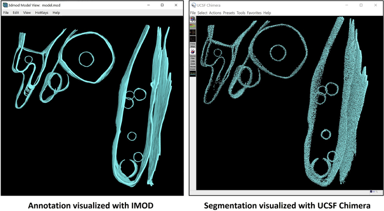
The resulting annotation and segmentation should look similar to the ones in Figure 17.
Optional: Other useful IMOD commands.
Figure 17.
Annotation (displayed in ZaP Window, left) and segmentation (displayed in UCSF Chimera, right) of all the inner membranes and vesicles of the tomogram
If you have already created a file with a subgroup of the inner membranes, and later you altered the model file to contain more Objects with inner membranes, you can update the segmentation file to contain the previously annotated inner membranes as well as the new ones. To do this, use the imodmop command above only on the newly created Objects that represent inner membranes, then merge the two (or more) segmentation files that were output by imodmop with a command like the following:
>clip add tomogram_segmentation_1.mrc tomogram_segmentation_2.mrc tomogram_segmentation_3.mrc … tomogram_segmentation_all.mrc
where all files are inputs, except for the last one which is the target output file that will contain all input files merged.
If you have some annotated structures in one model, and some in another model, and you want to merge the two models together, you can use the following command:
>imodjoin model_1.mod model_2.mod output_model.mod
At this point we have finished segmenting all the membrane-like structures from the example tomogram, and we can open the file tomogram_structure_segmentation.mrc using UCSF Chimera to visualize the result.
Annotating globular structures
This method is for annotating and segmenting large globular structures, such as lipid droplets, mitochondrial granules, cytoplasmic stress granules, virions infecting cells, etc.; literally anything with a globular shape. The annotation will delineate the boundary of the structure as well as its insides. For example, in this protocol, I will use this method to annotate intracellular lipid droplets. As before, each instance of the structure will be its own Object.
Setting up
Timing: 5 min
This section will guide the User to properly set up all the IMOD windows that will be used during annotation.
-
25.
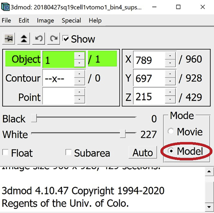
In the Information Window make sure that Model is selected.
-
26.
In Edit Object Window choose Object Type Closed. In Edit Object Window check the box next to Start new Contour at new Z. Also in Edit Object Window, choose a name for the Object and write it in the area under Object name (e.g., Lipid droplet 1).
-
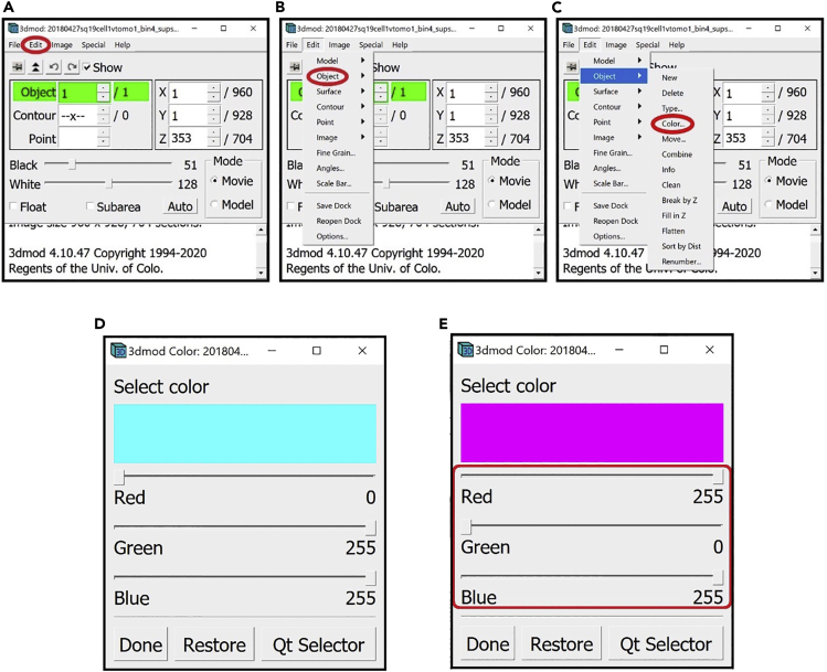
27.We can change the color of the Object, for example to magenta.
Figure 18.
Instructions for changing the color of the currently selected Object from Information Window
(A) Location of the “Edit” drop-down menu in the Information Window.
(B) Location of the “Object” drop-down menu in the “Edit” drop-down menu.
(C) Location of the “Color…” button in the “Object” drop-down menu.
(D) Window for changing the color of the currently selected Object set to cyan.
(E) Window for changing the color of the currently selected Object set to magenta. Note: All locations are circled in red.
Manual annotation
Timing: < 30 min
The manual annotation step for globular structures is very similar to the manual annotation for membrane-like structures. We will still be adding contours at every 4th-10th Z-slice; however, now it will be on the boundary of the structure, as opposed to the middle of the membrane.
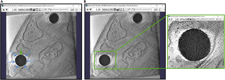
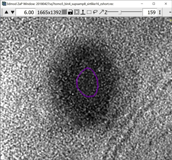
The target structure in this case is the lipid droplet pointed to by the blue arrows in the image below (Figure 19A). We will start the annotation at the point indicated by the green arrow (Figure 19A) and our objective is simply to roughly encircle the feature. You can make your Contours as smooth or rugged as desired.
-
28.
We will again zoom in to the lipid droplet to annotate it more accurately. Remember how when annotating the membrane, we had to navigate between four regions to be able to annotate the entire membrane (Figure 5).
Figure 19.
Target vesicle-like structure on z-slice 225 of a tomogram
(A) The blue arrows point to the target structure. The green arrow indicates the start point of the Contour.
(B) ZaP Window displaying a slice of the tomogram containing the target vesicle-like structure, with the region of the target structure boxed out in green, and a zoomed-in version of the region.
The lipid droplet is much smaller than the membrane, so one zoomed-in region can contain the entire lipid droplet. Zoom in by a factor of 6.0× around the lipid droplet, as shown in Figure 19B.
-
29.
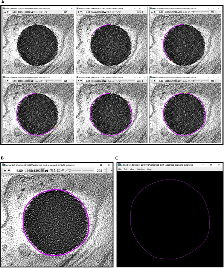
Create a Contour just outside the boundary of the lipid droplet. As before, you can use Middle Click, Right Click and Backspace to add Points (Figure 20A).
-
30.
The resulting Contour should look like this in ZaP Window (Figure 20B) and Model View Window (Figure 20C).
Optional: Another, easy way to create circular Contours is to use other Drawing Tools from the Drawing Tools Window, especially Sculpt and Warp.

Figure 20.
Creating a Contour for the target vesicle-like structure
(A) Steps for creating a Contour of the target structure at z-slice 225 using “Normal” Drawing mode displayed in ZaP Window.
(B) Completed Contour of the target vesicle-like structure displayed in ZaP Window.
(C) Completed Contour of the target vesicle-like structure displayed in Model View Window.
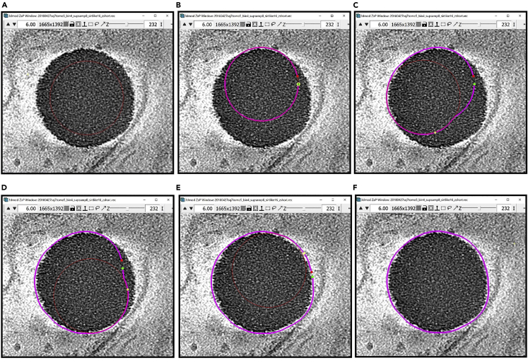
You can select a different Drawing Tool by either opening the Drawing Tools Window and selecting, or by pressing the corresponding number key on your keyboard when in ZaP Window (such as 2 for Warp or 3 for Sculpt). When you select either Drawing Tool, a circle appears around the mouse; you can change the size of this circle with the use of the Scroll Wheel on your mouse.
Open the ZaP Window and Zoom in to the lipid droplet. Select the Sculpt Drawing Tool. Increase the size of the circle to be a bit smaller than the lipid droplet (Figure 21A).
Figure 21.
Creating a Contour for the target vesicle-like structure using “Sculpt” Drawing Tool
(A) ZaP Window displaying the target vesicle-like structure with the “Sculpt” Drawing Tool appearing as a red circle inside the target structure.
(B–E) Steps for creating a Contour of the target vesicle-like structure using “Sculpt” Drawing Tool.
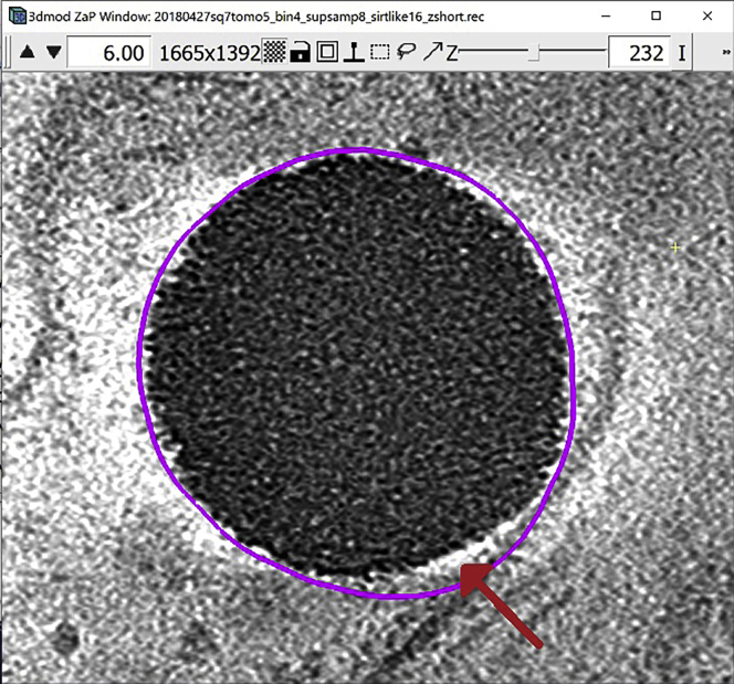
(F) Completed contour of the target vesicle-like structure at z-slice 232, created using the “Sculpt” Drawing Tool, displayed in ZaP Window.
Middle Click and hold while moving the circle along the boundary of the lipid droplet (Figures 21B–21E).
The result could look similar to Figure 21F.
The contour above encloses the entire lipid droplet; therefore, we can say that this is a sufficiently good Contour. In the case that the Contour is not sufficiently accurate, you might want to use the “Warp” Drawing Tool as described in Troubleshooting 1.
Note: Normal vs. Sculpt + Warp.
As mentioned before, the advantage of using the Normal drawing mode over Sculpt+Warp for annotation is that the former creates Contours with fewer Points. Even though annotations will vary depending on the annotator and the structure being annotated (Hecksel et al., 2016), and thus the number of Points per Contour is expected to vary, Sculpt+Warp will tend to produce Contours with more Points. For example, we annotated the lipid droplet above by using both the Normal and Sculpt+Warp methods and recorded the number of Points per Contour in Table 1. Notice that the average number of Points per Contour is 37.8 for Normal and 136.1 for Sculpt+Warp; therefore, the number of Points increased by a factor of 3.6× on average when using Sculpt+Warp to annotate this structure.
Table 1.
Table showing the difference in the number of Points per Contour between the “Normal” and the “Sculpt+Warp” method of creating Contours
| Maximum no. of points/Contours | Minimum no. of points/Contours | Average no. of points/Contours | Standard deviation | |
|---|---|---|---|---|
| Normal | 71 | 19 | 37.8 | 18.2 |
| Sculpt+Warp | 218 | 63 | 136.1 | 57.5 |
The table contains the maximum, minimum, and average number of Points per Contour, as well as the standard deviation.
The only potential problem we have identified with the Sculpt+Warp method is that IMOD may lag on a computer with modest specs when the size of the Model file is large, and the size of the file will depend on the number of Objects, Contours, and Points it contains. Below is an IMOD command that can decrease the number of Points in a Contour without compromising the annotation results. You can use it if you prefer the Sculpt+Warp method but might notice that IMOD may lag. First save your model and close IMOD. Then type a command similar to the following at the terminal:
>reducecont input_file.mod output_file.mod
Make sure to provide the correct file name for the input, and you may choose any name you want for the output. Re-open IMOD with the newly created model and notice the change in the number of Points for the Contours. For perspective, some manual annotations of this same specimen contained 23002 Points originally and this number was reduced to 6936 using the command above. The table below (Table 2) contains the maximum, minimum, average and standard deviation of the number of Points per Contour using the Normal vs Sculpt+Warp methods, together with a third method: Sculpt+Warp+Reducecont. Notice that the average number of Points per Contour for Sculpt + Warp + Reducecont is very close to the average number of Points per Contour for the Normal method: 41.041 and 37.766, respectively. Therefore, both methods achieve extremely similar results, and you can choose whichever method is more suitable for your structure and more efficient for you as an annotator.
-
31.
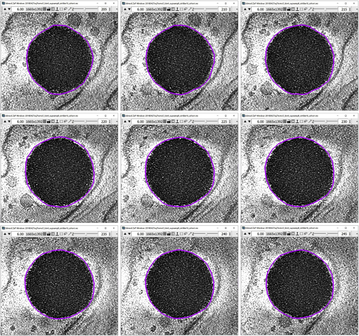
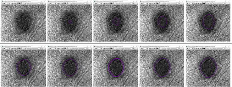
After finishing one Contour with one of the methods mentioned above, continue adding Contours at other slices. I chose to add one Contour over five slices. Starting from 225, add a Contour at 220, 215, 210, so on and so forth, and in the other direction, at 230, 235, 240, etc. The figure below shows nine Contours: at 225, and four other Contours above and below the 225 Z-slice:
Table 2.
Table showing the difference in the number of Points per Contour between the “Normal,” “Sculpt+Warp” and “Sculpt+Warp+Reducecont” method of creating Contours
| Maximum no. of points/Contours | Minimum no. of points/Contours | Average no. of points/Contours | Standard deviation | |
|---|---|---|---|---|
| Normal | 71 | 19 | 37.8 | 18.2 |
| Sculpt+Warp | 218 | 63 | 136.1 | 57.5 |
| Sculpt+Warp+Reducecont | 49 | 17 | 41 | 5.8 |
The table contains the maximum, minimum, and average number of Points per Contour, as well as the standard deviation.
For this lipid droplet, we added 24 Contours, from Z-slice 170 through 285, in steps of five slices.
Note: A problem arises at the top and the bottom Z-slices of the lipid droplet, where the boundary of the droplet cannot be seen as clearly due to the “missing wedge,” which causes anisotropic resolution in all limited-angle tomography reconstructions (Radermacher, 1988), and drawing the Contours at those slices would be more similar to guessing than to annotating the boundary (the panels below show examples of slices through a large lipid droplet where the edge is clear, as in the left-hand-side panel, vs slices where the edge is more fuzzy, as in the middle panel, or indistinguishable, as in the right-hand-side panel). For the Z-slices in which the object of interest has indistinguishable or ambiguous edges, we believe that the most intellectually honest approach is simply to omit the Contours. However, Users are free to annotate as many or as few Z-slices as desired depending on the purposes of their annotations and the confidence level in delineating the boundaries.
-
32.
Navigate to the Model View Window and you can see in 3D the lines of the Contours that you traced (Figure 22).
Figure 22.
Manually drawn Contours of the target vesicle-like structure displayed in Model View Window
(A) Top view of the model.
(B) Model rotated ∼45° around the y-axis.
Interpolation
Timing: < 30 min
This section will guide the User to interpolate approximately spherical structures.
-
33.
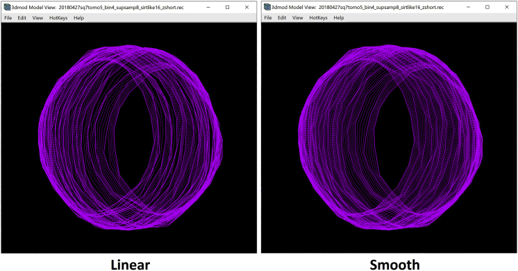
For the interpolation step, you can again choose either Linear or Smooth interpolation. Both methods will yield all the missing Contours between the manually drawn Contours, therefore the resulting shape will be a spheroidal shell with two poles cut off. The panels below show side-by-side the results from using the two interpolation methods.
-
34.
In this case, Smooth interpolation yields a noticeably smoother surface than Linear interpolation, and it predicts the missing Contours better. Therefore, if we had to choose between the two types, we should choose the Smooth interpolation for this type of feature.
-
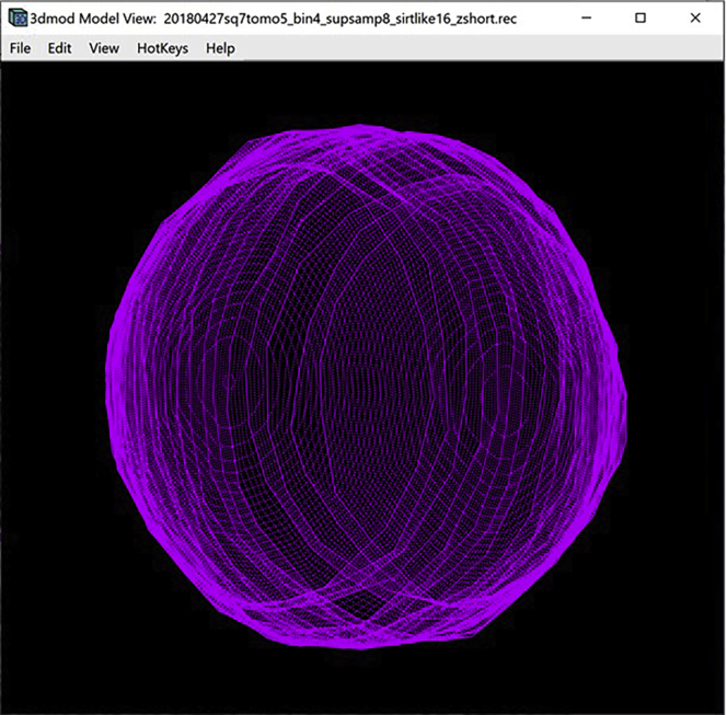
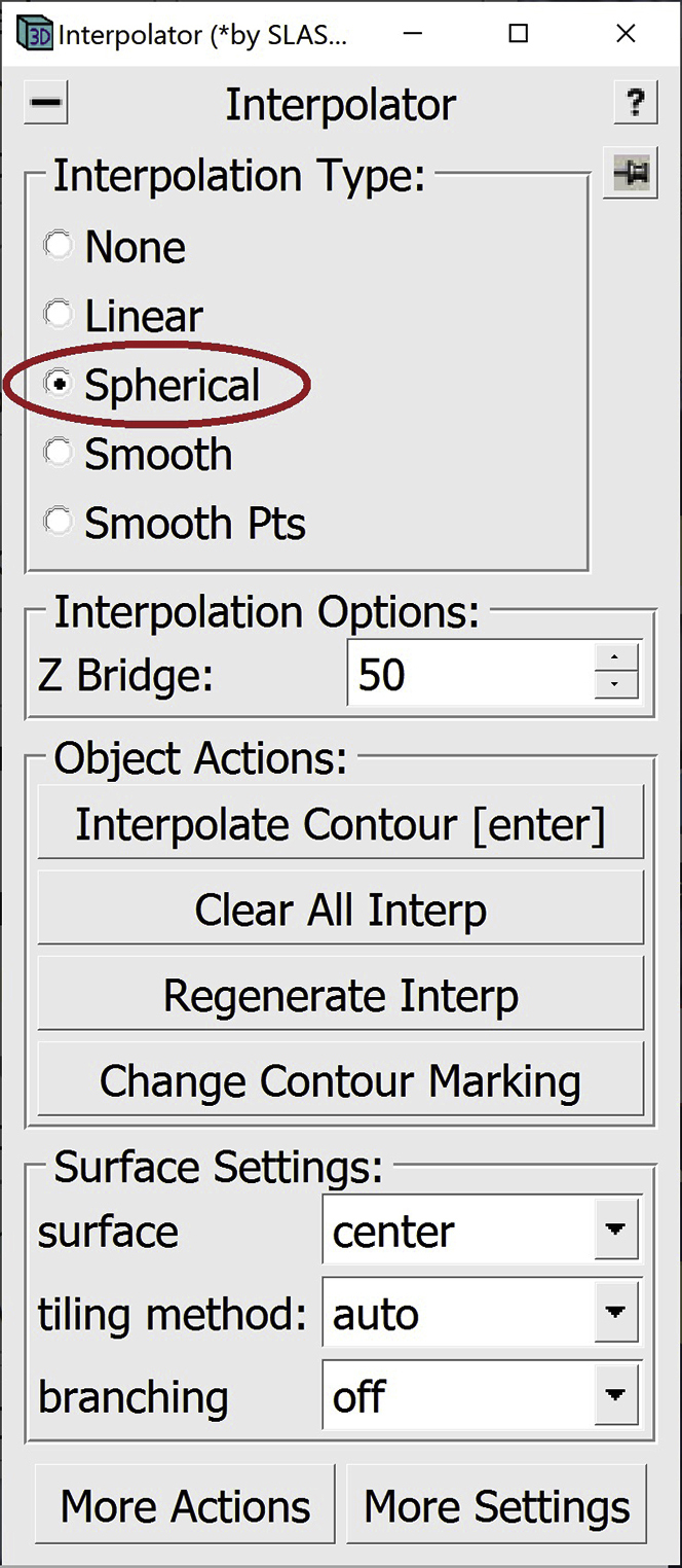
35.Another interpolation method that can be used for globular structures is Spherical interpolation.
-
a.You can select the Spherical interpolation type in the Interpolator Window.
-
b.When called on one Contour, Spherical interpolation adds all the Contours in between the manually drawn Contours, just like Smooth interpolation. However, it also approximates the two poles that are missing in the two interpolation methods described above (see below). This may be appropriate for didactic purposes, or if we already know, a priori, that the true shape of the feature of interest is indeed spheroidal, and the missing wedge artifact is not “hiding” something unique in that region.
-
a.
-
36.After the interpolations are drawn, you should check that all of them approximate the boundary well enough. For the intermediate Contours between the manually drawn Contours, correct the Contours as done for the interpolations of the membrane-like feature in the first section of the Protocol.
-
a.If you choose to use Spherical interpolation, check the top and bottom Contours carefully. You will notice that sometimes the approximation closes the sphere too soon or too late. For example, the figure below shows an interpolated Contour that seems to close the sphere too soon.
-
b.In this case, you can choose a Z-slice somewhere in the middle between the Z-slice with your last manually drawn Contour, and the Z-slice where you think you cannot see the lipid droplet anymore. The chosen Z-slice should be one where the Contour is inaccurate and on which you think you can draw a better Contour. In this case, we will choose the slice immediately above the one where it is apparent that the spherical interpolation closed “too early”.
-
c.Delete the Contour by selecting it with Left Click and then typing Shift+D. Now, draw the Contour manually and, upon finishing, press Enter to interpolate again. Repeat this process again and again, moving farther each time from the “equator” of the lipid droplet, until you think that the interpolations are good enough. Usually, you would not need to do this more than three times. The figure below shows an example of several slices around Z-slice 159 before and after doing the process above only once at Z-slice 159.
-
a.
Meshing and 3D visualization
Timing: <5 min/Object
This section will describe the meshing step for solid (filled) globular structures, which is very straightforward.
-
37.
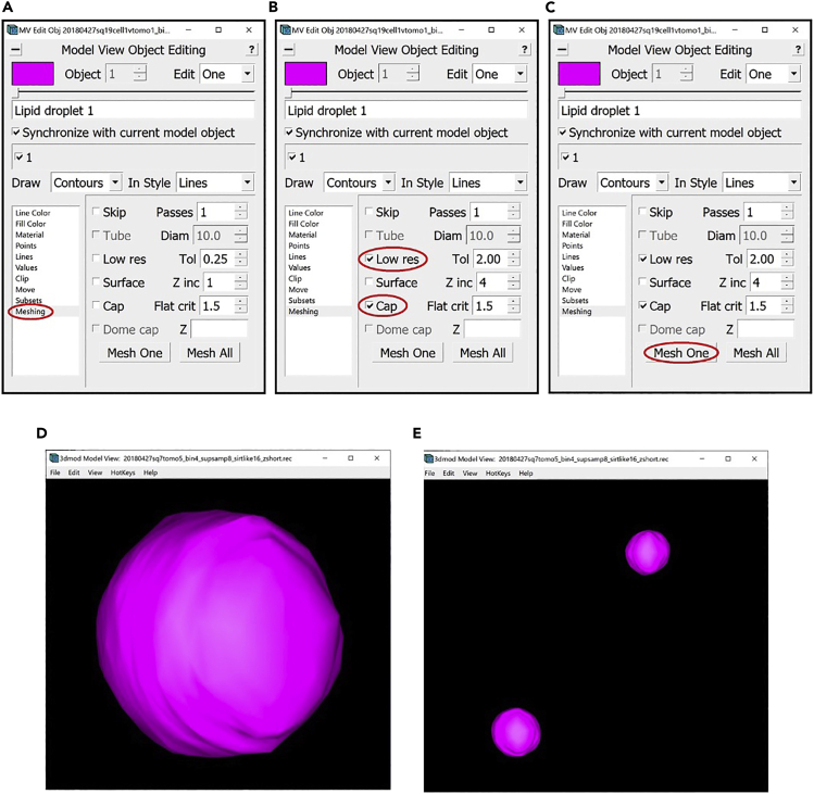
Open the Model View Window and the Model View Object Editing Window. In the Model View Object Editing Window, in the menu on the left, select Meshing (Figure 23A). For globular structures, in the Model View Object Editing Window, check the box next to Cap and the box next to Low res (Figure 23B). Now press the Mesh One button and see the results in the Model View Window (Figure 23C).
-
38.
View the meshed membrane in the Model View Window (Figure 23D).
-
39.
The annotation for this lipid droplet is now complete. Repeat the process until all the lipid droplets in the tomogram are annotated. Since the tomogram has only two lipid droplets, the result looks similar to Figure 23E.
Figure 23.
Instructions for meshing the target vesicle-like structure
(A) Location of the “Meshing” menu in the Model View Object Editing Window.
(B) Location of the “Low res” and “Cap” checkboxes in the “Meshing” menu.
(C) Location of the “Mesh One” button in the “Meshing” menu.
(D) Model of the target vesicle-like structure after meshing displayed in Model View Window.
(E) Completed annotation of all lipid droplets in the tomogram displayed in Model View Window. Note: All locations are circled in red.
Segmentation
Timing: <5 min
This section will provide the steps for creating a segmentation of the desired structure. All the actions that follow will be executed from the terminal unless otherwise stated.
-
40.First, we will use imodmop, which will draw inside the meshed region. Type a command similar to the following in the terminal:>imodmop -objects x (-pad y) model_file.mod tomogram_file.mrc output_file.mrc
-
a.x is a list of closed Contour Objects for which the inside areas will be drawn (e.g., –objects 3 -objects 1–20 or -objects 1, 3, 5).
-
b.-pad y is optional; you can add this in case you think that your Contours might not be very accurate and that part of the lipid droplet might not be inside the Contour; this command adds a padding of size y (in pixels), which could be a value between 1 and 3 (for example), to the outside of the Contour, thereby including the areas that might be outside of the Contour.
-
c.model_file.mod is the file where the model with the IMOD annotations was saved.
-
d.tomogram_file.mrc is the original file with the 3D image being annotated.
-
e.output_file.mrc is the file that the command will output. We recommend that the file name contains a string to identify the structure being annotated (e.g., tomogram_structure.mrc).
-
a.
-
41.
As the last step, if the tomogram you are working with has negative contrast, use the command below to invert the contrast:
>clip contrast -n -1 tomogram_structure.mrc tomogram_structure_inv.mrc
At this point we have finished segmenting all the lipid droplets from the given tomogram, and we can open the file tomogram_structure_inv.mrc using any appropriate visualization software.
Annotating tubular/filamentous structures
This section will focus on annotating and segmenting tubular structures. The annotation method will be very similar to the method used for annotating membrane-like structures, in the sense that the Contours drawn have to be in “the middle” of the target structure. The difference, however, is that tubular structures typically occupy only a few Z-slices but undulate through the “depth” of the tomogram, thus making following them more challenging than large, continuous membranes. Therefore, this method will explain how to create Contours that go across Z-slices at oblique angles (sometimes twisting and/or turning) in order to annotate tubular structures.
Setting up
Timing: 2 min
This section will guide the User to properly set up all the IMOD windows that will be used during annotation.
-
42.
In the Information Window make sure that Model is selected.
-
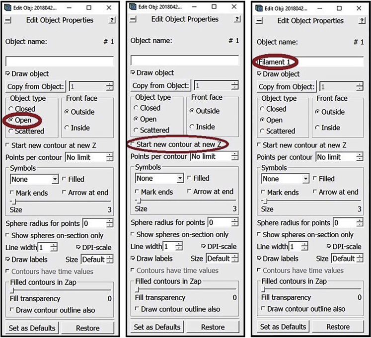
43.
In the Edit Object Window, choose as Object Type Open. In the Edit Object Window, uncheck the box next to Start new contour at new Z. Also in the Edit Object Window, choose a name for the Object and write it in the area under Object name (e.g., Filament 1).
Manual annotation
Timing: < 15 min/instance
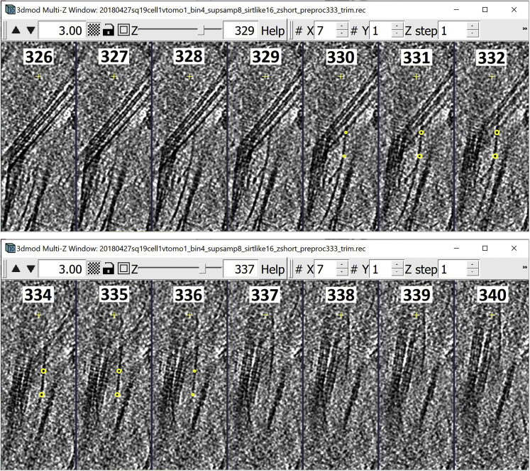
In the manual annotation step we will add Contours that span multiple Z-slices in order to create annotations of tubular structures in 3D that are not fully contained in any single XY plane or Z-slice, but rather their positions vary as they undulate/curve/bend in multiple directions.
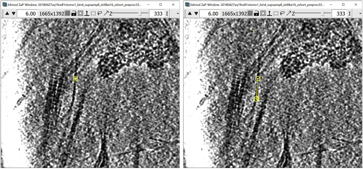
The first target feature is the filament pointed to by the blue arrow in Figure 24.
-
44.
Zoom in to the filament as shown in Figure 24.
-
45.Before we start annotating, we need to find the diameter of the filament.
-
a.Choose a region of the structure where it appears the darkest and add three points.
-
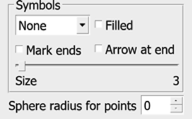
b.Open Edit Object Window and find the settings below.
-
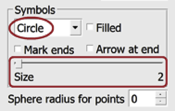
c.From the drop-down menu under “Symbols”, select Circle. Then move the Size slide bar to 2.
-
d.The Contour should now look similar to the figure below.
-
e.Use the arrows next to Sphere radius for points to draw a sphere of a given radius around each Point and see which radius provides circles that can cover the entire diameter of the structure. For example, below are images of the ZaP Window where the Sphere radius for points was set to 3 (panel A below) and 4 (panel B below) pixels, respectively.
-
f.A radius of 3 pixels seems to cover well enough the entire diameter of the filament, however we want it to be slightly wider than the actual diameter of the structure to make sure that if we turn this annotation into a mask to produce a segmentation, the densities of the feature will be fully captured within the mask; therefore, we will use a radius of 4 pixels.
-
g.After finding the thickness of the target structure, do not change the settings in this window. The Edit Object Window should stay with the previous settings.
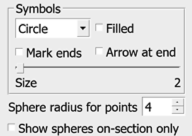
-
h.Now, delete the three points you added, leaving the Object with no Contours.
-
a.
-
46.In the ZaP Window, we can move up and down the Z-slices to see how the filament curves upwards as we go further from the cell’s outer membrane. Starting at Z-slice 333, the figure below shows the filaments in other Z-slices above (left) and below (right).To annotate a tubular structure requiring Contours that are not circumscribed to an XY plane or Z-slice, we will need to work on several Z-slices concurrently. We can do that by using IMOD’s feature Multi-Z, where we can open several Z-slice and annotate them.
-
a.To open the Multi-Z Window, in the Information Window, select Image in the menu at the top of the window. In the drop-down menu, click on Multi-Z.
-
b.The Multi-Z Window will appear on the screen (Figure 25A).
-
c.Right Click and hold while dragging the mouse to move to the region where the target feature is visible (Figure 25B).
-
d.You can manipulate how many slices you see by changing the #X and #Y at the top of the window. #X represents the number of slices per row, and #Y represents the number of rows. So, if we increase #X to 6 and #Y to 2 you will see something similar to Figure 25C.
-
e.Then you can change the size of the window itself to visualize larger regions (Figure 25D).
-
f.This example was annotated with #X set to 7 and #Y to 1, modifying the “zoom” level (top left arrows) and resizing the window as needed (Figure 25E).
-
g.Although we will still be annotating in the ZaP Window, the Multi-Z Window can help us check that the annotation is following the structure across the Z-slices accurately. Therefore, for the next steps, keep both the ZaP and Multi-Z Windows open.Optional: For easier visualization, you can change the color of the Object (in this case, we changed it to yellow).
-
a.
-
47.
We choose a slice where we can see a segment of the structure very clearly; the segment should be small, continuous, and very dark. The segment does not have to be right at the edge of the structure. You can trace the structure through the Z-slices to a slice that has a certain region that you are confident annotating (maybe in the middle of filament). Usually the start and the end of the filament are more difficult to see and annotate, either because they’re merging with other structures (the membrane) or getting progressively thinner (toward the tip) and are thus less dense and more obscured by the high noise levels, so try to start at a region where you are confident that you can see and trace the structure (for example, see Figure 26A).
-
48.
Check the Multi-ZaP Window to ensure that the current slice is showing the target segment to annotate at its darkest or “densest” part. (Note that the Z-slice number displayed in the menu bar at the top of the window refers to the Z-slice that appears in the middle of the Multi-Z Window. For example, in Figure 26B, the 333rd slice is the slice indicated by the blue rectangle).
Figure 24.
ZaP Window displaying a slice of the tomogram containing the target tubular structure, in the region boxed out in green, and a 4× zoomed-in view (right)
Figure 25.
Instructions for setting up the Multi-Z Window
(A) Multi-Z Window upon opening.
(B) Multi-Z Window displaying the region with the target structure.
(C) Multi-Z Window with #X of 6 and #Y of 2.
(D) Re-sized Multi-Z Window.
(E) Re-sized Multi-Z Window with #X of 7 and #Y of 1.
Figure 26.
Using ZaP Window for annotation of target tubular structure
(A) ZaP Window displaying the target structure at Z-slice 333, with a yellow segment showing the densest region of the structure.
(B) Multi-Z Window displaying the target tubular structure, with Z-slice 333 denoted by the blue rectangle, and a yellow segment showing the densest part of the filament at slice 333 on every slice.
(C) ZaP Window displaying the target structure at Z-slice 333 with one Point added.
(D) Multi-Z Window displaying the target structure with one Point added at Z-slice 333.
(E) Multi-Z Windows displaying the target structure at Z-slices below (top Window) and above (bottom Window) Z-slice 333.
The two slices right above and below the Z-slice 333 show the segment we’re starting the annotation with similarly good contrast; however, we can see that in the furthest slices, the segment starts to fade off at the ends. This means that if we add a Point in the middle of the filament at the current Z-slice on the selected segment, we will have a point in the center of the tubular structure (in Z), and if we create a tube around that Point (in 3D), it should enclose the entire width of the structure in Z.
-
49.
In the ZaP Window, add a Point somewhere on the segment (Figure 26C). Then, look at the Multi-Z Window (Figure 26D). You will notice that since we are drawing a sphere around each Point, the current Z-slice will have a yellow circle around the Point of a certain radius (4 pixels in this case) and the circles around the same Point at adjacent slices will be smaller as we go further away from the current Z-slice, like cross-sections through a sphere in 3D.
-
50.
Go up and down the Z-slices and analyze the slices right above and below the smallest circle that closes the sphere (Figure 26E).
If we look at the Z-slices below slice 330, which is the Z-slice where the yellow sphere closes at the “bottom”, we can see that the filament becomes dimmer as we go down the Z-slices, completely disappearing at Z-slice 326. We want to see the same trend at the other end as well. At the “top”, the last cross-section circle of the yellow sphere around the added Point is on slide 336, and the filament slowly dims out from there on, completely disappearing on slice 240. Seeing this we can conclude that the point that we added is roughly at the center of the tubular structure in Z.
Note: We might question whether the radius is big enough. If we indeed wanted to enclose the entire structure, we might want to increase the sphere radius so that the last circle appears on the slice where we can see the last traces of that Point on the structure. However, because of the missing wedge, densities in 3D tomograms appear elongated in the direction of the Z-axis (due to anisotropic resolution that lowers the resolution in Z). You may try to compensate for this by leaving a few slices of the feature unannotated in Z at either end, under the assumption that the structure is indeed cylindrical. Alternatively, you may add more Points to annotate the feature in all Z-slices where you can see it, knowing that the true thickness of a tubular filament only appears unaltered by the missing wedge in XY planes. Either way, here we advise that you start the annotation in the “center” making sure that the segment disappears on both sides at the same rate, for example on slices 327 and 339 we can barely see the segment, and on slices 326 and 340 it completely disappears.
-
51.Continue adding Points along the filament using the same method:
-
a.Choose a small segment where you want to add a Point.
-
b.Check in the Multi-Z Window that the Z-slice at which you want to add the Point corresponds to the darkest/densest part of the segment compared to the adjacent Z-slices.
-
c.Place the Point.
-
d.Check the Z-slices above and below to see that the segment disappears at the same rate at both ends.
-
a.
-
52.
Since we chose an arbitrary segment to add the first Point, we will probably have more densities to annotate on the same structure both “upwards” and “downwards” along the filament axis (Figure 27A).
Figure 27.
Understanding direction of annotation of tubular structure
(A) ZaP Window displaying the target structure at Z-slice 333 with the first Point added, and the orange arrow showing the “upward” direction and the yellow arrow showing the “downward” direction in the slice.
(B) ZaP Window displaying the target structure at Z-slice 328 after Points have been added along the structure in the “downward” direction.
(C) ZaP Window displaying the target structure at Z-slice 333, with the orange arrow showing the “upward” direction.
Choose one direction to annotate first. In this example, we will annotate “downward” first to then return to the first Point and continue annotating “upwards”.
- 53.
-
54.
As mentioned before, you should add Points at a small distance from each other – the smaller the distance, the better the accuracy of the annotation. Be aware that this method might require a lot of trial and error; however, the results will offer an amazing 3D visualization of the tubular structures you are annotating.
-
55.
Continue adding Points downwards along the filament until you reach the end of the structure and/or the boundary of the tomogram (Figure 27B).
-
56.When you have finished annotating downwards, you have to return to your first Point and annotate upward (Figure 27C).
-
a.Select the first Point you created. If we add a Point using Middle Click above this Point, the newly created point will become Point 2, while all the Points below the first Point will increase by 1, with the old Point 2 becoming Point 3, the old Point 3 becoming Point 4, so on and so forth. Hence, the Contour will start at the first Point you created, then will go above Point 1, then to the point below Point 1. To understand this better, you can add a new Point to the side of the filament you are annotating, which will exaggerate the Contour line (Figure 28A).
-
b.Notice how the new Point creates a sharp kink to the side. This happens because the new Point is not in the “right order”, continuous with the numbering of the prior Points in the Contour (strictly increasing in one direction and decreasing in the other). To ensure that the Points are added in the correct order, we need to “invert” the Contour before annotating upwards from the first Point.
- c.
-
d.Notice how the green circle changed to a red circle in the ZaP Window.
-
e.Now if we add a Point above the first one to the side of the filament as before, the Contour will create a line with the new Point at the end of the Contour, instead of having the new Point be in “the middle” of the Contour (Figure 28E).
-
a.
-
57.
The resulting Contour should look like the one in Figure 29A in the Multi-Z Window with #X and #Y adjusted to see all slices containing Points in the Contour.
-
58.
In Model View we can see the Contour in 3D. The figure below shows the model in the XY plane (Figure 29B) and in the YZ plane (Figure 29C).
-
59.
Having one filament fully annotated, we can proceed to annotate the rest. However, one difference between annotating tubular/filamentous structures and the other two types of structures covered before, is that here we do not need an Object per instance (that is, for each filament). For example, above we have one Object with one Contour for the first annotated filament; we can continue adding Contours to the same Object to annotate other instances. So, in this case, instead of having one Object per instance, we can have one Contour per instance, all Contours being under the same Object. The reason why we had to create distinct Objects for each instance of a structure in the globules and membranes examples was that we had to interpolate Contours at the Z-slices that we skipped. Here, there is no need for interpolation, since one Contour covers the entirety of one structure if the diameter of the sphere is set to the appropriate width to cover the thickness of the filament. Therefore, we can have one Object containing all the filaments.
-
60.For the example here we annotated all the filament with a diameter of 8 (or radius 4) under a single Object (Figure 29D).Note: On the other hand, there may be reasons why we might want to separate the filaments into different Objects:
-
a.If there are different types of tubular structures in the tomogram, and we want to color them differently when visualizing the model.
-
b.If all the tubular structures are of the same “type”, but they vary in diameter. For this we would want to have several Objects, each with its own diameter class for the tubes that we mesh later.
-
a.
Figure 28.
Inverting contour
(A) ZaP Window displaying the Contour of the target structure, with a new Point added above and to the side of the first Point, with a zoomed-in image shown in the blue rectangle.
(B) Location of the “Edit” drop-down menu in the Information Window.
(C) Location of the “Contour” drop-down menu in the “Edit” drop-down menu.
(D) Location of the “Invert” button in the “Contour” drop-down menu.
(E) ZaP Window displaying the Contour of the target structure, with a new Point added above and to the side of the first Point, with a zoomed-in image shown in the blue rectangle. Note: All locations are circled in red.
Figure 29.
Meshing the model of the target tubular structure
(A) Re-sized Multi-Z Window with adjusted #X and #Y to show the entire Contour of the target structure.
(B) XY plane view of the model of the target tubular structure displayed in the Model View Window.
(C) YZ plane view of the model of the target tubular structure displayed in the Model View Window.
(D) Model containing all filaments in the tomogram displayed in the Model View Window.
Meshing and 3D visualization
Timing: ∼5 min
This section provides steps to create a 3D image from an annotated model.
-
61.
Open the Model View Window and the Model View Object Editing Window. In the Model View Object Editing Window, in the menu on the left, select Meshing as shown in the left-side panel below. For tubular structures, in the Model View Object Editing Window, check the box next to Tube and change the value of Diam to twice the “radius” that we found before, which in this case is 8, as shown in the middle panel below. Check the box next to Dome Cap. Now, press the Mesh One button, is shown un the right-side panel below.
-
62.
View the meshed filament in the Model View Window (Figure 30).
Figure 30.
Annotation of all filaments in the tomogram displayed in the Model View Window
Segmentation
Timing: ∼5 min
This section will provide the steps for creating a segmentation of the desired structure. All the actions that follow will be executed from the terminal unless otherwise stated.
-
63.First, we will use imodmop to create a mask according to the annotations of the membranes. The command below will draw a tube around each Contour of all the Objects called upon:>imodmop -tube x -diam y model_file.mod tomogram_file.mrc output_file.mrc
-
a.x is the number of the open Contour Objects that contain all the tubular structures (e.g., -tube 1).
-
b.y is the diameter of the tubes to be drawn that we chose when we were meshing, which for the example annotation above was 8.
-
c.model_file.mod is the file where the model with the IMOD annotations were saved.
-
d.tomogram_file.mrc is the original file with the 3D image that we were annotating.
-
e.output_file.mrc is the file that the command will output. We recommend that the file name contains the name of the structure being annotated (e.g., tomogram_structure.mrc).Note: These are the variables to give imodmop if you have one Object with multiple Contours, each containing an instance of your tubular structure, and all the instances you annotated have the same diameter. If you have several Objects that contain similar structures but with different diameters, check Troubleshooting 3.
-
a.
-
64.
As the last step, if the tomogram you are working with has negative contrast, use a command in the form of the one below to invert the contrast:
>clip contrast -n -1 tomogram_structure_all.mrc tomogram_structure_all_inv.mrc
-
65.
At this point we have finished segmenting all the filament from the given tomogram, and we can open the file tomogram_structure_segmentation.hdf using Chimera to visualize the result.
Expected outcomes
The expected outcomes have been illustrated with multiple figures throughout each section of the protocol.
Limitations
Manual annotation is not suitable for features that are very small or thin, making it difficult to distinguish them from the background noise. Also, annotation of features composed of thousands of individual instances (e.g., thousands of ribosomes in the cytoplasm) would be unfeasible because it would be inhumanely tedious and take too long. Features with complex voids (e.g., trying to annotate cytoplasm without including the organelles and other subcellular features) are also challenging to annotate with this protocol, but may be feasible if the feature can be modeled as a collection of smaller, compartmentalized, vesicle-like subregions. Lastly, it is well known that manual annotation is subjective and varies from user to user, and this is an important limitation in all manual annotation strategies.
Troubleshooting
Problem 1
When annotating globular features, using the Sculpt Drawing Tool to draw a circular Contour may be inexact because while the feature may be approximately circular, there may be local distortions that deviate from circular morphology; thus, when drawing the Contour, we might move the circle too much toward the outside and get a result as shown below, where there’s a large area of background mistakenly encased within the Contour.
Notice that in the bottom right part of the lipid droplet, the Contour is too far from the boundary.
Potential solution
We can use the Warp Drawing Tool to help us correct it. To do this, select the Warp Drawing Tool; you can do this by pressing 2 on the keyboard. Place the center of the circle along the membrane at the Point that is approximately in the middle of the incorrect Contour segment. Middle Click and hold while moving the mouse toward the boundary of the lipid droplet, until the Contour looks as desired.
Problem 2
What to do if you added a Point at the wrong Z-slice?
Example with filamentous structures: Suppose we want to add a second Point along the filament on the same Z-slice as the first Point (333), as shown below.
If the filament is not parallel to the XY plane and curves in or out in Z, this second Point might not be at the “correct” Z-slice (centered in Z). In general, with features that curve either up and down in Z, or left and right in XY, it is “safer” to add Points more closely to one another, to accurately trace the curvature. This, of course, will be feature-dependent. Always look at the Multi-Z Window to check that any subsequent Points you add are optimally centered in Z.
Notice that on slice 337 at the position of the second Point, the filament has already disappeared, while on slice 329, the filament can still be seen very clearly. This indicates that we have placed the second Point at a wrong Z-slice.
Potential solution
To correct this, delete the Point using Backspace then navigate to a Z-slice that you think will be more suitable, and place a new Point using Middle Click. In the example above, we placed a new Point on slice 332. Use the Multi-Z Window again to check the placement on the z-axis of the Point. Repeat the process above until you find a good location.
Problem 3
You may have several Objects that contain similar structures but with different diameters, such that the imodmop command provided above in step 63 with a single x value for the Object ID and a single y value for its diameter would not adequately segment such a heterogeneous dataset.
Potential solution
In this case, the variables provided to imodmop will be almost identical to when all the Objects have the same diameter, except that x and y should be modified slightly to correspond with a heterogeneous collection of Objects with different diameters:
-
•
x is a list of open Contour Objects that contain the same structure (e.g., -tube 1–20 or –tube 1, 3, 5).
-
•y is a list of diameters of the tubes to be drawn that we chose when we were meshing; the list should contain a value for each of the Objects indicated by -tube.
-
○For example: -tube 1–3 -diam 8, 6, 4.
-
○
The figure below visually summarizes the workflow of all the major steps detailed in the Protocol (conceptually similar to the Graphical Abstract at the beginning):
Resource availability
Lead contact
Further information and requests should be directed to the lead contact, Jesús G. Galaz-Montoya (jgalaz@stanford.edu).
Materials availability
This study did not generate any new unique materials or reagents.
Acknowledgments
We would like to acknowledge Dr. Mauro Maiorca, Dr. Guendalina Marini, and Dr. Daven Vasishtan, who wrote an excellent tutorial for the EMBO Practical Course on Image Processing for Cryo-EM 2019, which partially inspired this protocol. Funding: NIH grant P01NS092525 to W.C.
Author contributions
C.D. and J.G.G.M. conceived of and planned the protocol. C.D. executed and wrote the bulk of the protocol, with the introduction and extensive revisions by J.G.G.M., and feedback from W.C.
Declaration of interests
The authors declare no competing interests.
Contributor Information
Cristina Danita, Email: dancri@stanford.edu.
Jesús G. Galaz-Montoya, Email: jgalaz@stanford.edu.
Data and code availability
This study did not generate any new computational code or any new datasets. The original/source data for the tomograms used in this protocol are available at https://www.emdataresource.org/ (EMDB: 25419) and/or from the authors upon request, and were originally published in Dudek et al. (2021), https://doi.org/10.1101/2021.10.23.465578.
References
- Chen M., Dai W., Sun S.Y., Jonasch D., He C.Y., Schmid M.F., Chiu W., Ludtke S.J. Convolutional neural networks for automated annotation of cellular cryo-electron tomograms. Nat. Methods. 2017;14:983–985. doi: 10.1038/nmeth.4405. [DOI] [PMC free article] [PubMed] [Google Scholar]
- Chen M., Bell J.M., Shi X., Sun S.Y., Wang Z., Ludtke S.J. A complete data processing workflow for cryo-ET and subtomogram averaging. Nat. Methods. 2019;16:1161–1168. doi: 10.1038/s41592-019-0591-8. [DOI] [PMC free article] [PubMed] [Google Scholar]
- Deng Y., Chen Y., Zhang Y., Wang S., Zhang F., Sun F. ICON: 3D reconstruction with “missing-information” restoration in biological electron tomography. J. Struct. Biol. 2016;195:100–112. doi: 10.1016/j.jsb.2016.04.004. [DOI] [PubMed] [Google Scholar]
- Dudek N.K., Galaz-Montoya J.G., Shi H., Mayer M., Danita C., Celis A.I., Wu G., Behr B., Huang K.C., Chiu W., et al. Previously uncharacterized rectangular bacteria in the dolphin mouth. bioRxiv. 2021 doi: 10.1101/2021.10.23.465578. Preprint at. [DOI] [PMC free article] [PubMed] [Google Scholar]
- Fernandez J.-J. Computational methods for electron tomography. Micron. 2012;43:1010–1030. doi: 10.1016/j.micron.2012.05.003. [DOI] [PubMed] [Google Scholar]
- Fernández J.J., Li S., Crowther R.A. CTF determination and correction in electron cryotomography. Ultramicroscopy. 2006;106:587–596. doi: 10.1016/j.ultramic.2006.02.004. [DOI] [PubMed] [Google Scholar]
- Fernandez J.-J., Laugks U., Schaffer M., Bäuerlein F.J.B., Khoshouei M., Baumeister W., Lucic V. Removing contamination-induced reconstruction artifacts from cryo-electron tomograms. Biophys. J. 2016;110:850–859. doi: 10.1016/j.bpj.2015.10.043. [DOI] [PMC free article] [PubMed] [Google Scholar]
- Frank J. Springer Science & Business Media; 2013. Electron Tomography: Three-Dimensional Imaging with the Transmission Electron Microscope. [Google Scholar]
- Galaz-Montoya J.G., Ludtke S.J. The advent of structural biology in situ by single particle cryo-electron tomography. Biophys. Rep. 2017;3:17–35. doi: 10.1007/s41048-017-0040-0. [DOI] [PMC free article] [PubMed] [Google Scholar]
- Galaz-Montoya J.G., Flanagan J., Schmid M.F., Ludtke S.J. Single particle tomography in EMAN2. J. Struct. Biol. 2015;190:279–290. doi: 10.1016/j.jsb.2015.04.016. [DOI] [PMC free article] [PubMed] [Google Scholar]
- Galaz-Montoya J.G., Hecksel C.W., Baldwin P.R., Wang E., Weaver S.C., Schmid M.F., Ludtke S.J., Chiu W. Alignment algorithms and per-particle CTF correction for single particle cryo-electron tomography. J. Struct. Biol. 2016;194:383–394. doi: 10.1016/j.jsb.2016.03.018. [DOI] [PMC free article] [PubMed] [Google Scholar]
- Gontard L.C. Removing the effects of the “dark matter” in tomography. Ultramicroscopy. 2015;154:64–72. doi: 10.1016/j.ultramic.2015.03.017. [DOI] [PubMed] [Google Scholar]
- Hecksel C.W., Darrow M.C., Dai W., Galaz-Montoya J.G., Chin J.A., Mitchell P.G., Chen S., Jakana J., Schmid M.F., Chiu W. Quantifying variability of manual annotation in cryo-electron tomograms. Microsc. Microanal. 2016;22:487–496. doi: 10.1017/S1431927616000799. [DOI] [PMC free article] [PubMed] [Google Scholar]
- Himes B.A., Zhang P. emClarity: software for high-resolution cryo-electron tomography and subtomogram averaging. Nat. Methods. 2018;15:955–961. doi: 10.1038/s41592-018-0167-z. [DOI] [PMC free article] [PubMed] [Google Scholar]
- Jensen G.J., Kornberg R.D. Defocus-gradient corrected back-projection. Ultramicroscopy. 2000;84:57–64. doi: 10.1016/s0304-3991(00)00005-x. [DOI] [PubMed] [Google Scholar]
- Kremer J.R., Mastronarde D.N., McIntosh J.R. Computer visualization of three-dimensional image data using IMOD. J. Struct. Biol. 1996;116:71–76. doi: 10.1006/jsbi.1996.0013. [DOI] [PubMed] [Google Scholar]
- Maiorca M., Rosenthal P.B. In: Cellular Imaging: Electron Tomography and Related Techniques. Hanssen E., editor. Springer International Publishing; 2018. Signal optimization in electron tomography; pp. 283–300. [Google Scholar]
- Maiorca M., Hanssen E., Kazmierczak E., Maco B., Kudryashev M., Hall R., Quiney H., Tilley L. Improving the quality of electron tomography image volumes using pre-reconstruction filtering. J. Struct. Biol. 2012;180:132–142. doi: 10.1016/j.jsb.2012.05.019. [DOI] [PubMed] [Google Scholar]
- Maiorca M., Millet C., Hanssen E., Abbey B., Kazmierczak E., Tilley L. Local regularization of tilt projections reduces artifacts in electron tomography. J. Struct. Biol. 2014;186:28–37. doi: 10.1016/j.jsb.2014.03.009. [DOI] [PubMed] [Google Scholar]
- Malac M., Hettler S., Hayashida M., Kano E., Egerton R.F., Beleggia M. Phase plates in the transmission electron microscope: operating principles and applications. Microscopy. 2021;70:75–115. doi: 10.1093/jmicro/dfaa070. [DOI] [PubMed] [Google Scholar]
- Marko M., Hsieh C., Schalek R., Frank J., Mannella C. Focused-ion-beam thinning of frozen-hydrated biological specimens for cryo-electron microscopy. Nat. Methods. 2007;4:215–217. doi: 10.1038/nmeth1014. [DOI] [PubMed] [Google Scholar]
- Martinez-Sanchez A., Garcia I., Fernandez J.-J. A differential structure approach to membrane segmentation in electron tomography. J. Struct. Biol. 2011;175:372–383. doi: 10.1016/j.jsb.2011.05.010. [DOI] [PubMed] [Google Scholar]
- Noske A. YouTube; 2011. IMOD Tutorial - Drawing Tools and Interpolation - Overview.https://www.youtube.com/watch?v=BsNSVLIQ-cE [Google Scholar]
- Radermacher M. Three-Dimensional reconstruction of single particles from random and nonrandom tilt series. J. Electron. Microsc. Tech. 1988;9:359–394. doi: 10.1002/jemt.1060090405. [DOI] [PubMed] [Google Scholar]
- Tang G., Cramer P., Baldwin P.R., Mann D.S., Jiang W., Rees I., Ludtke S.J. EMAN2: an extensible image processing suite for electron microscopy. J. Struct. Biol. 2007;157:38–46. doi: 10.1016/j.jsb.2006.05.009. [DOI] [PubMed] [Google Scholar]
- Tegunov D., Cramer P. Real-time cryo-electron microscopy data preprocessing with Warp. Nat. Methods. 2019;16:1146–1152. doi: 10.1038/s41592-019-0580-y. [DOI] [PMC free article] [PubMed] [Google Scholar]
- Turoňová B., Schur F.K.M., Wan W., Briggs J.A.G. Efficient 3D-CTF correction for cryo-electron tomography using NovaCTF improves subtomogram averaging resolution to 3.4 Å. J. Struct. Biol. 2017;199:187–195. doi: 10.1016/j.jsb.2017.07.007. [DOI] [PMC free article] [PubMed] [Google Scholar]
- Winkler H., Taylor K.A. Focus gradient correction applied to tilt series image data used in electron tomography. J. Struct. Biol. 2003;143:24–32. doi: 10.1016/s1047-8477(03)00120-5. [DOI] [PubMed] [Google Scholar]
- Wolf S.G., Houben L., Elbaum M. Cryo-scanning transmission electron tomography of vitrified cells. Nat. Methods. 2014;11:423–428. doi: 10.1038/nmeth.2842. [DOI] [PubMed] [Google Scholar]
- Wu G.-H., Mitchell P.G., Galaz-Montoya J.G., Hecksel C.W., Sontag E.M., Gangadharan V., Marshman J., Mankus D., Bisher M.E., Lytton-Jean A.K.R., et al. Multi-scale 3D cryo-correlative microscopy for vitrified cells. Structure. 2020;28:1231–1237.e3. doi: 10.1016/j.str.2020.07.017. [DOI] [PMC free article] [PubMed] [Google Scholar]
- Wu G.H., Smith-Geater C., Galaz-Montoya J.G., Gu Y., Gupte S.R., Aviner R., Mitchell P.G., Hsu J., Miramontes R., Wang K.Q., Geller N.R. CryoET reveals organelle phenotypes in huntington disease patient iPSC-derived and mouse primary neurons. bioRxiv. 2022 doi: 10.1038/s41467-023-36096-w. Preprint at. [DOI] [PMC free article] [PubMed] [Google Scholar]
- Yan R., Venkatakrishnan S.V., Liu J., Bouman C.A., Jiang W. MBIR: a cryo-ET 3D reconstruction method that effectively minimizes missing wedge artifacts and restores missing information. J. Struct. Biol. 2019;206:183–192. doi: 10.1016/j.jsb.2019.03.002. [DOI] [PMC free article] [PubMed] [Google Scholar]
Associated Data
This section collects any data citations, data availability statements, or supplementary materials included in this article.
Data Availability Statement
This study did not generate any new computational code or any new datasets. The original/source data for the tomograms used in this protocol are available at https://www.emdataresource.org/ (EMDB: 25419) and/or from the authors upon request, and were originally published in Dudek et al. (2021), https://doi.org/10.1101/2021.10.23.465578.


