Multiple Sources of Fast Traveling Waves during Human Seizures: Resolving a Controversy

Abstract

During human seizures, organized waves of voltage activity rapidly sweep across the cortex. Two contradictory theories describe the source of these fast traveling waves: either a slowly advancing narrow region of multiunit activity (an ictal wavefront) or a fixed cortical location. Limited observations and different analyses prevent resolution of these incompatible theories. Here we address this disagreement by combining the methods and microelectrode array recordings (N = 11 patients, 2 females, N = 31 seizures) from previous human studies to analyze the traveling wave source. We find, inconsistent with both existing theories, a transient relationship between the ictal wavefront and traveling waves, and multiple stable directions of traveling waves in many seizures. Using a computational model that combines elements of both existing theories, we show that interactions between an ictal wavefront and fixed source reproduce the traveling wave dynamics observed in vivo. We conclude that combining both existing theories can generate the diversity of ictal traveling waves.

SIGNIFICANCE STATEMENT The source of voltage discharges that propagate across cortex during human seizures remains unknown. Two candidate theories exist, each proposing a different discharge source. Support for each theory consists of observations from a small number of human subject recordings, analyzed with separately developed methods. How the different, limited data and different analysis methods impact the evidence for each theory is unclear. To resolve these differences, we combine the unique, human microelectrode array recordings collected separately for each theory and analyze these combined data with a unified approach. We show that neither existing theory adequately describes the data. We then propose a new theory that unifies existing proposals and successfully reproduces the voltage discharge dynamics observed in vivo.

Introduction

Most observations of human brain activity during seizures consist of noninvasive recordings, limiting spatial (e.g., scalp electroencephalogram) or temporal (fMRI) (Kobayashi et al., 2006) resolution. Invasive voltage recordings from clinical macroelectrodes improve spatial resolution (Engel et al., 2005), but provide only macroscopic views of neural population activity (Buzsáki et al., 2012). Recently, microelectrode array (MEA) and microgrid data have provided new insights into single-neuron and small neural population activity during human seizures (Truccolo et al., 2011; Schevon et al., 2012; Smith et al., 2016; Eissa et al., 2017, 2018; Martinet et al., 2017; Kleen et al., 2021). However, new controversies have also emerged (Truccolo et al., 2011; Merricks et al., 2015; Smith and Schevon, 2016; Schevon et al., 2019).

In this manuscript, we address one recent controversy: the source of traveling waves (TWs) during seizures. Many observations support the existence of TWs during the spike-and-wave discharges of focal onset seizures in humans (González-Ramírez et al., 2015; Wagner et al., 2015; Smith et al., 2016; Martinet et al., 2017; Liou et al., 2020; Diamond et al., 2021). Localizing this TW source may help identify the epileptogenic zone (Diamond et al., 2021): the target of surgical resection to treat epilepsy (Lüders et al., 2006). In contrast to alternative biomarkers of the epileptogenic zone (e.g., high-frequency oscillations, Frauscher et al., 2017; or network-based measures, Li et al., 2021), detection of TWs does not require recordings from the location of the wave source (Tomlinson et al., 2016; Diamond et al., 2021). This is advantageous when brain activity is undersampled because of limited sensor coverage.

Two highly developed theories exist to explain the source of the TWs during seizures. In one theory, a slowly propagating boundary characterized by a high firing rate (called the ictal wavefront [IW]) emerges at seizure onset and slowly spreads (∼1 mm/s) over cortex, seeding fast-propagating waves that travel in two directions: radially inwards to a recruited core, and radially outwards into a nonrecruited penumbra (Smith et al., 2016; Schevon et al., 2019; Liou et al., 2020). In an alternative theory, activity at a fixed source increases the concentration of extracellular potassium, which diffuses to gradually increase excitability throughout the cortex; this increase in excitability allows activity at the fixed source to propagate as TWs over the entire cortical surface (Martinet et al., 2017). In this fixed source theory, fast propagating waves travel solely in the outward radial direction from a stationary source. Observations from epilepsy patients, computational models, and experimental observations in animal models support both theories (Proix et al., 2018; Diamond et al., 2021).

Resolving these conflicting theories is essential to understanding the spatiotemporal dynamics of ictal discharges, constraining candidate mechanisms for these dynamics, and ultimately improving patient care. However, a direct comparison of the evidence supporting each theory remains challenging. The limited number of subjects (3 in Smith et al., 2016; 3 in Martinet et al., 2017) and the different data analysis methods used may have contributed to the alternative propagation scenarios identified. We resolve these two conflicting theories by combining the MEA recordings from Smith et al. (2016) and Martinet et al. (2017), applying the same analysis methods to these aggregated MEA data, and testing the hypothesis that TWs emerge from a slowly expanding IW.

We show in the aggregate data that IWs exist in most patients and provide evidence for a transient relationship between the fast TWs and the IW. We conclude that IWs seed TWs, but do so in conjunction with additional, possibly fixed, sources. We illustrate this new theory with a computational model that demonstrates consistency with the in vivo data. By identifying a more complex source of neocortical TWs during human seizures, these results resolve the conflict between two existing theories.

Materials and Methods

Human recordings

Eleven patients (2 females and 9 males) with medically intractable focal epilepsy were implanted with 4 × 4 mm MEAs. The arrays were implanted in neocortical gyri based on presurgical estimation of the ictogenic region. MEAs consist of 96 platinum-tipped silicon probes arranged in a 10 × 10 grid, with a length of either 1.0 or 1.5 mm. Histology suggests that the electrodes record from neocortical layers 4/5, although in some patients (e.g., P6) the electrode depth was difficult to assess (Schevon et al., 2012). Neural data were recorded at a sampling rate of 30 kHz on each microelectrode with a range of 68 mV at 16-bit precision, and a 0.3 Hz to 7.5 kHz bandpass filter on a Neuroport Neural Monitoring System (Blackrock Microsystems). The reference electrode was either subdural or epidural, chosen based on recording quality. All patients were enrolled after informed consent was obtained, and approval was granted by local Institutional Review Boards at Columbia University Irving Medical Center, Massachusetts General Hospital, and Brigham Women's Hospitals (Partners Human Research Committee) according to National Institutes of Health guidelines. Clinical determination of seizure onset zone and seizure spread were made initially by the treating physicians. The seizure end time was defined as the latest time at which both the microelectrode and macroelectrode recordings displayed large-amplitude ictal activity. For detailed patient information, see Table 1.

Table 1.

Detailed information for each patient^a

Patient	Hospital	Age Sex	Seizure type	MEA location	Seizure onset	Pathology	Surgical outcome	Seizures analyzed	Previous referencesc
P1	BW	21 M	FIA	Temporal (left superior temporal gyrus)	Left temporal	Mesial temporal sclerosis	ILAE 1 (46 mo)	3	B1, LFP/MUA #22, P45, P46, P37, P39
P2	CU	29 M	FTBTC	Temporal (left anterior/inferior temporal lobe)	Left frontal polar/orbitofrontal	Focal cortical dysplasia Type 2a; reactive astrogliosis	Engel 4 (1 mo)	2	N/A
P3b	MG	45 M	FTBTC	Temporal (right middle temporal gyrus)	Right temporal	Mesial temporal sclerosis	ILAE 1 (28 mo)	3	P16, P27, P19
P4	CU	19 F	FTBTC	Temporal (right posterior temporal gyrus)	Right posterior lateral temporal	Nonspecific	Engel 1a (>2 yr)	1	c73,4, P48, A10, P411, P112
P5	CU	32 F	FIA	Temporal (left inferior temporal gyrus)	Left basal/anterior temporal	Mild CA1 neuronal loss; lateral temporal nonspecific	Engel 1a (55 mo)	3	c53,4, P38, B10, P311, P212
P6b	MG	32 M	FIA	Temporal (left middle temporal gyrus)	Mesial temporal	Mesial temporal sclerosis	ILAE 1 (40 mo)	3	LFP/MUA #12, P35, P26, P17, P29
P7	CU	28 M	FTBTC	Frontal (left premotor)	Left prefrontal	Mild reactive astrogliosis; patchy microgliosis; Chaslin's marginal sclerosis	Engel 3 (32 mo)	2	P412
P8	CU	26 M	FIA	Temporal (left posterior inferior temporal gyrus)	Left subtemporal/lateral temporal	Diffusely infiltrating low-grade glioma, IDH-1-negative	Engel 4 (29 mo)	6	P512
P9	CU	30 M	FA	Temporal (right mesial temporal gyrus)	Right subtemporal	Mild astrocytosis	Engel 1 (12 mo)	2	P611, P712
P10	CU	30 M	FIA	Frontal (left frontal convexity)	Left supplementary motor area	Nonspecific	Engel 3 (>2 yr)	3	c33,4, P28, P111, P912
P11	CU	39 M	FIA	Frontal (left dorsolateral frontal lobe)	Left frontal operculum	Nonspecific	Engel 1a (>2 yr)	3	c43,4, P211, P1012

^aPrevious analyses of each patient, and the corresponding patient labels, indicated in the last column. FIA, Focal impaired awareness; FA, focal aware; FTBTC, focal to bilateral tonic clonic; CU, Columbia University Irving Medical Center; MG, Massachusetts General Hospital; BW, Brigham Women's Hospital.

^bProbe length is 1.0 mm in all patients, except P6 and P3 where it is 1.5 mm.

^cReferences as follows: ¹Truccolo et al. (2011); ²Kramer et al. (2012); ³Schevon et al. (2012); ⁴Weiss et al. (2013); ⁵Truccolo et al. (2014); ⁶Wagner et al. (2015); ⁷González-Ramírez et al. (2015); ⁸Smith et al. (2016); ⁹Martinet et al. (2017); ¹⁰Liou et al. (2020); ¹¹Merricks et al. (2021); ¹²Smith et al. (2022).

TW direction estimation

All time-series are downsampled from 30 kHz to 1000 Hz (using the resample function from the Signal Processing Toolbox for MATLAB). For each seizure, we first identify and exclude channels without signal or with excessive noise. We do so by estimating the standard deviation of the signal on each channel and excluding channels with outlier values. Outliers are detected using the isoutlier function of MATLAB with the default parameter settings so that an outlier is a value exceeding 3 scaled median absolute deviations (sMAD) from the population median. For a random variable vector X:

$$\text{sMAD}\left(X\right)=\text{MAD}\left(X\right)/0.\text{6745}=\text{Median}(|X-\text{Median}(X)|)/0.\text{6745}.$$ (1)

The median absolute deviation (MAD) is a dispersion statistic that is more robust to outliers than the standard deviation, and is scaled by 0.6745, the value of the MAD for a standard normal distribution (Hoaglin et al., 1983; Maronna et al., 2019). We then identify additional channels with outlier behavior using principal component analysis. To do so, we project the signal from each channel onto each of the first three principal components and retain only the largest cluster of channels in this projection (hierarchical clustering based on Mahalanobis distance to nearest neighbor with a cutoff threshold of $\sqrt{2}$). For all seizures, we retain at least 70 electrodes for analysis. Finally, we bandpass filter (150-order FIR) the signal from [1, 50] Hz or [1, 13] Hz depending on the method applied to estimate TW direction (max-descent method or group delay method, respectively; see next section).

Time of arrival (TOA) estimates

We apply two methods to estimate TW directions: the “max-descent method” developed by Smith et al. (2016) and the “group delay method” developed by Martinet et al. (2017). We briefly describe each method here.

Max-descent

To identify TWs and estimate the direction of propagation using the max-descent method, we first identify negative voltage peaks in the 1-50 Hz bandpass filtered local field potential (LFP) signal on each channel (at least 1 standard deviation below the channel mean). We define a discharge time as a time when at least 30 electrodes possess negative voltage peaks within a 40 ms window. In this way, we choose a low threshold to identify the negative voltage peaks, but require many channels cross this threshold. We use an interval of 40 ms because waves traveling at 100 mm/s (Wagner et al., 2015; Smith et al., 2016; Martinet et al., 2017; Proix et al., 2018; Diamond et al., 2021) require 40 ms to cross the MEA. Finally, for each discharge time, we define the discharge TOA at each electrode as the time with the steepest voltage descent (peak negative derivative) within a 100 ms window centered on the discharge time (Schevon et al., 2012; Smith et al., 2016; Liou et al., 2017).

Group delay

To identify TWs and estimate the direction of propagation using the group delay method, we compute TOAs at 100 ms intervals starting 5 s before seizure onset and ending 5 s after seizure termination. This method infers the group delay to estimate TOAs relative to the central electrode (Gotman, 1983; Martinet et al., 2017). Specifically, we compute the multitaper coherogram to infer the pairwise coherence between the 1-13 Hz LFP signal on each electrode and that of the central electrode using the Chronux toolbox for MATLAB (Bokil et al., 2010). Coherence estimates are each computed using 10 s intervals and 39 tapers (frequency resolution of 2 Hz). Group delay is the slope of the phase versus frequency of the coherence. We estimate the slope using linear regression on the set of contiguous frequencies spanning at least 3 Hz for which the coherence exceeds the theoretical confidence level at 95%.

Clustering of time of arrival estimates

We enforce smoothness on the spatial patterns of TOAs by restricting analysis to the largest cluster of TOAs, where an observation is the three-dimensional vector consisting of the (x,y) electrode coordinates and the z-scored TOAs (z-scored relative to the set of TOAs across all electrodes for the given discharge). We generate the clusters using hierarchical clustering based on Euclidean distance to nearest neighbor with a cutoff threshold of $\sqrt{2.5}$. This cutoff threshold ensures that the cluster is spatially connected and the normalized TOAs of neighboring electrodes differ by <0.5 standard deviations.

TW velocity estimates

Linear regression is performed to obtain parameter estimates for T = β₀ + β_xx + β_yy, where T is a vector containing the largest cluster of TOAs, and x and y are the corresponding electrode coordinates. When TOAs are observed on at least 30 electrodes, the coefficients are estimated using robust regression with the following weighting function:

$$w=\frac{1}{1+\left|r\right|}$$

where

$$r=R/(1.4\ast s\ast \sqrt{1-h}),$$

and R is the vector of residuals, s = sMAD(R) (Eq. 1), and h is the vector of leverage values from a least-squares fit. Discharges are classified as TWs if the coefficients β_x and β_y of the 2D linear regression for the series of discharge arrival times are significantly different from 0 (p < 0.05, F test that the two coefficient estimates are both 0 based on at least 30 arrival times). The TW velocity ([V_x, V_y]) is the pseudoinverse of [β_x, β_y]^T. The TW direction is the four-quadrant inverse tangent of the velocity components [atan2(V_y, V_x)]. Regression is implemented using the robustfit function in MATLAB and matches the method applied in Martinet et al. (2017).

Comparison of direction estimates

To compare results from the max-descent and group delay methods applied to in vivo data, we subtract the max-descent method direction estimate at each detected discharge from the nearest (in time) group delay method direction estimate (the group delay method is applied at 100 ms intervals rather than at isolated discharge times). If one or both of the methods does not detect a TW, then no difference is defined. We compute the mean angle of the per-discharge differences on sliding 5 s windows (4 s overlap) using the CircStat toolbox for MATLAB (Berens, 2009). The mean angle estimate from the set {θ₁, …, θ_Ν} of angle vectors is given by the angle of the resultant vector R(θ) as follows:

$$R\left(\theta \right)={\displaystyle {\sum }_{n=1}^N\exp \left(i{\theta }_n\right)/N}.$$ (2)

Directionality index (DI)

To evaluate the stability of TW directions according to each method, we compute the DI – the magnitude of the resultant vector in Equation 2 as follows:

$$\mathit{DI}\left(\theta \right)={\displaystyle \left|R\left(\theta \right)\right|}.$$ (3)

Estimation of time-varying characteristics

We compute four time varying characteristics of seizures:

TW direction

The direction of TW propagation adjusted so that the IW direction is 0°.

Proportion of fast TWs

Discharges are classified as TWs if the coefficients β_x and β_y of the 2D linear regression (see section TW velocity estimates) for the series of discharge arrival times are significantly different from 0 (p < 0.05, F test that the two coefficient estimates are both 0). Lower values indicate fewer discharges classified as TWs.

Root mean square error (RMSE)

RMSE of the fitted 2D linear regression model given the discharge times of arrivals. Lower values indicate better fits.

DI

Magnitude of R in Equation 2 when θ is the difference in direction estimates from the two methods. DI ranges from 0 to 1, with lower values representing less similarity between directions.

To facilitate comparison across different subjects and seizures, we set the time of IW crossing to 0 s. Because seizures from a single patient show similar propagation patterns, we group seizures by patient, and then compute estimates of the mean of each characteristic on sliding 5 s intervals (4 s overlap); we note that in this manuscript the mean TW direction refers to the circular mean, or angle of the vector sum of directions observed in the given 5 s interval (Eq. 2; implemented using the CircStat toolbox for MATLAB) (Berens, 2009). We then apply a leave-one-out, or jackknife, procedure to estimate the population mean of each characteristic at each time point where there are at least 10 observations of the characteristic of interest in each of at least 3 patients (see section Jackknife estimation).

IW detection

We identify candidate IW events following the methods described in Merricks et al. (2021), Wagner et al. (2015), and Smith et al. (2016); we briefly describe those methods here. We first filter the voltage signal at each electrode to [300, 3000] Hz (150-order FIR filter) to isolate multiunit activity (MUA), then smooth the MUA rate using a 1 s moving average to emphasize intervals of persistent high firing rate. To remove synchronous activity across the MEA, we set the spatial mean to 0 at every time point. We then z score the smoothed MUA rates on each channel, identify electrodes with z ≥ 3, and define candidate IW events as peaks in the number of electrodes with z ≥ 3; peaks must be separated by at least τ seconds, where τ is automatically determined for each seizure as outlined below (see section Autodetection of IW width).

For each candidate IW event, we define the crossing time for each electrode as the time of peak smoothed MUA rate within τ/2 s of the candidate IW event time. We then cluster these crossing times as described in section Clustering of time of arrival estimates, both to enforce spatiotemporal smoothness and to retain only the largest cluster. Finally, from this largest cluster, we exclude electrodes whose peak firing rate falls significantly below that of the other electrodes (at least 1 standard deviation below the mean of the peak firing rates on all electrodes in the largest cluster) or <30 Hz. If <30 electrodes remain, then we exclude this candidate IW event from further analysis.

When multiple candidate IW events are detected for a seizure, we identify the primary event as that with the highest summed peak firing rate (sum of peak firing rates from each participating electrode). We compute the sum rather than the average to weight the number of electrodes recruited to the IW event.

From the crossing times, we estimate the direction of IW propagation as described in section TW velocity estimates. We estimate 95% confidence bounds for the direction estimates using the procedure outlined in section Bootstrap estimation of direction uncertainty.

To identify the time near IW crossing with the largest shift in TW direction alignment, we identify peaks in the cross-correlation between a Heaviside step function H (H(t): = {0 if t ∈ [−5, 0] s, 180° if t ∈ [0, 5] s, undefined otherwise}) and the absolute value of the mean difference between the TW directions and the IW direction computed on sliding 5 s intervals (4.9 s overlap). We select the time with the highest peak in cross-correlation occurring within 10 s of the IW crossing time.

Autodetection of IW width

We combine candidate IW events separated in time by less than τ seconds. We allow the threshold τ to differ for each seizure to account for differences in IW propagation speed. Our procedure for choosing τ is as follows: for each seizure, we compute at each time point the number of electrodes in a high-firing rate state (z score of smoothed MUA rate ≥3). We then (1) smooth this count using a moving Gaussian window kernel with SD equal to τ/2 s, and (2) compute the full width at half maximum (FWHM) of the tallest peak in the smoothed count of high-firing rate electrodes. While the FWHM is at least 5% greater than τ, we set τ = FWHM and repeat Steps 1 and 2. This iterative smoothing procedure allows for identification of multiple isolated peaks in the noisy firing rate, with smoothing parameters appropriate for each seizure.

Detection of stable intervals

To examine how the trends in TW directions change through time, we first identify periods of time with fixed or slowly drifting TW directions, consistent with directions arising from a single source. To start, we identify times when the TW directions are locally stable. To do so, we compute the DI on overlapping 5 s windows (4.9 s overlap) and define the window as stable if the DI is at least 0.5 (0.97), max-descent method (group delay method). We assign to each stable window a single representative TW direction. For the max-descent method, we compute the mode of the directions in the 5 s window surrounding each stable time. We use the group delay method estimates directly since the 10 s intervals used to compute these estimates already reflect local trends. For both methods, we then smooth the time-series of representative stable directions using a 5 s window median smoother. We define stable intervals as contiguous sequences of stable windows during which only small changes occur in TW direction (difference in consecutive directions <30° and rate of change of consecutive directions <90°). If there is a gap of >2 s in an interval, the interval is divided. For each seizure, we keep only stable intervals with durations exceeding 2 s. In one seizure, we detect 8 (7) intervals (P9 s2; max-descent and group delay methods, respectively); in this instance, we analyze only the six longest intervals and note that the durations of the excluded intervals are <3 s. Results of this analysis for all patients are shown in Figures 8 and 9.

Figure 8.

Stable intervals and active sources in each patient and seizure computed using the max-descent method. Each subplot represents a single seizure with directions estimated using the max-descent method. Small black dots represent the raw estimates of the TW direction (vertical axis) versus time (horizontal axis). Larger dots represent that the TW direction is stable within the surrounding 5 s interval (DI > 0.5). Dot color represents source-group assignment (see Materials and Methods); the first identified source-group is assigned the brightest color and the last identified source is assigned the dark (gray) color. Time is aligned so that IW passage occurs at 0 s. Dashed horizontal line indicates the IW direction.

Figure 9.

Stable intervals and active sources in each patient and seizure computed using the group delay method. Same as in Figure 8, computed using the group delay method. Larger dots represent that the TW direction is stable within the surrounding 5 s interval (DI > 0.97). Time is aligned so that IW passage occurs at 0 s. Dashed horizontal line indicates the IW direction.

Fixed source computational model

To verify that both methods accurately detect the propagation direction of TWs, we simulate the mean-field model of a 2D cortical sheet developed in Steyn-Ross et al. (2013) and extended in Martinet et al. (2017). The model consists of excitatory and inhibitory cell populations with short-range synaptic and electrical (gap junction) coupling. We simulate a 5 × 5 cm region of cortex using 50 × 50 nodes so that nodes are separated by 1 mm. To model focal seizures, we divide the simulated region into an irritative zone - a region admitting TWs during seizures - and a healthy zone. The irritative zone is implemented as a circular subregion (diameter 4.3 cm) with a small persistent positive offset to the excitatory population (1.2 mV relative to the healthy zone). We simulate a 32 s seizure with 10 s pre- and post-ictal periods for a total simulation time of 52 s. During the ictal period, we further depolarize the excitatory population (1.7 mV) in a 5-mm-diameter subregion within the irritative zone. This region acts as a fixed source of TWs throughout the duration of the seizure. We measure the direction of the waves at a 4 mm × 4 mm subregion (consistent with the size of the MEA). We repeat the simulation 100 times, each with a different noise instantiation and with a different angle between the MEA and the fixed source (i.e., a random rotation of the MEA location with respect to the fixed source).

We include extracellular potassium dynamics in the model as described by Martinet et al. (2017), but we modify the equations for the slow changes in gap junction functionality and resting voltages that result from changes in extracellular potassium concentration ([K⁺]). In Martinet et al. (2017), these slow changes are modeled using equations of the form dR/dt = ξR/τ_R, where R is the response being modeled, τ_R is the time constant of the response, and ξ is 1 or −1 corresponding to an increasing or decreasing response, respectively. Here, we instead model the same responses as sigmoid functions of [K⁺]: f([K⁺]) = b/(1 + exp(−c([K⁺] − a))). In this notation, the parameters a, b, and c define the sigmoid center, maximum, and slope, respectively; the parameters of the sigmoids are shown in Table 2. We make this modification to incorporate dependence of the gap junction and resting voltage dynamics on [K⁺] and limit the range of the responses.

Table 2.

Parameters of sigmoid response functions

Response variable	Sigmoid parameters (a, b, c)			Range for [K+] in [0, 1]	Description
Dii	1	0.3	−4	[0.3, 0.15]	Inhibitory gap junction functionality
$\Delta V_e^{rest}$	0.5	0.5	10	[0, 0.5]	Excitatory resting voltage offset
$\Delta V_i^{rest}$	0.5	0.3	10	[0, 0.3]	Inhibitory resting voltage offset

The remaining model parameters match those listed in Steyn-Ross et al (2013; their Table 1), with the exception of the offset to the resting potential (here $\Delta V_{e,i}^{rest}$= 0, 1.2, 1.7 mV vs 0, 1.5 mV) to model the healthy region, irritative zone, and fixed source, respectively. For clarity, we note that the total resting voltage offset ($\Delta V_{e,i}^{rest}$) is the sum of the offset based on the location of the node and the extracellular potassium concentration, as in Martinet et al. (2017). In simulations, we use a spatial step of 1 mm and a temporal step of 0.02 ms.

Fixed source and IW computational model

We extend the fixed source model by incorporating an IW into the simulation. The IW is modeled as a slowly advancing collapse of inhibition (Trevelyan et al., 2006; Schevon et al., 2012; Liou et al., 2020), which we implement here as a decrease in the maximum firing rate of the inhibitory cell population (Q_i^max decreases from 60 to 40 Hz). We model IW spread as a contagion: the IW starts at a single node and spreads to neighboring nodes probabilistically at a rate of ∼1 mm/s (Schevon et al., 2012; Smith et al., 2016). The maximum inhibitory firing rate collapses and recovers smoothly following an inverted Gaussian curve (mean 0 s, standard deviation 0.5 s). We shift the Gaussian so that the maximal collapse in firing rate (extremum of the negative Gaussian) occurs 1 s after seizure onset; we choose a standard deviation of 0.5 s to match the duration of the IW on each channel (≈2 s; see Table 3).

Table 3.

Characteristics of tonic firing events classified as IWs

	Mean [IQR]
Firing rate (Hz)	153 [96, 167]
Duration (s)	1.87 [1.28, 2.19]
Propagation speed (mm/s)	0.96 [0.30, 1.71]

Statistical analyses

All analyses and modeling were performed using custom algorithms written in MATLAB (The MathWorks). Algorithms to estimate the TW directions, the IW directions, and simulate the computational model are available for reuse and further development at https://github.com/Eden-Kramer-Lab/Seizure-Waves-Validation.

Jackknife estimation

We use a jackknife (leave-one-out) resampling technique to estimate population means with 95% confidence bounds of a characteristic across patients. To do so, we compute the set of estimates, ${\left\{{\widehat{u}}^p\right\}}_{p=1}^P$ of a given characteristic u, where ${\widehat{u}}^p$ is the estimate for patient p and P is the number of patients. From this set of P estimates, we compute the set of P resampled estimates ${\left\{{\widehat{u}}_{-p}\right\}}_{p=1}^P$, where ${\widehat{u}}_{-j}$ is the estimate of u derived from the set ${\left\{{\widehat{u}}^p\right\}}_{p=1,p\ne j}^P$. From the distribution of resampled estimates, we compute $\widehat{u}$, an estimate the population mean, with 95% CIs as follows:

$$\begin{array}{c}\widehat{u}=\text{Mean}\left(\left\{{\widehat{u}}_{-p}\right\}\right),\\ 95\%CI=\left[\widehat{u}-\frac{1.96\sqrt{Var(\{{\widehat{u}}_{-p}\})}}{P-1},\widehat{u}+\frac{1.96\sqrt{Var(\{{\widehat{u}}_{-p}\})}}{P-1}\right]\end{array}.$$

Bootstrap estimation of direction uncertainty

To estimate uncertainty in the direction of IW propagation, we resample with replacement from the set of arrival times (with corresponding locations) and calculate the propagation direction as described in TW velocity estimates. We repeat the resampling 1000 times and estimate confidence bounds by computing percentiles 2.5 and 97.5. To compute percentiles of angular data, we first subtract the circular mean from the set of resampled direction estimates, then compute percentiles; we then add back the circular mean to obtain confidence bounds.

Data availability

The data for each seizure analyzed here are available online at OSF (https://osf.io/xbqu7/). Files include LFP and MUA event times.

Results

Existing methods accurately estimate TW directions in simulations

In existing studies (Smith et al., 2016; Martinet et al., 2017), two alternative methods were applied to infer the location of the source of fast TWs during seizures. In one method, discharge arrival times were determined by identifying the time of peak negative slope of the LFP on each electrode (maximal descent or max-descent method) (Smith et al., 2016). In another method, the group delays between the LFP on the central electrode and the LFP on each other electrode were used to infer arrival times at 100 ms intervals (group delay method) (Martinet et al., 2017). Both methods then estimated the wave direction by fitting a plane to the measured arrival times. To characterize the performance of these two alternative methods for estimating TW direction, we first apply each method to the TWs produced in a computational model of seizure activity. We implement an existing mean-field model, consistent with the spatial scale of the LFP data observed and shown to reproduce features of in vivo seizure dynamics (Martinet et al., 2017). The model consists of excitatory and inhibitory neural populations coupled through synaptic interactions and gap junctions between spatial neighbors on a two-dimensional (50 × 50 mm) cortical surface (see Materials and Methods). The computational model includes both an irritative zone (a subregion that is susceptible to seizures and admits fast TW dynamics) and a fixed source of fast TWs, both modeled as regions of heightened excitability (see Materials and Methods). The fixed source generates fast TWs that propagate across the irritative zone, but not far beyond (example in Fig. 1A).

Figure 1.

Existing methods accurately infer TW directions in simulation. A, Example TWs in a mean-field cortical surface model. Each frame shows the activity of the excitatory cell population with a fixed source of TWs (red circle) and a 4 × 4 mm MEA (red square). Darker shades represent higher activity. TWs generated at the source propagate outward (red curve and arrows) until reaching the bounds of the irritative zone (dotted line). B, Direction estimates using both methods in one example simulation. Peaks in the firing rate of the excitatory cell population (gray trace) occur when the TW source is active (time in [0, 32] s) and indicate TWs passing over the MEA. Dots represent the estimated direction (pink represents max-descent method; blue represents group delay method) of TW propagation through time. Horizontal line at 0° indicates the true direction of propagation. C, D, For estimates of the TW directions for each method (N = 100 simulations; pink represents max-descent method; blue represents group delay method), histograms of the distributions of error (C) and DI (D). E, F, Same as in A, B, but the source location rotates midway through the simulation (time = 16 s). G, H, Histograms of the distributions of the DI (G) and adjustment times (H) surrounding a change in source direction (N = 100 simulations; pink represents max-descent method; blue represents group delay method).

To compare the wave direction estimation methods, we select a 4 × 4 mm subregion (consistent with the MEA dimensions) and apply each method to the simulated LFP data. Visual inspection of an example simulation shows that both methods correctly identify the direction of the TWs (Fig. 1B). Repeating this simulation (N = 100 realizations, each with a different noise instantiation and fixed cortical source location; see Materials and Methods), we find that both methods perform well. To assess performance, we compute the average difference and DI for each method and simulation. The DI measures the consistency of the estimated TW directions; a DI of 1 indicates that all estimates point in the same direction, while lower values indicate greater variability in the direction estimates (see Materials and Methods). Both methods infer the correct wave direction with low error (max-descent method, Smith et al., 2016: median −0.091°, interquartile range [IQR] [−0.870, 1.141]°; group delay method, Martinet et al., 2017: median −0.044°, IQR [−0.596, 0.549]°; Fig. 1C), and high DI (max-descent method: median 0.990, IQR [0.9734, 0.9939]; group delay method: mean 0.997, IQR [0.9851, 0.9989]; Fig. 1D).

To test how each method responds to a shift in the location of the wave source, we rotate the location of the source by 90° midway through the simulation (t = 16 s; example in Fig. 1E, direction estimates in Fig. 1F). For each method and for each simulation, we compute the DI in the 5 s interval surrounding the shift. Both methods register the shift as a reduction in DI (max-descent method, median 0.750, IQR [0.705, 0.781]; group delay method, mean 0.880, IQR [0.867, 0.898]; Fig. 1G).

To assess how quickly the inferred directions adjust to the direction change, we compute the difference between the true direction and each estimated direction. We define the adjustment time as the duration of the interval where this difference is large (sustained above a threshold 3 standard deviations above the mean error in the fixed source simulations; max-descent method threshold 11.6°; group delay method threshold 3.8°). The adjustment time is an order of magnitude smaller for the max-descent method (mean 0.022 s; IQR [0.020, 0.064]) compared with the group delay method (mean 7.65 s, IQR [5.25, 8.70]; Fig. 1H).

We conclude that both methods accurately estimate the direction of TWs in these simulations. The group delay method has lower variance (higher DI) but is slower to register changes in the source direction. The max-descent method has higher variance (lower DI), but more quickly tracks changes in the source location.

Both methods perform similarly on in vivo recordings

Having shown that the two existing methods perform similarly well on synthetic data, we now apply both methods to in vivo recordings from human seizures (examples in Fig. 2A–D; for all subjects and seizures, see Fig. 3). We consider here a combined set of subjects (11 subjects, 31 seizures) collected and analyzed separately in previous studies (Table 1) (Truccolo et al., 2011, 2014; Kramer et al., 2012; Schevon et al., 2012; Weiss et al., 2013; González-Ramírez et al., 2015; Wagner et al., 2015; Smith et al., 2016, 2022; Martinet et al., 2017; Liou et al., 2020; Merricks et al., 2021). Visual inspection of the estimated TW directions (Fig. 2Ai–Di) and the differences between these estimated directions (Fig. 2Aii-Dii, Aiii-Diii) reveals cases in which the methods agree (Fig. 2A–C) and disagree (Fig. 2D).

Figure 2.

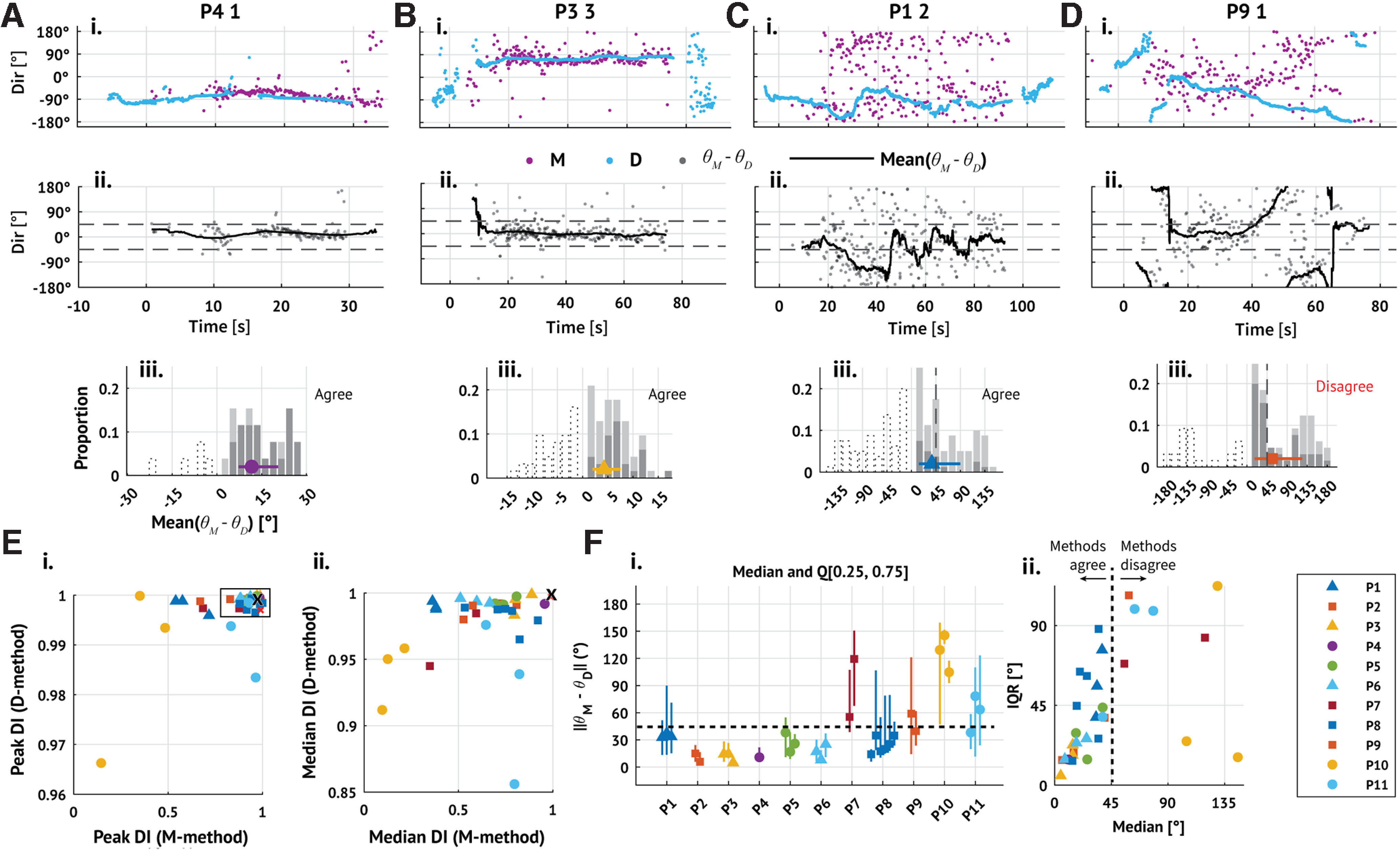
Existing methods produce consistent TW direction estimates for in vivo data. Ai–Di, Example TW directions inferred from 4 subjects and seizures estimated through time using both methods (pink represents max-descent method; blue represents group delay method; patient ID and seizure number indicated in plot title). Seizure onset occurs at time 0 s. Aii–Dii, Differences between the directions estimated by the max-descent method and the group-delays method (gray dots); traces represent the mean difference over 5 s sliding windows. Aiii–Diii, Summary histograms of the absolute mean differences between the max-descent and group-delay methods; bar height indicates the proportion of means in each bin, and bars are segmented into darker and lighter regions to indicate positive and negative means, respectively. Negative bins are also shown using dotted outlines. Marker and whisker represent the median and IQR of the absolute differences. A–C, Example seizures with consistent TW direction estimates between methods (median difference between methods is <45°). D, Example seizure with inconsistent direction estimates between methods. E, The 90th (Ei) and 50th (Eii) percentiles of the DI for each seizure estimated using each method (max-descent method, horizontal axis; group delay method, vertical axis). The black 'x' indicates the DI of the fixed source simulations. F, Median and IQR of the differences between estimated directions in each seizure. Fi, Markers indicate the median difference between estimates; vertical lines indicate first and third quartiles. Fii, Same as in Fi, but with medians plotted along the horizontal axis and IQR along the vertical axis. E, F, Marker color and shape represent patient identity (see legend). Triangular markers represent surgeries performed in Boston (Massachusetts General Hospital or Brigham Women's Hospital). Circular and square markers represent surgeries performed at Columbia University Irving Medical Center.

Figure 3.

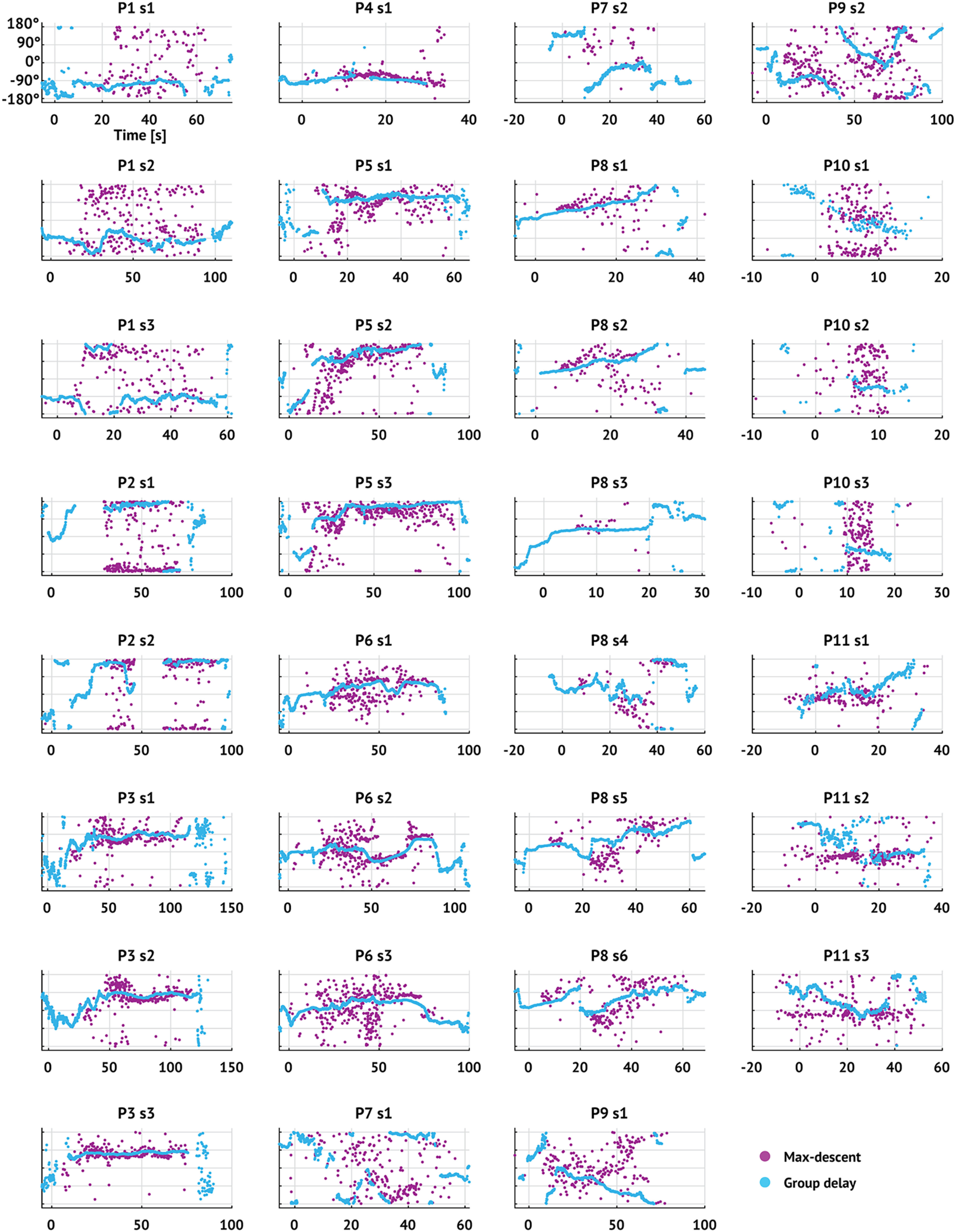
TW direction estimates through time using both methods for all seizures. Dots represent TW direction estimates (pink represents max-descent method; blue represents group delay method) versus time. Figure titles indicate patient label and seizure number. Seizure onset occurs at time 0 s.

To understand first whether results from the in vivo and synthetic data agree, we compare the DI estimated from the in vivo data to that estimated from the fixed source simulations. Specifically, we estimate the DI on 5 s sliding intervals (4 s overlap) during each seizure and compare the most stable intervals (DI values exceeding the 90th percentile; P₉₀(DI)) to the mean DI from the fixed source simulations (Fig. 2Ei). Across all seizures, the median value of P₉₀(DI) is near 1, consistent with the DI from the fixed source simulations for both methods (max-descent method median 0.92, IQR [0.744, 0.960]; group delay method median 0.999, IQR [0.997, 0.999]). Repeating this analysis using in vivo DI values exceeding the 50th percentile, we find that the group delay method continues to infer stable TW directions, while the max-descent method instead infers directions with substantially more variability (max-descent method median 0.69, IQR [0.51, 0.80]; group delay method median 0.99, IQR [0.98, 0.99]; Fig. 2Eii).

Next, we examine in the in vivo data the angular difference between the max-descent and group delay method direction estimates. For each seizure, we generate a set of per-discharge differences, the difference between the direction estimated by the max-descent method at each discharge and the nearest (in time) group delay method direction estimate, and compute the mean difference between the estimates on sliding 5 s intervals (4 s overlap). In a majority of seizures (23 of 31), the median value of the empirical distribution of differences during the seizure is <45° (median 32.8°, IQR [15.5, 51.4]°; Fig. 2Fi). To understand whether direction estimates from the two methods differ in a consistent way across time, we also examine for each seizure a dispersion in the differences (measured as the width of the IQR). Large dispersion suggests that the methods produce similar estimates during some intervals of the seizure, and comparably many dissimilar estimates during other intervals; small dispersion indicates a consistent difference between the methods throughout the seizure. Visual inspection shows that the dispersion tends to increase with the median difference between methods (Fig. 2Fii). When the median difference between methods is small, consistent estimates occur throughout the seizure (examples in Fig. 2A,B). As the dispersion increases, so does the median difference (example in Fig. 2C). When the median difference between methods is large, intervals of agreement and disagreement occur in comparable proportions throughout the seizure (example in Fig. 2D). We note that, in rare cases, the median difference is high relative to the dispersion (2 seizures from patient P10; Fig. 2Fii, yellow circles), suggesting a persistent difference between the estimates from each method.

We conclude that, while both methods detect intervals with highly stable (DI > 0.9) TW directions, estimates from the group delay method are more stable than the max-descent method, consistent with the simulation results. In most seizures, the mean difference between the methods fluctuates but tends to be <45°. These findings are consistent with the expected behavior of the methods when TW directions undergo periods of stability interspersed with rapid changes. During periods of stable TW direction, the methods agree, with high DI. During rapid changes in TW direction, the methods disagree as a rapid change in TW direction appears instantaneously in the max-descent method and more slowly in the group delay method.

IWs occur in most seizures

The results above show that TWs appear during seizures, consistent with previous studies (González-Ramírez et al., 2015; Wagner et al., 2015; Smith et al., 2016; Martinet et al., 2017; Liou et al., 2020; Diamond et al., 2021). However, the source producing these TWs remains controversial (Smith et al., 2016; Martinet et al., 2017; Proix et al., 2018; Schevon et al., 2019). One hypothesis posits that TWs emerge from an IW, a slowly propagating region characterized by tonic high MUA (i.e., high firing rates) and collapsing feedforward inhibition, that delineates the boundary between penumbral (inhibition intact) and recruited (inhibition collapsed) territories (Schevon et al., 2019). However, high tonic firing does not always demarcate the IW (Wagner et al., 2015; Schevon et al., 2019; Merricks et al., 2021) and to identify the IW recent studies have developed additional criteria associated with recruitment (Schevon et al., 2012, 2019; Weiss et al., 2013; Merricks et al., 2021). Because the full collection of optimal features that characterize the IW remains unknown, we here define the IW based solely on the presence of increased tonic firing (i.e., without additional inclusion criteria; see Materials and Methods). We then characterize the identified IWs and compare these results with existing descriptions.

We identify an IW in 20 of 31 seizures and 8 of 11 patients (examples in Fig. 4A; none detected in 3 patients: P2, P10, P11). We note that this set includes those seizures cited as evidence supporting the original IW hypothesis (subjects P4 and P5) (Schevon et al., 2012; Weiss et al., 2013; Smith et al., 2016). To compare the identified IWs with previous descriptions, we compute the peak firing rate (average peak firing rate across electrodes where the IW is detected), duration of the event (average event duration across electrodes where the IW is detected), and propagation speed (magnitude of velocity associated with plane of best fit; see Materials and Methods). We find that all three characteristics (Table 3) are consistent with previously reported results (reported firing rates ≈ 100 Hz; reported speeds ≈ 1 mm/s; reported durations ≈ 2 s; Fig. 4B) (Schevon et al., 2012; Smith et al., 2016) We conclude that an IW is a common feature near seizure onset in these data, in support of existing studies that examined a smaller number of cases (Schevon et al., 2012; Smith et al., 2016).

Figure 4.

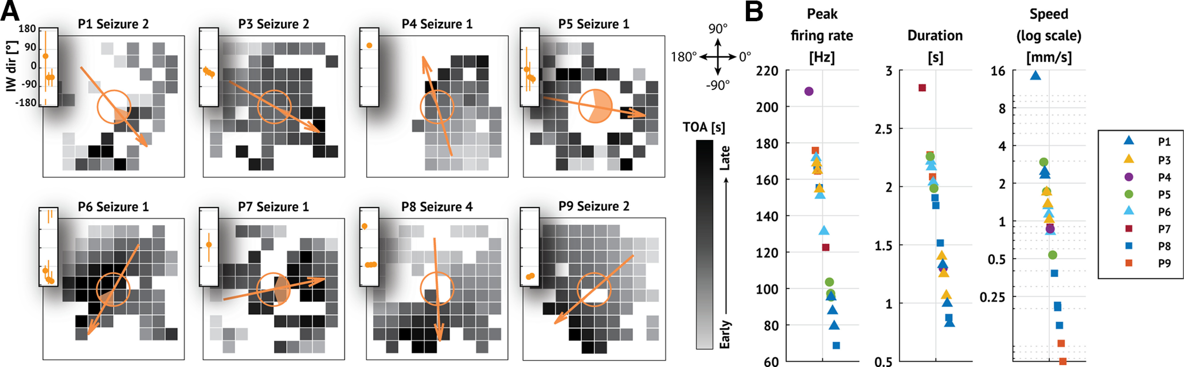
IWs are detected in a majority of seizures. A, Example recruitment patterns from each patient with an IW. In each subfigure, squares represent electrodes organized on a 10 × 10 MEA. Darker colors represent later recruitment times (i.e., time of arrival TOA; see scale bars), and missing squares represent electrodes where the IW was not detected. Arrows indicate direction of IW propagation. Shaded region of the open circles in the center of each subfigure represents 95% CIs of the estimated propagation direction (see Materials and Methods). Insets, IW direction with 95% CIs for each seizure of the patient shown. B, Peak firing rate, duration, and propagation speed of the IW detected in each seizure. Marker shape and color represent patient identity (see legend).

The IW has a transient impact on TW directions consistent with the IW hypothesis

Under the IW hypothesis, TW directions approximately align with the IW direction ahead of IW crossing, and then TW directions reverse after IW crossing (Smith et al., 2016; Schevon et al., 2019; Liou et al., 2020). To characterize how the IW affects fast TW directions, we consider the subset of patients and seizures with an IW (20 seizures with an IW, 8 patients) and examine the distributions of TW directions before and after IW crossing (examples in Fig. 5A). Visual inspection suggests a shift in TW directions near the IW crossing in some (e.g., P3 in Fig. 5A), but not all, seizures (e.g., P4 in Fig. 2A). In addition, before IW crossing, TW directions appear to align with the IW direction in some cases (examples in Fig. 5A), again consistent with the IW hypothesis.

Figure 5.

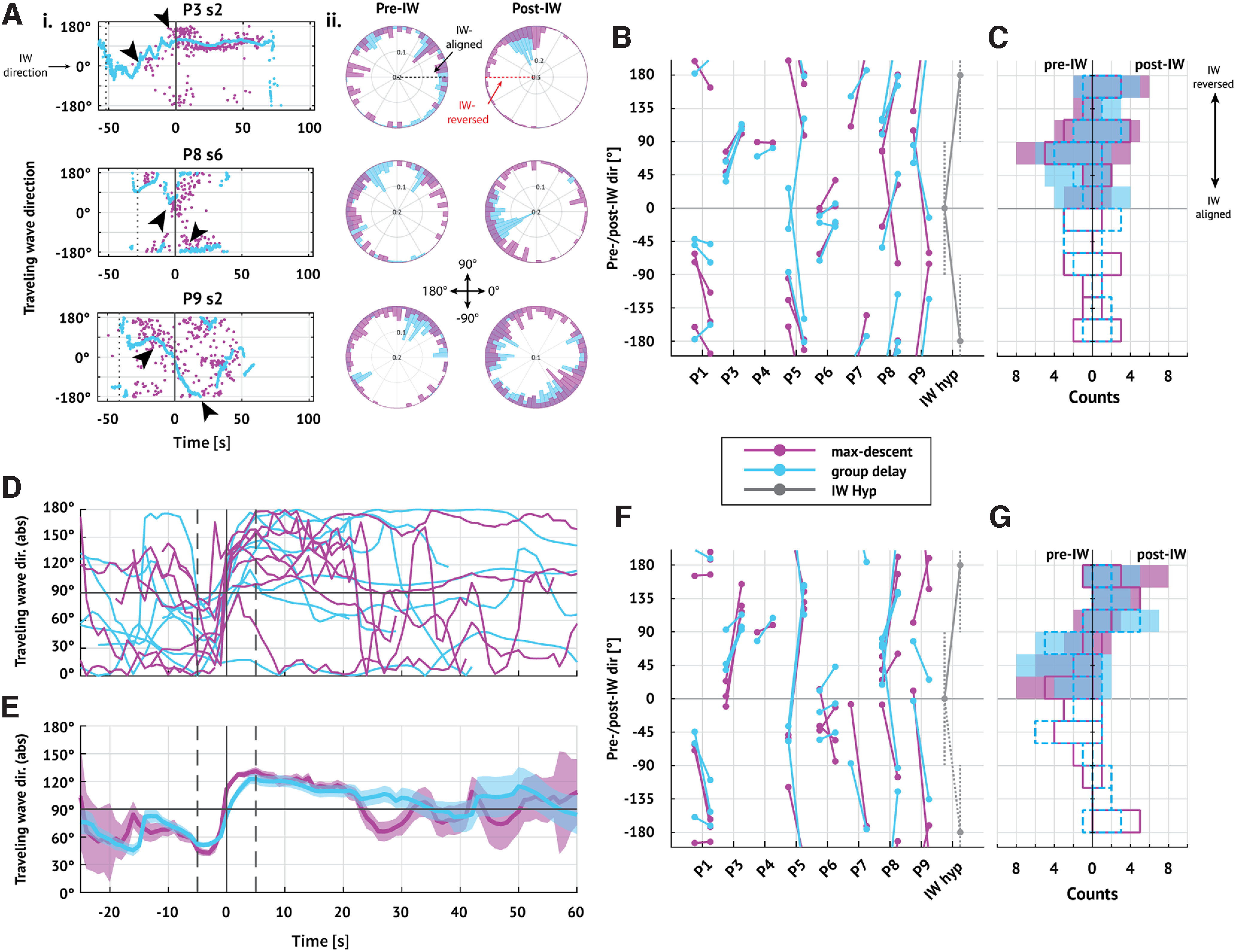
Fast TWs temporarily coordinate with the IW. A, TW directions through time oriented to the IW. Ai, Examples of TW directions through time in three seizures. Dots represent TW estimates (pink represents max-descent method; blue represents group delay method) with times and directions adjusted so that the IW occurs at 0 s (vertical line) with direction 0°. Visual inspection suggests that TW directions shift near IW crossing (arrows). Aii, Polar histograms of the distribution of TW directions before (left) and after (right) IW passage. In two examples, the post-IW distributions appear unimodal in the group delay method (first and second rows, blue bars); the other histograms represent complex or multimodal distributions. B, Changes in mean TW direction during pre- and post-IW epochs in each seizure. Each barbell represents the pre- and post-IW mean TW direction (pre-IW on the left; pink represents max-descent method; blue represents group delay method). Gray barbells represent the directions expected under the IW hypothesis. C, Summary of pre- and post-IW directions in all seizures. Histograms of mean (left) pre- and (right) post-IW directions. Outlined bars represent distribution of signed mean directions (solid pink line indicates max-descent method; dashed blue line indicates group delay method); shaded bars represent distribution of absolute value of mean directions (pink represents max-descent method; blue represents group delay method). A–C, All directions are rotated so that the IW direction is at 0°. D, Mean difference between TW direction and the IW direction through time in each patient using each method (pink represents max-descent method; blue represents group delay method). Time is aligned so that the IW occurs at t = 0 s; traces indicate the mean on sliding 5 s intervals (4.9 s overlap) for a given patient. E, Mean difference between TW and IW directions through time. Traces indicate jackknife estimates of the mean using estimated means from each patient; shaded regions represent 95% CI of the mean. Vertical bar at 0 s represents IW crossing time. TWs are more closely aligned with the IW just ahead of IW crossing (mean < 90° both methods, p < 0.05, jackknife estimator), then shift to more closely reversed just after IW passage (mean > 90° both methods, p < 0.05, jackknife estimator). D, E, Vertical solid line at 0 s indicates IW crossing time; vertical dashed lines indicate 5 s before and after IW crossing time. F, G, Same as in B, C, but for TW directions in limited 5 s intervals before (t in [−7.5, −2.5] s) and after (t in [2.5, 7.5] s) time of detected shift.

To test the IW hypothesis, we first divide each seizure into a pre-wavefront interval (from seizure onset until IW crossing) and a post-wavefront interval (from IW crossing until seizure termination). We then estimate the mean TW direction within each interval (N = 20 seizures with an IW, 8 patients). If the IW hypothesis holds, then we expect to find pre-wavefront mean directions within 90° of the IW direction (found in 12 of 20 and 15 of 20 seizures using the max-descent and group delay methods, respectively) and post-wavefront directions within 90° of the reversed IW direction (found in 12 of 20 seizures, both methods). We find that both pre-wavefront and post-wavefront alignment criteria hold in only 6 of 20 and 7 of 20 seizures using the max-descent and group delay methods, respectively (Fig. 5B,C). We conclude from these initial results that only limited evidence exists to support a sustained shift in TW direction at IW crossing.

Two factors may limit our ability to detect a shift in TW direction at IW crossing: (1) uncertainty in determining the IW crossing time and (2) transience of the IW effect on TW direction. To address these factors, we first identify for each seizure the time near (±10 s) IW crossing with the largest shift in alignment between TWs and the IW (see Materials and Methods). Second, we analyze the evolution of TW direction in sliding 5 s intervals (4.9 s overlap) from seizure onset to termination using a jackknife procedure (see Materials and Methods). Briefly, for a given interval, we compute the mean difference between the TW directions and the IW direction for each patient (θ_p; Fig. 5D). We then perform a leave-one-out procedure (leaving out each patient) to estimate the population mean (θ) with 95% CIs at each time point (Fig. 5E).

With these modifications, we find for both methods an interval of preferentially aligned TWs ahead of the IW (θ < 90°, p < 0.05, jackknife procedure; t in [−10, 0] s), followed by an interval of preferentially reversed TWs after IW crossing (θ > 90°, p < 0.05, jackknife procedure; t in [0, 20] s; Fig. 5E). Examining TW directions in limited epochs near the IW crossing time (pre: t in [−7.5, −2.5] s; post: t in [2.5, 7.5] s), we find shifts in TW direction that satisfy the pre-wavefront and post-wavefront alignment criteria in 12 of 20 (14 of 20) seizures (max-descent and group-delay methods, respectively; compared with 6 of 20 and 7 of 20 seizures when considering the full epochs; Fig. 5F,G). We conclude that, near IW crossing, there exists in a majority of seizures a shift in TW direction consistent with the IW hypothesis.

Beyond the interval of time directly surrounding IW crossing, both methods indicate fluctuations ∼90° of the mean TW direction. The transient relationship between the IW and TW directions may result from reduced accuracy of direction estimation. Both the group delay method and the max-descent method apply linear regression to estimate the direction of wave propagation. This regression approach may become inappropriate as the IW moves further from the MEA, reducing the number of time points with significant direction estimates (see Materials and Methods). To test for changes in regression accuracy over time, we examine the proportion of TWs detected (Fig. 6A) and RMSE of the linear model fits (Fig. 6B). Reduced alignment between fast TWs and the IW late in seizure may also result from increasing directional variability as the TW moves further from the IW. To test this, we also examine the DI through time (DI, Fig. 6C). Computing the slope of each statistic after IW crossing (t in [10, 50] s; see Fig. 6, right panels), we find no evidence of a consistent change (p = 0.19, two-tailed t test; Table 4). We conclude that insufficient evidence exists to support the hypothesis that reductions in signal-to-noise drive the transient relationship between the fast TW directions and IW directions. We note that performing the same analysis yields similar results for t in [10, 40] s or t > 10 s.

Figure 6.

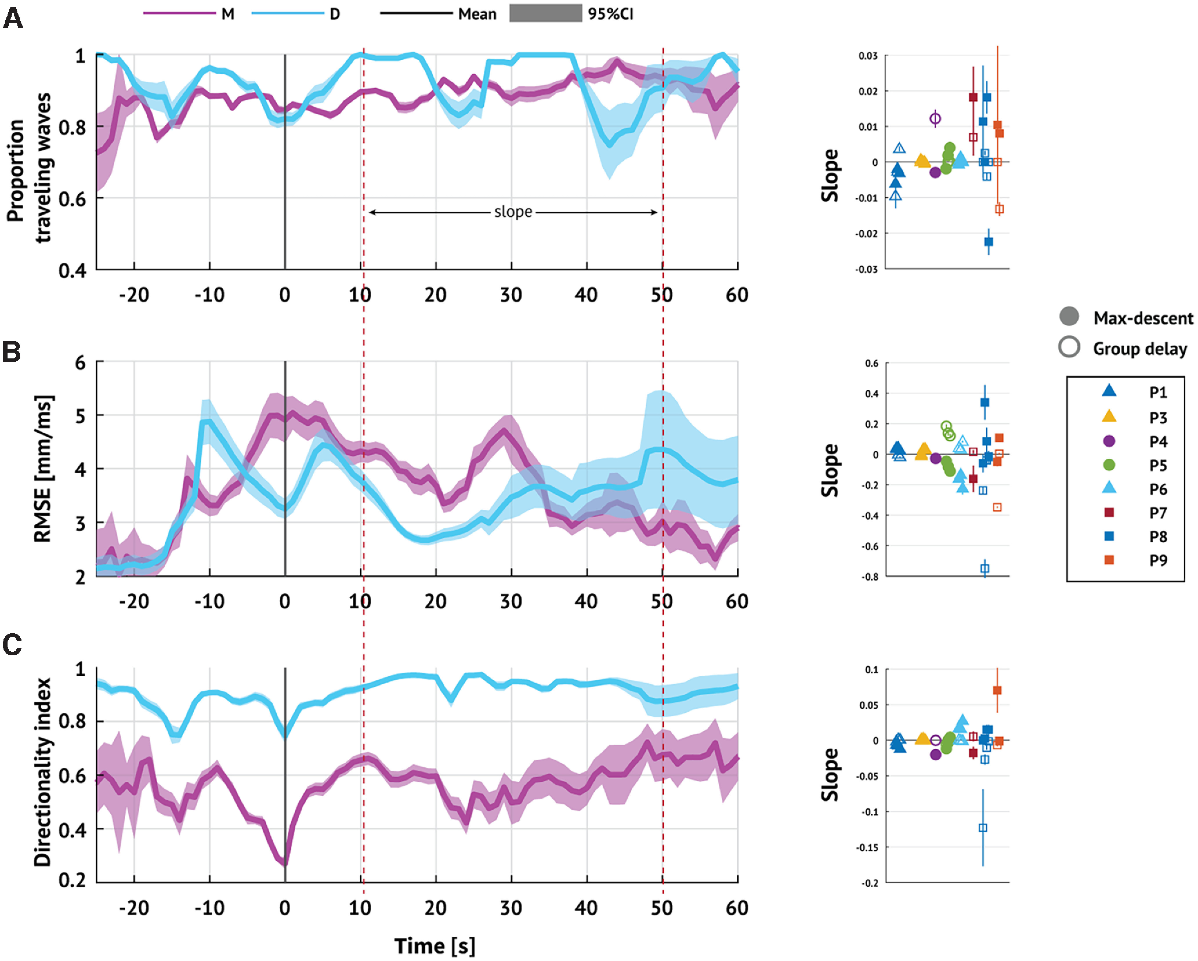
Reductions in signal-to-noise do not explain the transient relationship between TW and IW directions. Left, Expected proportion of (A) discharges classified as TWs, (B) RMSE of linear model fits, and (C) DI through time. Solid lines indicate estimated mean value. Shaded region represents 95% CI (pink represents max-descent method; blue represents group delay method). Right, For each metric and for each seizure, the slope of best linear regression fit for [10, 50] s. Marker shape and color represent patient ID. Filled (hollow) markers represent max-descent method (group delay method). IW crossing occurs at t = 0 s.

Table 4.

Summary of changes in signal characteristics^a

Validation metric	TOA method	Mean slope [95% CI]	pb
Proportion TW (unitless)	max-descent	0.0017 [−0.0024, 0.0059]	0.39
	group delay	−0.0003 [−0.0027, 0.0021]	0.8
RMSE (ms)	max-descent	−0.02 [−0.076, 0.037]	0.48
	group delay	−0.036 [−0.13, 0.06]	0.44
DI (unitless)	max-descent	0.0046 [−0.0046, 0.014]	0.31
	group delay	−0.0085 [−0.021, 0.0045]	0.19

^aEstimates of the mean and 95% CIs for the collection of slope estimates shown in Figure 6.

^bSignificance levels (i.e., p values) are computed using a one-sample two-tailed t test.

We conclude that, near IW crossing, a transient relationship exists between the TW and IW directions, consistent with the IW hypothesis: just before IW passage, the TW and IW directions align; and just after IW passage, the directions reverse.

Multiple shifts in TW direction occur during seizures

We have shown that a shift in TW directions coincides with IW crossing. However, this relationship is transient; as the seizure progresses beyond IW crossing, relationships between TW and IW directions become unclear. Visual inspection suggests that, in some seizures, multiple shifts in TW directions occur (examples in Fig. 5A). We now consider the properties of these stable TW directions and their relationships to the IW. We expect no more than one discrete shift in TW directions coinciding with the IW crossing over the MEA. More than one shift in TW directions suggests more complicated dynamics resulting from, for example, a partially dissipated IW or multiple interacting TW sources.

To assess these relationships, we first identify intervals where the TW directions are stable. To do so, we measure the DI on overlapping 5 s intervals (4.9 s overlap) throughout each seizure and consider an interval stable if the DI exceeds 0.5 (0.97) and lacks abrupt shifts in TW direction (max-descent method and group delay method, respectively; see Materials and Methods). We illustrate the stable intervals detected in an example seizure in Figure 7A. In this example, we detect 5 stable intervals, comprising 52% of the seizure (I*) such that the longest interval (the fourth interval) makes up 34% of the stable time (I^†_max). Stable intervals for all seizures are shown in Figures 8 and 9.

Figure 7.

Multiple shifts in TW direction occur during seizures. A, Example stable intervals from one seizure. Estimates of TW directions (small black circles represent max-descent method) organize into five stable intervals (sequences of large pink circles). Seizure duration (T) is the time from first to last detected TW. The interval from first TW detection to IW crossing is the pre-IW epoch (T_pre); the interval from IW crossing to the last TW detection is the post-IW epoch (T_post). The duration of each stable interval n is denoted I_n with the longest, or primary, interval denoted I_max. Bottom, Gray box represents example intervals. B, Number of stable intervals per seizure. Histograms oriented with counts on the horizontal axis. Pink (blue) histograms oriented to the left (right) represent results of analysis using the max-descent method (group delay method). Circles represent the median number of stable intervals detected across all seizures. C, Stability of TW direction during seizures. Histograms organized as in B. Circles represent median values. Ci–Ciii, Proportion of time with stable TW directions during the (Ci) entire seizure, (Cii) pre-IW epoch, and (Ciii) post-IW epoch. Civ, Average interval duration relative to seizure duration. Cv, Duration of primary interval relative to total time stable.

Across all patients and seizures with an IW (N = 20), the median number of intervals detected is 3 (Fig. 7B) and the median percentage of time stable is 52% (69%; max-descent and group delay methods, respectively; Fig. 7Ci). Before IW crossing, the median percentage of time with stable TW directions is 31% (55%) compared with 62% (69%) after IW crossing (max-descent and group delay methods, respectively; Fig. 7Cii,Ciii). We find that most stable intervals are transient; the average duration of an interval relative to seizure duration is 16% (24%; max-descent and group delay methods, respectively; Fig. 7Civ). We also find that a single stable interval dominates the total time stable; the longest stable interval makes up 66% of the total time stable (77%; max-descent and group delay methods, respectively; Fig. 7Cv). We note that the longest stable interval is the last stable interval in 15 of 20 (9 of 20) seizures (max-descent method and group delay method, respectively).

To summarize, we find in a majority of seizures (12 of 20 max-descent method, 13 of 20 group delay method; Fig. 7B) at least three stable intervals, consistent with dynamics resulting from multiple focal TW source locations. TW directions tend to remain stable throughout large portions of a seizure, more so after IW crossing, and the amount of time stable tends to be dominated by a single stable interval. We conclude that one main TW source typically dominates the dynamics, accompanied by one or more transient sources.

A framework to unify the two competing theories of TW origin

While our analysis reveals features of TW activity consistent with the IW hypothesis, we also show that TWs arise from multiple source locations. In particular, we observe in many seizures a dominant source direction combined with one or more transient source directions. Because this dominant source direction can last as long as 50 s (example in Fig. 10A), we propose an updated hypothesis in which a fixed source and IW interact. To illustrate this proposal, we consider an example (P3 s2, max-descent method) in which the seizure progresses through three intervals of stable TWs, each with a distinct direction (Fig. 10A). In this example, TWs first propagate outward ahead of the IW, and the TW direction is IW-aligned (Φ_A, illustration in Fig. 10Ai). Then, as the IW crosses the MEA, the TW direction changes to propagate in the IW-reversed direction (Φ_R; Fig. 10Aii). Finally, as the influence of the IW fades, TWs propagate from a fixed source (Φ_F; Fig. 10Aiii).

Figure 10.

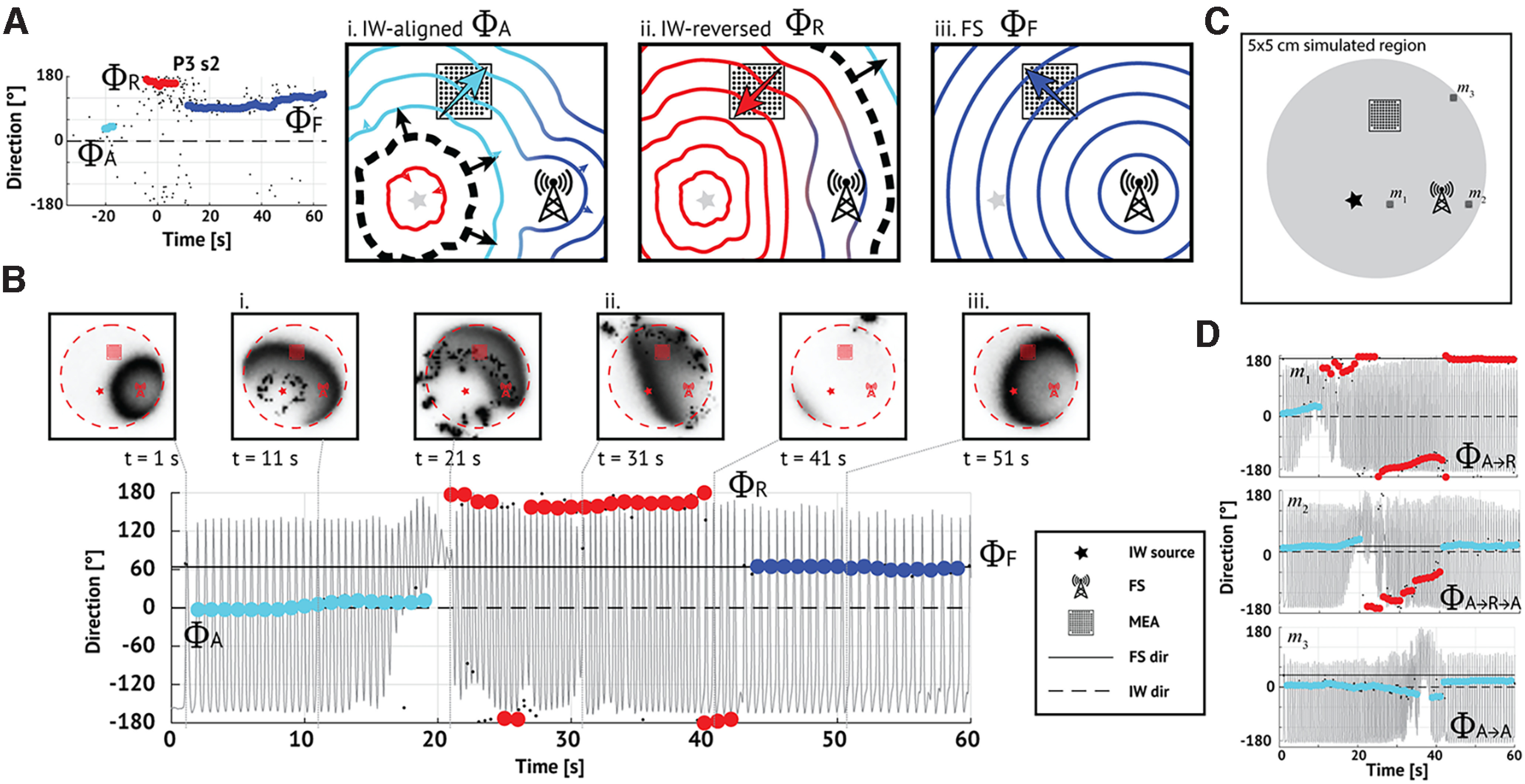
A model combining a fixed and IW source produces complex progressions of TW directions. A, Example in vivo seizure containing two shifts and three stable intervals, each with distinct directions (labeled Φ_A,R,F and indicated as light blue, red, and dark blue dots, respectively). This progression may reflect the combined influences of a fixed source (FS, Ai–Aiii, radio tower pictogram) and an expanding IW (Ai–Aiii, black dashed line, arrows indicating IW propagation). The square grid represents the MEA. In this schematic, (Ai) TWs (light blue contours) initially align with the IW (direction Φ_A, light blue arrow). Aii, After the IW crosses the MEA, TWs (red contours) reverse direction (direction Φ_R, red arrow). Aiii, Once the IW dissipates, only TWs (dark blue contours) from the fixed source remain (direction Φ_F, dark blue arrow). B, A simulation reproducing the Φ_A→Φ_R→Φ_F progression observed in vivo. During a simulated seizure, TW directions (max-descent method, direction 0° indicating the IW direction) shift from (Bi) IW-aligned (Φ_A, light blue dots), to (Bii) IW-reversed (Φ_R, red dots), to (Biii) FS-aligned (Φ_F, dark blue dots). Horizontal dashed and solid lines indicate relative directions of IW source (0°, Φ_A) and fixed source (45°, Φ_F), respectively. Gray trace represents the simulated firing rate of the excitatory cell population. Panels above represent images of the excitatory cell population activity on the cortical surface at 10 s intervals; dark (light) shades represent high (low) activity; the red dashed circle encompasses the irritative zone; and the star, square, and radio tower represent the IW source, MEA, and fixed source, respectively (see legend). C, Geometry of the simulation shown in B. The IW source (star), fixed source (radio tower), and MEA (grid) organized in a triangular configuration. An irritative zone (gray circle) lies within the cortical surface (black square). The locations indicated with black squares (labeled m₁, m₂, m₃) correspond to alternative MEA placements shown in D. D, Alternative placement of the MEA leads to different TW direction progressions. When Φ_F = Φ_R (location m₁ in C), the TW directions progress Φ_A→Φ_R. When Φ_F = Φ_A (location m₂ in C), the TWs progress Φ_A→Φ_R→Φ_A. The MEA at the boundary of the irritative zone (location m₃ in C), coupled with the geometry here, results in TW directions that appear fixed.

To simulate this proposed scenario, we consider the neural mass model in Martinet et al. (2017). We model the irritative zone as a subregion with persistent increased drive to the excitatory cell population (4.1 cm diameter; 1.2 mV increase in the resting membrane potential of the excitatory population). Within the irritative zone, we model the fixed source as a focal region with increased excitatory drive during the seizure (5 mm diameter; 1.7 mV increase in the resting membrane potential of the excitatory population). We model the IW as a slowly expanding (1 mm/s) front of suppressed inhibition (the firing rates of the inhibitory populations decrease from 60 to 40 Hz), which results in increased excitatory population activity (Trevelyan et al., 2006; Schevon et al., 2012; Liou et al., 2020) (see Materials and Methods). We simulate a 60 s seizure (Fig. 10B) with the IW source (the location where the IW first appears), fixed source, and MEA located in a triangular configuration with each ∼2 cm apart (Fig. 10C). At seizure onset, we first briefly detect TWs propagating from the fixed source (Fig. 10B, t = 2 s). Then, the IW expands and becomes the dominant source of TWs (t in [2, 20] s); TWs propagate away from the IW in both directions (inward and outward) so that TW directions are initially IW-aligned (Φ_Α, Fig. 10Bi). After IW crossing (t = 25 s), the TW directions reverse (Φ_R, Fig. 10Bii). When the IW expands beyond the irritative zone, the TW directions change again, reflecting the influence of the fixed source (t > 40 s, Fig. 10Biii). We note the qualitative agreement between this simulated seizure (Fig. 10B) and the in vivo example (Fig. 10A); both display three stable intervals of TW direction (corresponding to the sequence {Φ_A, Φ_R, Φ_F}), with changes consistent with both an IW and fixed source.

Different placements of the MEA, with unmodified IW source and fixed source locations, produce different time evolutions of TW directions. For example, when arranged collinearly, the two sources are difficult to distinguish. Locating the MEA between the IW source and the fixed source (Fig. 10C, location m₁), Φ_F equals Φ_R, so that TW directions appear with the progression Φ_AΦ_R (Fig. 10D, m₁). Locating the MEA collinear with, but beyond the fixed source and IW source (Fig. 10C, location m₂), Φ_F equals Φ_A, so TW directions appear with the progression Φ_AΦ_RΦ_A (Fig. 10D, m₂). Locating the MEA on the boundary of the irritative zone (Fig. 10C, location m₃), few TWs propagate in the Φ_R direction, and the Φ_A and Φ_F directions dominate. However, given the geometry in this simulation with Φ_A and Φ_F <45° apart and the MEA located far from the sources, these directions are difficult to distinguish, resulting in TWs appearing to propagate from a fixed source (Fig. 10D, m₃). These examples illustrate that interactions between an IW and a fixed source can produce complex progressions of TW directions, consistent with those observed in the data. In addition, the placement of the MEA can dramatically change the observed progressions, to produce TW dynamics consistent with each, or neither, existing theory.

Discussion

While TWs appear common during seizures (González-Ramírez et al., 2015; Wagner et al., 2015; Smith et al., 2016; Martinet et al., 2017; Liou et al., 2020; Diamond et al., 2021), whether these waves arise from a fixed source (Martinet et al., 2017) or slowly expanding wavefront (Smith et al., 2016) remains unclear. Because of the limited MEA recordings studied by each group (N = 3 subjects in Smith et al., 2016; N = 3 subjects in Martinet et al., 2017), and the different analysis methods developed and applied, whether the conflicting conclusions reflect patient- or method-specific characteristics remained unclear. To resolve this dispute, we investigated the relationship between the IW and the direction of fast TWs during human seizures using the combined data and methods from both groups (Smith et al., 2016; Martinet et al., 2017). Doing so, we reproduced many results from the existing literature, including evidence that TWs coordinate with an IW (Trevelyan et al., 2007; Smith et al., 2016; Liou et al., 2020), and evidence of long-lasting TW sources (Martinet et al., 2017). However, we also found evidence that both existing theories failed to capture the complete range of spatiotemporal dynamics observed. We showed that the relationship between the IW and TWs was transient and persisted only near the time of IW crossing, and that seizures exhibit multiple stable directions of TWs, consistent with an interplay between TW sources at multiple locations. To address these limitations, we combined the two existing theories in a new model consisting of both an IW and fixed source of TWs, and showed in simulation how this model produced multiple patterns of TW dynamics consistent with the scenarios observed in vivo.

The IW has been proposed as the mechanism driving cortical seizure spread and termination (Eissa et al., 2017; Parrish et al., 2019; Schevon et al., 2019; Liou et al., 2020). At the boundary between functional and collapsed inhibition, the IW generates the aberrant TW dynamics associated with propagating ictal discharges observed during seizures. Here, we present more evidence that a relationship between the IW and TW extends beyond slice recordings (Trevelyan et al., 2006, 2007; Chiang et al., 2018; Wenzel et al., 2019) or a specific small set of patients (Schevon et al., 2012; Weiss et al., 2013; Smith et al., 2016; Liou et al., 2020; Merricks et al., 2021). However, directly testing the hypothesis that the IW generates ictal TWs remains a challenge. We note that patients with slow or undetected IWs tend to produce TW direction estimates with greater variability and less agreement between estimation methods (e.g., see P7, P10, and P11 in Fig. 2). Clinically, these patients also differ: P7, P10, and P11 all have MEAs located in the frontal lobe (Table 1). While intriguing, the small number of patients available here limits confidence in these preliminary observations.

To model the TWs that propagate during seizures, we simulated both an IW and a fixed source. Doing so, we mimicked many features observed in vivo, including the following: the passage of an IW with transient TW alignment, the emergence of multiple stable TW directions, and the existence of a dominant TW direction. However, we note that no unique solution exists for the observed TW dynamics. For example, the emergence of a stable TW source after IW passage could result from the following: the appearance of a coexisting fixed source temporarily obscured by the IW (as we simulated) or uneven dissipation of the IW resulting in a spatially localized TW source. While the IW might obscure a coexisting fixed source, strong excitatory inputs from the IW could instead initiate a secondary fixed source (Liou et al., 2018). Although limited spatial coverage of the MEA prevents investigation of these different scenarios, application of existing source localization techniques (Kim et al., 2010; Weiss et al., 2013; Becker et al., 2014; Diamond et al., 2021; Li et al., 2021) could provide additional insight by identifying the cortical locations of each wave source. An increase in MUA, which may manifest as high gamma activity (Mukamel et al., 2005; Rasch et al., 2008; Weiss et al., 2013), at each source would provide additional evidence to support each TW source.

Beyond the existing hypothesized role of the IW, we identified additional cortical features involved in the progression and maintenance of TWs during seizures. Specifically, we identified multiple stable TW directions during seizures and proposed that each stable direction corresponded to a cortical seizure source. This proposal is consistent with the concept of a seizure network, in which multiple sources of seizure activity (Liou et al., 2018; Diamond et al., 2021) evolve over the large-scale brain network (Davis et al., 2021), a concept that remains debated (Zaveri et al., 2020; Davis et al., 2021). To analyze this network, we consider MEA recordings, which reveal only a small portion of the brain network. However, because macroscopic TWs dominate these brain dynamics late in seizure, the propagation of these waves over the MEAs provides insights into their network source. We note that the limited spatial coverage of the MEA also prevents testing the assumption that similar dynamics occur across cortex. However, the consistency of results across patients, with different MEA locations, and the consistency of TW dynamics across MEA and macroelectrode recordings (Martinet et al., 2017) support the generalizability of these results.

To simulate these multisource seizures, we developed a biophysically-motivated computational model that incorporates the two proposed sources of TWs: a slowly moving IW (Schevon et al., 2012; Smith et al., 2016; Liou et al., 2020) and a fixed source (Martinet et al., 2017). The model reproduces the diversity of trends observed in the progression of TW directions via manipulation of the relative locations of an IW, fixed source, and recording array. This proposal differs from a recently developed phenomenological model (the Epileptor field model) in which changes in the location of the TW source result from reorganization of the phases of the neural oscillators (Proix et al., 2018). The two modeling approaches provide complementary mathematical and biophysical perspectives; future work may further unify these perspectives.

Surgical treatment for epilepsy remains imperfect; following resective surgery seizures return in 70% of patients without a brain lesion, and up to 40% of patients with a clear structural lesion (Rosenow and Lüders, 2001; Cohen-Gadol et al., 2006; Jeha et al., 2007; Wetjen et al., 2009). We propose that, if the sources of TWs serve as fundamental nodes in the seizure network, then some of the TW sources may provide therapeutic targets in the seizure network. If a single source generates TWs, then targeting this source (i.e., resecting a fixed source or the initial IW source) might reduce seizure recurrence. Targeting the source of ictal TWs (Diamond et al., 2021), the source of propagating interictal ripples (80-250 Hz events) (Tamilia et al., 2021), or the source of propagating interictal discharges (Alarcon, 1997; Mitsuhashi et al., 2021) has been shown to improve surgical outcomes. Alternatively, if multiple TW sources exist, then we hypothesize that treating each source (e.g., as multiple responsive neurostimulation [RNS] targets) (Sisterson et al., 2019), or a sufficient subset of sources, may disrupt the seizure network and prevent the pathologic TW dynamics. Whether targeting IW sources or fixed sources improves the chances of successful treatment remains unknown; future work is required to compare treatment outcomes with the number and type of TW sources removed. Extending these observations to include dynamics on an anatomic or functional connectome may provide additional insights (Jirsa et al., 2017; Sinha et al., 2017; Proix et al., 2018; Hashemi et al., 2020; Mitsuhashi et al., 2021), including pathways for nonlocal TW and source propagation (Shah et al., 2019; Wenzel et al., 2019), personalized to a patient's brain network model (An et al., 2019). Continuing work to understand the sources of TWs during seizures, and to link these sources to epilepsy treatment, promises novel therapeutic strategies for patient care.

References

- Alarcon G (1997) Origin and propagation of interictal discharges in the acute electrocorticogram: implications for pathophysiology and surgical treatment of temporal lobe epilepsy. Brain 120:2259–2282. 10.1093/brain/120.12.2259 [DOI] [PubMed] [Google Scholar]
- An S, Bartolomei F, Guye M, Jirsa V (2019) Optimization of surgical intervention outside the epileptogenic zone in the Virtual Epileptic Patient (VEP). PLoS Comput Biol 15:e1007051. 10.1371/journal.pcbi.1007051 [DOI] [PMC free article] [PubMed] [Google Scholar]
- Becker H, Albera L, Comon P, Haardt M, Birot G, Wendling F, Gavaret M, Bénar CG, Merlet I (2014) EEG extended source localization: tensor-based vs. conventional methods. Neuroimage 96:143–157. 10.1016/j.neuroimage.2014.03.043 [DOI] [PubMed] [Google Scholar]
- Berens P (2009) CircStat: a MATLAB toolbox for circular statistics. J Stat Soft 31:1–21. 10.18637/jss.v031.i10 [DOI] [Google Scholar]
- Bokil H, Andrews P, Kulkarni JE, Mehta S, Mitra PP (2010) Chronux: a platform for analyzing neural signals. J Neurosci Methods 192:146–151. 10.1016/j.jneumeth.2010.06.020 [DOI] [PMC free article] [PubMed] [Google Scholar]
- Buzsáki G, Anastassiou CA, Koch C (2012) The origin of extracellular fields and currents: EEG, ECoG, LFP and spikes. Nat Rev Neurosci 13:407–420. 10.1038/nrn3241 [DOI] [PMC free article] [PubMed] [Google Scholar]
- Chiang CC, Wei X, Ananthakrishnan AK, Shivacharan RS, Gonzalez-Reyes LE, Zhang M, Durand DM (2018) Slow moving neural source in the epileptic hippocampus can mimic progression of human seizures. Sci Rep 8:1564. 10.1038/s41598-018-19925-7 [DOI] [PMC free article] [PubMed] [Google Scholar]
- Cohen-Gadol AA, Wilhelmi BG, Collignon F, White JB, Britton JW, Cambier DM, Christianson TJ, Marsh WR, Meyer FB, Cascino GD (2006) Long-term outcome of epilepsy surgery among 399 patients with nonlesional seizure foci including mesial temporal lobe sclerosis. J Neurosurg 104:513–524. 10.3171/jns.2006.104.4.513 [DOI] [PubMed] [Google Scholar]
- Davis KA, Jirsa VK, Schevon CA (2021) Wheels within wheels: theory and practice of epileptic networks. Epilepsy Curr 21:243–247. 10.1177/15357597211015663 [DOI] [PMC free article] [PubMed] [Google Scholar]
- Diamond JM, Diamond BE, Trotta MS, Dembny K, Inati SK, Zaghloul KA (2021) Travelling waves reveal a dynamic seizure source in human focal epilepsy. Brain 144:1751–1763. 10.1093/brain/awab089 [DOI] [PMC free article] [PubMed] [Google Scholar]
- Eissa TL, Dijkstra K, Brune C, Emerson RG, van Putten MJ, Goodman RR, McKhann GM, Schevon CA, van Drongelen W, van Gils SA (2017) Cross-scale effects of neural interactions during human neocortical seizure activity. Proc Natl Acad Sci USA 114:10761–10766. 10.1073/pnas.1702490114 [DOI] [PMC free article] [PubMed] [Google Scholar]
- Eissa TL, Schevon CA, Emerson RG, McKhann GM, Goodman RR, Van Drongelen W (2018) The relationship between ictal multi-unit activity and the electrocorticogram. Int J Neural Syst 28:1850027. 10.1142/S0129065718500272 [DOI] [PubMed] [Google Scholar]
- Engel AK, Moll CK, Fried I, Ojemann GA (2005) Invasive recordings from the human brain: clinical insights and beyond. Nat Rev Neurosci 6:35–47. 10.1038/nrn1585 [DOI] [PubMed] [Google Scholar]
- Frauscher B, Bartolomei F, Kobayashi K, Cimbalnik J, van't Klooster MA, Rampp S, Otsubo H, Höller Y, Wu JY, Asano E, Engel J, Kahane P, Jacobs J, Gotman J (2017) High-frequency oscillations: the state of clinical research. Epilepsia 58:1316–1329. 10.1111/epi.13829 [DOI] [PMC free article] [PubMed] [Google Scholar]
- González-Ramírez LR, Ahmed OJ, Cash SS, Wayne CE, Kramer MA (2015) A biologically constrained, mathematical model of cortical wave propagation preceding seizure termination. PLoS Comput Biol 11:e1004065. 10.1371/journal.pcbi.1004065 [DOI] [PMC free article] [PubMed] [Google Scholar]
- Gotman J (1983) Measurement of small time differences between EEG channels: method and application to epileptic seizure propagation. Electroencephalogr Clin Neurophysiol 56:501–514. 10.1016/0013-4694(83)90235-3 [DOI] [PubMed] [Google Scholar]
- Hashemi M, Vattikonda A, Sip V, Guye M, Bartolomei F, Woodman MM, Jirsa VK (2020) The Bayesian Virtual Epileptic Patient: a probabilistic framework designed to infer the spatial map of epileptogenicity in a personalized large-scale brain model of epilepsy spread. Neuroimage 217:116839. 10.1016/j.neuroimage.2020.116839 [DOI] [PubMed] [Google Scholar]
- Hoaglin DC, Mosteller F, Tukey JW (1983) Understanding robust and exploratory data analysis. New York: Wiley. [Google Scholar]
- Jeha LE, Najm I, Bingaman W, Dinner D, Widdess-Walsh P, Lüders H (2007) Surgical outcome and prognostic factors of frontal lobe epilepsy surgery. Brain 130:574–584. 10.1093/brain/awl364 [DOI] [PubMed] [Google Scholar]
- Jirsa VK, Proix T, Perdikis D, Woodman MM, Wang H, Gonzalez-Martinez J, Bernard C, Bénar C, Guye M, Chauvel P, Bartolomei F (2017) The virtual epileptic patient: individualized whole-brain models of epilepsy spread. Neuroimage 145:377–388. 10.1016/j.neuroimage.2016.04.049 [DOI] [PubMed] [Google Scholar]
- Kim JS, Im CH, Jung YJ, Kim EY, Lee SK, Chung CK (2010) Localization and propagation analysis of ictal source rhythm by electrocorticography. Neuroimage 52:1279–1288. 10.1016/j.neuroimage.2010.04.240 [DOI] [PubMed] [Google Scholar]
- Kleen JK, Chung JE, Sellers KK, Zhou J, Triplett M, Lee K, Tooker A, Haque R, Chang EF (2021) Bidirectional propagation of low frequency oscillations over the human hippocampal surface. Nat Commun 12:2764. 10.1038/s41467-021-22850-5 [DOI] [PMC free article] [PubMed] [Google Scholar]
- Kobayashi E, Hawco CS, Grova C, Dubeau F, Gotman J (2006) Widespread and intense BOLD changes during brief focal electrographic seizures. Neurology 66:1049–1055. 10.1212/01.wnl.0000204232.37720.a4 [DOI] [PubMed] [Google Scholar]
- Kramer MA, Truccolo W, Eden UT, Lepage KQ, Hochberg LR, Eskandar EN, Madsen JR, Lee JW, Maheshwari A, Halgren E, Chu CJ, Cash SS (2012) Human seizures self-terminate across spatial scales via a critical transition. Proc Natl Acad Sci USA 109:21116–21121. 10.1073/pnas.1210047110 [DOI] [PMC free article] [PubMed] [Google Scholar]
- Li A, Huynh C, Fitzgerald Z, Cajigas I, Brusko D, Jagid J, Claudio AO, Kanner AM, Hopp J, Chen S, Haagensen J, Johnson E, Anderson W, Crone N, Inati S, Zaghloul KA, Bulacio J, Gonzalez-Martinez J, Sarma SV (2021) Neural fragility as an EEG marker of the seizure onset zone. Nat Neurosci 24:1465–1474. 10.1038/s41593-021-00901-w [DOI] [PMC free article] [PubMed] [Google Scholar]
- Liou J, Ma H, Wenzel M, Zhao M, Baird-Daniel E, Smith EH, Daniel A, Emerson R, Yuste R, Schwartz TH, Schevon CA (2018) Role of inhibitory control in modulating focal seizure spread. Brain 141:2083–2097. 10.1093/brain/awy116 [DOI] [PMC free article] [PubMed] [Google Scholar]
- Liou JY, Smith EH, Bateman LM, McKhann GM, Goodman RR, Greger B, Davis TS, Kellis SS, House PA, Schevon CA (2017) Multivariate regression methods for estimating velocity of ictal discharges from human microelectrode recordings. J Neural Eng 14:044001. 10.1088/1741-2552/aa68a6 [DOI] [PMC free article] [PubMed] [Google Scholar]
- Liou J, Smith EH, Bateman LM, Bruce SL, McKhann GM, Goodman RR, Emerson RG, Schevon CA, Abbott L (2020) A model for focal seizure onset, propagation, evolution, and progression. Elife 9:e50927. 10.7554/Elife.50927 [DOI] [PMC free article] [PubMed] [Google Scholar]
- Lüders HO, Najm I, Nair D, Widdess-Walsh P, Bingman W (2006) The epileptogenic zone: general principles. Epileptic Disord 8:1–9. [PubMed] [Google Scholar]
- Maronna RA, Martin RD, Yohai VJ, Salibián-Barrera M (2019) Robust statistics: theory and methods (with R). Available at http://ebookcentral.proquest.com/lib/bu/detail.action?docID=5568377 [Accessed September 18, 2021].
- Martinet LE, Fiddyment G, Madsen JR, Eskandar EN, Truccolo W, Eden UT, Cash SS, Kramer MA (2017) Human seizures couple across spatial scales through travelling wave dynamics. Nat Commun 8:14896. 10.1038/ncomms14896 [DOI] [PMC free article] [PubMed] [Google Scholar]
- Merricks EM, Smith EH, McKhann GM, Goodman RR, Bateman LM, Emerson RG, Schevon CA, Trevelyan AJ (2015) Single unit action potentials in humans and the effect of seizure activity. Brain 138:2891–2906. 10.1093/brain/awv208 [DOI] [PMC free article] [PubMed] [Google Scholar]
- Merricks EM, Smith EH, Emerson RG, Bateman LM, McKhann GM, Goodman RR, Sheth SA, Greger B, House PA, Trevelyan AJ, Schevon CA (2021) Neuronal firing and waveform alterations through ictal recruitment in humans. J Neurosci 41:766–779. 10.1523/JNEUROSCI.0417-20.2020 [DOI] [PMC free article] [PubMed] [Google Scholar]
- Mitsuhashi T, Sonoda M, Sakakura K, Jeong J, Luat AF, Sood S, Asano E (2021) Dynamic tractography-based localization of spike sources and animation of spike propagations. Epilepsia 62:2372–2384. 10.1111/epi.17025 [DOI] [PMC free article] [PubMed] [Google Scholar]
- Mukamel R, Gelbard H, Arieli A, Hasson U, Fried I, Malach R (2005) Coupling between neuronal firing, field potentials, and FMRI in human auditory cortex. Science 309:951–954. 10.1126/science.1110913 [DOI] [PubMed] [Google Scholar]
- Parrish RR, Codadu NK, Mackenzie-Gray Scott C, Trevelyan AJ (2019) Feedforward inhibition ahead of ictal wavefronts is provided by both parvalbumin- and somatostatin-expressing interneurons. J Physiol 597:2297–2314. 10.1113/JP277749 [DOI] [PMC free article] [PubMed] [Google Scholar]
- Proix T, Jirsa VK, Bartolomei F, Guye M, Truccolo W (2018) Predicting the spatiotemporal diversity of seizure propagation and termination in human focal epilepsy. Nat Commun 9:1088. 10.1038/s41467-018-02973-y [DOI] [PMC free article] [PubMed] [Google Scholar]
- Rasch MJ, Gretton A, Murayama Y, Maass W, Logothetis NK (2008) Inferring spike trains from local field potentials. J Neurophysiol 99:1461–1476. 10.1152/jn.00919.2007 [DOI] [PubMed] [Google Scholar]
- Rosenow F, Lüders H (2001) Presurgical evaluation of epilepsy. Brain 124:1683–1700. 10.1093/brain/124.9.1683 [DOI] [PubMed] [Google Scholar]
- Schevon CA, Weiss SA, McKhann G, Goodman RR, Yuste R, Emerson RG, Trevelyan AJ (2012) Evidence of an inhibitory restraint of seizure activity in humans. Nat Commun 3:1060. 10.1038/ncomms2056 [DOI] [PMC free article] [PubMed] [Google Scholar]
- Schevon CA, Tobochnik S, Eissa T, Merricks E, Gill B, Parrish RR, Bateman LM, McKhann GM, Emerson RG, Trevelyan AJ (2019) Multiscale recordings reveal the dynamic spatial structure of human seizures. Neurobiol Dis 127:303–311. 10.1016/j.nbd.2019.03.015 [DOI] [PMC free article] [PubMed] [Google Scholar]
- Shah P, Ashourvan A, Mikhail F, Pines A, Kini L, Oechsel K, Das SR, Stein JM, Shinohara RT, Bassett DS, Litt B, Davis KA (2019) Characterizing the role of the structural connectome in seizure dynamics. Brain 142:1955–1972. 10.1093/brain/awz125 [DOI] [PMC free article] [PubMed] [Google Scholar]
- Sinha N, Dauwels J, Kaiser M, Cash SS, Westover MB, Wang Y, Taylor PN (2017) Predicting neurosurgical outcomes in focal epilepsy patients using computational modelling. Brain 140:319–332. 10.1093/brain/aww299 [DOI] [PMC free article] [PubMed] [Google Scholar]
- Sisterson ND, Wozny TA, Kokkinos V, Constantino A, Richardson RM (2019) Closed-loop brain stimulation for drug-resistant epilepsy: towards an evidence-based approach to personalized medicine. Neurotherapeutics 16:119–127. 10.1007/s13311-018-00682-4 [DOI] [PMC free article] [PubMed] [Google Scholar]
- Smith EH, Liou J, Merricks EM, Davis T, Thomson K, Greger B, House P, Emerson RG, Goodman R, McKhann GM, Sheth S, Schevon C, Rolston JD (2022) Human interictal epileptiform discharges are bidirectional traveling waves echoing ictal discharges. Elife 11:e73541. 10.7554/Elife.73541 [DOI] [PMC free article] [PubMed] [Google Scholar]
- Smith EH, Liou JY, Davis TS, Merricks EM, Kellis SS, Weiss SA, Greger B, House PA, McKhann GM, Goodman RR, Emerson RG, Bateman LM, Trevelyan AJ, Schevon CA (2016) The ictal wavefront is the spatiotemporal source of discharges during spontaneous human seizures. Nat Commun 7:11098. 10.1038/ncomms11098 [DOI] [PMC free article] [PubMed] [Google Scholar]
- Smith EH, Schevon CA (2016) Toward a mechanistic understanding of epileptic networks. Curr Neurol Neurosci Rep 16:97. [DOI] [PubMed] [Google Scholar]
- Steyn-Ross ML, Steyn-Ross DA, Sleigh JW (2013) Interacting Turing-Hopf instabilities drive symmetry-breaking transitions in a mean-field model of the cortex: a mechanism for the slow oscillation. Phys Rev X 3:021005. 10.1103/PhysRevX.3.021005 [DOI] [Google Scholar]
- Tamilia E, Matarrese MA, Ntolkeras G, Grant PE, Madsen JR, Stufflebeam SM, Pearl PL, Papadelis C (2021) Noninvasive mapping of ripple onset predicts outcome in epilepsy surgery. Ann Neurol 89:911–925. 10.1002/ana.26066 [DOI] [PMC free article] [PubMed] [Google Scholar]
- Tomlinson SB, Bermudez C, Conley C, Brown MW, Porter BE, Marsh ED (2016) Spatiotemporal mapping of interictal spike propagation: a novel methodology applied to pediatric intracranial EEG recordings. Front Neurol 7:0229. [DOI] [PMC free article] [PubMed] [Google Scholar]
- Trevelyan AJ, Sussillo D, Watson BO, Yuste R (2006) Modular propagation of epileptiform activity: evidence for an inhibitory veto in neocortex. J Neurosci 26:12447–12455. 10.1523/JNEUROSCI.2787-06.2006 [DOI] [PMC free article] [PubMed] [Google Scholar]
- Trevelyan AJ, Sussillo D, Yuste R (2007) Feedforward inhibition contributes to the control of epileptiform propagation speed. J Neurosci 27:3383–3387. 10.1523/JNEUROSCI.0145-07.2007 [DOI] [PMC free article] [PubMed] [Google Scholar]
- Truccolo W, Donoghue JA, Hochberg LR, Eskandar EN, Madsen JR, Anderson WS, Brown EN, Halgren E, Cash SS (2011) Single-neuron dynamics in human focal epilepsy. Nat Neurosci 14:635–643. 10.1038/nn.2782 [DOI] [PMC free article] [PubMed] [Google Scholar]
- Truccolo W, Ahmed OJ, Harrison MT, Eskandar EN, Cosgrove GR, Madsen JR, Blum AS, Potter NS, Hochberg LR, Cash SS (2014) Neuronal ensemble synchrony during human focal seizures. J Neurosci 34:9927–9944. 10.1523/JNEUROSCI.4567-13.2014 [DOI] [PMC free article] [PubMed] [Google Scholar]
- Wagner FB, Eskandar EN, Cosgrove GR, Madsen JR, Blum AS, Potter NS, Hochberg LR, Cash SS, Truccolo W (2015) Microscale spatiotemporal dynamics during neocortical propagation of human focal seizures. Neuroimage 122:114–130. 10.1016/j.neuroimage.2015.08.019 [DOI] [PMC free article] [PubMed] [Google Scholar]
- Weiss SA, Banks GP, McKhann GM, Goodman RR, Emerson RG, Trevelyan AJ, Schevon CA (2013) Ictal high frequency oscillations distinguish two types of seizure territories in humans. Brain 136:3796–3808. 10.1093/brain/awt276 [DOI] [PMC free article] [PubMed] [Google Scholar]
- Wenzel M, Hamm JP, Peterka DS, Yuste R (2019) Acute focal seizures start as local synchronizations of neuronal ensembles. J Neurosci 39:8562–8575. 10.1523/JNEUROSCI.3176-18.2019 [DOI] [PMC free article] [PubMed] [Google Scholar]
- Wetjen NM, Marsh WR, Meyer FB, Cascino GD, So E, Britton JW, Stead SM, Worrell GA (2009) Intracranial electroencephalography seizure onset patterns and surgical outcomes in nonlesional extratemporal epilepsy. J Neurosurg 110:1147–1152. 10.3171/2008.8.JNS17643 [DOI] [PMC free article] [PubMed] [Google Scholar]
- Zaveri HP, Schelter B, Schevon CA, Jiruska P, Jefferys JG, Worrell G, Schulze-Bonhage A, Joshi RB, Jirsa V, Goodfellow M, Meisel C, Lehnertz K (2020) Controversies on the network theory of epilepsy: debates held during the ICTALS 2019 conference. Seizure 78:78–85. 10.1016/j.seizure.2020.03.010 [DOI] [PMC free article] [PubMed] [Google Scholar]
Associated Data
This section collects any data citations, data availability statements, or supplementary materials included in this article.
Data Availability Statement