Abstract
With the current health crisis caused by the COVID-19 pandemic, patients have become more anxious about infection, so they prefer not to have direct contact with doctors or clinicians. Lately, medical scientists have confirmed that several diseases exhibit corresponding specific features on the face the face. Recent studies have indicated that computer-aided facial diagnosis can be a promising tool for the automatic diagnosis and screening of diseases from facial images. However, few of these studies used deep learning (DL) techniques. Most of them focused on detecting a single disease, using handcrafted feature extraction methods and conventional machine learning techniques based on individual classifiers trained on small and private datasets using images taken from a controlled environment. This study proposes a novel computer-aided facial diagnosis system called FaceDisNet that uses a new public dataset based on images taken from an unconstrained environment and could be employed for forthcoming comparisons. It detects single and multiple diseases. FaceDisNet is constructed by integrating several spatial deep features from convolutional neural networks of various architectures. It does not depend only on spatial features but also extracts spatial-spectral features. FaceDisNet searches for the fused spatial-spectral feature set that has the greatest impact on the classification. It employs two feature selection techniques to reduce the large dimension of features resulting from feature fusion. Finally, it builds an ensemble classifier based on stacking to perform classification. The performance of FaceDisNet verifies its ability to diagnose single and multiple diseases. FaceDisNet achieved a maximum accuracy of 98.57% and 98% after the ensemble classification and feature selection steps for binary and multiclass classification categories. These results prove that FaceDisNet is a reliable tool and could be employed to avoid the difficulties and complications of manual diagnosis. Also, it can help physicians achieve accurate diagnoses without the need for physical contact with the patients.
Keywords: Computer-aided facial diagnosis, deep learning, transfer learning, feature selection, discrete cosine transform, ensemble classification, stacking
Introduction
Thousands of years ago, in the ancient Chinese, Indian, and Greek cultures, it was believed that pathological variations in the inner human organs may be manifested on his/her face. The ancient doctors examined the patient’s facial attributes to determine his/her body lesion, which was known as “facial diagnosis.” 1 Recently, the latest medical investigators have proven that several diseases convey equivalent particular features on the face. 2 These diseases may cause symptoms that can affect patients’ health and quality of life. Therefore, the timely diagnosis of such disease is important to avoid possible health complications and prevent disease progression. Early diagnosis can also enable selecting the appropriate treatment and follow-up procedures. 3 However, the manual examination of facial features to perform the diagnosis is usually inaccurate, and requires a prolonged and costly procedure. The latest research indicated that facial analysis highly depends on the skills and expertise of clinicians.4,5 Many patients experience difficulties taking medical investigations, especially in underdeveloped and rural regions due to the lack of medical supplies, which results in postponements in treatment in several cases. More importantly, due to the current COVID-19 pandemic, people are anxious to get infected, so they prefer not to have direct contact with doctors or go to clinics and hospitals. Thus, computer-aided facial diagnosis systems are essentially needed to prevent the abovementioned challenges.
Computer-aided facial diagnosis is an automated system that helps in achieving noninvasive screening and diagnosis of diseases automatically, rapidly, and without difficulty. Hence, if the facial diagnosis could be verified as an effective and accurate diagnostic tool, it would be of enormous potential specifically in the current COVID-19 pandemic. Recently, artificial intelligence (AI) techniques such as conventional machine learning (CML) and deep learning (DL) techniques have been used extensively in the automatic diagnosis of several diseases affecting the human body including the heart,6,7 brain,8–11 lung,12–16 intestine, 17 cancer,18–20 and eye. 21 With the support of AI intelligence, the association between face and disease could be investigated with a numerical methodology. 22 AI can enable a computer-aided facial diagnosis to timely diagnose the illness, which could lower the cost of diagnosis, avoid the progression of the disease, and improve diagnostic accuracy.
Facial diagnosis using computer-aided diagnosis with a facial phenotype is nearly similar to face recognition tasks, but with further difficulties, such as the challenge of acquiring face images for such diseases and the ingenious phenotypic forms of many diseases. Previous computer-aided facial diagnosis systems based on AI technology demonstrated potential in helping doctors via analysis of patients’ facial scans.4,23,24 Nevertheless, many of these studies aimed to differentiate normal faces from faces with syndromes or identify one type of disease using images taken in a controlled environment (constrained conditions) instead of tackling the real-world condition of diagnosing several diseases from uncontrolled images. Furthermore, most of these methods are based on handcrafted feature extraction methods and CML techniques. However, DL techniques are favorable as they do not require any image processing or feature extraction approaches for classification. 25 Few of the previous studies employed individual DL techniques to perform classification. Moreover, most of the earlier research has utilized small and private datasets. Since no public benchmark dataset is available online for comparison, it is not possible to compare the performance of such earlier methods. Therefore, this study proposes a novel computer-aided facial diagnosis system called FaceDisNet that utilizes a new public dataset that can be used for future comparisons. FaceDisNet is based on four convolutional neural networks (CNNs) of different architectures. It detects one type of disease as well as four diseases and differentiates them from healthy faces with no syndrome. The motivation and contributions of FaceDisNet will be discussed in the next section.
The contribution of FaceDisNet can be summarized as follows:
FaceDisNet merges the benefits of DL techniques for extracting spatial features from four CNNs with a well-known traditional feature extraction method including discrete cosine transform (DCT).
FaceDisNet searches for the best blend of features extracted from the four CNNs that improve the classification accuracy. where merged features of DenseNet + Inception + ResNet-50 turn out to achieve the highest accuracy of 96.89% for multiclass classification and integrated features of ResNet-50 + ResNet-101 achieved 98.57% for binary classification.
Two feature selection methods are utilized to reduce the large dimension of features generated due to fusion to 100 and 1200 features for binary and multiclass categories respectively.
It constructs an ensemble classifier based on the stacking method, which merges the classification of several classifiers into a meta classifier to enhance the diagnostic performance of FaceDisNet reaching an accuracy of 98.57% for binary classification and 98% for multiclass classification with reduced sets of features.
FaceDisNet uses uncontrolled face images (from the wild) to perform classification. It does not require detecting the face to identify the abnormality.
It utilizes a public dataset, so future comparisons can be easily made.
Related computer-aided facial diagnostic systems
Face recognition is a term for the technology used to confirm or identify a subject's identity based on their appearance in photos or videos. With the advancement of machine/DL in past few years, these methods have been widely used for facial recognition. It appears that facial diagnosis and face recognition are connected. However, the literature on facial diagnosis is limited as it is a new area of research. This section will discuss all related works regarding computer-aided diagnostic tools. First, it will show methods that used the CML techniques for facial diagnosis. Next, it will illustrate more advanced computer-aided facial diagnostic systems based on DL. Finally, it will discuss the limitations of these techniques that motivated the authors to propose the new computer-aided facial diagnostic tool.
Computer-aided facial diagnostic systems based on traditional machine learning methods
Few articles have been exploring the problem of diagnosing diseases from facial images. the majority of them used classical machine learning approaches for feature extraction and classification. Among them, Kong et al., 2018 26 proposed a computer-assisted system to detect acromegaly disease and distinguish it from normal faces. They extracted the locations of face landmarks as features and used them to feed a multiple classifier system based on classifiers support vector machine (SVM), logistic regression (LR), k-nearest neighbor (K-NN), Random Forest (RandF), and CNNs. The classifiers’ predictions were combined using majority voting. Similarly, Schneider et al. 27 introduced an automated pipeline to identify acromegaly from facial images. The authors extracted textural features based on the Gabor filter as well as geometric features to perform classification. They used software called FIDA (facial image diagnostic aid) to classify images.
Later, Meng et al. 28 proposed an automated framework for detecting acromegaly from facial scans. The authors extracted 35 anatomical facial landmarks, 55 angular indices, linear features, and other geometric features. These features were fed to a linear discriminate analysis (LDA) classifier to perform classification. Similarly, Zhao et al. 29 used handcrafted feature extraction methods for facial diagnosis. The authors compared three feature extraction methods including geometric, contourlet transform, and local binary pattern (LBP) to test their ability to detect down syndrome from facial images using an SVM classifier. The authors then fused these three feature extraction methods and found that this fusion has enhanced the classifier’s performance. In the same year, Zhao et al. 30 proposed a system based on traditional feature extraction methods including Hierarchical Constrained Local Model (HCLM), geometric and textural features. The authors also used independent component analysis (ICA) to identify Down syndrome disease among children from their face scans. Similarly, Zhao et al. 31 in 2014 presented a computer-aided facial diagnosis system to detect Down syndrome. The authors mined geometric and textural features from anatomical facial landmarks to define facial morphology and LDA classifiers for classification. The authors also used the same system to classify 14 dysmorphic syndromes using an SVM classifier. Likewise, Lui et al. 32 presented a framework based on CML approaches to identify kids with autism spectrum disorder. The authors obtained the frequency distribution of the face coordinates using k-means and histogram feature extraction methods. The authors utilized these features as inputs to an SVM classifier. Furthermore, Kuan Wang and Jiebo Luo 33 constructed an automated system for detecting 20 diseases from facial images. The authors manually segmented the areas where disease symptoms occur, and then extracted binary, color, and Hough transform features. Finally, they used k-means clustering.
Computer-aided facial diagnostic systems based on deep learning methods
Deep learning techniques have rapidly supplanted CML approaches as a result of recent advancements in the field. The most popular DL technique for facial diagnosis is CNN. Among research articles that employed CNN is Sajid et al. 34 in which the authors first augmented the images using a generative adversarial network (GAN), then used a pre-trained VGG-16 CNN along with two constructed CNNs, namely, C1 and C2. The VGG-16 and C1 were used for feature extraction, whereas C2 was for classification. On the other hand, Guo et al. 35 proposed a framework for diagnosing unilateral peripheral facial paralysis (UPFP) disease from face images. First, the faces were detected using dlib library. Then the features are extracted using a deep network called deep alignment network (DAN) CNN. Conversely, Jin et al. 22 proposed a computer-aided facial diagnosis system to classify four diseases from face images including beta-thalassemia, hyperthyroidism, Down syndrome, and leprosy. The authors first detected faces using the open CV software. Afterward, they utilized transfer learning to extract deep features from three individual pretrained CNNs including AlexNet, VGG-16, and ResNet-50. Finally, they used an SVM classifier for classification. The authors perform classification in two categories: binary and multiclass. In the former category, they distinguished between healthy and faces with beta-thalassemia, whereas in the latter category they differentiated between healthy and the four diseases mentioned above. Alternatively, Gurovich et al. 36 constructed an automated system called the DeepGestalt model, which is based on holistic, local, and DL feature extraction methods. Then, the authors used these features to feed a CNN for classifying 216 syndromes from face scans. Similarly, Pantel et al. 37 employed DeepGestalt to classify 17 syndromes and differentiate them from normal faces using an SVM classifier instead of the CNN employed in Gurovich et al. 36 A summary of related automated systems for facial disease diagnosis is shown in Table 1 along with their limitations in the supplementary materials.
Table 1.
A summary of related automated systems for facial disease diagnosis along with their limitations.
| Article | Dataset | Abnormality | Method | Results | Limitation |
|---|---|---|---|---|---|
| Kong et al., 2018 20 | 1123 Patients (private) | Acromegaly |
|
Precision = 96% Sensitivity = 96% Specificity = 96% |
|
| Schneider et al. 21 | 117 Patients (private) | Acromegaly |
|
Accuracy = 81.9% |
|
| Meng et al. 22 | 124 Patients (private) | Acromegaly |
|
Accuracy = 92.86% |
|
| Zhao et al. 23 | 48 Patients (private) | Down syndrome |
|
Accuracy = 97.9% Precision = 100% Sensitivity = 95.8% |
|
| Zhao et al. 24 | 100 Patients (private) | Down syndrome |
|
Accuracy = 95.6% Precision = 95.3% Sensitivity = 95.3% |
|
| Zhao et al. 25 | 130 Patients (private) |
Down syndrome |
|
Accuracy = 96.7% |
|
| 24 Patients (private) | 14 Dysmorphic syndromes |
|
Accuracy = 97% |
|
|
| Lui et al. 26 | 87 Images (private) | Autism |
|
Accuracy = 88.51% Sensitivity = 93.1% Specificity = 86.1% |
|
| Sajid et al. 27 | 2000 Images | Palsy |
|
Accuracy = 92.6% Sensitivity = 93.14% Precision = 92.91% |
|
| Guo et al. 28 | 1840 Images (private) | UPFP |
|
AUC = 60.66% |
|
| Kuan Wang and Jiebo Luo 29 | 8509 Images | 20 Diseases |
|
Accuracy = 80.2% Sensitivity = 77.2% Precision = 82.1% |
|
| Gurovich et al. 30 | 26,692 Images (private) | 216 Syndromes |
|
Top-10-accuracy = 91% |
|
| Pantel et al. 31 | 646 Images | 17 Syndromes and normal faces (binary classification) |
|
AUC = 89% |
|
| Jin et al. 16 | 350 Images (public) |
4 Diseases |
|
Accuracy = 93.3% |
|
| Beta-thalassemia | Accuracy = 95% Sensitivity = 100% Specificity = 90% Precision = 90.9% |
Note. SVM: support vector machine; LR: logistic regression; K-NN: k-nearest neighbor; CNN: convolutional neural networks; LDA: linear discriminate analysis; HCLM: Hierarchical Constrained Local Model; ICA: independent component analysis; LBP: local binary pattern; GAN: generative adversarial network; DAN: deep alignment network.
Motivation
It can be noticed from Table 1 that most related works performed binary classification either to discriminate one type of syndrome from healthy patients or several syndromes (considered as abnormal faces) from normal faces to no syndromes. Almost all previous studies used small and private datasets, individual feature extraction methods, and handcrafted crafted features. Furthermore, some of them utilized only spatial features based on DL techniques for classification based on individual classifiers. Moreover, they performed a controlled facial diagnosis, where a constrained environment is required to acquire face images, and then segment the face from the image and frontalize the face to perform classification. Moreover, a few of them reduce the number of features employed for classification, have low performance, and are not reliable. To overcome these limitations, an automatic computer-aided facial diagnosis system called FaceDisNet is proposed to identify several diseases from facial images.
Materials and methods
Proposed FaceDisNet
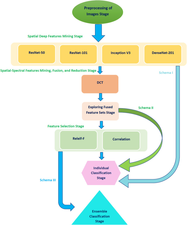
This paper presents a computer-aided facial diagnosis called FaceDisNet to automatically diagnose single and multiple diseases from face scans. FaceDisNet consists of seven stages involving preprocessing of the Disease-Specific Face (DSF) images, spatial deep feature mining stage, spatial-spectral feature mining, fusion, and reduction stage, exploring fused feature set stage, feature selection stage, individual classification stage, and ensemble classification stage. Initially, DSF images are resized and augmented. Following, in the second stage, spatial DL features are mined from four CNNs architectures using TL. Next, in the third stage, spatial-spectral features are mined and fused using DCT. DCT is also used to reduce the dimension of the fused spectral-spatial features. Afterward, the feature sets generated in the previous stage are explored to determine the fused feature set which has the highest impact on the performance of FaceDisNet. Following, two feature selection approaches are employed to further reduce the dimension of the spatial-spectral fused feature set selected in the previous stage. In the individual classification stage, three individual classifiers are utilized to classify single and multiple diseases. Finally, in the ensemble classification, an ensemble classifier is created using the stacking method built on the reduced feature sets generated in the feature selection stage. The ensemble classification stage is done as ensemble classifiers usually enhance the classification performance. A block diagram explaining the seven stages of FaceDisNet is shown in Figure 1.
Figure 1.
A block diagram explaining the six stages of FaceDisNet.
Preprocessing of the DSF dataset
The images of the DSF dataset are reshaped to be equal to the size of the input layers of the four CNNs employed in FaceDisNet. These input sizes are 224 × 224 × 3 for ResNet-50, ResNet-101, and DenseNet-201, and 229 × 229 × 3 for the Inception-V3. As mentioned before, the size of the DSF dataset is 350 images which is relatively small for DL and consequently, the training of the CNNs might suffer from overfitting. Therefore, the augmentation process is crucial to solving this problem.38,39 It enlarges the amount of DSF images by several methods. In this paper, the augmentation methods employed are flipping in the x- and y-directions, translation (−30, 30), scaling (0.9, 1.1), and shearing (0, 45) in the x- and y-directions.
Spatial deep feature mining stage
In this stage, TL is applied to modify the four pre-trained CNNs that were formerly trained on the ImageNet dataset to be able to classify single and multiple diseases from face images. The four CNNs include ResNet-50, ResNet-101, DenseNet-201, and Inception V3. Afterward, the CNNs’ output layers are altered to either two in case of identifying one type of disease and distinguishing it from normal faces with no disease or five in case of classifying multiple diseases. Next, some parameters are tuned, which will be discussed later in the parameter adjustment section. Subsequently, these CNNs are trained on the DSF dataset to either detect a single disease or multiple diseases. Finally, spatial deep features are obtained from a specific layer of every CNN utilizing TL. These layers are the "avg_pool" of the Inception-V3, DenseNet-201, and ResNet-50, and “pool5” of ResNet-101. The number of features obtained from these layers is 1920 for DenseNet-201, and 2048 for Inception, ResNet-50, and ResNet-101.
Spatial-spectral feature mining, fusion, and reduction stage
Spatial features generated in the previous stage are fused using DCT to produce spatial-spectral features. DCT is regularly applied to decompose data into primitive spectral elements. It reveals the data as a total of cosine functions fluctuating at separate frequencies. 40 Usually, the DCT is employed to get the DCT coefficients which are split into three groups: low frequency known as (DC coefficient), middle frequency, and high frequency known as (AC coefficients). High frequencies illustrate noise and tiny changes (details). Whereas lower frequencies are related to the brightness scenarios. Conversely, the middle-frequency coefficients include significant illustrations which create the essential construction of the data. The dimension of the DCT coefficient matrix is identical to the input data. 41 The DCT is also used to reduce the dimension of fused features, however, it does not directly lower the size of the features by itself. 41 An additional reduction phase is often done to perform the reduction using zigzag scanning, where certain DCT coefficients are selected to produce feature vectors.
Exploring fused feature sets stage
In this stage, the fused feature sets generated in the previous stage are explored to find the combined spatial-spectral feature set which has the greatest influence on the accuracy of the disease diagnosis. First, spatial-spectral features of each two CNNs are explored. Then, each spatial-spectral feature combination of every three CNNs is examined. Finally, the spatial-spectral features of the four CNNs are investigated. The feature sets elected in this stage for both identifying a single disease or multiple diseases will undergo two feature selection procedures in the next stage.
Feature selection stage
The fused spatial-spectral sets chosen in the previous step are still of large feature dimensions. This large size of the features increases the complexity of the classifier and could lower its classification capacity.42–44 Feature selection is an important step in many medical computer-aided diagnosis systems to lessen the feature space and remove redundant and irrelevant features. Therefore, in this stage, two popular feature selection procedures are employed, including correlation-based feature selection (CFS) and Relief-F (RF) feature selection methods.
CFS is a popular feature selection method that determines the similarity among features. If two variables are correlated, the correlation coefficient index will lie within the range (−1 to 1). Next, if the two variables are uncorrelated, the correlation coefficient index will be close to 0. 45 The features are ranked according to this correlation coefficient.
Relief-F is a well-known FS method that is commonly used in medical classification problems, due to the efficiency and straightforwardness of computation. The Relief-F method was proposed by Kononenko 46 to be used for multiclass, noisy, and incomplete datasets. Its basic idea is to calculate the significance of features based on their capability to differentiate among instances from the same class close to each other in a local neighborhood. This capability is measured by estimating the weight or score for each feature. 47 Those features that have a higher ability to distinguish between different class instances and increase the distance between them are given higher scores than others that have lower abilities.
Individual classification stage
In this stage, three machine learning classifiers are used individually to perform the classification tasks. These three classifiers involve SVM, Decision Tree (DT), and Naïve Bayes (NB) classifiers. The classification process of FaceDisNet is composed of two categories: binary and multiclass. In the former category, a single disease (beta-thalassemia) is identified and distinguished from normal faces. Whereas in the latter category multiple diseases are classified. Five-fold cross-validation is applied in this paper to validate the results. The individual classification stage is performed in three schemas. In the first schema, the spatial features mined from the four CNNs are used to construct and train the individual classifiers. Schema II uses fused spatial-spectral feature sets to create and learn the individual classifiers. It also explores these feature sets to select the set with the greatest impact on the classification accuracy. Schema III utilizes the spatial spectral features selected using CFS and RF methods to build and learn the three machine classifiers.
Ensemble classification stage
Ensemble classification is a hybrid approach that merges the outputs of several classifiers using a fusion method. It combines the benefits and classification capacity of each classifier in the pool of classifiers, which usually boosts the performance compared to the individual classification. Ensemble classification may prevent the likelihood of achieving inadequate classification results produced by a particular model in the pool. In the medical field, such as diagnosing diseases, ensemble classification corresponds to getting a medical opinion from several doctors to end up with a more convincing medical opinion.48,49 Therefore, ensemble classification is adopted in this paper.
Stacking is a well-known ensemble classification method initially proposed by Wolpert. 50 It involves two classification phases. Phase 0 is known as the base classification. This phase consists of numerous classifiers of different training algorithms. Whereas phase 1 is known as meta-classification, where the predictions of the base classifiers in phase 0 are fused using the meta-classifier of phase 1. In other words, the classification results of the base classifiers along with the class labels are considered as input attributes to the meta-classifier. 51 This meta-classifier is considered the fuser. In this study, an ensemble classification based on stacking is employed, where the base classifiers are SVM, NB, and DT, whereas the meta classifier is an LDA classifier. The ensemble classification using stacking represents schema IV of FaceDisNet.
Experimental setup
Facial disease diagnosis dataset
This study uses a new public dataset called the DSF dataset which can be found in Bo Jin Disease-Specific Faces (2020). 52 This dataset consists of 350 images corresponding to beta-thalassemia, hyperthyroidism, Down syndrome, and leprosy diseases as well as healthy faces. Each of these categories contains 70 images. These images are gathered from medical conferences and meetings, hospitals, specialized medical published articles, and medical websites with specific indicative findings and diagnoses.
Adjustment of CNN’s parameters
To train the four CNNs, numerous network parameters are modified whereas other parameters are left unchanged. These network parameters are the mini-batch size, the number of epochs, the initial learning rate, and the validation frequency. For the binary and multiclass classification categories, the number of epochs is 10, the learning rate is 3 × 10⁻⁴, and the mini-batch size is 10 for each CNN. For the binary classification category, the validation frequency is 24, whereas for the multiclass category it is equal to 61. Stochastic gradient descent with momentum technique is adopted to learn the four CNNs. The four schemas of FaceDisNet are executed using MATLAB 2020 a and Weka Data Mining Tool. 53 The type of processor utilized is Intel(R) Core (TM) i7-10750H, processor frequency of 2.6 GHz, and NVIDIA GeForce GTX 1660 video controller of 6 GB capacity.
Performance metrics
The measures employed to assess the capacity of FaceDisNet in diagnosing single and multiple diseases from face images are explained in this section. The measures are F1-score, sensitivity, precision, accuracy, specificity, and Mathew correlation coefficient (MCC). These measures are computed employing the following mathematical expressions (1–6).
| (1) |
| (2) |
| (3) |
| (4) |
| (5) |
| (6) |
Where the true positive is the number of images that are properly detected by the disease label which they refer to. True negative is the summation of images that do not belong to the detected disease class label and does not refer to. For each disease of the DSF dataset, false positive is the number of images identified as this type of disease, but they do not genuinely refer to it. For every disease of the DSF dataset, false negative is the summation of images not recognized as this disease. The four schemas of FaceDisNet are displayed in Figure 1.
Results and discussions
The results of FaceDisNet are illustrated in this section. FaceDisNet is composed of four schemas, the first three belong to the classification using individual classifiers, whereas the last schema belongs to the ensemble classification. Schema I represents the extraction of spatial features from the four CNNs utilized in FaceDisNet and using these features to train the three individual classifiers. Schema II corresponds to the mining of spatial-spectral features and combining them using DCT and then utilizing these features to learn the three individual classifiers. This schema also searches for the fused spatial-spectral feature sets which have the highest impact on the performance of the classification process. In the third schema, CFS and RF feature selection methods are applied to the feature set selected in the previous schema to reduce the dimension of feature space. These reduced features are then used to construct and train the three individual classifiers. Finally, in the last schema, the reduced features of the earlier schema are used to learn the stacking ensemble classifier.
Schema results
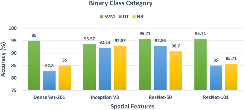
The results of the binary class classification category are first discussed in this subsection. As mentioned before, the binary class category corresponds to identifying one type of disease which is beta-thalassemia and discriminating it from healthy patients with normal faces. Figure 2 shows the binary class accuracy of the three classifiers trained on the spatial features extracted from the four CNNs. It can be noticed from Figure 2 that the SVM classifier has the highest accuracy for the spatial features of the four CNNs. This is obvious as the accuracy is 95%, 93.57%, 95.71%, and 95.71% for the spatial features of DenseNet-201, Inception V3, ResNet-50, and ResNet-101. Followed by the NB classifier which achieves an accuracy of 85%, 92.35%, 90.7%, and 85.71% which is higher than the 82.8%, 92.14%, 92.86%, and 85% attained by the DT classifier trained with the spatial features of DenseNet-201, Inception V3, ResNet-50, and ResNet-101 expect for ResNet-50.
Figure 2.
The classification accuracy of the binary class classification category of the three classifiers trained with the spatial features obtained from the four CNNs. CNNs: convolutional neural networks.
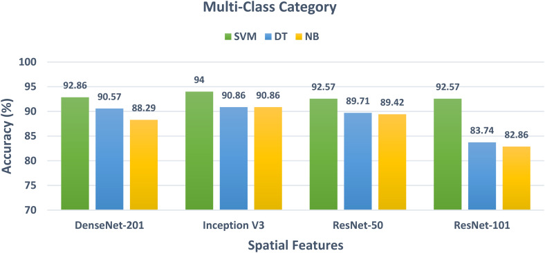
Regarding the multiclass class category which is equivalent to classifying normal and four diseases including beta-thalassemia, hyperthyroidism, Down syndrome, and leprosy, the results displayed in Figure 3 illustrate the multiclass classification accuracy of the three classifiers trained with the spatial features extracted from the four CNNs. Figure 3 indicates that the SVM classifier achieved the greatest accuracy of 92.86%, 94%, 92.57%, and 92.57% by using the spatial features of DenseNet-201, Inception V3, ResNet-50, and ResNet-101. This accuracy is higher than the 90.57%, 90.86%, 89.71%, and 83.74% obtained by the DT classifier and the 88.29%, 90.86%, 89.42%, and 82.86% attained by the NB classifier trained for the spatial features of DenseNet-201, Inception V3, ResNet-50, and ResNet-101, respectively.
Figure 3.
The classification accuracy of the multiclass classification category of the three classifiers trained with the spatial features obtained from the four CNNs. CNNs: convolutional neural networks.
Schema II results
This section shows the results of the spatial-spectral fusion. It explores the performance attained using different combinations of fused feature sets to select the set with the highest performance. The accuracy for the binary class classification category is displayed in Table 2. In the case of fusing every two feature sets, the maximum accuracy of 98.57% is attained by the SVM classifier trained on the spatial-spectral features of ResNet-50 + ResNet-101. This performance is followed by the SVM classifier learned with the spatial-spectral features of Inception + ResNet-101, DenseNet + ResNet-50, DenseNet + Inception, and DenseNet + ResNet-101. Note that the size of the two fused feature sets is 1000 features, which is lower than the 2048 spatial features of Inception V3, ResNet-50, and ResNet-101, and the 1910 spatial features of DenseNet-101 used in the previous schema.
Table 2.
The accuracy (%) achieved for the three classifiers trained with fused spatial-spectral features of the binary class classification category.
| Feature set | SVM | DT | NB |
|---|---|---|---|
| Two spatial-spectral feature sets | |||
| DenseNet + Inception | 95 | 84.28 | 83.57 |
| DenseNet + ResNet-50 | 97.14 | 90.71 | 90.71 |
| DenseNet + ResNet-101 | 95 | 84.28 | 84.28 |
| ResNet-50 + ResNet-101 | 98.57 | 87.14 | 87.14 |
| ResNet-50 + Inception | 95 | 93.57 | 93.57 |
| Inception + ResNet-101 | 97.86 | 86.43 | 86.43 |
| Three spatial-spectral feature sets | |||
| DenseNet + Inception + ResNet-50 | 97.58 | 93.57 | 93.57 |
| DenseNet + Inception + ResNet-101 | 96.43 | 88.57 | 88.57 |
| DenseNet + ResNet-50 + ResNet-101 | 96.43 | 90.71 | 90.71 |
| Inception + ResNet-50 + ResNet-101 | 97.14 | 90.71 | 90.71 |
| Four spatial-spectral feature set | |||
| DenseNet + Inception + ResNet-50 + ResNet-101 | 96.43 | 92.14 | 92.14 |
On the other hand, by fusing each three feature sets, the maximum performance (97.58% accuracy) is attained with the SVM classifier trained on the spatial-spectral features of DenseNet + Inception + ResNet-50. The next higher performance is reached by the SVM classifier (97.14% accuracy) learned utilizing the spatial-spectral features of Inception + ResNet-50 + ResNet-101. Following this performance is the 96.43% accuracy obtained using the SVM classifier trained on the spatial-spectral features of DenseNet + Inception + ResNet-101 as well as DenseNet + ResNet-50 + ResNet-101. The size of the spatial-spectral features of DenseNet + Inception + ResNet-50 which obtained the highest performance (in the case of three feature sets fusion) is 2000, which is lesser than the 2048 spatial features of Inception V3, ResNet-50, and ResNet-101, and slightly higher than the 1910 spatial features of DenseNet-101 used in the previous schema but with higher performance.
Regarding the fusion of the four spatial-spectral features, it can be noticed that the accuracy reached using this set is 96.43%, 92.14%, and 92.14% for the SVM, DT, and NB classifiers, respectively. It can be concluded from Table 1 that the classifiers trained with the spatial-spectral feature have higher performance than that of the spatial feature of schema I. This proves that the fusion using DCT has improved the performance of these classifiers. DCT also has successfully boosted the accuracy with a lower feature size than that obtained by the spatial features of schema I. We can also conclude from Table 2 that the feature set which has the highest accuracy among all fused spatial-spectral feature sets is the ResNet-50 + ResNet-101 which has a feature size of 1000 features and an accuracy of 98.57%. This set will be used in the next schema, which further reduces the feature set dimension by applying the CFS and RF feature selection methods.
The results of schema II in the case of multiclass classification categories are shown in Table 3. It is clear from the results of that table that the SVM classifier obtains the highest performance compared to the NB and DT classifiers. First, for exploring each two fused spatial-spectral features, the peak accuracy of 96.29% is achieved using the SVM classifier constructed with ResNet-50 + Inception, followed by 95.14% of DenseNet + ResNet-101, 94.86% of DenseNet + Inception, 94.57% of DenseNet + ResNet-50, 94.23% Inception + ResNet-101, and 94% of ResNet-50 + ResNet-101. The size of the ResNet-50 + Inception spatial-spectral feature set is 1000, which is smaller than the 2048 spatial feature size of Inception V3, ResNet-50, and ResNet-101, and the 1910 spatial feature size of DenseNet-101 employed in the preceding schema.
Table 3.
The accuracy (%) achieved for the three classifiers trained with fused spatial-spectral features of the multiclass classification category.
| Feature set | SVM | DT | NB |
|---|---|---|---|
| Two spatial-spectral feature sets | |||
| DenseNet + Inception | 94.86 | 93.15 | 93.14 |
| DenseNet + ResNet-50 | 94.57 | 93.43 | 93.43 |
| DenseNet + ResNet-101 | 95.14 | 91.7 | 91.7 |
| ResNet-50 + ResNet-101 | 94 | 89.14 | 88.86 |
| ResNet-50 + Inception | 96.29 | 92 | 92 |
| Inception + ResNet-101 | 94.23 | 89.7 | 89.7 |
| Three spatial-spectral feature sets | |||
| DenseNet + Inception + ResNet-50 | 96.86 | 94 | 94 |
| DenseNet + Inception + ResNet-101 | 96.29 | 93.43 | 93.43 |
| DenseNet + ResNet-50 + ResNet-101 | 96.57 | 93.71 | 93.71 |
| Inception + ResNet-50 + ResNet-101 | 95.71 | 91.4 | 91.4 |
| Four spatial-spectral feature set | |||
| DenseNet + Inception + ResNet-50 + ResNet-101 | 96.29 | 94 | 94 |
In the case of fusing three spatial-spectral features similarly, the SVM classifier attains the greatest accuracy among the other two classifiers. The spatial-spectral features of DenseNet + Inception + ResNet-50 achieve the greatest accuracy of 96.86% using the SVM classifier. Following is the 96.57% accuracy of DenseNet + ResNet-50 + ResNet-101, 96.29% accuracy of DenseNet + Inception + ResNet-101, and the 95.71% accuracy of Inception + ResNet-50 + ResNet-101. On the other hand, when fusing the four spatial-spectral features of DenseNet + Inception + ResNet-50 + ResNet-101, the accuracy reached is 96.29%, 94%, and 94% for the SVM, DT, and NB classifiers respectively.
It is obvious from the results of Table 3 that the classification accuracy has increased when the classifiers are trained with the spatial-spectral feature instead of the spatial features of schema I. This improvement verifies that combining spatial features using DCT has a positive influence on the performance of these classifiers. The fusion process using DCT has also lowered the number of features while increasing the accuracy compared to the spatial features of schema I. Table 3 as well indicates that the maximum accuracy among all combined spatial-spectral feature sets is the DenseNet + Inception + ResNet-50 with a dimension of 2000 features and an accuracy of 96.89%. The spatial-spectral features of DenseNet + Inception + ResNet-50 will be utilized in the subsequent schema to further lower their dimension by employing the CFS and RF feature selection processes.
Schema III results
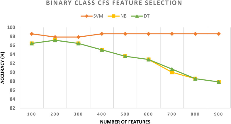
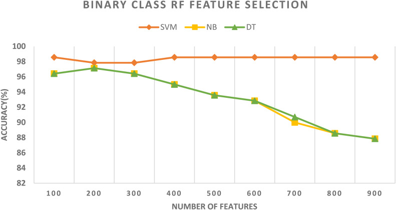
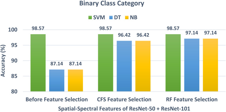
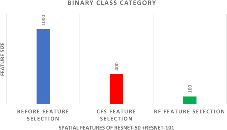
In schema III, the CFS and RF feature selection methods are utilized to further reduce the size of features selected in schema II. For the binary class classification category, the spatial-spectral features of ResNet-50 + ResNet-101 are selected and used to apply the two feature selection methods to them. The binary class classification accuracy of the three classifiers trained with spatial-spectral features of ResNet-50 + ResNet-101 versus the number of features selected for CFS and RF methods are shown in Figures 4 and 5, respectively. Figure 4 shows that the highest accuracy is achieved using the SVM classifier trained with 400 features selected using the CFS method. Whereas Figure 5 shows that the highest accuracy is attained using the SVM classifier trained with 100 features chosen via the RF feature selection method. The binary class classification accuracy of the three classifiers trained with spatial-spectral features of ResNet-50 + ResNet-101 before and after the two feature selection methods are shown in Figure 6. The sizes of the spatial-spectral features of ResNet-50 + ResNet-101 before and after the two feature selection methods are shown in Figure 7 (binary class category). Figure 6 shows that the accuracy of both DT and NB classifiers has been enhanced after using the two feature selection approaches. This is because the accuracies of DT and NB before feature selection are 87.14% and 87.14%, respectively, and equal to (96.42%, 96.42%) and (97.14%, 97.14%) after both CFS and RF feature selection methods. Figure 6 also indicates that the accuracy obtained using the SVM classifier is the same after using the CFS and RF feature selection techniques, however, the number of features has been reduced from 1000 (before FS) to 100 and 400 utilizing RF and CFS feature selection methods, respectively, as shown in Figure 7.
Figure 4.
The binary class classification accuracy of the three classifiers trained with spatial-spectral features of ResNet-50 + ResNet-101 versus the number of features selected using the CFS method. CFS: correlation-based feature selection.
Figure 5.
The binary class classification accuracy of the three classifiers trained with spatial-spectral features of ResNet-50 + ResNet-101 versus the number of features selected using the RF method.
Figure 6.
The binary class classification accuracy of the three classifiers trained with spatial-spectral features of ResNet-50 + ResNet-101 before and after the two feature selection methods.
Figure 7.
The size of features of the spatial-spectral features of ResNet-50 + ResNet-101 before and after the two feature selection methods for the SVM classifier of binary class classification category. SVM: support vector machine.
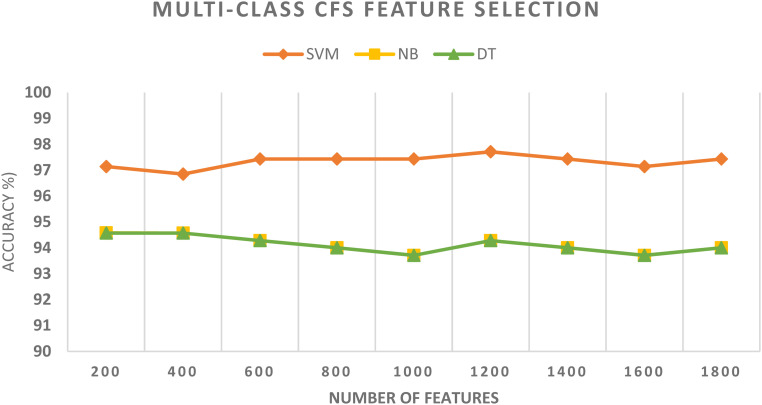
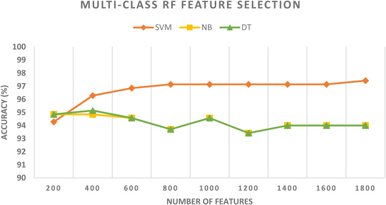
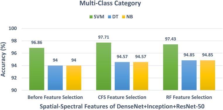
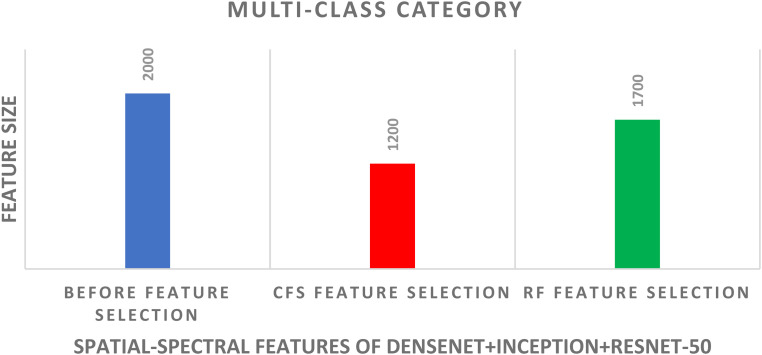
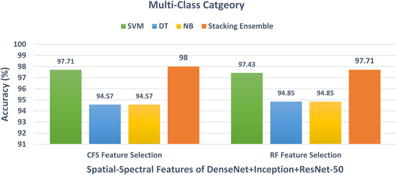
For the multiclass classification category, the spatial-spectral features of DenseNet + Inception + ResNet-50 are chosen in the earlier schema and employed in schema III to further lower their size using CFS and RF methods. The multiclass classification accuracy of the three classifiers learned with the spatial-spectral features of DenseNet + Inception + ResNet-50 versus the number of features selected using CFS and RF feature selection methods are shown in Figures 8 and 9. For the SVM classifier, Figure 8 indicates that the peak accuracy is reached using 1200 features selected via the CFS method. While the maximum accuracy for the SVM classifier is attained utilizing 1700 features chosen using the RF method as displayed in Figure 9. The multiclass classification accuracy of the three classifiers learned with the spatial-spectral features of DenseNet + Inception + ResNet-50 before and after the two feature selection methods are shown in Figure 10. The sizes of the spatial-spectral features of DenseNet + Inception + ResNet-50 before and after the two feature selection methods for the multiclass category are shown in Figure 11. Figure 10 shows that the classification accuracy of the SVM classifier after the RF (97.43%) and CFS (97.71%) feature selection methods has been increased compared to the 96.86% of the SVM classifier achieved before feature selection but the number of features has been reduced to 1200 (CFS method) and 1700 (RF method) instead of the 2000 features utilized before feature selection as shown in Figure 11. Similarly, the accuracies achieved using the DT and NB classifiers are 94.57% and 94.57% after the CFS method, which are higher than the 94% and 94% attained using the same classifiers before feature selection. On the other hand, the accuracies obtained utilizing the DT and NB classifiers after the RF method are 94.85% and 94.85%, which are greater than that attained using the same classifiers before feature selection but with fewer number of features.
Figure 8.
The multi-class classification accuracy of the three classifiers trained with spatial-spectral features of DenseNet + Inception + ResNet-50 versus the number of features selected using the CFS method. CFS: correlation-based feature selection.
Figure 9.
The multi-class classification accuracy of the three classifiers trained with spatial-spectral features of DenseNet + Inception + ResNet-50 versus the number of features selected using the RF method.
Figure 10.
The multi-class classification accuracy of the three classifiers trained with spatial-spectral features of DenseNet + Inception + ResNet-50 before and after the two feature selection methods.
Figure 11.
The size of features of the spatial-spectral features of denseNet + inception + resNet-50 before and after the two feature selection methods for the SVM classifier of the multiclass classification category. SVM: support vector machine.
Schema IV results
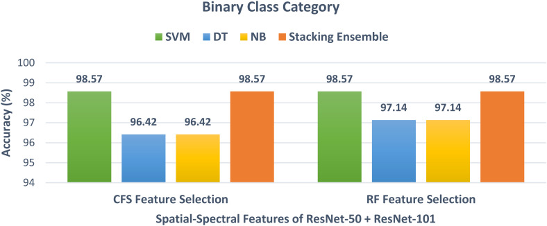
The results after the construction of the stacking ensemble classifier for both binary and multiclass classification categories are discussed in this section. Initially, for the binary class category, the spatial-spectral features of ResNet-50 + ResNet-101 reduced using the CFS and RF feature selection methods in Scheme III are used to train the stacking ensemble classifier. The binary class classification accuracy of the stacking ensemble classifier and the three individual classifiers trained with spatial-spectral features of ResNet-50 + ResNet-101 after the two feature selection methods are demonstrated in Figure 12. It is clear from Figure 12, that the stacking ensemble classifier has an accuracy of 98.57%, which is higher than the 96.42% and 97.14% obtained using the DT and NB classifiers trained on the spatial-spectral features of ResNet-50 + ResNet-101 after CFS and RF feature selection methods, but the same accuracy as the SVM classifier trained with the same features. Figure 13 illustrates the multiclass classification accuracy of the stacking ensemble classifier and the three individual classifiers trained on the spatial-spectral features of DenseNet + Inception + ResNet-50 after the two feature selection methods. The power of the stacking ensemble classifier appears clearly in the multiclass category. This is because Figure 13 shows that the stacking ensemble classifier trained on the spatial-spectral features of DenseNet + Inception + ResNet-50 after RF and CFS methods has achieved an accuracy of 97.71% and 98%. These accuracies are higher than the 97.71% and 97.43% of the SVM after the CFS and RF methods, and the 94.57% and 94.57% of the DT and NB after the CFS method as well as 94.85% and 94.85% of the DT and NB after the RF approach.
Figure 12.
The binary class classification accuracy of the stacking ensemble method and the three classifiers trained with spatial-spectral features of ResNet-50 + ResNet-101 after the two feature selection methods.
Figure 13.
The multi-class classification accuracy of the stacking ensemble method and the three classifiers trained with spatial spectral features of DenseNet + Inception + ResNet-50 after the two feature selection methods.
The performance metrics achieved for the stacking ensemble classifier trained on the fused spatial-spectral features of schema III after feature selection for the binary and multiclass classification categories are displayed in Table 4. This table shows the sensitivity of 0.986, specificity of 0.996, and precision of 0.986. F1 score of 0.986 and MCC of 0.972 are attained using the reduced spatial-spectral features of ResNet-50 + ResNet-101 for both the CFS and RF methods. On the other hand, for the multiclass category, the sensitivity of 0.977, specificity of 0.994, the precision of 0.977, F1-score of 0.977, and MCC of 0.972 are accomplished using the reduced spatial-spectral features of DenseNet + Inception + ResNet-50 after the RF method. Whereas the sensitivity of 0.98, specificity of 0.995, and precision of 0.98. F1-score of 0.98 and MCC of 0.975 are accomplished using the reduced spatial-spectral features of DenseNet + Inception + ResNet-50 after the CFS method.
Table 4.
The performance metrics achieved for the stacking of the ensemble classifier trained with fused spatial-spectral features of schema III after feature selection for the binary and multiclass classification categories.
| Feature selection approach | Sensitivity | Specificity | Precision | F1-Score | MCC |
|---|---|---|---|---|---|
| Binary class category | |||||
| CFS | 0.986 | 0.996 | 0.986 | 0.986 | 0.972 |
| RF | 0.986 | 0.996 | 0.986 | 0.986 | 0.972 |
| Multi-class category | |||||
| CFS | 0.98 | 0.995 | 0.98 | 0.98 | 0.975 |
| RF | 0.977 | 0.994 | 0.977 | 0.977 | 0.972 |
For any medical diagnostic system to be reliable, its specificity and precision should exceed 0.95, and its sensitivity must exceed 0.85.54, 55 The performance metrics of both classification categories of FaceDisNet shown in Table 3 prove that it is a reliable system as the sensitivity for the binary class category is much greater than 0.85, and the specificity and precision are higher than 0.95 for CFS and RF feature selection methods. Likewise, in the multiclass category, the sensitivity is considerably larger than 0.85, and the specificity and precision are greater than 0.95 for CFS and RF feature selection methods. Therefore, FaceDisNet can be believed as a reliable computer-aided facial diagnosis system that may be utilized for the automatic diagnosis of multiple diseases from face images with high accuracy.
Comparison with other methods
The performance of FaceDisNet is also compared with a related computer-aided facial diagnosis system and the state-of-the-art DL model based on the same dataset. The results of this comparison are illustrated in Tables 5 and 6. It can be concluded from Table 5 that FaceDisNet has higher performance compared to that achieved using ResNet-50 + SVM and VGG-16 + SVM 22 for both classification categories. This is due to several reasons, first, methods employed in Jin et al. 22 depend on only spatial features, while FaceDisNet extracts spatial-spectral features to perform classification. Second, techniques utilized in Jin et al. 22 rely on using an individual type of features extracted from CNNs and used distinctly to train an SVM classifier, however, FaceDisNet combines several spatial-spectral features using DCT and searches for the best set of fused features which boots its performance. Third, the methods in Jin et al. 22 did not use any feature selection technique to reduce the feature space dimension and remove unimportant features, which usually enhance the classification performance, whereas FaceDisNet employs two feature selection methods to delete unnecessary features and improve the classification accuracy. Finally, approaches applied in Jin et al. 22 utilized individual classifiers to perform classification, conversely, FaceDisNet utilizes a stacking ensemble classifier to accomplish classification. The competing performance of FaceDisNet enables it to be used for classifying multiple diseases from face images accurately and automatically and reliably.
Table 5.
A comparison between the performance of FaceDisNet and a related computer-aided facial diagnosis system based on the same dataset.
| Model | Sensitivity | Specificity | Precision | F1-Score | Accuracy |
|---|---|---|---|---|---|
| Binary class category | |||||
| ResNet-50 + SVM 22 | 0.9 | 0.932 | 0.931 | 0.915 | 91.7% |
| VGG-16 + SVM 22 | 1 | 0.9 | 0.909 | 0.952 | 95% |
| FaceDisNet | 0.986 | 0.996 | 0.986 | 0.986 | 98.57% |
| Multi-class category | |||||
| ResNet-50 + SVM 22 | - | - | - | - | 92.7% |
| VGG-16 + SVM 22 | - | - | - | - | 93.3% |
| FaceDisNet | 0.98 | 0.995 | 0.98 | 0.98 | 98% |
Table 6.
A comparison between the accuracy (%) of FaceDisNet and the state-of-the-art DL models based on the same dataset.
Table 6 proves that FaceDisNet has an outstanding performance compared to end-to-end pretrained CNNs for both classification categories. As for the binary classification category, the accuracy attained by FaceDisNet is 98.57%, which is higher than the 90.48%, 85.71, 85.7%, and 78.57% accuracy of ResNet-101, ResNet-50, DenseNet-201, and Inception-V3 CNNs, respectively. Similarly, in the multiclass category, the accuracy obtained by FaceDisNet is 98%, which is greater than the 81%, 81%, 80%, and 80% accuracies of ResNet-101, ResNet-50, DenseNet-201, and Inception-V3 CNNs.
Despite the optimistic outcomes that are concluded in the proposed work, this study has a number of limitations. The first problem is that the DL of several hyperparameters requires huge training/validation samples, which are typically insufficient. Furthermore, DL hyperparameter optimization methodologies were not examined.
In addition, the study did not investigate the influence of face manipulation 59 which could possibly affect the performance of the proposed tool. Moreover, another aspect like facial gaining 60 was not explored. People's faces vary dramatically over time, which introduces considerable intraclass variability and makes facial diagnosis a difficult task. Facial disguise is another factor that was not considered in this study. Disguise Invariant Face diagnosis and recognition remain difficult tasks because of the difficulty in identifying and diagnosing faces when their appearances have been intentionally or accidentally altered. Face disguises, whether deliberate or inadvertent, have a significant impact on the diagnostic accuracy and performance of a face recognition system. This is further subdivided into makeup-based facial disguise, accessories-based facial disguise, and a combination of makeup and accessories that affects the facial features, complicating classification for the recognition and diagnosis system. Face cosmetics can be used to add synthetic colors and shading, adjust the size or symmetry of facial features like the lips and eyes, and affect the skin's tone and contours. The challenges for face identification and facial diagnostic systems are further exacerbated by the shifting societal makeup trends. 61 Likewise, wearing glasses, a cap, a scarf, an artificial beard, hair, or moustache obscures some facial features, leading to inaccurate recognition and diagnosis. Thus, face disguises would possibly lower the performance of FaceDisNet.
Conclusions
Many recent studies have demonstrated that a computer-aided facial diagnosis is a promising tool for diagnosing and screening disease from face images. However, most of them were made for identifying a single type of disease in a controlled environment. Many of them have several drawbacks and limitations which avoid them from being used in real-world applications. This study proposed a new computer-aided facial diagnosis system to classify single and multiple diseases from face images called FaceDisNet in an unconstrained environment. It prevented and overcame the drawbacks and limitations of previous studies to be able to be used in real-world applications. FaceDisNet consists of four schemas. The results of schema II showed that spatial-spectral features can enhance the performance of classification compared to the spatial features of schema I. They also proved that feature fusion of features extracted from CNNs of different structures is better than using one type of spatial deep feature. The feature selection procedures of schema III verified their capacity in enhancing the performance of FaceDisNet and removing irrelevant features, thus lowering the dimension of feature space. The ensemble classifier based on stacking constructed in schema IV confirmed its capability in boosting the classification accuracy compared to the previous schemas, especially in the case of diagnosing multiple diseases. The results of FaceDisNet showed its capability in diagnosing single and multiple diseases accurately and automatically using images taken from uncontrolled environments and without the need to detect and segment faces. The outperformance of FaceDisNet compared to other computer-aided facial diagnosis systems proved its ability to be used in real-world scenarios which consequently could prevent disease progression and health complications as well as choosing suitable treatment and follow-up procedures. FaceDisNet can also avoid the misdiagnosis caused by the manual diagnosis as well as the difficulties patients experience in undergoing a medical examination in rural areas. Moreover, it will avoid direct contact between the patient and physicians, especially in the current pandemic of COVID-19. This study may be considered a primary solution to diagnose several diseases in the era of the COVID-19 pandemic. It can open the path for more research concerning an automated solution to medical diagnosis without the need for physical contact between doctors and patients. Upcoming work will concentrate on using more DL techniques. Moreover, collecting more images related to multiple diseases. Factors like face manipulation, facial age, and disguise will be considered in the upcoming work when collecting a new dataset. In addition, the new dataset will include more images of each category of the disease. Furthermore, hyperparameter optimization techniques will be examined in future work.
Footnotes
Author contributions: It is a single-author paper.
Declaration of Conflicting Interests: The author declared no potential conflicts of interest with respect to the research, authorship, and/or publication of this article.
Funding: The author received no financial support for the research, authorship, and/or publication of this article.
ORCID iD: Omneya Attallah https://orcid.org/0000-0002-2657-2264
Guarantor: The author Omneya Attallah will be the guarantor of this manuscript.
Peer review: xxxxxxx.
References
- 1.Wu D, Chen Y, Xu Cet al. et al. Characteristic face: a key indicator for direct diagnosis of 22q11. 2 deletions in Chinese velocardiofacial syndrome patients. PLoS One 2013; 8: e54404. [DOI] [PMC free article] [PubMed] [Google Scholar]
- 2.Fanghänel J, Gedrange T, Proff P. The face-physiognomic expressiveness and human identity. Annals of Anatomy-Anatomischer Anzeiger 2006; 188: 261–266. [DOI] [PubMed] [Google Scholar]
- 3.Delgadillo V, Maria del Mar O, Gort Let al. et al. Natural history of Sanfilippo syndrome in Spain. Orphanet J Rare Dis 2013; 8: 1–11. [DOI] [PMC free article] [PubMed] [Google Scholar]
- 4.Valentine M, Bihm DC, Wolf Let al. Computer-aided recognition of facial attributes for fetal alcohol spectrum disorders. Pediatrics 2017; 140: 2016–2028. [DOI] [PMC free article] [PubMed] [Google Scholar]
- 5.Gripp KW, Baker L, Telegrafi Aet al. et al. The role of objective facial analysis using FDNA in making diagnoses following whole exome analysis. Report of two patients with mutations in the BAF complex genes. American Journal of Medical Genetics Part A 2016; 170: 1754–1762. [DOI] [PubMed] [Google Scholar]
- 6.Attallah O, Ma X. Bayesian neural network approach for determining the risk of re-intervention after endovascular aortic aneurysm repair. Proceedings of the Institution of Mechanical Engineers, Part H: Journal of Engineering in Medicine 2014; 228: 857–866. [DOI] [PubMed] [Google Scholar]
- 7.Karthikesalingam A, Attallah O, Ma Xet al. An artificial neural network stratifies the risks of reintervention and mortality after endovascular aneurysm repair; a retrospective observational study. PloS one 2015; 10: e0129024. [DOI] [PMC free article] [PubMed] [Google Scholar]
- 8.Attallah O. MB-AI-His: histopathological diagnosis of pediatric medulloblastoma and its subtypes via AI. Diagnostics 2021; 11: 359–384. [DOI] [PMC free article] [PubMed] [Google Scholar]
- 9.Attallah O, Sharkas MA, Gadelkarim H. Fetal brain abnormality classification from MRI images of different gestational age. Brain Sci 2019; 9: 231–252. [DOI] [PMC free article] [PubMed] [Google Scholar]
- 10.Attallah O. CoMB-Deep: composite deep learning-based pipeline for classifying childhood medulloblastoma and its classes. Front Neuroinform 2021; 15: 663592. [DOI] [PMC free article] [PubMed] [Google Scholar]
- 11.Attallah O, Zaghlool S. AI-based pipeline for classifying pediatric medulloblastoma using histopathological and textural images. Life 2022; 12: 232. [DOI] [PMC free article] [PubMed] [Google Scholar]
- 12.Ragab DA, Attallah O. FUSI-CAD: coronavirus (COVID-19) diagnosis based on the fusion of CNNs and handcrafted features. PeerJ Computer Science 2020; 6: e306. [DOI] [PMC free article] [PubMed] [Google Scholar]
- 13.Attallah O. ECG-BiCoNet: An ECG-based pipeline for COVID-19 diagnosis using bi-layers of deep features integration. Comput Biol Med 2022; 105210: 1–12. [DOI] [PMC free article] [PubMed] [Google Scholar]
- 14.Attallah O, Samir A. A wavelet-based deep learning pipeline for efficient COVID-19 diagnosis via CT slices. Appl Soft Comput 2022; 109401: 1–16. [DOI] [PMC free article] [PubMed] [Google Scholar]
- 15.Attallah O. An intelligent ECG-based tool for diagnosing COVID-19 via ensemble deep learning techniques. Biosensors 2022; 12: 299. [DOI] [PMC free article] [PubMed] [Google Scholar]
- 16.Attallah O. A computer-aided diagnostic framework for coronavirus diagnosis using texture-based radiomics images. Digital Health 2022; 8: 20552076221092544. [DOI] [PMC free article] [PubMed] [Google Scholar]
- 17.Attallah O, Sharkas M. GASTRO-CADx: a three stages framework for diagnosing gastrointestinal diseases. PeerJ Computer Science 2021; 7: e423. [DOI] [PMC free article] [PubMed] [Google Scholar]
- 18.Anwar F, Attallah O, Ghanem Net al. et al. Automatic breast cancer classification from histopathological images. In: Proceedings of the 2019 International Conference on Advances in the Emerging Computing Technologies (AECT), 2020, pp.1–6: IEEE. [Google Scholar]
- 19.Attallah O, Anwar F, Ghanem NMet al. et al. Histo-CADx: duo cascaded fusion stages for breast cancer diagnosis from histopathological images. PeerJ Computer Science 2021; 7: e493. [DOI] [PMC free article] [PubMed] [Google Scholar]
- 20.Attallah O, Sharkas M. Intelligent dermatologist tool for classifying multiple skin cancer subtypes by incorporating manifold radiomics features categories. Contrast Media Mol Imaging 2021; 2021: 1–14. [DOI] [PMC free article] [PubMed] [Google Scholar]
- 21.Attallah O. DIAROP: automated deep learning-based diagnostic tool for retinopathy of prematurity. Diagnostics 2021; 11: 2034. [DOI] [PMC free article] [PubMed] [Google Scholar]
- 22.Jin B, Cruz L, Goncalves N. Deep facial diagnosis: deep transfer learning from face recognition to facial diagnosis. IEEE Access 2020; 8: 123649–123661. [Google Scholar]
- 23.Basel-Vanagaite L, Wolf L, Orin Met al. et al. Recognition of the Cornelia de Lange syndrome phenotype with facial dysmorphology novel analysis. Clin Genet 2016; 89: 557–563. [DOI] [PubMed] [Google Scholar]
- 24.Hadj-Rabia S, Schneider H, Navarro Eet al. Automatic recognition of the XLHED phenotype from facial images. American Journal of Medical Genetics Part A 2017; 173: 2408–2414. [DOI] [PubMed] [Google Scholar]
- 25.Vieira S, Pinaya WH, Mechelli A. Using deep learning to investigate the neuroimaging correlates of psychiatric and neurological disorders: methods and applications. Neurosci Biobehav Rev 2017; 74: 58–75. [DOI] [PubMed] [Google Scholar]
- 26.Kong X, Gong S, Su Let al. et al. Automatic detection of acromegaly from facial photographs using machine learning methods. EBioMedicine 2018; 27: 94–102. [DOI] [PMC free article] [PubMed] [Google Scholar]
- 27.Schneider HJ, Kosilek RP, Günther Met al. A novel approach to the detection of acromegaly: accuracy of diagnosis by automatic face classification. J Clin Endocrinol Metab 2011; 96: 2074–2080. [DOI] [PubMed] [Google Scholar]
- 28.Meng T, Guo X, Lian Wet al. Identifying facial features and predicting patients of acromegaly using three-dimensional imaging techniques and machine learning. Front Endocrinol (Lausanne) 2020; 11: 492. [DOI] [PMC free article] [PubMed] [Google Scholar]
- 29.Zhao Q, Rosenbaum K, Sze Ret al. et al. Down Syndrome Detection from Facial Photographs Using Machine Learning Techniques. In Proceedings of the Medical Imaging 2013: Computer-Aided Diagnosis; International Society for Optics and Photonics, 2013; Vol. 8670, p. 867003.
- 30.Zhao Q, Okada K, Rosenbaum Ket al. et al. Hierarchical Constrained Local Model Using ICA and Its Application to Down Syndrome Detection. In Proceedings of the International Conference on Medical Image Computing and Computer-Assisted Intervention; Springer, 2013; pp. 222–229. [DOI] [PubMed]
- 31.Zhao Q, Okada K, Rosenbaum Ket al. et al. Digital facial dysmorphology for genetic screening: hierarchical constrained local model using ICA. Med Image Anal 2014; 18: 699–710. [DOI] [PubMed] [Google Scholar]
- 32.Liu W, Li M, Yi L. Identifying children with autism spectrum disorder based on their face processing abnormality: a machine learning framework. Autism Res 2016; 9: 888–898. [DOI] [PubMed] [Google Scholar]
- 33.Wang K, Luo J. Detecting visually observable disease symptoms from faces. EURASIP Journal on Bioinformatics and Systems Biology 2016; 2016: 1–8. [DOI] [PMC free article] [PubMed] [Google Scholar]
- 34.Sajid M, Shafique T, Baig MJAet al. et al. Automatic grading of palsy using asymmetrical facial features: a study complemented by new solutions. Symmetry (Basel) 2018; 10: 242. [Google Scholar]
- 35.Guo Z, Li W, Dai Jet al. et al. Facial imaging and landmark detection technique for objective assessment of unilateral peripheral facial paralysis. Enterprise Information Systems 2021: 1–17. [Google Scholar]
- 36.Gurovich Y, Hanani Y, Bar Oet al. Identifying facial phenotypes of genetic disorders using deep learning. Nat Med 2019; 25: 60–64. [DOI] [PubMed] [Google Scholar]
- 37.Pantel JT, Hajjir N, Danyel Met al. Efficiency of computer-aided facial phenotyping (DeepGestalt) in individuals with and without a genetic syndrome: diagnostic accuracy study. J Med Internet Res 2020; 22: e19263. [DOI] [PMC free article] [PubMed] [Google Scholar]
- 38.Perez L, Wang J. The effectiveness of data augmentation in image classification using deep learning. arXiv preprint arXiv 2017: 1–8. [Google Scholar]
- 39.Shorten C, Khoshgoftaar TM. A survey on image data augmentation for deep learning. J Big Data 2019; 6: 1–48. [DOI] [PMC free article] [PubMed] [Google Scholar]
- 40.Aydoğdu Ö, Ekinci M. An approach for streaming data feature extraction based on discrete cosine transform and particle swarm optimization. Symmetry (Basel) 2020; 12: 299. [Google Scholar]
- 41.Dabbaghchian S, Ghaemmaghami MP, Aghagolzadeh A. Feature extraction using discrete cosine transform and discrimination power analysis with a face recognition technology. Pattern Recognit 2010; 43: 1431–1440. [Google Scholar]
- 42.Li J, Liu H. Challenges of feature selection for big data analytics. IEEE Intell Syst 2017; 32: 9–15. [Google Scholar]
- 43.Attallah O, Karthikesalingam A, Holt PJet al. et al. Feature selection through validation and un-censoring of endovascular repair survival data for predicting the risk of re-intervention. BMC Med Inform Decis Mak 2017; 17: 115–133. [DOI] [PMC free article] [PubMed] [Google Scholar]
- 44.Attallah O, Karthikesalingam A, Holt PJet al. et al. Using multiple classifiers for predicting the risk of endovascular aortic aneurysm repair re-intervention through hybrid feature selection. Proceedings of the Institution of Mechanical Engineers. Part H: Journal of Engineering in Medicine 2017; 231: 1048–1063. [DOI] [PubMed] [Google Scholar]
- 45.Michalak K, Kwasnicka H. Correlation based feature selection method. International Journal of Bio-Inspired Computation 2010; 2: 319–332. [Google Scholar]
- 46.Kononenko I. Estimating Attributes: Analysis and Extensions of RELIEF. In Proceedings of the European conference on machine learning; Springer, 1994; pp. 171–182.
- 47.Zhang J, Chen M, Zhao Set al. et al. ReliefF-based EEG sensor selection methods for emotion recognition. Sensors 2016; 16: 1558. [DOI] [PMC free article] [PubMed] [Google Scholar]
- 48.Ragab DA, Sharkas M, Attallah O. Breast cancer diagnosis using an efficient CAD system based on multiple classifiers. Diagnostics 2019; 9: 165–190. [DOI] [PMC free article] [PubMed] [Google Scholar]
- 49.Chen H, Xiong W, Wu Jet al. et al. Decision-making model based on ensemble method in auxiliary medical system for non-small cell lung cancer. IEEE Access 2020; 8: 171903–171911. [Google Scholar]
- 50.Wolpert DH. Stacked generalization. Neural Netw 1992; 5: 241–259. [Google Scholar]
- 51.Džeroski S, Ženko B. Is combining classifiers with stacking better than selecting the best one? Mach Learn 2004; 54: 255–273. [Google Scholar]
- 52.Bo Jin Disease-Specific Faces 2020.
- 53.Hall M, Frank E, Holmes Get al. et al. The WEKA data mining software: an update. ACM SIGKDD Explorations Newsletter 2009; 11: 10–18. [Google Scholar]
- 54.Attallah O. An effective mental stress state detection and evaluation system using minimum number of frontal brain electrodes. Diagnostics 2020; 10: 292–327. [DOI] [PMC free article] [PubMed] [Google Scholar]
- 55.Colquhoun D. An investigation of the false discovery rate and the misinterpretation of P-values. R Soc Open Sci 2014; 1: 140216. [DOI] [PMC free article] [PubMed] [Google Scholar]
- 56.Szegedy C, Vanhoucke V, Ioffe Set al. et al. Rethinking the inception architecture for computer vision. In: Proceedings of the IEEE conference on computer vision and pattern recognition, 2016, pp.2818–2826: IEEE. [Google Scholar]
- 57.Huang G, Liu Z, Van Der Maaten Let al. et al. Densely connected convolutional networks. In: Proceedings of the IEEE conference on computer vision and pattern recognition, 2017, pp.4700–4708: IEEE. [Google Scholar]
- 58.He K, Zhang X, Ren Set al. et al. Deep Residual Learning for Image Recognition. In: Proceedings of the IEEE Conference on Computer Vision and Pattern Recognition, 2016. [Google Scholar]
- 59.Rossler A, Cozzolino D, Verdoliva Let al. et al. Faceforensics + +: learning to detect manipulated facial images. In: Proceedings of the IEEE/CVF international conference on computer vision, 2019, pp.1–11. [Google Scholar]
- 60.Yousaf A, Khan MJ, Khan MJet al. et al. A robust and efficient convolutional deep learning framework for age-invariant face recognition. Expert Syst 2020; 37: e12503. [Google Scholar]
- 61.Khan MJ, Khan MJ, Siddiqui AMet al. et al. An automated and efficient convolutional architecture for disguise-invariant face recognition using noise-based data augmentation and deep transfer learning. Vis Comput 2022; 38: 509–523. [Google Scholar]


