Uncertainty estimation strategies for quantitative non-targeted analysis

Abstract

Non-targeted analysis (NTA) methods are widely used for chemical discovery but seldom employed for quantitation due to a lack of robust methods to estimate chemical concentrations with confidence limits. Herein, we present and evaluate new statistical methods for quantitative NTA (qNTA) using high-resolution mass spectrometry (HRMS) data from EPA’s Non-Targeted Analysis Collaborative Trial (ENTACT). Experimental intensities of ENTACT analytes were observed at multiple concentrations using a semi-automated NTA workflow. Chemical concentrations and corresponding confidence limits were first estimated using traditional calibration curves. Two qNTA estimation methods were then implemented using experimental response factor (RF) data (where RF = intensity/concentration). The bounded response factor method used a non-parametric bootstrap procedure to estimate select quantiles of training set RF distributions. Quantile estimates then were applied to test set HRMS intensities to inversely estimate concentrations with confidence limits. The ionization efficiency estimation method restricted the distribution of likely RFs for each analyte using ionization efficiency predictions. Given the intended future use for chemical risk characterization, predicted upper confidence limits (protective values) were compared to known chemical concentrations. Using traditional calibration curves, 95% of upper confidence limits were within ~tenfold of the true concentrations. The error increased to ~60-fold (ESI+) and ~120-fold (ESI−) for the ionization efficiency estimation method and to ~150-fold (ESI+) and ~130-fold (ESI−) for the bounded response factor method. This work demonstrates successful implementation of confidence limit estimation strategies to support qNTA studies and marks a crucial step towards translating NTA data in a risk-based context.

Introduction

Chemical exposures are an unavoidable aspect of life, with thousands of chemicals found in the air we breathe, the food and beverages we ingest, the consumer products we apply, and the buildings we inhabit [1, 2]. The production, use, and disposal of man-made materials introduce new chemicals into a range of matrices, opening new exposure pathways for human and ecological receptors. Given the vast number of pathways and unexplored chemical receptor interactions, it is difficult to assess all possible risk scenarios. A clear need therefore exists for approaches to efficiently evaluate chemical safety across a range of matrices, receptors, and exposure scenarios.

In order to assess the safety of any given chemical, researchers must determine whether the chemical has the potential to cause harm to a population (hazard identification), the exposure level(s) above which harm is expected (dose–response assessment), and the exposure level(s) expected within the population for whom safety is being assessed (exposure assessment) [3]. For nearly a half-century, this risk-based paradigm has influenced research and regulatory institutions that consider the safety of man-made (and naturally occurring) chemicals. In the USA, the Environmental Protection Agency regulates certain chemicals and manages exposures under numerous statutes, including the Toxic Substances Control Act; the Federal Insecticide, Fungicide, and Rodenticide Act; and the Safe Drinking Water Act. Chemical monitoring data (i.e., measurements of chemicals in matrices such as air, water, and soil) are a pillar for each statute, providing a defensible scientific basis for regulatory standards, as well as a means to ensure compliance with those standards.

Targeted analytical methods provide the chemical monitoring data to support regulatory decisions and actions under existing statutes. In the workflows of targeted methods, chemicals of interest are selected, and procedures developed to yield quantitative measures within defined boundaries of accuracy and precision. While recognized as the gold standard for chemical monitoring, targeted methods are bounded by the known; they are designed only to achieve a specified level of performance for pre-defined chemicals of interest. As such, these methods are ill-equipped to anticipate contaminants of emerging concern (CECs), thus leaving potential risks from chemical unknowns as a significant “blind spot.”

Non-targeted analysis (NTA) methods, often employing high-resolution mass spectrometry (HRMS), have proven an effective means of identifying CECs in a wide variety of media, including drinking water [4, 5], food [6], house dust [7–9], soil and sediment [10, 11], consumer products [12, 13], human fluids and tissues [14, 15], and biota [16, 17]. NTA is a burgeoning field for environmental applications, with considerable advancements to hardware, software, databases, and workflows being realized with ever-increasing frequency [18]. With swift advancement comes a growing need for standardization of terms, metrics, benchmarks, and protocols [18, 19]. Most emphasis to date has been placed on the ability of NTA methods to correctly identify compounds in samples of interest [20–22]. Considerably less emphasis has been placed on the ability of NTA methods to quantify concentrations of chemical suspects via the acquired NTA data (i.e., in the absence of follow-up targeted analysis). This imbalance has created a challenge for risk assessors, policy makers, and regulators who would like to consider NTA findings as part of decision-making processes but lack quantitative interpretation strategies.

Due to the emphasis on identification rather than quantification, it is well established that NTA methods are best suited to identify CECs and inform follow-up targeted analyses. This scenario is entirely realistic for the study of chemicals that are commercially available, trivially synthesizable, or otherwise obtainable from manufacturers. Many CECs, however, do not meet these criteria. Options for targeted method development are therefore limited for some chemical discoveries that garner considerable public attention. This scenario encapsulates a fundamental challenge for the NTA research community: how can CECs be provisionally evaluated for health risks in the absence of traditional quantitative estimates ?

The answer to this question lies in the development of quantitative NTA (qNTA) methods. Here, qNTA methods are defined as those that can estimate analyte concentration in the absence of authentic standards. Numerous qNTA methods exist [23–27], with most estimating chemical concentrations based on observed behaviors of surrogate analytes (often selected based on structural similarity or proximity of chromatographic elution time), or model-predicted behaviors of identified analytes. Method performance is generally examined using experimental data for diverse test compounds and post hoc calculations of prediction error (e.g., the average and/or maximum prediction error across a test set). For practical applications, however, it is critical to communicate the degree of uncertainty in specific qNTA predictions. In other words, for real-world use, stakeholders (e.g., the public, elected officials, risk assessors) will wish to know: for any detected CEC, in what range is the true concentration confidently expected to lie?

The concepts of measurement uncertainty are germane to chemical risk assessment but have yet to be fully considered in the context of qNTA. Therefore, we explored qNTA from a fundamental statistical perspective with a focus on communicating study results in such a way that they are informative and actionable. Analytical chemistry and statistical concepts were examined using experimental NTA data from 673 unique chemicals measured as part of EPA’s Non-Targeted Analysis Collaborative Trial (ENTACT) [22, 28]. These measurements were collected using semi-automated data processing techniques as part of a multi-step NTA workflow. Herein we present and discuss (1) key mathematical and experimental assumptions that underlie qNTA studies; (2) the extent to which ENTACT NTA data adhere to these assumptions; (3) a naïve method for generating statistically defensible confidence limits for qNTA estimates; (4) the prediction error incurred when implementing the naïve method; and (5) the extent to which prediction error can be reduced using chemometric modeling approaches.

Background

Quantitative, targeted mass spectrometry experiments determine analyte concentrations through the use of compound-specific calibration curves. A calibration curve is a visual (plot) and mathematical (equation) relationship between the known concentrations of an analyte in prepared solution (independent variable, denoted “Conc”) and the observed instrument responses (dependent variable, denoted “Y_obs”) at the known concentrations. Mathematical parameter estimates that describe the calibration curve (e.g., slope and y-intercept) are ultimately used to estimate concentrations of the target chemical in unknown samples given observed instrument responses in a process known as “inverse prediction.”

When working within the linear dynamic range, a change in analyte concentration is directly proportional to the resulting change in instrument response (compound peak intensity, which may be expressed as an area or height). Figure 1A illustrates two simulated examples of this proportional relationship, where a doubling of the concentration yields a doubling of the observed intensity, and measurements are represented as triplicates with a constant 10% experimental error. For both theoretical chemicals, the quotient of intensity/concentration is constant over the experimental range, mathematically equivalent to the linear regression slope, and termed the compound-specific “response factor” (RF). The linear regression intercept values are located at the graph origin in Fig. 1A, reflecting an instrument response of zero at a known concentration of zero. Since in these two examples the relationships between concentration and intensity are linear and proportional, one needs to only know the RF to estimate concentration $(\widehat{\text{Conc}})$ given an observed intensity (Y_obs) (where $\widehat{Conc}=Y_{obs}/RF$).

Fig. 1.

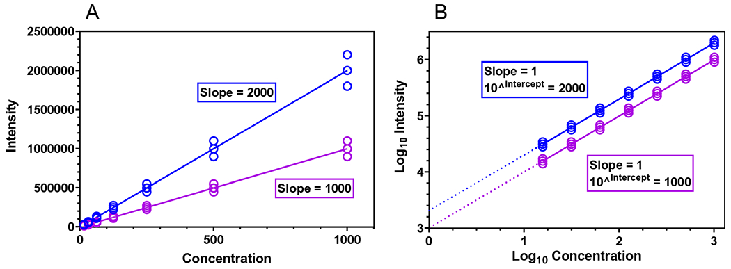
A Two theoretical calibration curves with unequal point spacing on the X axis and heteroscedastic measurement errors (Y axis) about the regression lines. Here, the regression slopes are equal to the chemical-specific response factors (RF = intensity/concentration). B Two theoretical calibration curves, based on the exact data from (A) after base 10 logarithmic transformation. Here, point spacing is equal along the X axis, and measurement error (Y axis) is homoscedastic about the regression line. Furthermore, the slope of each regression line equals one (indicating a perfectly proportional relationship between concentration and intensity), and the intercept equals the chemical-specific RF, after exponentiation

To the discerning analyst, two issues exist with the calibration curves shown in Fig. 1A. First, concentrations used for the calibration curves reflect a dilution series with a common dilution factor (i.e., X axis values are spaced by a factor of two). The use of a common dilution factor leads to unequal spacing of concentration values along the X axis and, in turn, outsized influence of higher concentration data points on estimated regression parameters. Second, while the relative measurement error (often expressed as relative standard deviation [RSD]) is constant across the concentration range, the absolute error in replicate measurements increases with higher concentration values. This phenomenon, known as “heteroscedasticity,” is a violation of a fundamental assumption of least-squares regression. If not addressed, this issue can yield inaccurate confidence and prediction intervals from regressions based on the raw measurement data.

In practice, both of these issues can be overcome using regression weighting strategies or data transformations. As shown in Fig. 1B, logarithmic transformation of concentration and intensity values allows a simple linear regression without violating the regression assumption of homoscedasticity and without biasing the curve fit towards the highest calibration point(s). Specifically, log transformation of the concentration values allows for equally spaced points on the X axis, and log transformation of the intensity values allows for equal error about the regression line across the concentration range. As a result of performing the regression on log-transformed values for concentrations and intensities, the slope of each simulated regression is now exactly one (an ideal case), reflecting the perfectly proportional relationship between concentration and intensity. Given a slope of exactly one, it can be shown (Supporting Information 1.0) that the regression intercept, after exponentiation, is equivalent to the RF. In light of these mathematical properties, log–log calibration curves represent a straightforward method to prepare linear, proportional calibration curves that allow defensible inverse prediction. When slope values are shown to be indistinguishable from 1.0, chemical-specific RFs can be determined using the estimated intercept of the log–log regression equation. However, any deviations from proportionality (where the log–log regression slope does not equal one) require alternative strategies for calculating and interpreting chemical-specific RFs, as shown below.

Methods

Generating an NTA dataset

Data for this this proof-of-concept work was derived from previous analyses performed as part of ENTACT, with specific methods described by Sobus et al. [22] and the overall study design described by Ulrich et al. [28]. Briefly, ENTACT is a large multi-laboratory study designed to assess the state-of-the-science of NTA methods using complex synthetic mixtures, standardized reference materials (i.e., house dust, human serum, and silicone bands), and fortified reference materials. This current study focuses only on the synthetic mixtures (n = 10), which are comprised of 1,269 chemical substances dissolved in organic solvent. Each mixture contains between 95 and 365 chemical substances, with individual substances mapped to MS-Ready structures (Supporting Information 2.0), and certain substances deliberately included in multiple mixtures. The ENTACT mixtures were analyzed using liquid chromatography (LC) quadrupole time-of-flight (Q-TOF) high-resolution mass spectrometry (HRMS). Reverse-phase chromatography was used for compound separation, followed by electrospray ionization in positive (ESI+) and negative (ESI−) modes. Full scan (MS¹) and tandem (MS²) mass spectra were used for compound identification as part of an intricate semi-automated workflow, as described by Sobus et al. [22].

Anticipating future interest in qNTA evaluations, the ENTACT mixtures were examined in triplicate at three dilutions. Each analytical batch included “low,” “mid,” and “high” nominal concentrations of at least one ENTACT mixture (specific chemical concentrations are given in Tables S1 and S2), along with solvent and method blanks. Stable isotope labeled tracer compounds (three in ESI+ ; eight in ESI−) were used to track method performance across all samples and batches. Tracer results showed clear sample (i.e., concentration-dependent) and batch effects and were therefore used to normalize measured abundances for detected ENTACT substances within and between batches (Supporting Information 3.0).

All ENTACT substances observed via semi-automated processing were manually reviewed for quality using extracted ion chromatograms and associated spectra. The final curated results include experimental data for 530 unique compounds (1940 distinct measurements) observed in ESI+ mode (Table S1) and 237 unique compounds (691 distinct measurements) observed in ESI− mode (Table S2). Several spiked substances were observed (by MS-Ready structure) as multiple isomer peaks (with distinct retention times) during automated processing (12 in ESI+ mode and 0 in ESI− mode); intensity values (i.e., peak areas) for related isomer peaks were summed in the final dataset. Some spiked substances were observed by MS-Ready structure across mixtures (73 in ESI+ mode and 10 in ESI− mode); this data subset allowed for a more rigorous evaluation of measurement error effects on inverse predictions (described in section Inverse prediction using calibration curves (CC)).

qNTA evaluation framework

The following sections detail three methods (one traditional quantitation method and two qNTA methods) for generating concentration confidence interval estimates for chemicals observed in an NTA dataset. The purpose of each method is to estimate, given some observed experimental intensity (Y_obs), the range of values containing the true chemical concentration at a defined level of confidence (e.g., 95%). Any of the presented methods can be used to estimate lower and upper confidence limits, with upper-bound estimates being of greatest interest for informing chemical safety assessments, since they represent a conservatively high exposure metric. In other words, a lower confidence limit of a concentration estimate would communicate a lower risk and therefore not suitably protect a target population in a safety assessment. A scheme outlining all three approaches, and their application to the ENTACT data, is shown in Fig. 2.

Fig. 2.

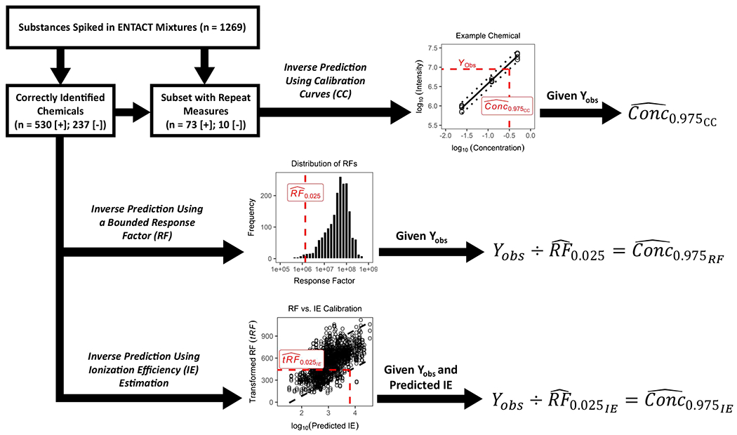
A workflow illustrating the use of ENTACT mixtures data to evaluate concentration estimation methods. The first approach, inverse prediction using calibration curves, follows traditional quantitative procedures and was relevant for only a subset of ENTACT chemicals measured across multiple mixtures. Here, upper-bound concentration estimates $({\widehat{Conc}}_{{0.975}_{CC}})$ were calculated using observed intensities (Y_obs) and compound-specific calibration curves with 95% prediction intervals. The second approach, inverse prediction using a bounded response factor, was applied to all measured ENTACT chemicals, with upper-bound concentration estimates $({\widehat{Conc}}_{{0.975}_{RF}})$ calculated using the 2.5th percentile estimate of a response factor distribution $({\widehat{RF}}_{0.025})$. The third approach, inverse prediction using ionization efficiency estimation, was also applied to all measured ENTACT chemicals. Here, IE was first predicted for each ENTACT chemical using an existing machine learning model. A calibration of RF vs. predicted IE (with appropriate data transformations) then enabled estimation of the upper-bound concentration $({\widehat{Conc}}_{{0.975}_{IE}})$ for each measured ENTACT chemical given Y_obs and predicted IE

The traditional quantitation method involves inverse prediction via calibration curves and requires repeat measures of individual chemicals to establish reliable prediction intervals. For our dataset, calibration curve prediction intervals were generated only for ENTACT compounds measured across multiple mixtures (73 compounds in ESI+ mode and 10 in ESI− mode). All data used for inverse predictions were obtained via semi-automated NTA methods. Measurement precision therefore reflects error incurred from standard NTA data processing procedures (e.g., deconvolution, componentization, alignment, autointegration) and not from targeted ion extraction and manual peak integration. The traditional calibration approach is commonly used for targeted analysis and is therefore the benchmark method against which qNTA methods can be assessed. It is noteworthy, however, that traditional calibration is not viable for actual NTA studies given the need for multi-point calibration data derived from analytical standards of every chemical substance.

Two qNTA methods were applied to the full suite of ENTACT data (530 unique compounds in ESI+ mode and 237 in ESI− mode) (Fig. 2). The first method, considered here as the naïve qNTA model (i.e., not considering molecular descriptors and likely to yield the largest prediction error), makes use of a statistical distribution of chemical-specific RF estimates. Section Inverse prediction using a bounded response factor (RF) describes the assumptions and calculations involved with this bounded response factor method. The second method makes use of chemical ionization efficiency (IE) estimates as predicted from a machine learning algorithm based on molecular descriptors. The assumptions and calculations involved with this ionization efficiency estimation method are described in section Inverse prediction using ionization efficiency (IE) estimation.

Inverse prediction using calibration curves (CC)

All calibration curves were based on linear regression of log₁₀-transformed intensity (Y term) and log₁₀-transformed concentration (X term) values. Data used for regression modeling are given in Tables S1 (ESI+ data) and S2 (ESI− data). Calibration curves were first generated for the subset of ENTACT chemicals measured across multiple mixtures (73 compounds in ESI+ mode and 10 in ESI− mode). For this subset, data for a given chemical were required to be balanced across mixtures (i.e., have the same number of measurements — this was not always the case for all chemicals given some observations being below the limit of detection). This requirement minimized bias in parameter estimates (i.e., slope and y-intercept) and maximized the uniformity of model residuals.

The regression prediction interval was calculated (using the “predict” function within the car R package [Companion to Applied Regression]) [29] for each calibration curve using a 95% confidence level — this interval defines the range in which a future intensity value (Y_obs) would be expected to fall, with 95% confidence, given a new sample analysis at a known concentration. Additional calibration curves were generated for the remainder of the ENTACT chemicals that were measured in only one mixture (but at multiple concentrations) — the purpose for generating these calibration curves was to assess linearity for each measured analyte. Prediction intervals were not calculated for this chemical set because repeated measures were not available for chemicals across mixtures.

Following regression analysis, all observed intensities (Y_obs) for each chemical were used for inverse prediction (using the investr R package) [30] of chemical concentrations. For the subset of chemicals measured across multiple mixtures, two concentration estimates were calculated for each Y_obs. The first estimate, ${\widehat{Conc}}_{CC}$, represents the best estimate of the true concentration and was calculated by solving the regression equation for Conc (independent variable) given Y_obs (with exponentiation required for interpretation of predicted values outside of logarithmic space). This estimate is consistent with the expected result of a traditional targeted method employing a chemical-specific calibration curve. The second estimate, ${\widehat{Conc}}_{{0.975}_{CC}}$, represents the upper confidence limit of the concentration estimate given Y_obs. The upper confidence limit estimate is defined as the abscissa value for which Y_obs intersects the line representing the lower bound of the 95% prediction interval (see Fig. 2, top). For the subset of chemicals measured in only one mixture, only ${\widehat{Conc}}_{CC}$ was determined because prediction interval estimates were not calculated.

Inverse prediction using a bounded response factor (RF)

As previously discussed in the Background section, when working within a linear dynamic range, the RF for an individual chemical is assumed to be constant. Given an observed intensity (Y_obs) for that chemical (within the defined range), the concentration can be quickly estimated $\widehat{Conc}=Y_{obs}/RF$. Under ideal conditions, it is assumed that all measurable chemicals each exhibit a constant RF and that chemical-specific RF values span a distribution of unknown size and shape. In the absence of any additional information, the median of this distribution (RF_0.5) could be applied to any new Y_obs for any new chemical, and the concentration could be estimated as ${\widehat{Conc}}_{{0.5}_{RF}}=Y_{obs}/R{F}_{0.5}$. Accordingly, this calculated value would be equally likely to overestimate or underestimate the true concentration. For purposes of qNTA to support chemical safety evaluations, underestimation of concentration is likely undesirable for any chemical of interest, particularly when having limited knowledge of the magnitude of underestimation. In other cases, such as evaluations of food authenticity, overestimation of chemical concentration may be undesirable. Thus, a preferred qNTA method would yield a concentration estimate with confidence limits given any Y_obs. As a naïve estimation approach, a 95% prediction interval could first be determined for the RF distribution based on 2.5th and 97.5th percentiles estimates (i.e., ${\widehat{RF}}_{0.025}$ and ${\widehat{RF}}_{0.975}$, respectively). Then, when estimating chemical concentration given Y_obs, a lower confidence limit could be estimated as ${\widehat{Conc}}_{{0.025}_{RF}}=Y_{obs}/R{F}_{0.975}$, and an upper confidence limit could be estimated as ${\widehat{Conc}}_{{0.975}_{RF}}=Y_{obs}/R{F}_{0.025}$.

While the RF is theoretically stable for a given analyte on a given instrument (when examined within the linear dynamic range), empirical RF values are influenced by random and/or systematic error. Explicitly considering these errors allows for quantitative evaluation of qNTA methods. The data collected during ENTACT provides an empirically measured, diverse chemical subset on which to develop and test mathematical hypotheses related to qNTA. All ENTACT chemicals were evaluated using multiple concentrations, and some were additionally evaluated using more than one chemical mixture. Given this design, all ENTACT chemicals have multiple empirical RF values (recall that each concentration and intensity pair yields an empirical RF value). In total, 1940 and 691 RF values were available from ESI+ (Table S1) and ESI− (Table S2) analyses, respectively. While the ENTACT chemical set does not represent the entirety of chemical space, it can be considered representative of common commercial chemicals analyzed by LC–MS. To best estimate the 2.5th and 97.5th percentiles of the ENTACT RF distributions (as intended surrogates of a larger chemical space), bootstrap resampling was performed on the ENTACT RF data as part of a fivefold cross-validation procedure. Here, bootstrap resampling helps assess the uncertainty in estimating the 2.5th and 97.5th percentiles from this data set, and fivefold cross-validation helps assess whether the results are generalizable to chemicals outside this data set.

Briefly, each unique chemical (defined by its MS-Ready Distributed Structure-Searchable Toxicity Database Chemical Identifier [MS-Ready DTXCID]) was randomly assigned, without replacement, to one of five subsets (or “folds”). Next, four of the five folds were grouped as a training set, with the remaining fold treated as a test set. The partitioning of training and tests sets was repeated five times such that each fold was once considered as the test set in one of the five iterations of the training and evaluation process.

Each chemical in each training and test set had multiple RF values, ranging from two to 24 per chemical (recall that some compounds were measured in multiple mixtures and some compounds could not be detected at all three nominal spike levels). For each training set, hierarchical bootstrap sampling was performed first by chemical and then by RF value. Specifically, a chemical was first randomly sampled, and then an RF value for that chemical was randomly sampled. All random sampling was performed with replacement. Mirroring the underlying dataset, 530 chemical/RF values were sampled for ESI+ mode, and 237 chemical/RF values were sampled for ESI− mode. The random sampling of chemical/RF values was repeated 10,000 times for each training set. For each of the 10,000 random samples, the 2.5th and 97.5th percentile RF values were determined (using the “quantile” function within the base R “stats” package) [31] and recorded. The medians of these 2.5th and 97.5th percentile estimates were used to construct a 95% prediction interval, and the percentage of RF values from the test set that were outside the 95% prediction interval was determined.

Upon completion of cross-validation procedures, bootstrap sampling was performed on the full ENTACT ESI+ and ESI− datasets in the manner described above. The medians of the 2.5th and 97.5th percentile values were used as “global” estimates for the full datasets. The 2.5th percentile estimates (one each for ESI+ and ESI− datasets), denoted ${\widehat{RF}}_{0.025}$, were ultimately used to calculate (Eq. 1a) a concentration upper confidence limit (i.e., ${\widehat{Conc}}_{{0.975}_{RF}}$) for each Y_obs of each ENTACT chemical (see Fig. 2, middle):

$${\widehat{Conc}}_{{0.975}_{RF}}=Y_{obs}/{\widehat{RF}}_{0.025}$$ (1a)

Likewise, 97.5th percentile estimates, denoted ${\widehat{RF}}_{0.975}$, were used to calculate (Eq. 1b) a concentration lower confidence limit (i.e., ${\widehat{Conc}}_{{0.025}_{RF}}$) for each Y_obs:

$${\widehat{Conc}}_{{0.025}_{RF}}=Y_{obs}/{\widehat{RF}}_{0.975}$$ (1b)

Inverse prediction using ionization efficiency (IE) estimation

The previous section detailed the use of univariate RF distributions to estimate concentration confidence limits given the observed intensity values (Y_obs). This is considered a naïve qNTA technique since chemical and method information (e.g., molecular descriptors, chemical class assignments, eluent composition) is not used to restrict the range of likely RF values for any given Y_obs. Several models now exist for predicting the IE (the number of gas-phase ions generated per mol of a compound) of an observed analyte (denoted “$\widehat{IE}$”) using molecular descriptors and information about the selected analytical method [23]. Given a demonstrable association between $\widehat{IE}$ values and observed RF values, it is hypothesized that regression models could be used to generate interval estimates of RF given $\widehat{IE}$ and that interval limits would be narrower than those calculated using the naïve bounded response factor technique.

To explore this hypothesis, logarithmic IE values were predicted for all ENTACT chemicals using a random forest regression method developed by Liigand et al. [23]. The random forest regression was trained on 4,470 data points in ESI+ mode (for 840 unique MS-Ready structures) and 1,286 data points in ESI− mode (for 99 unique MS-Ready structures), spanning a pH range of 1.8 to 10.7 and an organic modifier content range of 0 to 100%. Organic modifiers included methanol and acetonitrile with various buffers. Training data were collected across eight instruments with different ionization sources. The IE values used for model training were obtained in the linear range. The structures of the compounds were characterized by PaDEL 2D descriptors, and the eluent composition was described by viscosity, surface tension, polarity index, pH, and NH₄⁺ content (yes/no) calculated from the eluent composition at the time of elution. Accordingly, the effect of eluent composition is accounted for in the IE predictions, but no additional adjustments were made for HRMS instrumental parameters. Thus, the predicted logarithmic IE values required calibration to instrument-specific RF values. A brief comparative analysis summary of the MS-Ready structures in the ENTACT ESI+ and ESI− datasets vs. those used to train the respective IE random forest models is given in Supporting Information 4.0.

To enable regression-based calibration of $\widehat{IE}$ values, various data transformation strategies were considered for the empirical RF data using the best Normalize R package [32]. Normality was assessed using the W-statistic from a Shapiro–Wilk normality test, with a fit score calculated for each transformation (e.g., log₁₀, square root, Box–Cox, etc.). For both ESI+ and ESI− data, the most suitable transformation was determined to be a Box–Cox transform, which generated transformed response factor (tRF) distributions of the form

$$tRF=(R{F}^{\lambda }-1)/\lambda$$ (2)

with the values of λ differing between ESI+ and ESI− mode data and optimized using bestNormalize.

A multi-step approach was employed to calibrate the tRF vs. ${\log }_{10}(\widehat{IE})$ regression data as part of a fivefold cross-validation procedure (using the same training and test sets generated for the bounded response factor method [section Inverse prediction using a bounded response factor (RF)]). First, an optimum value of λ was determined for each training set by Box–Cox transforming each of the 10,000 bootstrap-resampled RF distributions and calculating the arithmetic mean λ value across all distributions. The mean λ value was then used to transform (via Eq. 2) each RF value in that training and respective test set. A global mean λ value (one for ESI+ data and one for ESI− data, calculated across 50,000 bootstrap-resampled RF distributions) was used for the global analysis of RF values across all study chemicals.

To account for correlation of RF values across repeat measures of the same chemical, linear mixed-effects modeling was employed according to Eq. 3, where β₀ is the global model intercept, β₁ is the linear coefficient for the fixed effect of $\log {(\widehat{IE})}_i$(the logged IE estimate for the i ^th chemical), b_i is the random effect for the i ^th chemical, and ε_ij is the random error for the j ^th RF measurement of the i ^th chemical:

$$tR{F}_{ij}={\beta }_0+{\beta }_1\log {(\widehat{IE})}_i+b_i+{\epsilon }_{ij}$$ (3)

Mixed models were developed for all five training sets using the lmer function within the lme4 R package [33]. To estimate the regression 95% prediction interval for each training set, the bootMer function within lme4 was used to parametrically bootstrap and refit each training set 10,000 times (a thorough description of mixed modeling bootstrap procedures is provided in Supporting Information 5.0). Once regression values were estimated for each training set, the percentage of test set tRF_ij values falling outside the 95% prediction interval was calculated.

Global regression parameters, across all study chemicals, were estimated via bootstrap analysis of the full ESI+ and ESI− datasets. The global lower 2.5% prediction band was used to calculate a concentration upper confidence limit estimate (i.e., ${\widehat{Conc}}_{{0.975}_{IE}}$) for all Y_obs in the ENTACT data set (Fig. 2, bottom). Specifically, given Y_obs and $\log {(\widehat{IE})}_i$, for any chemical, the lower prediction band at the value of $\log {(\widehat{IE})}_i$, yields ${\widehat{tRF}}_{{0.025}_{IE}}$ (and ${\widehat{RF}}_{{0.025}_{IE}}$ following inverse transformation). This value represents the 2.5th percentile estimate of tRF given $\log {(\widehat{IE})}_i$. Similar to Eq. 1a, the concentration upper confidence limit estimate for each Y_obs is then the quotient of Y_obs and ${\widehat{RF}}_{{0.025}_{IE}}$ (Eq. 4a):

$${\widehat{Conc}}_{{0.975}_{IE}}=Y_{obs}/{\widehat{RF}}_{{0.025}_{IE}}$$ (4a)

The global upper 97.5% prediction band was similarly used to calculate a concentration lower confidence limit estimate (i.e., ${\widehat{Conc}}_{{0.025}_{IE}}$) for all Y_obs in the ENTACT data set (Eq. 4b):

$${\widehat{Conc}}_{{0.025}_{IE}}=Y_{obs}/{\widehat{RF}}_{{0.975}_{IE}}$$ (4b)

For all calculations of ${\widehat{Conc}}_{{0.975}_{IE}}$, a lower threshold for ${\widehat{RF}}_{{0.025}_{IE}}$ was set at ${\widehat{RF}}_{min}/\sqrt{2}$ (where ${\widehat{RF}}_{min}$ is the minimum value from the global RF distribution described in section Inverse prediction using a bounded response factor (RF)). This bounding was necessary because all HRMS instruments have a threshold below which true analyte signal cannot be distinguished from noise. In setting this threshold, if the lower prediction bound from the linear mixed-effects model yielded a ${\widehat{RF}}_{{0.025}_{IE}}$ value less than $R{F}_{min}/\sqrt{2}$, the value of $R{F}_{min}/\sqrt{2}$ was imputed and used to calculate ${\widehat{Conc}}_{{0.975}_{IE}}$ (Eq. 4a).

Method performance comparison

Evaluation of qNTA method performance was conducted using concentration upper confidence limit estimates and the known analyte concentration (i.e., Conc_True) corresponding to each Y_obs. Only upper-bound estimates were considered given the focus of these quantitative methods on supporting chemical safety evaluations. First, the inherent prediction error stemming from semi-automated NTA procedures was estimated using the quotient of ${\widehat{Conc}}_{{0.975}_{CC}}$ and Conc_True. Next, the error associated with the naïve bounded response factor method was assessed using the quotient of ${\widehat{Conc}}_{{0.975}_{RF}}$ and Conc_True. Likewise, the error associated with the ionization efficiency estimation method was assessed using the quotient of ${\widehat{Conc}}_{{0.975}_{IE}}$ and Conc_True. Finally, a comparison of both qNTA methods was performed using the quotient of ${\widehat{Conc}}_{{0.975}_{RF}}$ and ${\widehat{Conc}}_{{0.975}_{IE}}$.

Results

Chemical-specific calibration curves

Linear regression parameters (slope and y-intercept) were estimated from chemical-specific calibration curves. All regressions were performed in log–log space as described in section qNTA evaluation framework. A slope of 1.0 indicates a perfectly proportional relationship between known concentration and observed intensity. As shown in Figure S6, the mean slope estimate based on ESI+ data (left) was statistically indistinguishable from 1.0 (one-sample t test; p = 0.63), with individual values ranging from 0.380 to 1.500. Slope estimates based on ESI− data (right) ranged from 0.461 to 1.352 with mean value significantly less than 1.0 (one-sample t test; p < 0.0001). For the purposes of qNTA, the mean slope estimates very near 1.0 for both ESI+ data (mean = 0.997) and ESI− data (mean = 0.941) indicate a reasonable overall assumption of proportionality between known concentrations and observed intensities for most ENTACT chemicals. However, some individual slopes not equal to 1.0 suggest changes in RF values across the observed concentration ranges for select chemicals, possibly due to measurements falling outside the chemical linear dynamic range. In light of instances where slopes do not equal 1, all RF data for all observed ENTACT chemicals were considered for both qNTA methods, as described in sections Inverse prediction using a bounded response factor (RF) and Inverse prediction using ionization efficiency (IE) estimation. In other words, RF was never assumed constant for any chemical.

Bounded response factor method cross-validation

Response factor distributions are shown in the Supporting Information (Figures S7 and S8) with training and test set distributions superimposed for each cross-validation (CV) fold. In each case, the relative RF distribution of the test set closely resembles that of the training set, indicating suitable partitioning of chemicals and RF values across folds.

Results from CV experiments are given in Tables 1 and 2, for ESI+ and ESI− mode data, respectively. Specifically, Tables 1 and 2 provide ${\widehat{RF}}_{0.025}$ and ${\widehat{RF}}_{0.975}$ for each CV fold, as well as the percentage of test set RF values that exceed the reported 2.5th and 97.5th percentile RF estimates (i.e., “exceedance percentages”). For ESI+ mode data (Table 1), exceedance percentages ranged from 0 to 7.83%, with average estimates (across the five folds) of 1.99% (below ${\widehat{RF}}_{0.025}$) and 3.27% (above ${\widehat{RF}}_{0.975}$). These results are in close agreement with those of the global bootstrap analysis, which yielded exceedance values of 1.8% (below ${\widehat{RF}}_{0.025}$) and 3.3% (above ${\widehat{RF}}_{0.975}$). Estimates of RF_0.025 and RF_0.975 from the global bootstrap analysis indicate that the central 95% of ESI+ RF values span a 177-fold range.

Table 1.

Bootstrapped two-sided 95% prediction intervals for ESI+mode response factor data. Comprised of 530 unique ENTACT chemicals and 1940 response factor observations

Bootstrapped 2.5th percentile estimate					Bootstrapped 97.5th percentile estimate
CV fold	Minimum1	Median2	Maximum3	% of test set RFs below median	CV fold	Minimum1	Median2	Maximum3	% of test set RFs above median
1	7.11E + 05	1.48E + 06	3.70E + 06	2.43%	1	1.74E + 08	2.41E + 08	3.71E + 08	2.43%
2	6.52E + 05	1.84E + 06	4.92E + 06	4.61%	2	1.61E + 08	2.34E + 08	3.78E + 08	7.83%
3	5.85E + 05	1.21E + 06	3.39E + 06	0.80%	3	1.71E + 08	2.33E + 08	3.04E + 08	4.51%
4	5.35E + 05	1.07E + 06	3.47E + 06	0.00%	4	1.85E + 08	2.63E + 08	4.13E + 08	0.00%
5	6.12E + 05	1.37E + 06	3.77E + 06	2.12%	5	1.77E + 08	2.50E + 08	3.96E + 08	1.59%
CV mean	6.19E + 05	1.39E + 06	3.85E + 06	1.99%	CV Mean	1.74E + 08	2.44E + 08	3.72E + 08	3.27%
Global bootstrap	6.34E + 05	1.37E + 06	3.84E + 06	1.80%	Global bootstrap	1.79E + 08	2.43E + 08	3.46E + 08	3.30%

¹Minimum observed outer-bound response factor (2.5th or 97.5th percentile) across 10,000 estimates.

²50th percentile estimate of outer-bound response factor (2.5th or 97.5th percentile) across 10,000 estimates.

³Maximum observed outer-bound response factor (2.5th or 97.5th percentile) across 10,000 estimates.

Table 2.

Bootstrapped two-sided 95% prediction intervals for ESI− mode response factor data. Comprised of 237 unique ENTACT chemicals and 691 response factor observations

Bootstrapped 2.5th percentile estimate					Bootstrapped 97.5th percentile estimate
CV fold	Minimum1	Median2	Maximum3	% of test set RFs below median	CV fold	Minimum1	Median2	Maximum3	% of test set RFs above median
1	1.31E + 05	3.12E + 05	5.42E + 05	4.72%	1	2.37E + 07	4.74E + 07	7.57E + 07	1.57%
2	8.57E + 04	2.38E + 05	4.62E + 05	0.00%	2	2.19E + 07	4.24E + 07	7.51E + 07	5.48%
3	8.57E + 04	2.38E + 05	5.19E + 05	0.00%	3	2.00E + 07	4.37E + 07	7.43E + 07	4.14%
4	1.19E + 05	2.43E + 05	5.41E + 05	0.77%	4	1.68E + 07	5.09E + 07	7.57E + 07	0.00%
5	8.57E + 04	3.15E + 05	5.34E + 05	5.23%	5	2.22E + 07	4.41E + 07	7.48E + 07	5.23%
CV mean	1.01E + 05	2.69E + 05	5.20E + 05	2.14%	CV mean	2.09E + 07	4.57E + 07	7.51E + 07	3.28%
Global bootstrap	8.57E + 04	2.77E + 05	5.11E + 05	1.88%	Global bootstrap	2.01E + 07	4.52E + 07	7.44E + 07	3.18%

¹Minimum observed outer-bound response factor (2.5th or 97.5th percentile) across 10,000 estimates.

²50th percentile estimate of outer-bound response factor (2.5th or 97.5th percentile) across 10,000 estimates.

³Maximum observed outer-bound response factor (2.5th or 97.5th percentile) across 10,000 estimate.

For ESI− data (Table 2), exceedance percentages across CV folds ranged from 0 to 5.48%, with average estimates of 2.14% (below ${\widehat{RF}}_{0.025}$) and 3.28% (above ${\widehat{RF}}_{0.975}$). Again, these results are in good agreement with those from the global bootstrap analysis, which yielded exceedance values of 1.88% and 3.18%. Estimates of RF_0.025 and RF_0.975 from the global bootstrap analysis indicate that the central 95% of ESI− RF values span a 163-fold range.

Ionization efficiency estimation method cross-validation

To satisfy assumptions of linear regression, the measured RF values (dependent variable) underwent Box–Cox transformation (Eq. 2). Figures S9 and S10 (panels A and B) show quantile–quantile (QQ) plots for both the untransformed and Box–Cox-transformed RF data (where λ_ESI+ = 0.285 and λ_ESI− = −0.106, as optimized across 50,000 bootstrap-resampled distributions). Based on visual inspection, the Box–Cox-transformed RF data reasonably approximate normality, with W-statistic values very near 1.0 (W_ESI+ ⁼ 0.995; W_ESI− = 0.994). P values less than 0.05, however, indicate departures from normality even after Box–Cox transformation, owing to lingering skewness at the distribution tails and sensitivity of the normality test to the large RF sample size (p_ESI+ = 8 × 10⁻⁶; p_ESI− = 5 × 10⁻³). Some skewness is further evident in the QQ plots of the linear model marginal and conditional residuals (Figures S9 and S10, panels C and D). Despite the imperfect nature of the transformation strategy, the Box–Cox-transformed RF data were considered suitable for linear mixed-effects modeling and therefore used for all subsequent analyses.

Figure 3 shows linear mixed-effects modeling results (Eq. 3) for all ESI+ mode data. Across all five CV models, 0.79% to 3.98% of test set RF values were found below the estimated lower bounds $({\widehat{RF}}_{{0.025}_{IE}})$, and 0.53% to 7.6% were found above the estimated upper bounds $({\widehat{RF}}_{{0.975}_{IE}})$. Averaging across all five CV folds, the estimated 95% prediction intervals excluded 3.04% of RF values below ${\widehat{RF}}_{{0.025}_{IE}}$ and 3.25% of values above ${\widehat{RF}}_{{0.975}_{IE}}$. This is in good agreement with the results of the global bootstrap model, which excluded 2.89% (below ${\widehat{RF}}_{{0.025}_{IE}}$) and 4.02% (above ${\widehat{RF}}_{{0.975}_{IE}}$) of the global dataset.

Fig. 3.

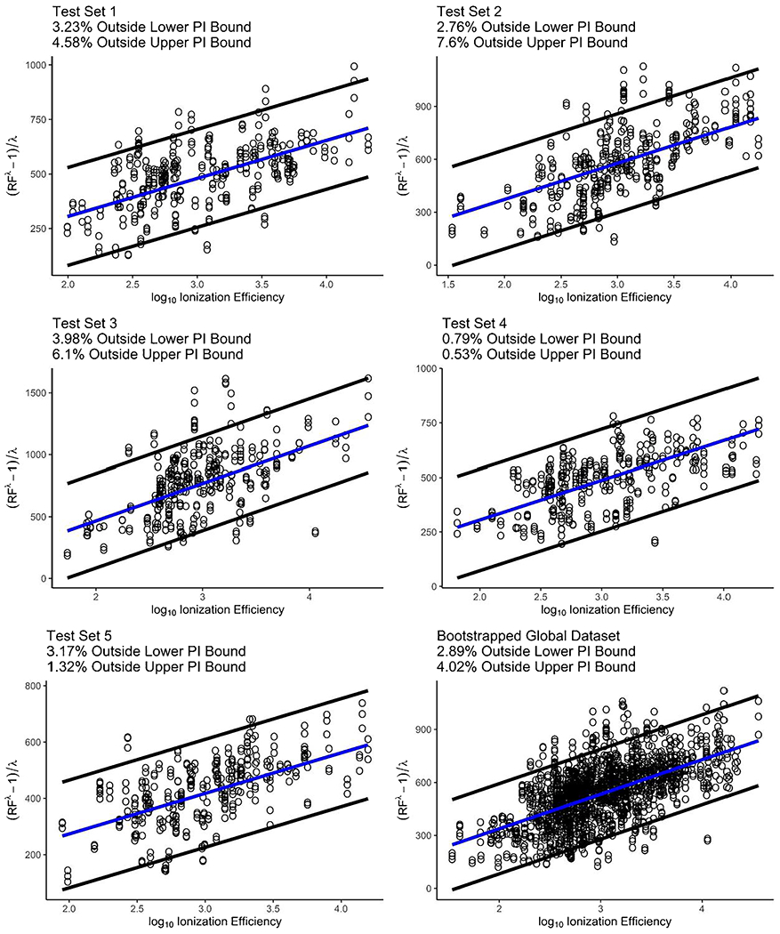
Linear mixed-effects model regressions of Box–Cox-transformed response factors (RF) on log-transformed predicted ionization efficiencies for ENTACT chemicals measures in ESI+ mode. The blue line represents the least-squares regression line from the mean bootstrap coefficients, and the region within the black lines represents the approximate 95% prediction interval about the regression line. Each figure panel shows the annotated percentage of data outside of the prediction interval bounds for a specific CV fold. The final plot shows the regression line and approximate 95% prediction interval for the full ESI+ dataset (Box–Cox lambda = 0.285)

Mixed-effects modeling results for ESI− mode data are shown in Figure S11. Across all five CV models, 0% to 3.94% of test set RF values were found below the estimated lower bounds, and 0% to 5.52% were found above the estimated upper bounds. Averaging across all five CV folds, the estimated 95% prediction intervals excluded 1.74% of RF values below ${\widehat{RF}}_{{0.025}_{IE}}$ and 0.14% of values above ${\widehat{RF}}_{{0.975}_{IE}}$. These results resemble those of the global bootstrap model, which excluded 1.45% (below ${\widehat{RF}}_{{0.025}_{IE}}$) and 1.59% (above ${\widehat{RF}}_{{0.975}_{IE}}$) of the global RF data.

Quantitative prediction error across methods

ESI+ mode

A total of 1,940 Y_obs values were available from 530 unique compounds in the ESI+ dataset. All 1,940 values yielded ${\widehat{Conc}}_{CC}$, ${\widehat{Conc}}_{{0.975}_{RF}}$, and ${\widehat{Conc}}_{{0.975}_{IE}}$ predictions, and 591 yielded ${\widehat{Conc}}_{{0.975}_{CC}}$ predictions (given finite inverse prediction intervals for chemical-specific calibration curves). All chemical- and method-specific concentration estimates are provided in Table S1. Cumulative percentile plots of error quotients are further provided in Fig. 4, with supporting violin plots given in Figure S12.

Fig. 4.

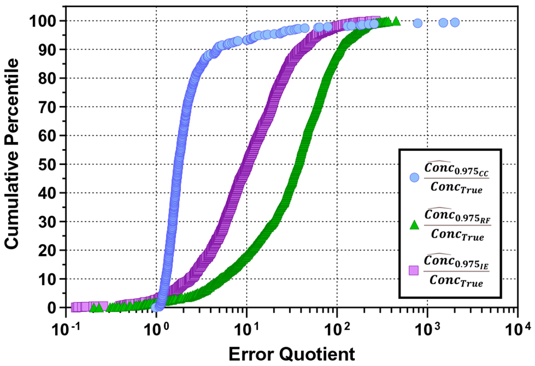
Cumulative percentile plot for error quotients based on three concentration estimation methods. ${\widehat{Conc}}_{{0.975}_{CC}}$ represents the upper-bound concentration prediction using chemical-specific calibration curves. ${\widehat{Conc}}_{{0.975}_{RF}}$ represents the upper-bound concentration prediction using the bounded response factor method. ${\widehat{Conc}}_{{0.975}_{IE}}$ represents the upper-bound concentration prediction using the ionization efficiency estimation method. Conc_True represents the true (known) analyte concentration. Three extreme outlier error quotients are not pictured $({\widehat{Conc}}_{{0.975}_{CC}}/Con{c}_{True}=1.62\times {10}^8,2.30\times {10}^8,\text{and}4.25\times {10}^{20})$, resulting from inverse predictions on three of the six data points for 1,3-diphenylguanidine

Half of the ${\widehat{Conc}}_{{0.975}_{CC}}$ values were within a factor of 1.8 of Conc_True, 93% were within a factor of 10 of Conc_True, and 98% were within a factor of 100 of Conc_True. Visual inspection of chemical-specific calibration curves showed that elevated error quotients were a product of high variance in Y_obs at a fixed concentration. Variable intensity measures contributed to wide 95% prediction intervals and elevated upper-bound concentration confidence limits (Figure S13). The magnitude of this prediction inaccuracy likely reflects uncontrolled error associated with semi-automated NTA sample analysis and data processing procedures.

For the bounded response factor method, 94.8% of Conc_True values were contained within the estimated 95% confidence interval (Table S1). Regarding the accuracy of the upper-bound estimates, 18% of ${\widehat{Conc}}_{{0.975}_{RF}}$ values were within a factor of 10 of Conc_True, 88% were within a factor of 100 of ${\widehat{Conc}}_{{0.975}_{RF}}$, and all ${\widehat{Conc}}_{{0.975}_{RF}}$ values were within a factor of 451 of Conc_True (Figs. 4 and S12). The lower left tail of the cumulative percentile plot shows that 1.7% of error quotients associated with ${\widehat{Conc}}_{{0.975}_{RF}}$ were less than 1, owing to a small percentage of RF values being below ${\widehat{RF}}_{0.025}$ (Table 1). In the most extreme of these cases, ${\widehat{Conc}}_{{0.975}_{RF}}$ underestimated Conc_True by a factor of 4.9 (Table S1).

For the ionization efficiency estimation method, 93% of Conc_True values were contained within the estimated 95% confidence interval (Table S1). Sixty imputations of $R{F}_{min}/\sqrt{2}$ (along with 1,880 unique ${\widehat{RF}}_{{0.025}_{IE}}$) were ultimately used to generate upper-bound concentration estimates (Figure S14). Forty-nine and 98% of the ${\widehat{Conc}}_{{0.975}_{IE}}$ values were within a factor of 10 and 100 of Conc_True, respectively, and all ${\widehat{Conc}}_{{0.975}_{IE}}$ values were within a factor of 267 of Conc_True. Considering the lower left tail of the cumulative percentile plot (Fig. 4), 2.8% of error quotients associated with ${\widehat{Conc}}_{{0.975}_{IE}}$ were less than 1, reflecting individual RF values below ${\widehat{RF}}_{{0.025}_{IE}}$. The most extreme underestimation of Conc_True using ${\widehat{Conc}}_{{0.975}_{IE}}$ was by a factor of 14.

Out of 1,617 observations where ${\widehat{Conc}}_{{0.975}_{RF}}>{\widehat{Conc}}_{{0.975}_{IE}}$, prediction quotients (i.e., ${\widehat{Conc}}_{{0.975}_{RF}}/{\widehat{Conc}}_{{0.975}_{IE}}$) were ≤ 10 for ~80% of the compounds and between 10 and 50 for the remaining compounds (Table S1). These results indicate considerable reductions in prediction error for many ENTACT chemicals when using ${\widehat{Conc}}_{{0.975}_{IE}}$ instead of ${\widehat{Conc}}_{{0.975}_{RF}}$. Importantly, the reduction in prediction error was realized only for chemicals with predicted log₁₀(IE) values exceeding a threshold of log₁₀(IE) = 2.567. Above this value of log₁₀(IE), the lower 95% prediction bound from the linear mixed-effects model yielded RF estimates greater than ${\widehat{RF}}_{0.025}$ from the global RF distribution.

ESI–mode

A total of 691 Y_obs values were available from 273 unique compounds in the ESI–dataset. All 691 values yielded ${\widehat{Conc}}_{CC}$, ${\widehat{Conc}}_{{0.975}_{RF}}$, and ${\widehat{Conc}}_{{0.975}_{IE}}$ predictions, and 80 yielded ${\widehat{Conc}}_{{0.975}_{CC}}$ predictions. All chemical- and method-specific results are provided in Table S2. Distributions of error quotients based on all three concentration estimation methods are further shown in Figures S15 and S16.

Half of the ${\widehat{Conc}}_{{0.975}_{CC}}$ values were within a factor of 2 of Conc_True, 95% were within a factor of 10 of Conc_True, and all were within a factor of ~50 of Conc_True. For the bounded response factor method, 94.9% of Conc_True values were contained within the estimated 95% confidence interval (Table S2). Regarding the accuracy of the upper-bound estimates, 50% of ${\widehat{Conc}}_{{0.975}_{RF}}$ values were within a factor of 10 of Conc_True, 92% were within a factor of 100 of Conc_True, and all ${\widehat{Conc}}_{{0.975}_{RF}}$ values were within a factor of ~335 of Conc_True. The lower left tail of the cumulative percentile plot (Figure S15) shows that 1.7% of error quotients associated with ${\widehat{Conc}}_{{0.975}_{RF}}$ were less than 1, owing to individual RF values being below ${\widehat{RF}}_{0.025}$. In the most extreme of these cases, ${\widehat{Conc}}_{{0.975}_{RF}}$ underestimated Conc_True by a factor of 3.3 (Table S2).

For the ionization efficiency estimation method, 97% of Conc_True values were contained within the estimated 95% confidence interval (Table S2). No imputations of $R{F}_{min}/\sqrt{2}$ were needed to generate upper-bound concentration estimates (Figure S14). Forty-nine and 93% of ${\widehat{Conc}}_{{0.975}_{IE}}$ values were within a factor of 10 and 100 of Conc_True, respectively, and all ${\widehat{Conc}}_{{0.975}_{IE}}$ values were within a factor of ~250 of Conc_True. Considering the lower left tail of the cumulative percentile plot (Figure S15), 1.3% of error quotients associated with ${\widehat{Conc}}_{{0.975}_{IE}}$ were less than 1, reflecting individual RF values below ${\widehat{RF}}_{{0.025}_{IE}}$. The most extreme underestimation of Conc_True using ${\widehat{Conc}}_{{0.975}_{IE}}$ was by a factor of 3.1.

Out of 355 observations (51%) where ${\widehat{Conc}}_{{0.975}_{RF}}>{\widehat{Conc}}_{{0.975}_{IE}}$, prediction quotients (i.e., ${\widehat{Conc}}_{{0.975}_{RF}}/{\widehat{Conc}}_{{0.975}_{IE}}$) were always less than 2 (Table S2). These results indicate only minor reductions in prediction error when using ${\widehat{Conc}}_{{0.975}_{IE}}$ instead of ${\widehat{Conc}}_{{0.975}_{RF}}$. Importantly, the reduction in prediction error was realized for chemicals with predicted log₁₀(IE) values exceeding a threshold of log₁₀(IE) = 1.326. Above this value of log₁₀(IE), the lower 95% prediction bound from the linear mixed-effects model yielded RF estimates greater than ${\widehat{RF}}_{0.025}$ from the global RF distribution.

Discussion

Non-targeted analysis using HRMS has quickly become a “go-to” analytical tool for identifying previously unknown or understudied organic chemical stressors in virtually any sample matrix. Most NTA applications, to date, have focused on compound identification with little consideration for compound quantitation. Yet, stakeholder needs are beginning to shift research foci beyond chemical identification and towards rapid risk-based evaluation [34, 35]. Such a shift requires tenable solutions — those with which compound quantification is not only possible, but achievable with computational efficiency, instrument transferability, and demonstrable statistical rigor. With tenable solutions in hand, emphasis can be placed on identifying emerging stressors that are most likely to pose unacceptable risks and on recommending rigorous targeted analyses for select high-priority analytes.

Previous qNTA studies have employed numerous approaches to generate point estimates of concentrations for individual analytes. Been et al. [34] quantified 92 analytes of interest in river water samples using model-predicted RFs. Results showed a mean prediction error of 5× and a maximum error of 29×, depending on chromatographic parameters. Kruve et al. [36] quantified 341 groundwater analytes using surrogate and model-predicted RF values. These methods yielded mean errors ranging from 1.8× to 3.8× and maximum errors ranging from 7× to 88×. Liigand and colleagues [23] quantified 35 mycotoxins and pesticides in cereals, with a mean prediction error of 5.4× and a maximum error of 62×. Finally, Abrahamsson et al. [37] used random forest and artificial neural network models to examine hundreds of analytes from ENTACT (a very similar dataset to that used here) as well as 57 polar endogenous compounds. Results showed model-based errors ranging up to ~6× (approximated using data provided in article supporting information).

Performance comparison across published studies is extremely challenging given variations in sampled matrices, laboratory procedures, mathematical techniques, and reported accuracy metrics. Yet, one commonality across most studies is the reporting of point concentration estimates for detected analytes. It must be realized that point predictions can over- or underestimate true values, generally with limited indication as to the direction and magnitude of error. Moving forward, if qNTA estimates are to be considered in risk-based evaluations, it will be important to provide confidence limits with each prediction. Then, out of an abundance of caution, upper-bound estimates can be compared to hazard/toxicity/bioactivity levels to support provisional risk-based evaluation. This margin-of-safety approach was recently outlined by McCord et al. [38] and serves as the framework for the current investigation. Given this focus, all interpretations of prediction error in the current article are based on upper-bound concentration estimates. Method success is then primarily defined by the frequency with which bounded estimates encapsulate the true value and secondarily by the magnitude of prediction error.

The bounded response factor method described here is a naive qNTA method, to be used for cursory analyte evaluation in the absence of confident structural information and/or IE predictions. This method is expected to yield the widest confidence intervals for each analyte (compared to other qNTA methods), with the interval width a function of the empirical RF distribution. Here, we observed the central 95% of RF values within a 177-fold range for ESI+ data and a 163-fold range for ESI− data. Given Y_obs for any analyte, we would calculate (using Eq. 1a and 1b) the same numerical span between ${\widehat{Conc}}_{{0.975}_{RF}}$ and ${\widehat{Conc}}_{{0.025}_{RF}}$. In other words, knowing nothing about the structure of the identified analyte, we would bound the estimated concentration (with 95% confidence) within a ~170-fold range given a single observed intensity. Results of the bounded response factor method showed −98% of ${\widehat{Conc}}_{{0.975}_{RF}}$ values greater than the true concentration, with median error of 37× (ESI+) and 10×(ESI−) and maximum error of 451× (ESI+) and 336× (ESI−). Results further showed ~2% of ${\widehat{Conc}}_{{0.975}_{RF}}$ values less than the true concentration, with the magnitude of error never exceeding ~5×. These findings highlight the statistical suitability of the default qNTA method, with an expected (approximate) percentage of ${\widehat{Conc}}_{{0.975}_{RF}}$ values underestimating the true value. They further highlight an opportunity to considerably reduce the magnitude of overestimation for certain analytes by incorporating molecular descriptors to bound RF predictions.

The ionization efficiency estimation method was used to reduce estimation error while preserving statistical confidence. Given predicted IE for each ENTACT chemical, ~98% of ${\widehat{Conc}}_{{0.975}_{IE}}$ values were again greater than the true concentration, but with median error of ~10× (for both ESI+ and ESI−) and maximum error of 267× (ESI+) and 249× (ESI−). These results indicate considerable improvement over the naïve bounded response factor results for ESI+ data. As enhanced IE prediction methods are developed for all manner of NTA data (e.g., ESI+, ESI−, APCI+, APCI−), they can easily be calibrated to empirical RF values to aid quantitative estimation, as shown here. It must be noted, however, that the ionization efficiency estimation method is considerably more rigid than the non-parametric bounded response factor method. First, it requires mathematical transformation of empirical RF values to ensure linearity and homoscedasticity; each new data set may require alternative transformation approaches to meet regression assumptions. Second, it requires a mixed-effects modeling approach to account for correlation between replicates of the same analyte. Finally, it requires multi-step bootstrapping procedures to estimate a prediction interval about the linear regression line. In light of these challenges, future applications should consider alternative parametric or non-parametric procedures that allow for non-linearities and repeat measures and that readily produce confidence or credible intervals. Such an approach would allow maximum flexibility for virtually any NTA dataset.

NTA generally makes use of partially automated work-flows, where the number of features can be too numerous for exhaustive manual review. As an important benchmarking process for this qNTA study, we estimated the amount of quantitative error stemming from semi-automated processing procedures. Specifically, we developed chemical-specific calibration curves for a subset of ENTACT analytes that were measured at multiple concentrations in multiple mixtures. The intensity values (Y term) for these calibration curves were automatically generated using NTA software [22]. Prediction interval width therefore reflects the extent of intensity measurement error at a given concentration for a given analyte. Considering upper-bound concentration estimates (via inverse prediction), we observed a median error of ~2× for both ESI+ and ESI− data and maximum error of 54× for ESI− data. Notwithstanding three extreme outliers for 1,3-diphenylguanidine (Figure S13), the maximum error for ESI+ data reached ~2000×, with ~99% of values < 200× (Figs. 4 and S12). These results clearly indicate some level of underlying “noise” for most analytes, and considerable measurement error for a small portion of measured analytes. Clearly these errors could be reduced using more sophisticated sample and batch correction techniques and/or matched internal standards. Researchers must carefully weigh the feasibility of these correction procedures in future NTA studies. As it stands, for this study, measurement error across replicate samples clearly contributed to the total prediction error associated with each qNTA method. We therefore strongly encourage future investigations to consider basic measurement error as a source of uncertainty in qNTA predictions.

The methods described here offer a straightforward means to statistically bound concentration estimates for identified chemicals given HRMS-measured intensities. These methods serve as a critical starting point for the risk-based evaluation of emerging environmental and biological contaminants. The utilized mathematical procedures were carefully developed and rigorously evaluated. Results of these procedures highlight areas in which future research and development may be needed to bolster performance for real-world qNTA applications. Specifically, the underlying RF data used for this study were heavily skewed and even exhibited a slightly non-normal character after optimal data transformation. During cross-validation, some extreme RF values at the distribution tails (Figures S9 and S10) led to variable estimates of RF prediction intervals, which in turn led to variable exceedance percentages (Tables 1 and 2; Figs. 3 and S11). Indeed, using the bounded response factor method, exceedance percentages ranged from 0 to 7.83%, and using the ionization efficiency estimation method, they ranged from 0 to 7.6%. Since an exceedance of 2.5% is expected in each case, these results highlight a need to further explore the generalizability of these uncertainty estimation methods. Such exploration should be performed using larger and more variable datasets, with a goal of capturing the full amenability space of any selected analytical method.

The ENTACT mixtures examined here proved a suitable compilation of organic analytes with which to develop and test initial qNTA methods. Moving forward, a need exists for optimized calibrant mixtures to suit a variety of analytical methods. The NTA research community should carefully coordinate the design, preparation, and dissemination of these mixtures to aid those wishing to implement qNTA procedures. The community should further coordinate the development of optimized/consensus IE prediction methods to suit numerous NTA methods and attempt to standardize performance metrics to be reported in qNTA studies. Finally, in future works, consideration must be given to factors that affect analyte quantitation across a wealth of diverse sample matrices. The methods described herein focused entirely on compound quantitation in a prepared solvent (akin to a sample extract). Dedicated efforts must now focus on the effects of analyte recovery on final compound quantitation in the original sampled matrix [38]. This is indeed a daunting challenge given the vast array of matrix types, extraction conditions, and potential organic analytes of interest. Despite this challenge, a clear path now exists towards the implementation of robust qNTA methods for myriad applications. This article marks a major step towards utilizing qNTA estimates to support provisional risk-based decisions on emerging chemical stressors.

References

- 1.Egeghy PP, Judson R, Gangwal S, Mosher S, Smith D, Vail J, et al. The exposure data landscape for manufactured chemicals. Sci Total Environ. 2012:414:159–66. [DOI] [PubMed] [Google Scholar]
- 2.Weinberg N, Nelson D, Sellers K, Byrd J. Insights from TSCA reform: a case for identifying new emerging contaminants. Curr Pollut Rep. 2019;5(4):215–27. [Google Scholar]
- 3.Risk assessment in the federal government: managing the process. National Research Council (US). Washington (DC): National Academies Press (US); 1983. [PubMed] [Google Scholar]
- 4.Newton SR, McMahen RL, Sobus JR, Mansouri K, Williams AJ, McEachran AD, et al. Suspect screening and non-targeted analysis of drinking water using point-of-use filters. Environ Pollut. 2018;234:297–306. [DOI] [PMC free article] [PubMed] [Google Scholar]
- 5.Postigo C, Andersson A, Harir M, Bastviken D, Gonsior M, Schmitt-Kopplin P, et al. Unraveling the chemodiversity of halogenated disinfection by-products formed during drinking water treatment using target and non-target screening tools. J Hazard Mater. 2021;401. [DOI] [PubMed] [Google Scholar]
- 6.Sapozhnikova Y Non-targeted screening of chemicals migrating from paper-based food packaging by GC-Orbitrap mass spectrometry. Talanta. 2021;226. [DOI] [PubMed] [Google Scholar]
- 7.Christia C, Poma G, Caballero-Casero N, Covaci A. Suspect screening analysis in house dust from Belgium using high resolution mass spectrometry; prioritization list and newly identified chemicals. Chemosphere. 2021;263. [DOI] [PubMed] [Google Scholar]
- 8.Moschet C, Anumol T, Lew BM, Bennett DH, Young TM. Household dust as a repository of chemical accumulation: new insights from a comprehensive high-resolution mass spectrometric study. Environ Sci Technol. 2018;52(5):2878–87. [DOI] [PMC free article] [PubMed] [Google Scholar]
- 9.Newton SR, Sobus JR, Ulrich EM, Singh RR, Chao A, McCord J, et al. Examining NTA performance and potential using fortified and reference house dust as part of EPA’s Non-Targeted Analysis Collaborative Trial (ENTACT). Anal Bioanal Chem. 2020;412(18):4221–33. [DOI] [PMC free article] [PubMed] [Google Scholar]
- 10.Gravert TKO, Vuaille J, Magid J, Hansen M. Non-target analysis of organic waste amended agricultural soils: characterization of added organic pollution. Chemosphere. 2021;280. [DOI] [PubMed] [Google Scholar]
- 11.Chiaia-Hernandez AC, Gunthardt BF, Frey MP, Hollender J. Unravelling contaminants in the Anthropocene using statistical analysis of liquid chromatography-high-resolution mass spectrometry nontarget screening data recorded in lake sediments. Environ Sci Technol. 2017;51(21):12547–56. [DOI] [PubMed] [Google Scholar]
- 12.Shah NH, Noe MR, Agnew-Heard KA, Pithawalla YB, Gardner WP, Chakraborty S, et al. Non-targeted analysis using gas chromatography-mass spectrometry for evaluation of chemical composition of E-vapor products. Front Chem. 2021;9. [DOI] [PMC free article] [PubMed] [Google Scholar]
- 13.Lowe CN, Phillips KA, Favela KA, Yau AY, Wambaugh JF, Sobus JR, et al. Chemical characterization of recycled consumer products using suspect screening analysis. Environ Sci Technol. 2021;55(16):11375–87. [DOI] [PMC free article] [PubMed] [Google Scholar]
- 14.Abrahamsson DP, Wang AL, Jiang T, Wang MM, Siddharth A, Morello-Frosch R, et al. A comprehensive non-targeted analysis study of the prenatal exposome. Environ Sci Technol. 2021;55(15):10542–57. [DOI] [PMC free article] [PubMed] [Google Scholar]
- 15.Plassmann MM, Fischer S, Benskin JP. Nontarget time trend screening in human blood. Environ Sci Tech Let. 2018;5(6):335–40. [Google Scholar]
- 16.Teehan P, Schall MK, Blazer VS, Dorman EL. Targeted and non-targeted analysis of young-of-year smallmouth bass using comprehensive two-dimensional gas chromatography coupled with time-of-flight mass spectrometry. Sci Total Environ. 2021;806(2). [DOI] [PubMed] [Google Scholar]
- 17.Tian ZY, Zhao HQ, Peter KT, Gonzalez M, Wetzel J, Wu C, et al. A ubiquitous tire rubber-derived chemical induces acute mortality in coho salmon. Science. 2021;371(6525):185–9. [DOI] [PubMed] [Google Scholar]
- 18.Place BJ, Ulrich EM, Challis JK, Chao A, Du B, Favela KA, et al. An introduction to the benchmarking and publications for non-targeted analysis working group. Anal Chem. 2021;93(49):16289–96. [DOI] [PMC free article] [PubMed] [Google Scholar]
- 19.Peter KT, Phillips AL, Knolhoff AM, Gardinali PR, Manzano CA, Miller KE, et al. Nontargeted analysis study reporting tool: a framework to improve research transparency and reproducibility. Anal Chem. 2021;93(41):13870–9. [DOI] [PMC free article] [PubMed] [Google Scholar]
- 20.Schymanski EL, Jeon J, Gulde R, Fenner K, Ruff M, Singer HP, et al. Identifying small molecules via high resolution mass spectrometry: communicating confidence. Environ Sci Technol. 2014;48(4):2097–8. [DOI] [PubMed] [Google Scholar]
- 21.Nunez JR, Colby SM, Thomas DG, Tfaily MM, Tolic N, Ulrich EM, et al. Evaluation of in silico multifeature libraries for providing evidence for the presence of small molecules in synthetic blinded samples. J Chem Inf Model. 2019;59(9):4052–60. [DOI] [PMC free article] [PubMed] [Google Scholar]
- 22.Sobus JR, Grossman JN, Chao A, Singh R, Williams AJ, Grulke CM, et al. Using prepared mixtures of ToxCast chemicals to evaluate non-targeted analysis (NTA) method performance. Anal Bioanal Chem. 2019;411(4):835–51. [DOI] [PMC free article] [PubMed] [Google Scholar]
- 23.Liigand J, Wang TT, Kellogg J, Smedsgaard J, Cech N, Kruve A. Quantification for non-targeted LC/MS screening without standard substances. Sci Rep. 2020;10(1). [DOI] [PMC free article] [PubMed] [Google Scholar]
- 24.Malm L, Palm E, Souihi A, Plassmann M, Liigand J, Kruve A. Guide to semi-quantitative non-targeted screening using LC/ESI/HRMS. Molecules. 2021;26(12). [DOI] [PMC free article] [PubMed] [Google Scholar]
- 25.Kruve A Strategies for drawing quantitative conclusions from nontargeted liquid chromatography-high-resolution mass spectrometry analysis. Anal Chem. 2020;92(7):4691–9. [DOI] [PubMed] [Google Scholar]
- 26.Go YM, Walker DI, Liang YL, Uppal K, Soltow QA, Tran V, et al. Reference standardization for mass spectrometry and high-resolution metabolomics applications to exposome research. Toxicol Sci. 2015; 148(2):531–43. [DOI] [PMC free article] [PubMed] [Google Scholar]
- 27.Aalizadeh R, Panara A, Thomaidis NS. Development and application of a novel semi-quantification approach in LC-QToF-MS analysis of natural products. J Am Soc Mass Spectr. 2021;32(6):1412–23. [DOI] [PubMed] [Google Scholar]
- 28.Ulrich EM, Sobus JR, Grulke CM, Richard AM, Newton SR, Strynar MJ, et al. EPA’s non-targeted analysis collaborative trial (ENTACT): genesis, design, and initial findings. Anal Bioanal Chem. 2019;411(4):853–66. [DOI] [PMC free article] [PubMed] [Google Scholar]
- 29.Fox J, Weisberg S. An R companion to applied regression. 3rd ed. Thousand Oaks, California, USA: Sage; 2019. [Google Scholar]
- 30.Greenwell BM, Kabban CMS. investr: an R package for inverse estimation. R J. 2014;6(1):90–100. [Google Scholar]
- 31.R Core Team. R: a language and environment for statistical computing. Vienna: Austria; 2020. [Google Scholar]
- 32.Peterson RA. Finding optimal normalizing transformations via bestNormalize. R J. 2021;13(1):310–29. [Google Scholar]
- 33.Bates D, Mächler M, Bolker B, Walker S. Fitting linear mixed-effects models using lme4. J Stat Softw. 2015;67(1):1–48. [Google Scholar]
- 34.Been F, Kruve A, Vughs D, Meekel N, Reus A, Zwartsen A, et al. Risk-based prioritization of suspects detected in riverine water using complementary chromatographic techniques. Water Res. 2021;204. [DOI] [PubMed] [Google Scholar]
- 35.Liu Q, Li L, Zhang X, Saini A, Li W, Hung H, et al. Uncovering global-scale risks from commercial chemicals in air. Nature. 2021;600:456–61. [DOI] [PubMed] [Google Scholar]
- 36.Kruve A, Kiefer K, Hollender J. Benchmarking of the quantification approaches for the non-targeted screening of micropollutants and their transformation products in groundwater. Anal Bioanal Chem. 2021;413(6):1549–59. [DOI] [PMC free article] [PubMed] [Google Scholar]
- 37.Abrahamsson DP, Park JS, Singh RR, Sirota M, Woodruff TJ. Applications of machine learning to in silico quantification of chemicals without analytical standards. J Chem Inf Model. 2020;60(6):2718–27. [DOI] [PMC free article] [PubMed] [Google Scholar]
- 38.McCord JP, Groff LC, Sobus JR. Quantitative non-targeted analysis: bridging the gap between contaminant discovery and risk characterization. Environ Int. 2022;158. [DOI] [PMC free article] [PubMed] [Google Scholar]
Associated Data
This section collects any data citations, data availability statements, or supplementary materials included in this article.