

SUMMARY
Flexibility is a hallmark of memories that depend on the hippocampus. For navigating animals, flexibility is necessitated by environmental changes such as blocked paths and extinguished food sources. To better understand the neural basis of this flexibility, we recorded hippocampal replays in a spatial memory task where barriers as well as goals were moved between sessions to see whether replays could adapt to new spatial and reward contingencies. Strikingly, replays consistently depicted new goal-directed trajectories around each new barrier configuration and largely avoided barrier violations. Barrier-respecting replays were learned rapidly and did not rely on place cell remapping. These data distinguish sharply between place field responses, which were largely stable and remained tied to sensory cues, and replays, which changed flexibly to reflect the learned contingencies in the environment and suggest sequenced activations such as replay to be an important link between the hippocampus and flexible memory.
In brief
Widloski and Foster show that place cells in rat hippocampus learn replay sequences around barriers, even after a large (>90) number of barrier reconfigurations. By contrast, cells’ place fields are largely stable, dissociating the stable representation of space from a powerful mechanism for the acquisition and recall of flexible memory.
INTRODUCTION
Flexibility in the use of learned associations about the world is critical to survival and has long been considered an indicator of cognition (Kohler, 1925; Tolman, 1948; Bayne et al., 2019). An important aspect of flexibility is the ability to adapt when the structure of the environment changes unexpectedly (Rashotte, 1987; Kabadayi et al., 2018; Hebb and Williams, 1946; Alvernhe et al., 2012; de Cothi et al., 2020). Dynamic environments pose a substantial challenge to animal navigation, requiring both flexibility within and rapid adaptation across contexts. Lesion studies point to the hippocampus as being essential for both aspects of behavioral flexibility. Hippocampal lesions in rodents produce deficits in the ability to flexibly navigate to a learned goal from unpredictable locations (Morris et al., 1982) or to make flexible inferences across learned odor pairs (Eichenbaum, 2004) and in humans leads to deficits in the ability to imagine new experiences (Hassabis et al., 2007). Moreover, damage to the hippocampus results in performance deficits on spatial replanning tasks that require the construction of novel routes to familiar goals in the presence of barriers or shortcuts (Thompson et al., 1984; Winocur et al., 2010; Maguire et al., 2006; Rosenbaum et al., 2015).
Hippocampal place cells fire selectively to the conjunction of spatial and nonspatial cues in the environment. As such, the hippocampus has been thought to encode a cognitive map of the environment (O’Keefe and Nadel, 1978), one that individuates states as well as encodes state relationships to support flexible, inferential behavior (Muller et al., 1996; Eichenbaum and Cohen, 2014; Whittington et al., 2020). The hippocampus readily forms distinct representations across contexts (Alme et al., 2014; Leutgeb et al., 2005; Wood et al., 2000; Frank et al., 2000; Ferbinteanu and Shapiro, 2003; Kennedy and Shapiro, 2009; Kentros et al., 2004; Muzzio et al., 2009; Monaco et al., 2014; Kelemen and Fenton, 2010; Muller and Kubie, 1987; Bostock et al., 1991; Moita et al., 2003; Komorowski et al., 2009), thus in theory enabling the formation of new cognitive maps adapted to the context-specific needs of the animal (Smith and Mizumori, 2006; Stachenfeld et al., 2017). However, remapping to encode context is not always observed (Berke et al., 2009; Ainge et al., 2012; Griffin and Hallock, 2013; Duvelle et al., 2019). Strikingly, place fields are largely unperturbed by the introduction and manipulation of barriers, whether or not those manipulations necessitate small (Muller and Kubie, 1987; Rivard et al., 2004) or large (Alvernhe et al., 2008, 2011; Duvelle et al., 2021) changes to the behavioral policy. This is especially perplexing given the importance of the hippocampus in such replanning tasks (Thompson et al., 1984; Winocur et al., 2010; Maguire et al., 2006; Rosenbaum et al., 2015), and raises the question of whether a significant but possibly more covert hippocampal neural correlate of behavioral adaptation to changes in spatial contingencies can be found.
Place cells participate in rapid sequenced reactivations called “awake replays” that can depict past and future behavior (Diba and Buzsá ki, 2007; Foster and Wilson, 2006; Davidson et al., 2009; Pfeiffer and Foster, 2013) and have been linked to planning (Jadhav et al., 2012; Pfeiffer and Foster, 2013) and memory consolidation (Dupret et al., 2010; Ego-Stengel and Wilson, 2010; Girardeau et al., 2009). Replay is increasingly seen as a generative process that reflects the behavioral contingencies of the environment rather than the specific experiences of the animal (Gupta et al., 2010; Foster, 2017) and is thus well suited to subserve behavioral flexibility. In addition, replay offers a unique window on hippocampal contextual coding without the confounding effects of behavior. However, nothing is known about how replays adapt to spatial contingency changes, especially when those changes are expected to elicit minimal changes to the hippocampal place code. We tested this by recording place cells and replay in a goal-directed task subject to repeated barrier manipulations that would dramatically and unpredictably alter the navigational requirements of the animal while minimally affecting the sensory perception of the environment (through the use of transparent barriers in a highly familiar environment). We used wireless ultra-high-density hyperdrives to record from hundreds of place cells simultaneously and across sessions, enabling us to measure replay during the learning of the task as well as ascertain changes in place fields across barrier configurations. This approach of tracking both place fields and replay allowed us to assess hippocampal adaptation to changing spatial contingencies at multiple resolutions to determine how place encoding and replay-based path encoding contribute to flexible learning.
RESULTS
Behavior is goal directed
Rats were trained on a spatial memory task in a square arena to search for liquid chocolate available in one of nine food wells, which alternated on consecutive trials between a learnable fixed location (Home well) and unpredictable other locations (Random wells), designated as Home and Random trials, respectively. In each trial, a variable time delay (5–15 s) passed before: (a) reward was provided at the bait location, and (b) for all Random trials, a light came on next to the rewarded well, cueing the approach. Before each session, transparent “jail-bar” barriers (Ólafsdóttir et al., 2015), permeable to visual and olfactory information, were placed in 6 out of 12 possible locations, in a novel, random selection from 924 possible configurations (Figures 1A and 1B). Two to three consecutive behavioral sessions were performed per day for a total of up to 94 sessions per rat with sessions separated by ~3–4 h, each with a novel barrier configuration (or in some cases, no barriers) as well as a novel, pseudo-randomly chosen Home location (Figure S1A) (47 sessions total; 12 sessions for rat 1, 17 sessions for rat 2, 8 sessions for rat 3, and 10 sessions for rat 4). Rats exhibited trial-selective spatial memory, as evidenced by greater Home-well visit probability during the unrewarded delay (Figures 1C and 1D) and greater anticipatory-licking duration at the Home well for Home versus Random trials (Figure 1E; Figure S1B).
Figure 1. Behavior is goal directed.

A) Photo of the maze interior showing transparent barriers, reward wells, and painted wall cues.
(B) Top: Behavioral trajectory (gray) from session 77, rat 1. Bottom: Barrier configurations for sessions 1 through 4.
(C) Behavioral trajectories across several trials from session 78, color-coded according to time within the trial. Trial phase and number are at bottom right. The rewarded well for each trial is outlined in red.
(D) Probability of the rat visiting the Home well (H) versus a Random well (R) within the first 5 s of the Home trial, as a function of trial number (left) or averaged across trials (right). Horizontal black line: p < 0.05. Hshuff is calculated the same as H except that the Home well ID was selected randomly. Colored lines indicate means for individual rats.
(E) Duration of anticipatory licking at the Home well for Home (H) versus Random (R) trials as a function of trial number (left) or averaged across trials (right). Horizontal black line, p < 0.05.
(D and E) n = 47 sessions (total number of recorded sessions from all rats); Wilcoxon sign-rank tests, ***p < 0.001; error bars are SEM.
Replay is goal directed and predictive of future behavior
In order to measure replay, we implanted four trained rats with headstages holding 64 independently-adjustable tetrodes (Figure S1C), which were lowered over the course of 2–4 weeks into the pyramidal cell layer of the CA1 subregion of dorsal hippocampus in both hemispheres. The headstages digitized and stored neural signals, enabling wireless recording during behavior, because wires would have constrained the rats’ behavior around the barriers. We recorded the activity of up to 295 hippocampal place cells simultaneously (Figure S1D) (mean per session = 156 cells; Rats 1–3 had >100 cells in every session and were included in replay analyses; Rat 4 had <100 cells in every session and was used for place field analysis only). In order to better understand the effect of barriers on replay, we recorded the same cells across multiple barrier configurations. Place fields were determined for each active cell, and memory-less Bayesian position estimation was used to decode the posterior probability of position from the spiking of all simultaneously recorded cells. During stopping periods in the task, candidate events were identified as continuous epochs lasting at least 100 ms where the decoded position changed smoothly (Figures S2A–S2G). Those candidate events that satisfied spatial coverage criteria were classified as replays (number of candidate events per session across 37 sessions: 2,652 ± 224; percentage of candidate events that were classified as replays: 5.7% ± 0.4%). As in previous studies with large-scale recordings, the posterior probability from each time bin during replay was so sharply defined that we could sum across time bins to produce a clear representation of the depicted two-dimensional trajectory through the environment (Figures 2A–2G; Figure S3). Replays initiated at Random wells when the rat was consuming chocolate there (Away-event replays) were more likely to terminate at the Home well than at other wells (Figure 2G; Figure S2H). Moreover, the probability of the rat visiting the Home well was higher if preceded by a Home-well-terminating replay (Figure 2H; Figure S2I). Further, the angular displacement between the decoded position within each replay time step and the immediate future or past trajectory of the animal revealed closer alignment to the future trajectory than to the past (Figure 2I; Figures S2J–S2M and S3E). Thus, in the barrier maze, as previously in the open field, replays exhibited memory for the goal location and predicted the immediate future behavior of the animal.
Figure 2. Replay is goal directed and predictive of future behavior.

(A–F) Replay examples from different sessions from rat 1, targeting (A) the Home well, (B) Random wells, or (C) the upper right corner of the maze (a preferred grooming location), as well as (D) stopping at or (E) passing through a barrier. The colored blob in each panel is the posterior probability of replay, defined as the summed posterior across time bins of the replay (time bin duration of 80 ms). The posterior has been binarized (by discarding bins where the posterior is less than 0.01) and color-coded according to elapsed time within the replay. Solid black line: replay center-of-mass. Gray segments indicate excluded time bins (see STAR Methods). Time within session is shown at the upper left (min:s). Replay duration (s) at upper right. (F) shows a long-duration example replay from rat 2.
(G) Probability of Away-event replays terminating at Home (H) versus Random (R) wells. Hshuff is calculated the same as H except that the Home well ID was selected randomly. Colored lines indicate means for individual rats.
(H) The occurrence of an Away-event replay terminating at the Home well versus probability of the rat visiting the Home well within the first 5 s of the subsequent Home trial.
(I) Absolute angular displacement between replay and the rat’s future and past path.
(G–I) n = 37 sessions (total number of recorded sessions from rats 1–3); Wilcoxon sign-rank tests, ***p < 0.001; error bars are SEM.
Replay rapidly and repeatedly adapts to conform to the barriers
While individual replay examples moved around barriers (Figures 2A–2C; Figures S3A, S3B, and S3F), the full extent of barrier conformity was evident from all the replays recorded during each session (Figures 3A and 3B; Figure S4). This was particularly striking because large numbers of conflicting barrier configurations had been experienced in the same environment prior to each session (76 by the third session in Figure 3A). In order to quantify conformity, we first partitioned each replay into constituent instantaneous velocity vectors. Each constituent vector was then scored based on its proximity and alignment to the local barrier structure in the environment (Figure 3C; Figure S5A): constituent vectors were scored high for moving parallel to nearby barriers and scored low for moving perpendicular to them, with constituent vectors close to barriers counting more heavily than those further away (Figure S5B). We defined the session-averaged barrier conformity score as the mean of all scores across all constituent replay vectors within the session. We then compared this score to a control distribution of session-averaged barrier conformity scores obtained when computed against the other 923 possible barrier configurations (Figure 3D). To address sampling differences between configurations conservatively, we removed from consideration constituent vectors very close to the barriers (Figure 3C). For 87% of sessions (27 out of 31 sessions with barriers), the session-averaged barrier conformity score for the actual barrier configuration exceeded the 95th percentile of the control distribution (binomial test, p < 0.001) (Figure S5C). Further, barrier conformity arose rapidly within each session (Figure 3E; Figure S3F) and showed no dependence on rat heading (Figure S5D). In order to assess how far barrier conformity persisted from the barriers, we removed the proximity-to-barrier weighting (Figure S5B) and recalculated the scores as a function of distance to the nearest barrier. Barrier conformity was found to extend nearly 18 cm from the barriers (Figure 3F), nearly the minimum inter-well distance Together, these results show that replays adapted to conform to the barriers in each new configuration, that the adaptation was rapid, and that barrier conformity was spatially extended and unlikely to depend on visual guidance.
Figure 3. Replays rapidly adapt to conform to the barriers.
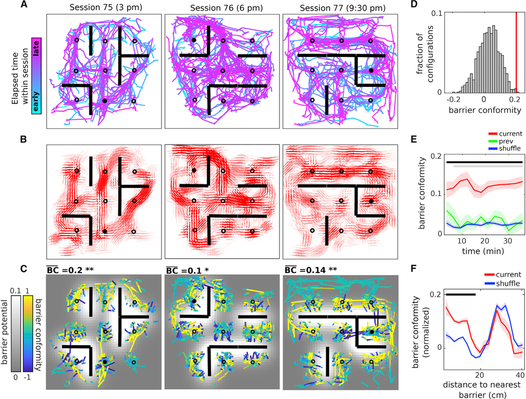
A) All replays from sessions 75, 76, and 77 recorded on the same day from rat 2, color-coded according to elapsed time within session.
(B) Local averaging of replay orientation as a function of position within the environment. For each bin, the mean vector orientation and length are plotted for the distribution of replay orientations (modulo 180) found within a circle of radius 2 bins. Color transparency indicates the number of data points (orientations) used to compute each mean vector.
(C) Replays from (A) have been decomposed into their constituent vectors (with 80 ms time bins) and color-coded according to barrier conformity score. Vectors starting near the 12 barrier positions have been removed. The background image is the barrier potential. The session-averaged barrier conformity score and significance are at the upper left of each panel.
(D) The session-averaged barrier conformity score for session 75 (red vertical line) and the distribution of scores with respect to all other possible barrier configurations (gray histogram, “shuffle”). The barrier conformity p value for the session is the fraction of scores greater than the red line.
(E) Barrier conformity as a function of time within the session, computed within a 6 min sliding window, with respect to the current (red), previous (green), and shuffled (blue) barrier configurations. Horizontal lines (p < 0.05), comparison of current barrier configuration scores with previous (gray) and shuffle (black) scores. Current condition: n = 31 sessions, which is the total number of recorded sessions with barriers from rats 1–3. Previous condition: n = 16, which is the total number of recorded sessions with barriers that had a corresponding previous session on the same day.
(F) Barrier conformity as a function of distance to the nearest barrier, with respect to the current (red) and shuffled (blue) barrier configurations. Horizontal blackline, p < 0.05. The large peak near 30 cm (approximately the mean wall-to-barrier distance) is the effect of local alignment to the walls. Wilcoxon sign-rank tests; error bars are SEM.
The barriers are impermeable to most activity during immobility periods
An alternative hypothesis for the observed barrier conformity was that our criterion for detecting replay was biased because of a lack of place field coverage near barriers, either because of behavioral sampling or altered place fields. Therefore, we developed a second measure of activity that did not require selection of replays but instead analyzed the spiking activity in all candidate events. Moreover, the measure assessed the relationship between the representation of pairs of locations irrespective of the representation of locations between them, where data might be missing. For each position, we calculated the posterior probability as a time series (Figure 4A, top). We then used the cross-correlogram between pairs of time series to define a “time lag” between the two associated positions (Figure 4A, bottom; Figure S6A): this represented the latency at which, on average, representation of the first position was followed by representation of the second. Finally, time lag maps were constructed from the time lags of one reference location to all other locations (Figure 4B; Figure S6B). We hypothesized that barrier conformity would be reflected in greater time lags between positions straddling a barrier than not. Moreover, such a finding would indicate a much more prevalent effect than for replay because candidate events accounted for ten times as many spikes as replay events during immobility periods (Figure 4C; Figure S6C). Indeed, examination of time lag maps for a set of different reference locations (Figure 4B, columns) across different barrier configurations (Figure 4B, rows) revealed a striking effect of the barriers, squashing low time lag regions (shown in dark blue) up against the barriers, and elongating them in unobstructed regions. To quantify this effect, slices of the maps extending from the reference location toward the nearest barrier were extracted (Figure 4D; Figure S6A). As expected, we found that the rise in time lags occurred sooner the closer the reference bin was to a barrier (Figure 4E, solid line). As a control, we repeated the analysis with respect to barriers located at the six complementary positions in the maze, in which case we found no such dependence (Figure 4D, inset; Figure 4E, dashed line). Lastly, we used multi-dimensional scaling (Gustafson and Daw, 2011; Buja et al., 2008) to translate temporal lags into spatial offsets, reducing the full set of time lag maps (L2 numbers, where L is the number of spatial bins per dimension) into a distorted lattice in the Euclidean plane (2L numbers) (Figure 4F; Figures S6D–S6F). Deformations around barriers were clearly visible, indicative of the relative inaccessibility of states on opposite sides of the barrier. Together, these results indicate that not just replay but most population activity during stopping periods exhibited learned avoidance of the current session’s configuration of barriers.
Figure 4. The barriers are impermeable to most activity during immobility periods.

(A) Schematic showing how time lags are computed. Top: Each frame is the decoded posterior probability across spatial bins within a 20 ms window. Two candidate sequences are shown. White frames indicate dataset to zero. Bottom: Example cross-correlogram (gray: raw curve; black: smoothed with Gaussian kernel, 60 ms SD) computed from the posterior probability time series from a pair of spatial bins (long horizontal red dashed lines in the top plot), with the vertical red line indicating the latency at the peak. The time lag is defined as the absolute value of this latency.
(B) Representative time lag maps taken from sessions 76, 77, and 78, rat 1. The red square is the map’s reference bin.
(C) The fraction of spikes during immobility is defined as the total number of spikes within all candidate sequences and replays divided by the total number of spikes within all immobility periods (rat speed < 5 cm/s) within the session (n = 37 sessions, which is the total number of recorded sessions from rats 1–3).
(D) Time lag map slices grouped according to the distance from the reference bin to the nearest barrier (cool-to-hot colors represent near-to-far distances) (n = 31 sessions, which is the total number of sessions with barriers from rats 1–3). Inset: Same as main figure, except slices are taken with respect to the barriers in the remaining six positions in the maze (“complementary barrier configuration”).
(E) Integrated areas under the slices for the data in (D) for the actual (solid line: Pearson’s r = −0.6, p < 0.001) and the complementary (dashed line: Pearson’s r = −0.11, n.s.) barrier configurations.
(F) Left: Multi-dimensional scaling applied to session 79 time lag maps. Right: The same grid prior to deformation. Wilcoxon sign-rank tests, **p < 0.01, ***p < 0.001; error bars are SEM.
The majority of place cells are stable across sessions
In order to gain a more mechanistic understanding of replay adaptation, we next sought to understand to what extent this adaptation was mirrored at the level of changes to the underlying hippocampal map. We tracked single units across multiple barrier configurations and compared the rate maps and population vectors (PVs) (the set of firing rates at a spatial bin across all active cells) across pairs of neighboring sessions (Figure 5A; Figures S7 and S8A–S8C). Surprisingly, we found that a majority of pairwise session correlation measurements across cells and across spatial locations were stable (rate maps: 1,686 of 2,887 comparisons [58%] were stable across 27 session pairs with an average of 107 cell comparisons per session pair; a binomial test indicated that the proportion of stable cell comparisons was higher than expected by chance [p < 0.001, two-sided, n = 2,887], assuming a chance level of stability for each cell was 0.5; mean fraction of stable cells per session: 0.58 ± 0.02, n = 27 session pairs; PVs: 28,788 of 33,245 comparisons [87%] were stable across 27 session pairs with an average of 1,231 bin comparisons per session pair, where bins are 2 cm per dimension; a binomial test using coarse-grained rate maps to compute the PV correlations [see STAR Methods] indicated that the proportion of stable bin comparisons was higher than expected by chance [p < 0.001, two-sided, n = 10,748], assuming a chance level of stability for each bin was 0.5; mean fraction of stable bins per session: 0.87 ± 0.02, n = 27 session pairs; Figures 5B and 5C). Stability was not restricted to any part of the environment (Figures 5D and 5K; Figures S8G–S8I) and was sufficiently distributed such that both replay content and the accuracy of behavioral decoding was largely preserved when decoded using the full set of place fields from neighboring sessions (Figures 5E and 5F). We next examined whether the relationships between stable cells carried information about the new barrier configuration. When time-lag maps were constructed from stable cells alone, we found that the barrier impermeability remained intact (Figure S8D), suggesting that the stable cells were capable of supporting the flexible expression of replay around the reconfigured barriers. At the same time, we wondered whether faded memories of previous barrier configurations stored in the connections between stable cells might support the occasional barrier-crossing replay that we did find (Figure 2E; Figure S3D). To test this, we simulated replays using a continuous attractor network with synaptic weights reflecting a tunable combination of previously learned and newly acquired information about the connectedness of the environment prior to and following barrier insertion, respectively (Figure S9). At modest mixing levels, we found that, while a majority of replays conformed to the newly positioned barrier, a small but significant fraction went through it. This suggests that remnants of past experience encoded as connections between stable cells might act as bridges or leaks for replay to cross between directly inaccessible regions.
Figure 5. The majority of place cells are stable across sessions.
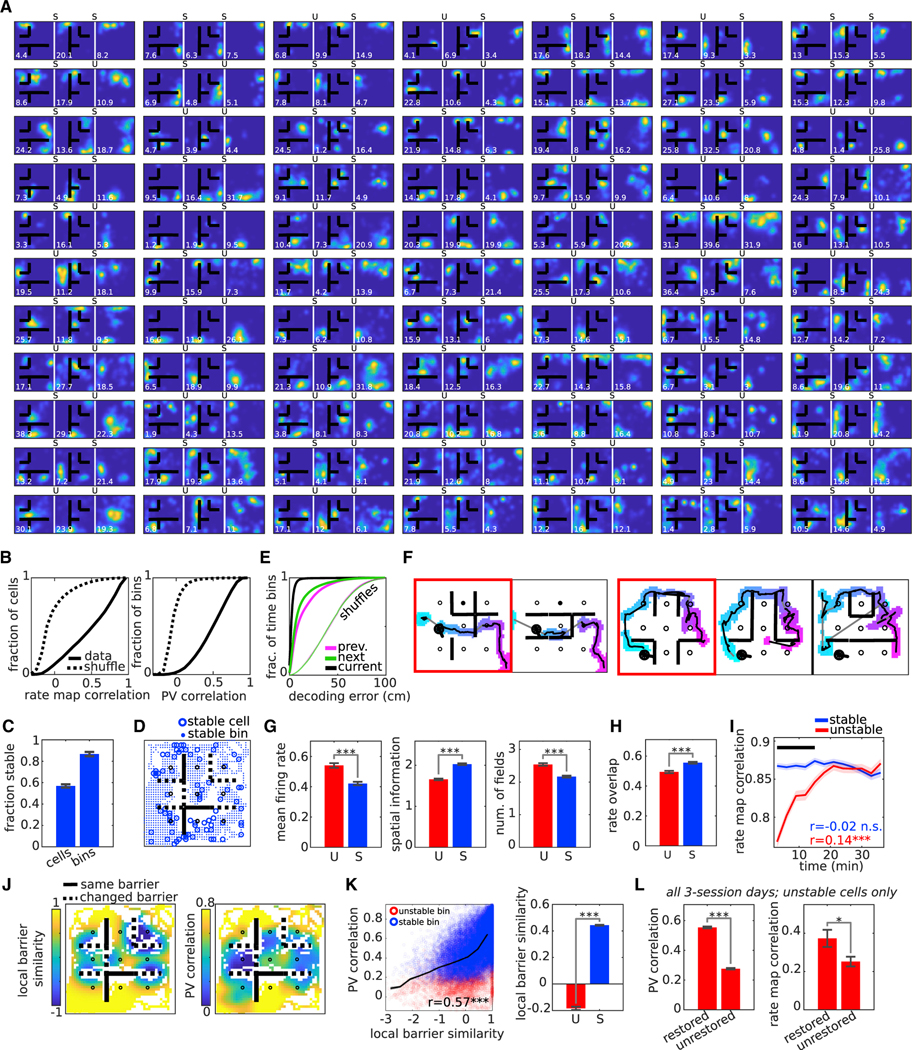
(A) Subset of rate maps for the same cells from sessions 79, 80, and 81 recorded on the same day from rat 1, ordered in descending order according to mean spatial information across sessions. Peak spatial firing rate (Hz/cm) at lower left of each panel. Stability of rate maps between neighboring sessions is indicated above each panel (S = stable cell, U = unstable cell).
(B) CDFs of the rate map correlations (left) and PV correlations (right). Rate map correlations were measured between the same cells across adjacent sessions recorded on the same day (n = 2,887, which is the total number of pairwise session measurements across all cells from rats 1–4; two-sample KS test, p < 0.001). PV correlations were measured between the same locations across adjacent sessions on the same day (n = 33,245, which is the total number of pairwise session measurements across all spatial bins from rats 1–4; two-sample KS test, p < 0.001). Only bins that were visited by the rat in both sessions are colored. Dashed lines: chance level from cell ID shuffle (two-sample KS tests, p < 0.001).
(C) Fractions of stable cells and stable bins across sessions are shown (n = 27, which is the total number of recorded adjacent session pairs from rats 1–4).
(D) Field peak locations and bin locations for all stable cells and stable bins, respectively, from session 80, rat 1. Solid (dashed) lines indicate overlapping (non-overlapping) barriers between the two sessions.
(E) Decoding error during run using the current (black), previous (magenta), or next (green) session place fields. Dashed lines, chance level from cell ID shuffle (two-sample KS tests, p < 0.001).
(F) Two example replays decoded with the place fields from different sessions recorded on the same day. The red box indicates during which session the replay occurred. Thus, in the first example at left, the replay occurred in session 1. The same replay decoded with the place fields from session 2 is shown in the neighboring box.
(G) Mean firing rate, spatial information, and number of fields for stable (S; n = 1,686) versus unstable (U; n = 1,201) cells.
(H) Rate overlap for stable versus unstable cells.
(I) Evolution of within-session rate map correlation in 6-min windows measured against the full session rate map for stable versus unstable cells. Horizontal black line, p < 0.05.
(J) Left: Local barrier similarity (LBS) between sessions 79 and 80, rat 1. Solid (dashed) lines same as in (D). Right: PV correlation map between sessions 79 and 80.
(K) Left: PV correlation versus LBS across all spatial bins of all session pairs (n = 33,245; Pearson’s r = 0.57, p < 0.001). Blue and red circles represent stable and unstable bins, respectively. Right: Mean local barrier similarity for stable (S; n = 28,788) versus unstable (U; n = 4,457) bins.
(L) Left: Mean PV correlation for “restored” bins (bins with low LBS scores across sessions 1 and 2 and high LBS scores across sessions 1–3; n = 1,374) versus “unrestored” bins (bins with low LBS scores across both sessions 1 and 2 and 1–3; n = 3,435) across all three-session days, using only the unstable cells (unstable between the first and second session of each day). Right: Same as left, except for rate map correlations between cells with rate maps in “restored” areas (cells with low cell barrier similarity (CBS; see STAR Methods) scores across sessions 1 and 2 and high CBS scores across sessions 1–3; n = 47) versus “unrestored” areas (cells with low CBS scores across both sessions 1 and 2 and 1–3; n = 133). Wilcoxon rank-sum tests; *p < 0.05, **p < 0.01, ***p < 0.001; error bars are SEM.
We next examined the properties of the unstable cells in our task. Compared to stable cells, unstable cells tended to have higher firing rates and more diffuse fields (Figure 5G), as well as higher instability in mean firing rate across sessions (Figure 5H). Moreover, field stabilization of the unstable cells occurred slowly over the course of the trial (Figure 5I) and was neither explained by any behavioral sampling bias (Figure S8E) nor mirrored by any obvious behavioral correlate (Figure S8F). To understand how field stability was impacted by the changes in the positions of the barriers, we created a measure of the similarity of the local environment across sessions (Figure 5J, left) and compared it to the PV correlations across different spatial locations (Figure 5J, right). PV correlations were highest at spatial bins near stable portions of the environment (Figure 5K). This was also true of the rate maps when calculated on a cell-by-cell basis (Figures S8G–S8I). We hypothesized that the observed instability was not random, but rather encoded the presence of barriers in the local environment. Thus, we predicted that cells that remap when the environment was locally changed (e.g., a barrier is removed in going from session 1 to session 2) should reinstate their original fields when the environment is locally restored (the barrier is returned to its original position in going from session 2 to session 3). For this analysis, we utilized the subset of recording days with 3 sessions. Indeed, we found that both the unstable-cell PV and rate map correlations exhibited a striking enhancement in stability around locations where the local environment was restored (Figure 5L; Figures S8J and S8K), suggesting that the unstable cells actually fire reliably to the presence (or absence) of local cues in the environment. Taken together, these results demonstrate the co-existence of two maps: a rigid place cell map in which the majority of cells participate, spatially invariant, rapidly instantiated and adapted, albeit imperfectly, to the new barrier configuration, and a slower-to-develop barrier-specific map that codes for local features of the environment (Figure S10A).
DISCUSSION
There has recently been increased interest in hippocampal replay as a general mechanism for learning and control, inspired by the rodent spatial literature (Wimmer et al., 2020; Schuck and Niv, 2019; Momennejad et al., 2018; Eldar et al., 2020; Liu et al., 2019; Mattar and Daw, 2018; Mnih et al., 2015; van de Ven and Tolias, 2018). A common theme is that replay reflects learned relationships between task states, be they locations or non-spatial states. However, most studies of replay in rodents have been restricted to very simple environments composed of tracks or open areas, so that the ability of replay to reflect arbitrary contingencies between states has barely been tested. Here we utilized a much more complex environment, which furthermore incorporated changes to goals and barrier structure between sessions, to reveal that replays did indeed depict traversable routes through the space reflecting the current contingencies between locations. Moreover, these depicted trajectories were predictive of future behavior, and were directed toward goals during phases of the task when such routes were needed.
Our results reveal a remarkable level of plasticity in replay sequences. Even after 90+ different barrier configurations, replay exhibited adaptation to each new configuration. By contrast, the underlying hippocampal representation was largely stable across different barrier configurations. The flexibility of the former, in contrast to the overall rigidity of the latter, is surprising given previous reports suggesting that place cells remap readily between different environments (Alme et al., 2014) and are sensitive to not just location but also events that happen in a location (Leutgeb et al., 2005), the origin and destination of routes through a location (Wood et al., 2000; Frank et al., 2000; Ferbinteanu and Shapiro, 2003), motivation (Moita et al., 2004; Kennedy and Shapiro, 2009), attention (Kentros et al., 2004; Muzzio et al., 2009; Monaco et al., 2014; Kelemen and Fenton, 2010), and minor changes in context (Muller and Kubie, 1987; Bostock et al., 1991). This propensity for remapping has led to the speculation that place cells are the readouts of memories stored in the hippocampus (Moser et al., 2015). However, remapping to encode context is not always observed (Berke et al., 2009; Ainge et al., 2012; Griffin and Hallock, 2013), and it has been noted that a general strategy of remapping to encode memory does not only provide a poor basis for generalization (Quian Quiroga, 2020) but leads to an unsustainable explosion in numbers of neurons needed in order to avoid catastrophic interference.
In line with this more critical view and consistent with our results, several studies have shown that place cells remain largely or entirely stable in tasks in which animals must make use of alternative routes when barriers are introduced to or manipulated within a familiar environment (Muller and Kubie, 1987; Rivard et al., 2004; Alvernhe et al., 2008, 2011; Duvelle et al., 2021). Such stability may reflect a place cell’s predisposition, possibly via its anatomical location (Danielson et al., 2016; Geiller et al., 2017), to ignore non-stationary or unpredictable cues in favor of idiothetic ones (Knierim et al., 1995; Sharp et al., 1995; Jeffery, 1998), though we did observe a substantial number of cells that, like object (Manns and Eichenbaum, 2009; Burke et al., 2011) or landmark vector (Deshmukh and Knierim, 2013; Sarel et al., 2017) cells, seemed to code for the barriers more explicitly (Rivard et al., 2004). Puzzlingly, accumulating evidence suggests that such tasks are dependent on the hippocampus (Thompson et al., 1984; Winocur et al., 2010; Rosenbaum et al., 2015), indicating that perhaps a more covert hippocampal mechanism is at play. Our results now point to replay and potentially other sequenced reactivations such as theta sequences (Foster and Wilson, 2007; Johnson and Redish, 2007; Wikenheiser and Redish, 2015) as the principal hippocampal mechanism by which the memory of the maze is read out to support flexible behavior. Furthermore, to the extent that our own experiences, like those of rats, vastly outnumber the places in which they occur, these results suggest a novel mechanism for the flexible creation and expression of memories in the brain.
How might the memory of the maze be encoded? One attractive possibility consistent with our data is that it is encoded within the hippocampus as synaptic changes to an otherwise rigid map or graph (Muller et al., 1996; Burgess and O’Keefe, 1996; Blum and Abbott, 1996; Gillner and Mallot, 1998; Redish and Touretzky, 1998; Whittington et al., 2020). This, in turn, could constrain the range and behavior of replays produced by the network (Figure S10). The rapid stabilization of the stable cells (Figure 5I) and the preservation of barrier avoidance with the stable cell time lag maps (Figure S8D), in conjunction with the rapid adaptation of replay (Figure 3E), supports this mechanism, at least early within the session. Specialized cell types like barrier-specific cells (Rivard et al., 2004), object or landmark vector cells (Manns and Eichenbaum, 2009; Burke et al., 2011; Deshmukh and Knierim, 2013; Sarel et al., 2017), interneurons (Stark et al., 2014), and boundary-encoding cells (Solstad et al., 2008; Lever et al., 2009) could then reinforce, refine, or even supplement the graph for the purposes of more accurate and more efficient navigation (Muller et al., 1996; Stachenfeld et al., 2017). Along these lines, the leaking of replays through barriers could be interpreted as a consequence of imperfectly adapted networks (Figure S9). On the other hand, Hopfield networks with “palimpsest” properties (Parisi, 1986; Chaudhuri and Fiete, 2016) solve the catastrophic interference problem by fading out older memories while at the same time flexibly encoding new ones, suggesting that replays that leak through the barriers may reflect more a feature of hippocampal processing than a bug. Alternatively, though not mutually exclusively, the maze may be encoded upstream in areas known to be involved in replay and sharp-wave ripples, including the ventral striatum (Lansink et al., 2009), ventral tegmental area (Gomperts et al., 2015; Valdé s et al., 2015), or cortex (Ji and Wilson, 2007; Jadhav et al., 2016; Berners-Lee et al., 2021). Untangling the roles of intra- versus extra-hippocampal mechanisms in the control and adaptation of replay is a question for future study.
STAR★METHODS
RESOURCE AVAILABILITY
Lead contact
Further information and requests for resources and reagents should be directed to and will be fulfilled by the Lead Contact, David Foster (davidfoster@berkeley.edu).
Materials availability
This study did not generate new unique reagents.
Data and code availability
All data reported in this paper will be shared by the lead contact upon request.
All original code has been deposited at Zenodo and is publicly available as of the date of publication. The DOI is listed in the key resources table.
Any additional information required to reanalyze the data reported in this work paper is available from the lead contact upon request.
KEY RESOURCES TABLE
| REAGENT or RESOURCE | SOURCE | IDENTIFIER |
|---|---|---|
| Experimental models: Organisms/strains | ||
|
| ||
| Rat: Crl:LE | Charles River | Strain Code: 006 |
|
| ||
| Software and algorithms | ||
|
| ||
| Mountainsort | Chung et al., 2017 | https://github.com/flatironinstitute/mountainsort |
| Trodes | Spike Gadgets | https://spikegadgets.com/ |
| Custom data processing and analysis code | This paper | Zenodo: https://doi.org/10.5281/zenodo.5880582 |
EXPERIMENTAL MODEL AND SUBJECT DETAILS
All experimental procedures were in accordance with the University of California Berkeley Animal Care and Use Committee and US National Institutes of Health guidelines. Neural activity was recorded from dorsal hippocampus (region CA1) of 4 Long-Evans rats (Rattus norvegicus; 3–4 months old) performing a goal-directed task in an open field maze with movable barriers (task described below). Rats were housed in a humidity and temperature controlled facility with a 12 h light-dark cycle. Before the start of the experiments, rats from the same breeding cohort were housed in pairs. At the start of the experiments, rats were single-housed.
METHOD DETAILS
Pre-training
Adult male Long-Evans wildtype rats (3–4 months old) were handled daily and put on a free-feeding diet for approximately 1 month. Pellets soaked in chocolate milk (Nesquik) were occasionally placed inside the rat’s cage to facilitate familiarity with the taste of chocolate. Rats were then food restricted to approximately 85%–90% of their free-feeding weight and then trained for 1 week on a linear track to drink chocolate milk from reward wells at both ends of the track.
Apparatus
The barrier maze was positioned at the center of a 10 by 10 ft room. The dimensions of the maze exterior were 90 by 90 cm. The maze floor was raised to a height of 52 cm off the floor. The perimeter of the maze consisted of plexiglass walls 60 cm high. The lower portion of each wall (up to 30 cm high) was painted with white geometrical designs (e.g., circles, cross-hatches, vertical parallel lines, etc) against a black background (Figure 1A). In addition, distinct geometrical cues hung from the distal walls of the room. The floor of the maze was made of a semi-absorbent material (cardboard spray-painted lightly with black latex paint) so as to preserve odor cues left by the rat. Between sessions, feces were removed from the floor and pools of urine were soaked up, but the floor was not wiped with ethanol. Rats were assigned separate floors (starting approximately 1–2 weeks after the start of training - before this, a cohort shared the same floor) in order to facilitate the familiarity with the environment. The floor contained 9 transparent conical reward wells 1.5 cm in diameter and evenly-spaced on a 3 by 3 grid, with an inter-well spacing of 23 cm along each dimension. Chocolate milk could be delivered in 0.1 mL amounts to each of the wells via a tubing system under the maze that was gated by solenoid valves controlled by the experimenter. The filling of wells elicited no obvious visual or auditory cues and lasted approximately 1 s. Green LEDs were placed under each well and programmed to flicker at 13 Hz when the well was filled (only on Random trials - see below). 6 jail bar-like barriers were constructed that could fit into any of 12 slots in the maze floor, yielding a total of unique barrier configurations (up to rotations). Each barrier was 19.5 cm (width) by 23 cm (height) and made of thin plexiglass rods (0.5 cm diameter) with an inter-rod spacing of 3.5 cm. Barriers were cleaned with ethanol between sessions. Rats were trained to avoid climbing over barriers.
Task design and training
The task consisted of alternate trials of goal-directed navigation to a fixed, unmarked Home well (Home trial) and cued navigation to one of the other 8 randomly baited Random wells (Random trial). Home wells were chosen pseudorandomly each session. The Random-well baiting sequence was controlled by the random number generator from an Arduino. On Random trials, the green LED beneath the baited random well flickered once the well was filled. Between trials, a 5–15 s random delay (controlled by an Arduino) was imposed between the end of drinking at the last well and the filling of the next well, in order to encourage better spatial coverage of the environment. Recording sessions typically lasted between 30 and 70 min, depending on the rat’s activity level. Room lights were kept dim for the duration of the session. During the session, the experimenter sat out of sight at a computer in the corner of the room. For each session, the positions of the 6 barriers were chosen pseudorandomly. The sequence of barrier configurations was approximately repeated across rats. During early training on the task, rats experienced one session per day. After a few days of training, the number of sessions per day was increased to 2, with an inter-session spacing of about 2–4 h. For two of the rats, the number of sessions per day was increased to 3, beginning a few weeks after surgery (Figure S1A). Between sessions, rats were returned to a sleep stand (an elevated glass dish inside a tall, well-lit cardboard box next to the recording computer) and neural activity was recorded for 1 h. Sometimes, rats were recorded for an additional hour before the next run. For longer intervals (greater than 2 h), the rats were returned to their home cage between recordings on the sleep stand. Rats did not experience a completely open maze (no barriers) until very late in the session sequence, if at all (Figure S1A).
Drive design and surgery
Four rats were implanted with microdrive arrays weighing 40–50 g and consisting of 64 independent-adjustable tetrodes made of twisted platinum iridium wires (Neuralynx) gold plated to an impedance of 150–300 MOhms. Drive cannulae were implanted bilaterally to target hippocampal dorsal CA1 (−4.13 AP, 2.68 ML relative to bregma) using a surgery protocol described elsewhere (Pfeiffer and Foster, 2013). Tetrodes were slowly lowered to the cell layer over the course of 2–4 weeks, which was identified by the presence (and shape) of strong-amplitude sharp-wave ripples. The rats were allowed 3–4 days recovery, after which behavioral training on the barrier maze task was resumed but without food restriction in their home cages. Food restriction was resumed a week after surgery.
Behavioral analysis
Rat position was tracked using automated software from Spike Gadgets and sampled at 30 Hz. Position and velocity were smoothed using a Butterworth filter (second order with a cutoff frequency of 0.1 samples/s using the butter function in MATLAB, selected to give reasonable smoothing to the rat’s trajectory). The beginning of each trial was marked as the time at which the rat had moved a distance of 6 cm away from the rewarded well after consuming the chocolate there. Drinking periods were defined as times in which the smoothed rat speed (a second order Butterworth filter with a cutoff frequency of 0.02 samples/s applied to the rat’s speed computed above), dropped below 1 cm/s while the rat was at the rewarded well. During bouts of anticipatory licking, rats exhibited characteristic speed and distance-to-well profiles (Figure S1B). Anticipatory licking periods were defined as times in which the rat was both near a well (within 6 cm) and the smoothed velocity stayed within 1–6 cm/s. The parameters listed above for the selection of the drinking and licking bouts as well as the need for secondary smoothing of the rat’s speed were determined so as to automate the process of bout demarcation so as to best match what would be selected manually.
To compute the probability of a well visit, a well was counted as visited on each trial if the rat came within 6 cm of it at least once. Well visit probability was then calculated in two ways, as a function of trial and collapsed across trials. For the former, well visit probability as a function of trial number was defined as the total number of times a particular well (Home versus Random) was visited on the ith trial divided by the total number of sessions. For the latter, well visit probability was defined as the total number of times a particular well was visited across trials divided by the total number of trials, then averaged across sessions. Only well visits that occurred within 5 s of the start of the trial and at least 1 s before the start of the drinking period were considered. The latter constraint was imposed so as to ensure that the behavior analyzed was unaffected by possible reward cues (i.e., the blinking light on Random trials, which could come on as early as 5 seconds after the beginning of the trial—see Task design and training). Only trials with duration less than 60 s were considered. For both the Random-well visit probabilities and Random-well anticipatory licking durations, data was averaged across all 8 Random wells of the session. For the Home well shuffle, the Home well was selected at random 10 times and the well visit probabilities were recomputed and averaged.
Cluster analysis
Spikes were extracted from channel LFP’s (sampled at 30 kHz) using Spike Gadgets Trodes software and clustered automatically using Mountainsort (Chung et al., 2017) and merged across sessions using the msdrift package. Additional cluster mergings across sessions was performed manually based on similarity of waveform. Clusters were accepted if noise overlap < 0.03, isolation > 0.95, peak SNR > 1.5 (Chung et al., 2017) and had passed a visual inspection.
Rate maps
For each spike time, the rat position and speed was found through linear interpolation (interp1 in MATLAB). Positions were binned with 2 cm square bins. The rate map for the cell was defined as
A speed cutoff of 5 cm/s was used in the construction of the rate maps to filter out spikes in which the rat was stationary or moving slowly. Smoothed rate maps were computed by first setting unvisited bins to zero and convolving the rate maps with a 2D isotropic Gaussian kernel (8 cm standard deviation (SD)). Spatial information (bits/spike) for the cell was defined as
where L is the number of spatial bins, is the probability of the rat being at the spatial bin, and is the cell’s mean firing rate. Place cells were identified as having r > 0.01 Hz and SI > 0.5 bits/sec. Field peak locations were measured as the spatial bin location with the highest firing rate. The number of fields for each rate map was calculated using a density-based clustering approach. First, rate maps were treated as discrete probability distributions and resampled 2,500 times (using the pinky function in MATLAB). Then, the sample points were clustered using dbscan in MATLAB, with a neighborhood search radius of 2.5 bins and a minimum number of neighbors of 50. The number of fields was set as the number of clusters found.
Rate map correlation
Rate map correlation was defined as the Pearson’s correlation between any pair of rate maps. For the cell, with rate maps and or the and sessions respectively, the rate map correlation was
where is the mean spatial firing rate. Rate map correlations were evaluated only at visited spatial bins common to both sessions and were only measured for cells identified as place cells for both sessions. A rate map correlation shuffle distribution was computed for each place cell by randomly permuting place cell ID’s 100 times in the second session and recomputing the correlations. A place cell was called stable across a pair of sessions if its rate map correlation exceeded the 95th percentile of its shuffle distribution; otherwise it was called unstable. A 2-tailed binomial test was performed to determine if the proportion of pairwise session correlation measurements across cells designated as stable was above chance level, assuming a chance level of stability of 50%. We note that the fraction of unstable cells measured in our task is probably an overestimate, given that some cells are likely to develop directional tuning in response to the linearization of the environment by the barriers. This, coupled with mismatched behavioral sampling across sessions, could lead to false rejections of stability. Rate overlap (Leutgeb et al., 2005) for the same place cell across a pair of sessions was computed by dividing the lower mean firing rate of the two sessions by the higher mean firing rate.
Within-session stability
Rate map correlation as a function of time within session was computed by first calculating rate maps within 6 min windows (shifted in 3-min increments) across the session (windowed rate maps). Rate map correlation was then computed between the windowed rate maps and the whole session rate map. Windowed rate maps for which there was insufficient behavioral sampling (i.e., less than 40% of all “active” spatial bins–bins with > 1 Hz firing rate–from the whole session rate map were visited by the rat during the 6 min window) were not analyzed. Field coverage fraction as a function of time within session was computed by calculating for each cell the fraction of the field covered by the rat within each 6 min window. Specifically, the fraction of the field covered was measured as the number of active bins within the place field visited by the rat divided by the total number of active bins. Position density correlation as a function of time within session was computed by correlating (Pearson’s) the rat position occupancy grid within each 6 min window against the full session position occupancy.
Population vector correlation
Population vectors (PVs) were constructed by concatenating the value of each place cell’s rate map at a given spatial bin into a vector. be the PV for the spatial bin, where N is the number of place cells. The PV correlation at the spatial bin across sessions I and J was computed as
where is the mean spatial firing rate at the bin across all place cells. PV correlations, like rate map correlations, were evaluated only at visited spatial bins common to both sessions and were only measured for cells identified as place cells andP having minimal overlap with the barriers in both sessions (see section on Rate map correlations). A PV correlation shuffle distribution was computed for each PV by randomly permuting place cell IDs 100 times in the second session and recomputing the PV correlations. A PV was called stable across a pair of sessions if the correlation exceeded the 95th percentile of its shuffle distribution. A 2-tailed binomial test was performed to determine if the proportion of pairwise session correlations across bins designated as stable was above chance level, assuming a chance level of stability of 50%. The binomial test was performed on PV correlations measured from coarse-grained rate maps (bin size = 4 cm) so as to reduce the otherwise inflated n-value used in the test.
Local barrier similarity
The barrier potential was computed for each barrier configuration by convolving the barriers with a 2D isotropic Gaussian kernel (24 cm SD) (Figure S5B). be the set of bins overlapping with the barriers in session I, where k indexes the overlapping bins, and , where K is the number of overlapping bins. The barrier potential at the spatial bin for session I was computed as
where h is the Gaussian kernel. The local barrier similarity (LBS) for the spatial bin across sessions I and J was defined as
where the summation is over the 6 closest spatial bins (indexed by l) to the bin and is the L2 norm. The cell barrier similarity (CBS) was the average local barrier similarity within the cell’s fields for sessions I and J. For the cell, this was defined as
where the summations are over the set of “active bins” in the cells field (bins with > 1 Hz firing rate) on sessions I and J (total number of active bins in sessions I and J is and , respectively).
Local barrier restoration and the reinstatement of rate maps and population vectors
For each 3-session day, “restored” spatial bins were selected that had low LBS on sessions 1–2 (i.e., the environment was changed locally) and high LBS on sessions 1–3 (i.e., the environment was restored locally). Specifically, the spatial bin was selected if and , where is the local barrier similarity of the spatial bin across sessions I and J and is the average LBS across all bins of all three sessions. In addition, the bin was required to have been visited by the rat in all three sessions. Likewise, ”unrestored” spatial bins were those bins that had both low LBS on sessions 1–2 and 1–3 (specifically, and for the bin). The population vector correlation across sessions 1–3 was then computed at the restored bins and unrestored bins using only cells designated as unstable between sessions 1–2 and active in all three sessions. Similarly, changes in rate map correlation as a function of local barrier restoration were computed by selecting cells with rate maps in “restored” areas (i.e., and , where is the cell barrier similarity of the cell across sessions I and J and is the average CBS across all cells of all three sessions) versus “unrestored” areas (i.e., and ). Again, only cells designated as unstable between sessions 1–2 and active in all three sessions were included in this analysis.
Spike density and sharp wave-ripple amplitude
Population spike density was computed by first summing the total number of spikes from all clusters in 1 ms non-overlapping time bins. Sharp wave-ripple amplitude was computed by band-pass filtering the LFP in the 120 to 170 Hz range and then extracting the amplitude envelope via a Hilbert transform. Both the spike density and ripple amplitude were smoothed through convolution with a Gaussian kernel (80 ms SD) and z-scored.
Bayesian decoding
Let be the number of spikes emitted by the place cell in a given time bin of duration . The posterior probability at bin conditioned on the activity vector (with the element as ) is given by Bayes rule (assuming Poisson spiking noise statistics, independence between neurons, and a uniform spatial prior (Davidson et al., 2009)):
A uniform prior was used for the purposes of making minimal assumptions about the location of the decoded positions. The posterior probability was computed for all bin locations where and L is the total number of spatial bins. Define and be the coordinates of the spatial bin. The coordinates of the posterior center-of-mass (COM) were given by
The posterior spread was defined as the square root of the second moment of the posterior:
The posterior COM jump size was defined as the L2 norm of the difference vector between consecutive posterior center-of-mass estimates: .
Replay detection and analysis
Classical approaches to extracting replay start with identifying population burst or sharp-wave ripple events and then evaluating the sequence content contained therein (Pfeiffer and Foster, 2013). In practice, we have found that many replay-like events during immobility periods were unaccompanied by large ripples or population bursts (Figure S2B). Thus, we developed a “bottom-up” procedure for replay extraction that wasn’t predicated on the existence of such events. Moreover, this technique allowed us to more flexibly and meaningfully demarcate replay boundaries. First, the Bayesian decoder was applied to spikes within a sliding window of 80 ms duration (shifted in 5 ms increments) over the entire session. We found that using a relatively large decoding window had little effect on the overall spatial structure of the replay (Figure S2F). Time bins were kept for further analysis based on three criteria: rat speed (; rat speed was computed at the center of each time bin via linear interpolation), posterior spread (m<10 cm), and posterior COM jumps size () (Figures S2A and S2B; see Bayesian decoding). We defined a subsequence as a set of temporally contiguous bins satisfying the above criteria. Subsequences captured epochs in which the posterior was well defined (small posterior spread) and moved smoothly (small COM jump size across time steps). Note that the jump size threshold was set to be relatively large to allow for barrier-crossing subsequences. The choice of the posterior spread threshold was set to be close to the “elbow” of the distribution (see Figures S2A and S2B). We next considered the possibility that long subsequences might get fragmented, for example when passing near a barrier. Thus, neighboring subsequences were merged if the spatial and temporal gap between them was 20 cm and 50 ms, respectively. This essentially imposed a velocity prior on the subsequence movement speed. A subsequence (merged or not) was denoted a candidate sequence if its duration was greater than 100 ms. We chose this duration threshold as it was roughly half of the mode of the replay duration distibution (~200 ms), Figures S2C and S2D. Replays were then selected as candidate events that were sufficiently spatially dispersed (so as to filter out any “stationary” replays—Denovellis et al., 2021). To this end, we defined a spatial dispersion metric:
where M is the number of time bins in the sequence and . A candidate sequence was defined as a replay if its dispersion was greater than 12 cm (Figure S2E). The dispersion threshold was set relatively low so as to be more permissive (see examples in Figure S3F) for the purposes of capturing possible shorter barrier-crossing replays.
Away-events were defined as replays that occurred during the drinking period at the Random well within the Random trial. Likewise, Home-events were defined as replays that occurred during the drinking period at the Home well within the Home trial. The probability of replay terminating at a well was computed as the number of trials in which a replay ended within 6 cm of the well divided by the total number of trials. For the Random well termination probability, data was averaged across all 8 Random wells of the session. For the Home well shuffle, the Home well was selected at random 10 times and the well termination probabilities were recomputed and averaged.
The angular displacement of replay relative to rat’s behavior was computed similar to previous work (Pfeiffer and Foster, 2013). be the location of the rat for a given replay (found via linear interpolation at the center of the event). For each time bin, a circle centered at was drawn that passes through the posterior center-of-mass estimate for that time bin, (Figure S2L). Angular displacements between and the intersections of the circle with the rat’s past and future trajectories were computed. If multiple intersections of the circle with the rat’s past or future trajectories, the intersection that occurred closest in time to the replay was used. We also computed the angular displacement between the intersection of the circle with the rat’s heading direction vector and the rat’s future trajectory. Absolute angular displacements within each class were averaged across the session. Only angular displacements for which cm were considered (Pfeiffer and Foster, 2013).
Decoding error during run
For the decoding error analysis in Figure 5E, posterior probabilities were calculated for non-overlapping time bins of 250 ms duration during running periods . Error was defined as the distance between the posterior center-of-mass estimate and the actual rat position in each time bin. For each session, a shuffle distribution for the error analysis was computed by shuffling place cell IDs 10 times and recomputing the error during run.
Replay vector field
For each spatial bin, the mean vector length and orientation (modulo 180 degrees) of the distribution of constituent replay vectors found within a radius of 2 spatial bins was computed. The modulo operation was used to collapse across orientations that differ by 180 degrees.
Barrier conformity analysis
Let be a constituent replay vector with unit length
where t takes values and M is the total number of time bins in the replay. The barrier conformity (BC) score for the constituent replay vector was defined as
where is the gradient of the barrier potential (see section Local Barrier Similarity) evaluated at the tail of each constituent replay vector ( Figure S5B). The first (second) term scores as high (low) constituent replay vectors perpendicular (parallel) to the local barrier potential gradient. We defined the session-averaged barrier conformity score as the average of all the BC scores across all replays in the session. In order to minimize bias in this calculation due to the uneven distribution of replays within the current environment, constituent replay vectors initiated within 4 cm of any of the twelve possible barrier positions were removed from the analysis before. Statistical significance of the score was determined by recomputing scores for the same dataset against all other 923 barrier configurations (“shuffle” distribution) and comparing with the test statistic. The p value was calculated as
where X is the number of shuffles greater than test statistic. The score was determined to be statistically significant if it exceeded the 95th percentile of its shuffle distribution (p < 0.05). A 2-tailed binomial test was performed to determine if the proportion of sessions with statistically significant scores was above chance level, assuming a chance level of significance of 50%.
The barrier conformity as a function of time within session was computed by averaging BC scores for all constituent replay vectors occurring within 6 min windows shifted in 3-min increments (Figure 3E). Time bins containing less than 200 constituent replay vectors were discarded. Scores were also computed against the previous barrier configuration (“previous”) or against all other possible barrier configurations (“shuffle”). Barrier conformity versus rat heading direction was computed by averaging all all BC scores for all constituent replay vectors occurring in front of (within an angle ± 90 degrees from the rat’s heading) versus behind the rat (within an angle ± 90 degrees opposite the rat’s heading) and at least 15 cm away (Figure S5D). For computing barrier conformity as a function of the distance to the nearest barrier, we defined a normalized barrier conformity score (Figure S5B) which normalizes the barrier potential gradient evaluated at each constituent replay vector to unit length (i.e., replace ) so as to remove the distance-to-barrier dependent discounting. Normalized barrier conformity scores were averaged across all constituent replay vectors occurring at a certain distance from the nearest barrier for each session. Distance bins containing less than 20 constituent replay vectors were discarded. For the shuffle, session scores were computed for each barrier configuration (except the current one) and then averaged.
Time-lag maps
To deal with the possibility that our inability to track replays in the vicinity of the barriers (because of the lack of place field coverage there) might lead us to erroneously conclude that replays avoid barriers, we devised an alternative method that did not require replay selection but instead using spikes from all candidate sequences. Let denote the posterior probability associated with the spatial bin at the time bin. The cross-correlogram of the posterior probability time series associated with the and spatial bins was computed by measuring cross-covariances at different lags, :
where T is the total number of time bins, is the lag, and is the temporal average over all time bins belonging to candidate events. Cross-covariances were computed for all temporal lags within the range of −1 to 1 s and smoothed through convolution with a Gaussian kernel (60 ms SD). Posterior probabilities were computed using a smaller decoding window of 20 ms in order to more reliably characterize the dynamics around the barriers. In computing the cross-covariances, posterior probabilities associated with time bins outside of candidate sequences or with above-threshold posterior spreads and COM jump sizes within candidate sequences (see Replay detection and analysis) were set to zero (note: candidate sequences were temporally demarcated using the original approach—with 80 ms decoding windows—as described above in Replay detection and analysis). For computational tractability, rate maps with larger spatial bins (4 cm square bins) were used. The time lag associated with a pair of bins was defined as
which extracts the absolute latency associated with the global peak in the cross-correlogram and then takes the absolute value. Time lags associated with unvisited spatial bins were removed.
Time-lag maps were constructed by arranging the time lags associated with a given spatial reference bin into a square grid. Thus, the column of the time lag matrix, , was defined as the time lag map for the spatial bin, when expanded into a 2D array. A time lag map slice was part of a row or column taken from a time lag map that starts at the reference bin and moves toward the nearest barrier along a path that intersects the barrier perpendicularly (Figure S6A). Time lag slices were averaged with the two nearest adjacent rows/columns, so as to avoid introducing potential artifacts by smoothing across the barrier. The distance between the reference bin and the nearest barrier location along the slice path was called the reference-bin-to-barrier distance. Each time lag map contributed at most one slice. For reference bins equidistant from two barriers, a slice was chosen randomly between the two directions. Slices for references bins close to the maze perimeter walls (less than 4 cm away) were excluded. Session-averaged slices were computed by averaging across all slices belonging to the same reference-bin-to-barrier distance class. The area under the slice was measured by numerically integrating each session-averaged slice (trapz in MATLAB) out to 8 bins (32 cm). As a control, slices were also taken from the same set of time lag maps assuming a barrier configuration complementary to the actual barrier configuration (i.e., the barriers occupy the other 6 positions within the environment). Time lag map slice analysis for the stable cells was performed by computing time lag maps using stable cells only. Since stability was defined with respect to the previous session, time lag maps were computed for all sessions except the first session of each day.
Multidimensional scaling (MDS) was applied to the time lag matrix in order to transform the temporal delays between pairs of spatial bins into spatial deformations between points on the Euclidean plane. First, the full time lag matrix was converted to a distance matrix by smoothing each time lag map with an 2D isotropic Gaussian kernel (1 bin SD), symmetrizing the matrix (by averaging the and elements), taking the log-transform (in order to discount longer time lags), and setting the diagonal to zero. A weight matrix was constructed of the same size and used to additionally weight elements of the distance matrix in the MDS algorithm: , where is the Euclidean distance between the and spatial bins, and bins. Multidimensional scaling was performed using mdscale in MATLAB, using the metricstress option, which uses the actual values of the dissimilarities (metric) that are then fitted by distances (stress) in the Euclidean plane. Lastly, Procrustes algorithm was applied (procrustes in MATLAB) to translate, rotate, and uniformly scale the set of bin positions in the Euclidean plane to best match the original positions of the bins before deformation (compare the left and right columns of Figure S6D). To demonstrate that the MDS algorithm was largely insensitive to missing data, MDS was applied to two sets of dissimilarity matrices corresponding to cityblock distances applied to an environment with and without barriers using the shortestpath function in MATLAB (Figures S6E and S6F).
Replay simulations
Replays were simulated using a bump attractor network where the movement of the bump was driven by spike-frequency adaptation (Hopfield, 2010; Itskov et al., 2011). Given a summed input current to the cell, the instantaneous firing rate of the cell was , with the neural transfer function f given by
Based on this time-varying input, neurons fired spikes according to a Poisson point process with a coefficient of variance of 1. The activation of synapses from the cell was given by
where is the synaptic time constant and
where specifies the time of the spike of the cell and the sum is over all spikes of the cell. We also implemented spike frequency adaptation. The adaptation dynamics for the cell was given by
where is the timescale of adaptation.
The total synaptic current into the cell was given by
where is the recurrent input (see below), is the adaptive inhibitory input ( is the strength of adaptation), is a small positive constant bias common to all cells, and is suppressive envelope function that tapers activity near the boundaries of the network (see below). The recurrent input was
where are the excitatory recurrent weights, is the strength of recurrent inhibitory feedback, and is the number of neurons in the network. To specify the recurrent weights, we first organized cells into a 2D array on the neural sheet (N neurons per dimension). be a set of translation-invariant weights with Gaussian shape that depend on the distance between cells in the neural sheet:
where xi is the cell’s location in the sheet and controls the spatial extent of the connectivity. mimics, for example, the resultant synaptic weights after Hebbian learning for a rat exploring a barrier-free environment assuming a one-to-one correspondence between the cell’s location in the neural sheet and the cell’s preferred firing location in the environment. To mimic synaptic weights learned in an environment with a barrier (Figures S9A and S9B), we drew an imaginary barrier line in the neural sheet corresponding to the barrier in the environment, then used the shortestpath function in MATLAB to compute the shortest paths between cells. We then used this distance metric, , to modulate the original translation-invariant weights :
The final recurrent weights were then a mixture of the original translation invariant weights and the barrier-respecting weights (Figure S9B), parameterized by the mixing ratio :
Lastly, the suppressive envelope function that tapers activity near the network edges (Burak and Fiete, 2009) was given by
where N is the size, per dimension, of the network, is the distance between the cell’s location in the neural sheet and the network edge, determines the range over which tapering occurs, and controls the steepness of the tapering.
For the simulations: the number of neurons per dimension was N = 32; timesteps were 0.5 ms; ; ; ; ; ; ; ; ; the duration of each simuation was 500 ms.
QUANTIFICATION AND STATISTICAL ANALYSIS
Statistical tests and corresponding p values are reported within the figure legends. All statistical analyses were performed in MATLAB. Wilcoxon sign-rank tests were used for paired comparisons and Wilcoxon rank-sum tests for nonpaired comparisons. Binomial tests were performed assuming 50% chance occurrences. Two-sample Kolmogorov-Smirnov tests were used to compare cumulative distributions of the data to chance. A minimum number of simultaneously recorded single units was a prerequisite for some analyses (analysis of replay). 3/4 rats were deemed to have sufficient cell yield in all recorded sessions for analysis (> 100 cells in all its sessions) and 1/4 rats was deemed not to (< 100 cells in all its sessions). This rat was used for place field analysis only.
Supplementary Material
Highlights.
Rats learn to solve a goal-directed navigation task with randomly-changing barriers.
Replay adapts to the new barriers and is predictive of future behavior.
Place fields are largely stable across barrier configurations.
ACKNOWLEDGMENTS
We would like to thank Yoram Burak, Ila Fiete, Andres Grosmark, Archit Gupta, Matt Kleinman, Will Liberti III, David Schwab, and Laurenz Wiskott for discussion, Rishi Chaudhuri for comments on the manuscript, and Charlie Walters for help on the drive design.
This work was supported by NIH grant NS113557. Animal use conformed to NIH guidelines and was approved by the UC Berkeley Animal Care and Use Committee.
Footnotes
SUPPLEMENTAL INFORMATION
Supplemental information can be found online at https://doi.org/10.1016/j.neuron.2022.02.002.
DECLARATION OF INTERESTS
The authors declare no competing interests.
REFERENCES
- Ainge JA, Tamosiunaite M, Wörgötter F, and Dudchenko PA (2012). Hippocampal place cells encode intended destination, and not a discriminative stimulus, in a conditional T-maze task. Hippocampus 22, 534–543. [DOI] [PubMed] [Google Scholar]
- Alme CB, Miao C, Jezek K, Treves A, Moser EI, and Moser M-B (2014). Place cells in the hippocampus: eleven maps for eleven rooms. Proc. Natl. Acad. Sci. USA 111, 18428–18435. [DOI] [PMC free article] [PubMed] [Google Scholar]
- Alvernhe A, Van Cauter T, Save E, and Poucet B (2008). Different CA1 and CA3 representations of novel routes in a shortcut situation. J. Neurosci. 28, 7324–7333. [DOI] [PMC free article] [PubMed] [Google Scholar]
- Alvernhe A, Save E, and Poucet B (2011). Local remapping of place cell firing in the Tolman detour task. Eur. J. Neurosci. 33, 1696–1705. [DOI] [PubMed] [Google Scholar]
- Alvernhe A, Sargolini F, and Poucet B (2012). Rats build and update topological representations through exploration. Anim. Cogn. 15, 359–368. [DOI] [PubMed] [Google Scholar]
- Bayne T, Brainard D, Byrne RW, Chittka L, Clayton N, Heyes C, Mather J, Ölveczky B, Shadlen M, Suddendorf T, and Webb B (2019). What is cognition? Curr. Biol. 29, R608–R615. [DOI] [PubMed] [Google Scholar]
- Berke JD, Breck JT, and Eichenbaum H (2009). Striatal versus hippocampal representations during win-stay maze performance. J. Neurophysiol. 101, 1575–1587. [DOI] [PMC free article] [PubMed] [Google Scholar]
- Berners-Lee A, Wu X, and Foster DJ (2021). Prefrontal cortical neurons are selective for non-local hippocampal representations during replay and behavior. J. Neurosci. 41, 5894–5908. [DOI] [PMC free article] [PubMed] [Google Scholar]
- Blum KI, and Abbott LF (1996). A model of spatial map formation in the hippocampus of the rat. Neural Comput. 8, 85–93. [DOI] [PubMed] [Google Scholar]
- Bostock E, Muller RU, and Kubie JL (1991). Experience-dependent modifications of hippocampal place cell firing. Hippocampus 1, 193–205. [DOI] [PubMed] [Google Scholar]
- Buja A, Swayne D, Littman M, Dean N, Hofmann H, and Chen L (2008). Data visualization with multidimensional scaling. J. Comput. Graph. Stat. 17, 444–472. [Google Scholar]
- Burak Y, and Fiete IR (2009). Accurate path integration in continuous attractor network models of grid cells. PLoS Comput. Biol. 5, e1000291. [DOI] [PMC free article] [PubMed] [Google Scholar]
- Burgess N, and O’Keefe J (1996). Cognitive graphs, resistive grids, and the hippocampal representation of space. J. Gen. Physiol. 107, 659–662. [DOI] [PMC free article] [PubMed] [Google Scholar]
- Burke SN, Maurer AP, Nematollahi S, Uprety AR, Wallace JL, and Barnes CA (2011). The influence of objects on place field expression and size in distal hippocampal CA1. Hippocampus 21, 783–801. [DOI] [PMC free article] [PubMed] [Google Scholar]
- Chaudhuri R, and Fiete I (2016). Computational principles of memory. Nat. Neurosci. 19, 394–403. [DOI] [PubMed] [Google Scholar]
- Chung JE, Magland JF, Barnett AH, Tolosa VM, Tooker AC, Lee KY, Shah KG, Felix SH, Frank LM, and Greengard LF (2017). A fully automated approach to spike sorting. Neuron 95, 1381–1394.e6. [DOI] [PMC free article] [PubMed] [Google Scholar]
- Danielson NB, Zaremba JD, Kaifosh P, Bowler J, Ladow M, and Losonczy A (2016). Sublayer-specific coding dynamics during spatial navigation and learning in hippocampal area CA1. Neuron 91, 652–665. [DOI] [PMC free article] [PubMed] [Google Scholar]
- Davidson TJ, Kloosterman F, and Wilson MA (2009). Hippocampal replay of extended experience. Neuron 63, 497–507. [DOI] [PMC free article] [PubMed] [Google Scholar]
- de Cothi W, Nyberg N, Griesbauer E-M, Ghanamé C, Zisch F, Lefort JM, Fletcher L, Newton C, Renaudineau S, Bendor D, et al. (2020). Predictive maps in rats and humans for spatial navigation: The successor representation explains flexible behaviour. bioRxiv. 10.1101/2020.09.26.314815. [DOI] [PMC free article] [PubMed]
- Denovellis EL, Gillespie AK, Coulter ME, Sosa M, Chung JE, Eden UT, and Frank LM (2021). Hippocampal replay of experience at real-world speeds. eLife 10, e64505. [DOI] [PMC free article] [PubMed] [Google Scholar]
- Deshmukh SS, and Knierim JJ (2013). Influence of local objects on hippocampal representations: Landmark vectors and memory. Hippocampus 23, 253–267. [DOI] [PMC free article] [PubMed] [Google Scholar]
- Diba K, and Buzsáki G (2007). Forward and reverse hippocampal place-cell sequences during ripples. Nat. Neurosci. 10, 1241–1242. [DOI] [PMC free article] [PubMed] [Google Scholar]
- Dupret D, O’Neill J, Pleydell-Bouverie B, and Csicsvari J (2010). The reorganization and reactivation of hippocampal maps predict spatial memory performance. Nat. Neurosci. 13, 995–1002. [DOI] [PMC free article] [PubMed] [Google Scholar]
- Duvelle É, Grieves RM, Hok V, Poucet B, Arleo A, Jeffery KJ, and Save E (2019). Insensitivity of place cells to the value of spatial goals in a two-choice flexible navigation task. J. Neurosci. 39, 2522–2541. [DOI] [PMC free article] [PubMed] [Google Scholar]
- Duvelle É, Grieves RM, Liu A, Jedidi-Ayoub S, Holeniewska J, Harris A, Nyberg N, Donnarumma F, Lefort JM, Jeffery KJ, et al. (2021). Hippocampal place cells encode global location but not connectivity in a complex space. Curr. Biol. 31, 1221–1233.e9. [DOI] [PMC free article] [PubMed] [Google Scholar]
- Ego-Stengel V, and Wilson MA (2010). Disruption of ripple-associated hippocampal activity during rest impairs spatial learning in the rat. Hippocampus 20, 1–10. [DOI] [PMC free article] [PubMed] [Google Scholar]
- Eichenbaum H (2004). Hippocampus: cognitive processes and neural representations that underlie declarative memory. Neuron 44, 109–120. [DOI] [PubMed] [Google Scholar]
- Eichenbaum H, and Cohen NJ (2014). Can we reconcile the declarative memory and spatial navigation views on hippocampal function? Neuron 83, 764–770. [DOI] [PMC free article] [PubMed] [Google Scholar]
- Eldar E, Lièvre G, Dayan P, and Dolan RJ (2020). The roles of online and offline replay in planning. eLife 9, e56911. [DOI] [PMC free article] [PubMed] [Google Scholar]
- Ferbinteanu J, and Shapiro ML (2003). Prospective and retrospective memory coding in the hippocampus. Neuron 40, 1227–1239. [DOI] [PubMed] [Google Scholar]
- Foster DJ (2017). Replay comes of age. Annu. Rev. Neurosci. 40, 581–602. [DOI] [PubMed] [Google Scholar]
- Foster DJ, and Wilson MA (2006). Reverse replay of behavioural sequences in hippocampal place cells during the awake state. Nature 440, 680–683. [DOI] [PubMed] [Google Scholar]
- Foster DJ, and Wilson MA (2007). Hippocampal theta sequences. Hippocampus 17, 1093–1099. [DOI] [PubMed] [Google Scholar]
- Frank LM, Brown EN, and Wilson M (2000). Trajectory encoding in the hippocampus and entorhinal cortex. Neuron 27, 169–178. [DOI] [PubMed] [Google Scholar]
- Geiller T, Fattahi M, Choi JS, and Royer S (2017). Place cells are more strongly tied to landmarks in deep than in superficial CA1. Nat. Commun. 8, 14531. 10.1038/ncomms14531. [DOI] [PMC free article] [PubMed] [Google Scholar]
- Gillner S, and Mallot HA (1998). Navigation and acquisition of spatial knowledge in a virtual maze. J. Cogn. Neurosci. 10, 445–463. [DOI] [PubMed] [Google Scholar]
- Girardeau G, Benchenane K, Wiener SI, Buzsá G, and Zugaro MB (2009). Selective suppression of hippocampal ripples impairs spatial memory. Nat. Neurosci. 12, 1222–1223. [DOI] [PubMed] [Google Scholar]
- Gomperts SN, Kloosterman F, and Wilson MA (2015). VTA neurons coordinate with the hippocampal reactivation of spatial experience. eLife 4, e05360. [DOI] [PMC free article] [PubMed] [Google Scholar]
- Griffin AL, and Hallock HL (2013). Hippocampal signatures of episodic memory: evidence from single-unit recording studies. Front. Behav. Neurosci. 7, 54. 10.3389/fnbeh.2013.00054. [DOI] [PMC free article] [PubMed] [Google Scholar]
- Gupta AS, van der Meer MA, Touretzky DS, and Redish AD (2010). Hippocampal replay is not a simple function of experience. Neuron 65, 695–705. [DOI] [PMC free article] [PubMed] [Google Scholar]
- Gustafson NJ, and Daw ND (2011). Grid cells, place cells, and geodesic generalization for spatial reinforcement learning. PLoS Comput. Biol. 7, e1002235. [DOI] [PMC free article] [PubMed] [Google Scholar]
- Hassabis D, Kumaran D, Vann SD, and Maguire EA (2007). Patients with hippocampal amnesia cannot imagine new experiences. Proc. Natl. Acad. Sci. USA 104, 1726–1731. [DOI] [PMC free article] [PubMed] [Google Scholar]
- Hebb DO, and Williams K (1946). A method of rating animal intelligence. J. Gen. Psychol. 34, 59–65. [DOI] [PubMed] [Google Scholar]
- Hopfield JJ (2010). Neurodynamics of mental exploration. Proc. Natl. Acad. Sci. USA 107, 1648–1653. [DOI] [PMC free article] [PubMed] [Google Scholar]
- Itskov V, Curto C, Pastalkova E, and Buzsáki G (2011). Cell assembly sequences arising from spike threshold adaptation keep track of time in the hippocampus. J. Neurosci. 31, 2828–2834. [DOI] [PMC free article] [PubMed] [Google Scholar]
- Jadhav SP, Kemere C, German PW, and Frank LM (2012). Awake hippocampal sharp-wave ripples support spatial memory. Science 336, 1454–1458. [DOI] [PMC free article] [PubMed] [Google Scholar]
- Jadhav SP, Rothschild G, Roumis DK, and Frank LM (2016). Coordinated excitation and inhibition of prefrontal ensembles during awake hippocampal sharp-wave ripple events. Neuron 90, 113–127. [DOI] [PMC free article] [PubMed] [Google Scholar]
- Jeffery KJ (1998). Learning of landmark stability and instability by hippocampal place cells. Neuropharmacology 37, 677–687. [DOI] [PubMed] [Google Scholar]
- Ji D, and Wilson MA (2007). Coordinated memory replay in the visual cortex and hippocampus during sleep. Nat. Neurosci. 10, 100–107. [DOI] [PubMed] [Google Scholar]
- Johnson A, and Redish AD (2007). Neural ensembles in CA3 transiently encode paths forward of the animal at a decision point. J. Neurosci. 27, 12176–12189. [DOI] [PMC free article] [PubMed] [Google Scholar]
- Kabadayi C, Bobrowicz K, and Osvath M (2018). The detour paradigm in animal cognition. Anim. Cogn. 21, 21–35. [DOI] [PMC free article] [PubMed] [Google Scholar]
- Kelemen E, and Fenton AA (2010). Dynamic grouping of hippocampal neural activity during cognitive control of two spatial frames. PLoS Biol. 8, e1000403. [DOI] [PMC free article] [PubMed] [Google Scholar]
- Kennedy PJ, and Shapiro ML (2009). Motivational states activate distinct hippocampal representations to guide goal-directed behaviors. Proc. Natl. Acad. Sci. USA 106, 10805–10810. [DOI] [PMC free article] [PubMed] [Google Scholar]
- Kentros CG, Agnihotri NT, Streater S, Hawkins RD, and Kandel ER (2004). Increased attention to spatial context increases both place field stability and spatial memory. Neuron 42, 283–295. [DOI] [PubMed] [Google Scholar]
- Knierim JJ, Kudrimoti HS, and McNaughton BL (1995). Place cells, head direction cells, and the learning of landmark stability. J. Neurosci. 15, 1648–1659. [DOI] [PMC free article] [PubMed] [Google Scholar]
- Kohler W (1925). The mentality of apes (Harcourt, Brace & World; ). [Google Scholar]
- Komorowski RW, Manns JR, and Eichenbaum H (2009). Robust conjunctive item-place coding by hippocampal neurons parallels learning what happens where. J. Neurosci. 29, 9918–9929. [DOI] [PMC free article] [PubMed] [Google Scholar]
- Lansink CS, Goltstein PM, Lankelma JV, McNaughton BL, and Pennartz CMA (2009). Hippocampus leads ventral striatum in replay of place-reward information. PLoS Biol. 7, e1000173. [DOI] [PMC free article] [PubMed] [Google Scholar]
- Leutgeb JK, Leutgeb S, Treves A, Meyer R, Barnes CA, McNaughton BL, Moser M-B, and Moser EI (2005). Progressive transformation of hippocampal neuronal representations in “morphed” environments. Neuron 48, 345–358. [DOI] [PubMed] [Google Scholar]
- Lever C, Burton S, Jeewajee A, O’Keefe J, and Burgess N (2009). Boundary vector cells in the subiculum of the hippocampal formation. J. Neurosci. 29, 9771–9777. [DOI] [PMC free article] [PubMed] [Google Scholar]
- Liu Y, Dolan RJ, Kurth-Nelson Z, and Behrens TEJ (2019). Human replay spontaneously reorganizes experience. Cell 178, 640–652.e14. [DOI] [PMC free article] [PubMed] [Google Scholar]
- Maguire EA, Nannery R, and Spiers HJ (2006). Navigation around London by a taxi driver with bilateral hippocampal lesions. Brain 129, 2894–2907. [DOI] [PubMed] [Google Scholar]
- Manns JR, and Eichenbaum H (2009). A cognitive map for object memory in the hippocampus. Learn. Mem. 16, 616–624. [DOI] [PMC free article] [PubMed] [Google Scholar]
- Mattar MG, and Daw ND (2018). Prioritized memory access explains planning and hippocampal replay. Nat. Neurosci. 21, 1609–1617. [DOI] [PMC free article] [PubMed] [Google Scholar]
- Mnih V, Kavukcuoglu K, Silver D, Rusu AA, Veness J, Bellemare MG, Graves A, Riedmiller M, Fidjeland AK, Ostrovski G, et al. (2015). Human-level control through deep reinforcement learning. Nature 518, 529–533. [DOI] [PubMed] [Google Scholar]
- Moita MAP, Rosis S, Zhou Y, LeDoux JE, and Blair HT (2003). Hippocampal place cells acquire location-specific responses to the conditioned stimulus during auditory fear conditioning. Neuron 37, 485–497. [DOI] [PubMed] [Google Scholar]
- Moita M, Rosis S, Zhou Y, LeDoux JE, and Blair HT (2004). Putting fear in its place: remapping of hippocampal place cells during fear conditioning. J. Neurosci. 24, 7015–7023. [DOI] [PMC free article] [PubMed] [Google Scholar]
- Momennejad I, Otto AR, Daw ND, and Norman KA (2018). Offline replay supports planning in human reinforcement learning. eLife 7, e32548. [DOI] [PMC free article] [PubMed] [Google Scholar]
- Monaco JD, Rao G, Roth ED, and Knierim JJ (2014). Attentive scanning behavior drives one-trial potentiation of hippocampal place fields. Nat. Neurosci. 17, 725–731. [DOI] [PMC free article] [PubMed] [Google Scholar]
- Morris RG, Garrud P, Rawlins JN, and O’Keefe J (1982). Place navigation impaired in rats with hippocampal lesions. Nature 297, 681–683. [DOI] [PubMed] [Google Scholar]
- Moser M-B, Rowland DC, and Moser EI (2015). Place cells, grid cells, and memory. Cold Spring Harb. Perspect. Biol. 7, a021808. [DOI] [PMC free article] [PubMed] [Google Scholar]
- Muller RU, and Kubie JL (1987). The effects of changes in the environment on the spatial firing of hippocampal complex-spike cells. J. Neurosci. 7, 1951–1968. [DOI] [PMC free article] [PubMed] [Google Scholar]
- Muller RU, Stead M, and Pach J (1996). The hippocampus as a cognitive graph. J. Gen. Physiol. 107, 663–694. [DOI] [PMC free article] [PubMed] [Google Scholar]
- Muzzio IA, Levita L, Kulkarni J, Monaco J, Kentros C, Stead M, Abbott LF, and Kandel ER (2009). Attention enhances the retrieval and stability of visuospatial and olfactory representations in the dorsal hippocampus. PLoS Biol. 7, e1000140. [DOI] [PMC free article] [PubMed] [Google Scholar]
- O’Keefe J, and Nadel L (1978). The hippocampus as a cognitive map (Oxford: Clarendon Press; ). [Google Scholar]
- Ólafsdottir HF, Barry C, Saleem AB, Hassabis D, and Spiers HJ (2015). Hippocampal place cells construct reward related sequences through unexplored space. eLife 4, e06063. [DOI] [PMC free article] [PubMed] [Google Scholar]
- Parisi G (1986). A memory which forgets. J. Phys. A. 19, L617. [Google Scholar]
- Pfeiffer BE, and Foster DJ (2013). Hippocampal place-cell sequences depict future paths to remembered goals. Nature 497, 74–79. [DOI] [PMC free article] [PubMed] [Google Scholar]
- Quian Quiroga R (2020). No pattern separation in the human hippocampus. Trends Cogn. Sci. 24, 994–1007. [DOI] [PubMed] [Google Scholar]
- Rashotte ME (1987). Behavior in relation to objects in space: Some historical perspectives. In Cognitive processes and spatial orientation in animal and man, Volume 36, Ellen P and Thinus-Blanc C, eds. (Dordrecht: Springer; ), pp. 39–54. [Google Scholar]
- Redish AD, and Touretzky DS (1998). The role of the hippocampus in solving the Morris water maze. Neural Comput. 10, 73–111. [DOI] [PubMed] [Google Scholar]
- Rivard B, Li Y, Lenck-Santini P-P, Poucet B, and Muller RU (2004). Representation of objects in space by two classes of hippocampal pyramidal cells. J. Gen. Physiol. 124, 9–25. [DOI] [PMC free article] [PubMed] [Google Scholar]
- Rosenbaum RS, Cassidy BN, and Herdman KA (2015). Patterns of preserved and impaired spatial memory in a case of developmental amnesia. Front. Hum. Neurosci. 9, 196. 10.3389/fnhum.2015.00196. [DOI] [PMC free article] [PubMed] [Google Scholar]
- Sarel A, Finkelstein A, Las L, and Ulanovsky N (2017). Vectorial representation of spatial goals in the hippocampus of bats. Science 355, 176–180. [DOI] [PubMed] [Google Scholar]
- Schuck NW, and Niv Y (2019). Sequential replay of nonspatial task states in the human hippocampus. Science 364, eaaw5181. [DOI] [PMC free article] [PubMed] [Google Scholar]
- Sharp PE, Blair HT, Etkin D, and Tzanetos DB (1995). Influences of vestibular and visual motion information on the spatial firing patterns of hippocampal place cells. J. Neurosci. 15, 173–189. [DOI] [PMC free article] [PubMed] [Google Scholar]
- Smith DM, and Mizumori SJ (2006). Hippocampal place cells, context, and episodic memory. Hippocampus 16, 716–729. [DOI] [PubMed] [Google Scholar]
- Solstad T, Boccara CN, Kropff E, Moser M-B, and Moser EI (2008). Representation of geometric borders in the entorhinal cortex. Science 322, 1865–1868. [DOI] [PubMed] [Google Scholar]
- Stachenfeld KL, Botvinick MM, and Gershman SJ (2017). The hippocampus as a predictive map. Nat. Neurosci. 20, 1643–1653. [DOI] [PubMed] [Google Scholar]
- Stark E, Roux L, Eichler R, Senzai Y, Royer S, and Buzsáki G (2014). Pyramidal cell-interneuron interactions underlie hippocampal ripple oscillations. Neuron 83, 467–480. [DOI] [PMC free article] [PubMed] [Google Scholar]
- Thompson R, Harmon D, and Yu J (1984). Detour problem-solving behavior in rats with neocortical and hippocampal lesions: A study of response flexibility. Physiol. Psychol. 12, 116–124. [Google Scholar]
- Tolman EC (1948). Cognitive maps in rats and men. Psychol. Rev. 55, 189–208. [DOI] [PubMed] [Google Scholar]
- Valdés JL, McNaughton BL, and Fellous JM (2015). Offline reactivation of experience-dependent neuronal firing patterns in the rat ventral tegmental area. J. Neurophysiol. 114, 1183–1195. [DOI] [PMC free article] [PubMed] [Google Scholar]
- van de Ven G and Tolias A (2018). Generative replay with feedback connections as a general strategy for continual learning. Preprint at arXiv: 1809.10635. [Google Scholar]
- Whittington JCR, Muller TH, Mark S, Chen G, Barry C, Burgess N, and Behrens TEJ (2020). The Tolman-Eichenbaum machine: Unifying space and relational memory through generalization in the hippocampal formation. Cell 183, 1249–1263.e23. [DOI] [PMC free article] [PubMed] [Google Scholar]
- Wikenheiser AM, and Redish AD (2015). Hippocampal theta sequences reflect current goals. Nat. Neurosci. 18, 289–294. [DOI] [PMC free article] [PubMed] [Google Scholar]
- Wimmer GE, Liu Y, Vehar N, Behrens TEJ, and Dolan RJ (2020). Episodic memory retrieval success is associated with rapid replay of episode content. Nat. Neurosci. 23, 1025–1033. [DOI] [PMC free article] [PubMed] [Google Scholar]
- Winocur G, Moscovitch M, and Bontempi B (2010). Memory formation and long-term retention in humans and animals: convergence towards a transformation account of hippocampal-neocortical interactions. Neuropsychologia 48, 2339–2356. [DOI] [PubMed] [Google Scholar]
- Wood ER, Dudchenko PA, Robitsek RJ, and Eichenbaum H (2000). Hippocampal neurons encode information about different types of memory episodes occurring in the same location. Neuron 27, 623–633. [DOI] [PubMed] [Google Scholar]
Associated Data
This section collects any data citations, data availability statements, or supplementary materials included in this article.
Supplementary Materials
Data Availability Statement
All data reported in this paper will be shared by the lead contact upon request.
All original code has been deposited at Zenodo and is publicly available as of the date of publication. The DOI is listed in the key resources table.
Any additional information required to reanalyze the data reported in this work paper is available from the lead contact upon request.
KEY RESOURCES TABLE
| REAGENT or RESOURCE | SOURCE | IDENTIFIER |
|---|---|---|
| Experimental models: Organisms/strains | ||
|
| ||
| Rat: Crl:LE | Charles River | Strain Code: 006 |
|
| ||
| Software and algorithms | ||
|
| ||
| Mountainsort | Chung et al., 2017 | https://github.com/flatironinstitute/mountainsort |
| Trodes | Spike Gadgets | https://spikegadgets.com/ |
| Custom data processing and analysis code | This paper | Zenodo: https://doi.org/10.5281/zenodo.5880582 |