Out-of-focus brain image detection in serial tissue sections

Abstract

Background:

A large part of image processing workflow in brain imaging is quality control which is typically done visually. One of the most time consuming steps of the quality control process is classifying an image as in-focus or out-of-focus (OOF).

New method:

In this paper we introduce an automated way of identifying OOF brain images from serial tissue sections in large datasets (> 1.5 PB). The method utilizes steerable filters (STF) to derive a focus value (FV) for each image. The FV combined with an outlier detection that applies a dynamic threshold allows for the focus classification of the images.

Results:

The method was tested by comparing the results of our algorithm with a visual inspection of the same images. The results support that the method works extremely well by successfully identifying OOF images within serial tissue sections with a minimal number of false positives.

Comparison with existing methods: Our algorithm was also compared to other methods and metrics and successfully tested in different stacks of images consisting solely of simulated OOF images in order to demonstrate the applicability of the method to other large datasets.

Conclusions:

We have presented a practical method to distinguish OOF images from large datasets that include serial tissue sections that can be included in an automated pre-processing image analysis pipeline.

1. Introduction

The development of whole slide imaging (WSI), that allows for the digitization of entire histologic samples using high-resolution scanning, is becoming an invaluable tool in diagnosis of a large variety of diseases (Barker et al., 2016; Saco et al., 2017; Mukhopadhyay et al., 2018). There are enormous advantages in using this new modality for diagnostics, research and education. Entire slides of samples can be shared, accessed and evaluated by different groups. However, massive file sizes of the resulting images can create storage and processing challenges (Farahani et al., 2015). Fortunately, modern computers can facilitate the collection and archiving of those data but at the same time the need for automated analysis tools arises.

Brain imaging is one of the many fields that benefits from the advent of whole slide imaging. Our datasets are part of Cold Spring Harbor Laboratory’s (CSHL) Mouse Brain Architecture (MBA) project. The goal of the project is to map the mouse brain at a mesoscopic scale so that we can explore the neural connections between the different parts of the brain (Bohland et al., 2009). When observing the brain at the microscopic scale there is a great degree of variability due to the large number of neurons while at the macroscopic level the patterns are relatively stable within each species. By using different tracers to highlight the different brain sections, we can study the circuit architecture of entire mice brains. Because of variability in brain shape and size of the different mice, we have to repeat the imaging numerous times using various samples. This creates a massive amount of images with a staggering amount of detail and complexity.

A large part of the image processing workflow in brain imaging is the quality control which is typically done visually. During this process, the different images are evaluated visually and images that are not deemed optimal are identified. There are many characteristics that must be identified; for instance, whether the images are damaged, folded, contain noise or artifacts. Distinguishing these image properties can be accomplished quickly and accurately through visual inspection. Examples of such images are shown in Figures 1a, 1d, 1g.

Figure 1:

Examples of different fluorescent (first row), Nissl stained (second row), immunohistochemistry stained images (third row) from our datasets. Images (a), (d), (g) depict an image with an artifact on the sample, air bubbles on the folded sample and a damaged image respectively. OOF images are presented in (b), (e), (h), while in-focus images are shown in (c), (f) and (i). Note that our images and included samples are not all the same size and the samples are not always centered in the image.

Another important, yet time consuming, step of the quality control process is classifying whether an image is in-focus or out-of-focus (OOF). The digital scanner used to digitize slides may result in images that are OOF despite being equipped with an autofocus system. In the process of imaging a three dimensional tissue sample into a two dimensional image, the autofocus system may fail to select the appropriate focus points which can result in OOF images.

Classifying an image as OOF is not only time consuming but it depends on the observer’s skills. There are many images that are clearly OOF (Figures 1b, 1e, 1h), which can be characterized as such with high confidence by any observer. However, some images can be either slightly OOF (Figure 2) or partially OOF (Figure 3). Both cases can be time consuming as a magnified view of smaller tiles of the image have to be examined in order to determine the focus of each image. Examining partially OOF images also requires a skilled observer to evaluate every small tile of an image to assure that no OOF region is missed. Both cases can be lengthy and laborious and the skill of the observer will determine whether the identification of OOF images is complete and accurate. Utilizing an automated way to identify the OOF images will improve the speed of the analysis and avoid mistakes that can be introduced due to human error or lack of skills and experience.

Figure 2:

Example of fluorescent image that is OOF when magnified. The image in full view does not look OOF but once the image is magnified (A and B) the image is clearly OOF. A magnified view of a similar area from a different image that is not OOF is included (C) for comparison.

Figure 3:

Example of fluorescent image that is partially OOF. We have magnified two regions of interest from the same image. It is shown that, even though both regions are from the same image, the upper region (A) is OOF while the lower region (B) is in-focus.

We are presenting an automated focus classification method using data from the Mouse Brain Architecture project. Locating the OOF images is important because their inclusion in the dataset can significantly affect the quality of subsequent analyses such as cell segmentation. The project is generating data with a Hamamatsu NanoZoomer 2.0 HT automated slide scanning microscope, but this methodology can be used with other scanners that digitize brain images, as well as images from different fields. The automated way of identifying OOF images that is presented in this work eliminates the dependency on the observer’s skills, automates the process and greatly accelerates the inspection.

Our application concerns the focus assessment of the image datasets after the imaging is completed with the purpose of identifying the OOF samples, repeating the scanning for the particular images and then replacing them with the new in-focus images. Previous approaches to this problem can be grouped into two general categories: estimation of a metric with OOF identification based on a threshold or score and machine learning approaches. The first category has the disadvantage of requiring a threshold that can be determined using a subjective classification (Bray et al., 2012; Bray & Carpenter, 2017). Such a method might not be appropriate when an automated method is employed because inserting a threshold that has to be empirically determined might not allow for the algorithm to run without human intervention. Additionally, due to the differences in illumination, modalities and stains of each individual dataset, determining such a threshold would be very challenging and error-prone. Using neural networks to identify OOF images has also been explored in cell imaging and digital pathology samples (Yang et al., 2018; Senaras et al., 2018). In order for such methods to be implemented on our datasets, training image datasets have to be synthesized with added noise that mimics the actual OOF images because of imbalanced classes in each series (the fraction of OOF images for each stack is very small for the majority of stacks). But such modeling can be challenging due to the large variety of structure sizes, image modalities and stains in our images, as well as the complexity of simulating the real blurring and noise effects that we observe in our images. Additionally we do not have the ability to scan slides on different focal planes which will make our training sample of OOF images small since the OOF images are always a small percentage compared with all the images.

2. Materials and methods

2.1. Description of the brain dataset

The datasets used are serial brain tissue sections of different samples that are part of the MBA project. The whole brain of each mouse is cut into slices of approximately 20μm thickness after it has been frozen (Pinskiy et al., 2013). The different sections are mounted onto glass slides and each slice is digitally imaged (Pinskiy et al., 2015) with a scanner that works in lanes. Each of these images is two dimensional and the brain can be reconstructed in three dimensions by stacking all the images of the same brain together. Because of variability in brain shape and size of the different mice, the above procedure is repeated with numerous samples.

The resulting images have very high resolution and the entire dataset is larger than 1.5 PB. Each complete brain is made up of a “stack” of approximately 600 images (with alternating sections of Nissl stain and tracers). The inputs and outputs of the brain regions are traced using anterograde (adeno-associated virus - AAV) and retrograde tracers (Cholera toxin subunit B - CTB). The tracers are depicted either with a fluorescent label (AAV) or a histochemical label and bright-field imaging (CTB) (Mitra, 2014). Fluorescence (F) is useful because it enhances the contrast of the cells with their neighbors. Fluorescence series were scanned using a tri-filter cube (FITC/TX-RED/DAPI) so that three color channels (RGB) per slide could be obtained. An X-Cite light source (Lumen Dynamics) was used to produce the excitation fluorescence. In this paper, Nissl stained images are denoted as N images while immunohistochemistry stained images are denoted as IHC images. All scanning is performed using a 20X objective (0.46μm per pixel) and each image is close to 1 billion pixels. For instance, an image of this size would represent an area of approximately 14 mm on each side, with the tissue sample typically occupying an area between 10%–80% of the entire image. The amount of detail in the images makes the project challenging because any analysis performed on these images pushes the computational limits that are available.

2.2. Analysis

The classification method consists of the sample edge detection, focus metric calculation and outlier detection. Appendix C represents a flowchart of our proposed method.

2.2.1. Edge detection.

The images contain the brain tissue and a large background area without a sample. Cropping the background facilitates faster image analysis due to the smaller size of the images and removes any background artifacts that could hinder an accurate focus calculation.

The first step of the edge detection algorithm is applying a median filter to remove any noise or specks to overcome detecting false edges. The size of the median filter is usually determined empirically as it has to balance two requirements; the kernel size has to be large enough to reduce the noise but must also be small enough to retain the sharpness of the tissue edges so that these edges can be located by the edge detection operator. A common kernel size can be used for images that are taken using the same experimental setup and we have used a 7 × 7 pixel kernel for this particular dataset. Implementing a Sobel filter (Gonzalez & Woods, 2006) allows us to reveal the edges of the images as the Sobel operator emphasizes the regions of high frequency. In real world images, such as the ones presented in this paper, the background can include artifacts, shadows or noise which could make distinguishing the tissue edges from other features challenging. The enhanced edges from the filtered image are connected using dilation and the different regions are filled. The largest closed region is considered the brain structure and its pixel coordinates are used to create a tissue mask. We utilized several built-in MATLAB (MATLAB, 2018) functions for these operations, such as medfilt2, edge, imdilate, imfill and bwboundaries.

Other methods for edge detection such as the Canny filter (Canny, 1986), Prewitt operator (Prewitt, 1970), Roberts cross operator (Roberts, 1963) and Otsu’s thresholding (Otsu, 1979) were also tested. Although all the different methods yielded satisfactory results for most images, all methods except the Sobel filter failed to detect the tissue edges of many images that were OOF. Since the goal of the project is to detect the OOF images, it is important to achieve proper edge detection in all groups of images, therefore the Sobel filter was the appropriate filter to apply for edge detection.

2.2.2. Focus metric description

The focus measure we used to classify the images is based on the use of steerable filters (STF) (Minhas et al., 2009; Freeman & Adelson, 1991). Although STF have been used to estimate the depth map for shape reconstruction (Minhas et al., 2012) and the calculation of robust focus measure functions for individual images (Shah et al., 2017), to the authors’ knowledge, they have not been used to evaluate the focus in real world serial tissue sections for the purpose of identifying OOF images. We have created a novel classification scheme based on a focus value derived from the application of STF in each image and an outlier detection with a dynamic threshold.

Filters with arbitrary orientations synthesized using a linear combination of the basis filters, are used to find the response for each image pixel and calculate a figure of merit that we will later call a focus value (FV). An image can be considered as a function where f(x, y) is its intensity at position/pixel (x, y). If the image data points are an array of samples of a continuous function of the image intensity, then the gradient is a measure of change of that function. First, a Gaussian mask must be created in order to filter the image.

The 2D Gaussian kernel is defined as:

$$G(x,y)=\frac{1}{2\pi {\sigma }^2}{e}^{-\frac{(x^2+y^2)}{2{\sigma }^2}}$$ (1)

The partial derivatives of Eq. (1) are:

$$G_x=\frac{\partial f}{\partial x}=-\frac{x}{{\sigma }^2}G(x,y)$$ (2)

$$G_y=\frac{\partial f}{\partial y}=-\frac{y}{{\sigma }^2}G(x,y)$$ (3)

It can be noted that Eq. (3) is the same function as Eq. (2) rotated by 90°. The previous two filters can be used as basis filters in order to construct filters of an arbitrary orientation angle θ. A new filter of an arbitrary orientation can be constructed by the linear combination of these two filters.

$$G_{\theta }=\cos (\theta )G_x+\sin (\theta )G_y$$ (4)

In a region of the image that has a high intensity variation the steerable filters will respond with large amplitude for a proper orientation whereas in a poorly selected orientation the same region would have low intensity variation. In order to find the maximum response of each individual pixel of the image, which will correspond to a pixel that has the largest intensity difference between neighboring pixels, it must be convolved first. If C_x and C_y are the convolved images of G_x and G_y respectively, then the linear combination of the filters at an arbitrary angle θ can be written as:

$$C_{\theta }=\cos (\theta )C_x+\sin (\theta )C_y$$ (5)

For our purposes, the angles [0°, 45°, 90°, 135°, 180°, 225°, 270°, 315°] are used and the maximum value (response) within all the different angles, C_θ,max for all image pixels is calculated. Figure 4 shows the response versus each angle for a random pixel of an image. The orientation with the maximum amplitude response corresponds to the best focus for each individual pixel and its value is stored in an array FV_all(x, y) for all pixels in each particular image. The final FV for each image is the mean value of FV_all(x, y) of that image. This final FV will serve as the discriminating value in classifying whether an image is OOF or not. The MATLAB (MATLAB, 2018) function presented in Appendix B can be utilized for the FV calculation of each image in a dataset.

Figure 4:

Steerable filter response versus angle for one individual pixel with coordinates x=4500, y=4500

The use of the STF method requires a knowledge of the neighborhood x, y pixel size that must be used to construct the Gaussian. This Gaussian window size (or kernel) was derived from our data. Visual inspection was used to select one OOF image and one sharp image from the same stack for that purpose. The ratio of the FV of the two images was compared for several kernels. The location of the maximum ratio of the FV of a sharp image versus an OOF image is the optimal kernel size.

The FV ratio of some representative fluorescent, Nissl stained and IHC OOF images versus sharp images of different brain image datasets are displayed in Figure 5 and the optimal kernel based on this plot is found to be a 15×15 pixel window. Typically the Gaussian filter size is six times the standard deviation (three times the standard deviation for each of the tails) so the optimal σ is equal to 2.5. The F brain image datasets have higher FV ratios due to the higher contrast compared to the N and IHC image datasets.

Figure 5:

Ratio of FV of sharp vs OOF images for different steerable filter kernel sizes from a sample of different brain image datasets. The numbers displayed in the legend indicate the brain dataset. The graphs suggest that 15×15 pixels is the optimal kernel size for the spatial scale of structures in our particular sample.

2.2.3. Out-of-focus image detection

The algorithm classification between the in-focus and OOF images was accomplished by utilizing the FV derived for each image. The method requires the results from an entire brain image dataset each time it is employed (approximately 300 images). There is no absolute threshold that can be applied for each image separately due to differences in illumination, modalities and stains of each individual sample stack. However, those elements are not considered varied within each stack and it is assumed that each section has sufficient spatial correlation with neighboring sections that the FVs should be relatively consistent. The identification of the OOF images was done by locating the outliers of the FV indices dataset for each stack using a dynamic threshold.

In order to locate the outliers (OOF images) the FV versus the image ID is plotted for each stack of images. A moving median, m_i is then used to trace all the data points. We define the median absolute deviation (MAD) as:

$$\mathrm{MAD}=\mathrm{median}\left(\left|x_i-\tilde{x}\right|\right)$$ (6)

where x_i is the FV for each image and $\tilde{x}$ is the sample median. The images that satisfy the requirement m_i − x_i > 3 × MAD, will be labelled as “OOF candidates.” We are using the MAD because it is more resilient to outliers than the standard deviation. The graph in Figure 6a shows the FV data (x_i) in black circles for one particular F brain image dataset. The moving median (m_i) is in blue solid line while the points that are in red asterisk (*) satisfy the above requirement as OOF candidates and were also confirmed as OOF images through visual inspection. The same approach is used for the N and IHC brain image datasets with an example for each shown in Figure 6b and Figure 6c respectively.

Figure 6:

OOF candidate detection using the FV versus slice (or image) ID for different brain image datasets. The black (○) symbol represents all image scores, the straight blue line is the moving median and the OOF candidates are shown as the red (*) symbol. The FV has been normalized to its maximum value for every dataset.

Figure 6b depicts the results from a particular stack where the program has identified three images (sections 22, 121, 142) as OOF candidates (Figure 7). Section 22 can be clearly identified as OOF without difficulty (Figure 7a). Visual inspection of the other two sections would reveal their OOF status only when magnified, so a careful and time consuming visual inspection is required in order to classify these images correctly. A small region from sections 121 and 142 is shown magnified in Figures 7b and 7c respectively to verify that these images are OOF and therefore confirm the effectiveness of the method in identifying OOF images.

Figure 7:

Nissl stained sections from stack 3079 identified as OOF from the algorithm (Figure 6b) and confirmed visually. Sections 121 and 142 have to be magnified in order to be visually confirmed as OOF images.

3. Results

3.1. Precision and Recall

In order to verify the validity of our method, numerous brain image datasets were tested in parallel to visual inspections. The visual inspection was done independently by the two authors before the algorithm results were known and covered the whole tissue sample areas of all images in each particular stack inspected in 500×500 pixel tiles. In Table 1, the comparison between the visual inspection and the STF approach is shown for a random sample of brain image datasets during the testing phase when we ran the automated algorithm to validate the correctness of our code. We characterize as false positive (FP) images that the program identifies as OOF but visual inspection does not support this characterization. An image will be characterized as false negative (FN) if the program does not identify it as an OOF candidate but the visual inspection classifies that image as OOF image. Additionally, an image is characterized as true positive (TP) when both the program and the visual inspection characterizes it as OOF while it is a true negative (TN) when both the program and the visual inspection characterize it as in-focus. The results from the production runs, after the code was tested and debugged so that it was included in the preprocessing pipeline, are shown in Table 2. These results include brain image datasets with fluorescent (F), Nissl stained (N) and immunohistochemistry (IHC) labels. Table 3 shows the same results from production runs (as in Table 2) in a confusion matrix to describe the focus classification performance of the algorithm. Precision (also known as positive predictive value) and recall (also known as sensitivity) are two metrics that are important to assess in order to fully evaluate the effectiveness of the method in classifying the images and are defined in Eq. (7)

$$\text{precision}=\frac{TP}{TP+FP};\text{recall}=\frac{TP}{TP+FN}$$ (7)

Table 1:

Comparison of accuracy of the proposed STF method relative to manual visual inspection by two observers. The percentages demonstrate how many of the data series have 0, 1, 2 false positives or false negatives. The results shown are from a random sample of 31 Fluorescent brain image datasets (8527 total images) and 25 Nissl stained brain image datasets (6980 total images) during the testing phase.

Datasets	F [%]	N [%]
0 False Positive	81	64
1 False Positive	16	36
2 False Positives	3	0
0 False Negative	100	100
1 False Negative	0	0
2 False Negatives	0	0

Table 2:

Comparison of accuracy of the proposed STF method relative to manual visual inspection by two observers. The percentages demonstrate how many of the data series have 0, 1, 2 false positives or false negatives. The results shown are from a random sample of 25 Fluorescent (6812 total images), 94 Nissl stained (25849 total images) and 89 IHC (24165 total images) brain image stacks during production runs.

Datasets	F [%]	N [%]	IHC [%]
0 False Positive	72	48	75
1 False Positive	20	34	14
2 False Positives	8	18	11
0 False Negative	100	100	100
1 False Negative	0	0	0
2 False Negatives	0	0	0

Table 3:

Confusion Matrix from production runs. Results from 6812 F images (25 stacks), 25849 N images (94 stacks) and 24165 IHC images (89 stacks).

F images		Visual observation
	N = 6812	OOF	In-focus
Steerable Filters Approach	OOF	336 (TP)	9 (FP)
	In-focus	0 (FN)	6467 (TN)
N images		Visual observation
	N = 25849	OOF	In-focus
Steerable Filters Approach	OOF	693 (TP)	66 (FP)
	In-focus	0 (FN)	25090 (TN)
IHC images		Visual observation
	N = 24165	OOF	In-focus
Steerable Filters Approach	OOF	401 (TP)	32 (FP)
	In-focus	0 (FN)	23732 (TN)

Table 4 summarizes the precision and recall of the classification.

Table 4:

Precision and recall for all production runs

F images		N images		IHC images
Precision	Recall	Precision	Recall	Precision	Recall
0.97	1.00	0.91	1.00	0.93	1.00

3.2. Comparisons with other methods

The STF method was determined to be the most accurate for the purpose of identifying OOF images when compared with the focus measure operators presented by Pertuz et al. (2013). Initially we tested all the focus metrics in 10 different brain image datasets using only five 1000 × 1000 pixel size central regions of interest in each image. We ensured none of the OOF images (as identified by visual inspection) was partially OOF (image that only a percentage of the sample area is OOF) so that the focus determination of our algorithm did not miss an OOF region. When the testing was completed only four metrics produced consistently recall equal to one when compared with the visual inspections. The four methods were the Gaussian derivative (Geusebroek et al., 2000), the STF method (Minhas et al., 2009; Freeman & Adelson, 1991), the Tenengrad operator (Krotkov & Martin, 1986) and the Modified Laplacian (Nayar & Nakagawa, 1994).

We repeated the algorithm testing with just these four methods for five different brain image datasets but this time we included the whole tissue of each image. The method that produced a reliable classification in each dataset was the STF method.

Some of the different metrics we tested have also been reviewed by different authors. The sum-modified-Laplacian (SML) provides better performance than other metrics according to Huang & Jing (2007) while Xia et al. (2016) found that the Tenengrad focus measure has the best performance. The Tenengrad and the modified Laplacian method along with the Gaussian derivative (described in Appendix A), produced good results when using central regions of our images but were not successful when whole images were used or when partially OOF images were part of the datasets.

We compared the results from these methods to the results from the STF method using a similar outlier detection so that the comparison is uniform. Additionally we compared the results with a newer approach utilizing a deep neural network (Yang et al., 2018). The model was trained on synthetically defocused images and outputs a measure of prediction certainty which can be translated to a defocus level. The model architecture includes a convolutional layer with 32 and 64 filters, a fully connected layer with 1024 units, a dropout layer with probability 0.5 and lastly a fully connected layer with 11 units. We should note that any methods that produced focus maps (where a probability of a tile belonging to either of the two classes, OOF and in-focus, is estimated) were not evaluated since visually studying such maps will also involve user intervention and the goal of the project is to create an algorithm that can automatically classify images as OOF or in-focus without visual inspection (due to the large volume of our datasets). Table 5 shows a comparison between these methods and visual inspections of 8224 images from 30 different stacks. The STF method has the best recall but the Yang et al. (2018) has the best precision. A select group of images with their classification using different method is shown in Figure 8 and Table 6.

Table 5:

Precision and recall for different methods for 30 different F, N, IHC image stacks (8224 images)

Method		Recall	Precision
Steerable Filters	F	1.00	0.97
	N	1.00	0.91
	IHC	1.00	0.95
Tenengrad	F	0.57	0.95
	N	0.29	0.86
	IHC	0.24	1.00
Gaussian Derivative	F	0.54	0.91
	N	0.33	0.88
	IHC	0.29	1.00
Modified Laplacian	F	0.59	0.54
	N	0.67	0.34
	IHC	0.86	0.72
Yang et al. (2018)	F	0.49	0.95
	N	0.24	1.00
	IHC	0.43	1.00

Figure 8:

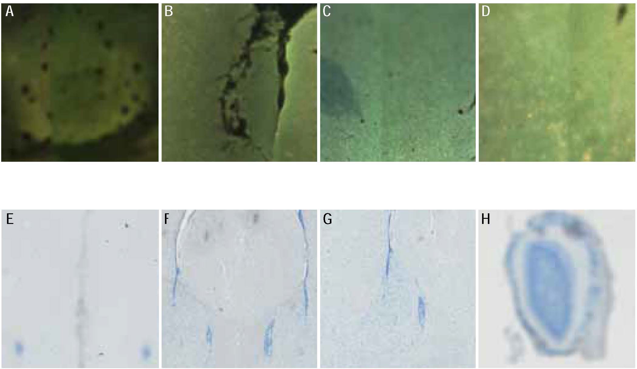
Sample image tiles and their classification with different methods (shown in Table 6).

Table 6:

Classification of sample images using different methods. The steerable filters, Tenengrad, Gaussian derivative, Modified Laplacian and Yang et al. (2018) are denoted as STF, TG, GDR, MLA and NN respectively. Small tiles of the images are shown in Figure 8.

	Panel
Method	a	b	c	d	e	f	g	h
Visual Inspection	OOF	OOF	OOF	OOF	OOF	OOF	OOF	OOF
STF	OOF	OOF	OOF	OOF	OOF	OOF	OOF	OOF
TG	In-focus	In-focus	In-focus	In-focus	In-focus	In-focus	In-focus	OOF
GDR	In-focus	In-focus	In-focus	In-focus	In-focus	In-focus	In-focus	OOF
MLA	OOF	In-focus	OOF	In-focus	OOF	OOF	OOF	OOF
NN	OOF	OOF	OOF	In-focus	In-focus	OOF	OOF	OOF

The image quality score BRISQUE (Mittal et al., 2012) was also tested for automatic detection of OOF images in our datasets. This image evaluator does not require a reference image to evaluate image quality so the only information that the algorithm receives is the spatial information from the image whose quality is being assessed. A smaller BRISQUE score indicates better image quality. Figure 9 shows a comparison of three different methods (SML, BRISQUE, STF) for a particular fluorescent dataset. The data points in the red asterisk denote the OOF images that were identified through visual inspection. Compared with the other two methods, the STF metric is clearly superior in differentiating the OOF and in-focus images while the SML metric places some OOF images close to the main branch which could cause those images to be characterized as in-focus by the outlier detection algorithm. We expect the OOF images to have higher BRISQUE scores than images that are not OOF but in Figure 9b the images that are confirmed as OOF through visual inspection are not grouped together and are scattered in different locations of the plot. Therefore, the BRISQUE metric would not be appropriate to be used for the purpose of locating OOF images in our datasets as the plot of the metric can not be used to differentiate between the two classes of images.

Figure 9:

Different methods for identifying OOF images in a fluorescent dataset. The red asterisks (*) denote the images that were identified as OOF visually. The STF metric clearly differentiates the OOF and in-focus images while the SML metric places four images close to the main branch so the outlier detection will classify them as in-focus. The middle panel shows the BRISQUE scores for all images in the dataset. We notice that there is no pattern for our visual OOF images, some of them are closer to one and some are close to the smaller values of the dataset. A smaller BRISQUE score indicates a better quality image so we expect the OOF images to be clustered towards the highest values. Therefore this metric would not be appropriate for our dataset since there is no consistency in the location of the OOF images.

4. Wider applications

We have demonstrated that the STF method can be used to successfully recognize OOF images from brain image datasets. This method can also be used to identify OOF images from a sequence of images, for example series of rapid succession (burst) images from a still camera, image stills extracted from videos or histology image stacks. To demonstrate the general applicability of the method, we used a publicly available dataset of tissue sections of a mouse prostate (Kartasalo et al., 2018). The whole slide image datasets are located in http://urn.fi/urn:nbn:fi:csc-kata20170705131652639702. The stack contains 260 serial tissue sections scanned at 20X. We randomly chose ten images from the stack and used different filters to artificially create OOF images (Campanella et al., 2018; Bray et al., 2012). We used a 2D Gaussian smoothing kernel of varying widths (standard deviations of 7, 3, 5) for images 15, 22, 152 and a 2D smoothing kernel of the same width (standard deviation 5) at 25% and 50% of images 79 and 99 respectively. Additionally, we blurred images 62, 142, 143 and images 180, 219 with varying sizes of median filters and average filters respectively. The images are depicted in Figure 10, for comparison we have included two in-focus images (sections 21 and 181). The outlier detection plot is shown in Figure 11.

Figure 10:

Color images of tissue sections of a mouse prostate (Kartasalo et al., 2018). All images, except sections 21 and 181 that are used for comparison, were artificially blurred with different kernels.

Figure 11:

Outlier detection plot with our proposed method. The black (◊) symbol represents all the data, the blue line is the moving median and the red (◊) data points are the simulated OOF images which were identified as OOF from our algorithm.

Knowing which images are OOF allowed us to confirm whether the method was successful or not. We calculated the FV for all the images and we located the outliers using a moving median as we discussed in Sec. 2.2.3 (similar to applying a Hampel filter (Pearson, 2002)). The OOF images we created coincided with the images that were identified as outliers, proving the efficacy of our method. We also attempted to locate the outliers using an alternative method such as the quantile regression (Koenker et al., 2005), since the FV data series cannot be modeled after a particular curve as it can vary in different data sets. The quantile regression estimates the conditional median or other quantiles around the response variable, which is more robust to outliers. The advantage of this method is that the result is a distribution that can used to infer the outliers and therefore the OOF candidates. The results however were mixed, and when tested with our brain datasets the algorithm failed to identify several of the outliers, especially partially OOF images, so this method was not deemed appropriate to be used in our pipeline.

5. Discussion

Quality control is a necessary part of an image processing workflow and removing OOF images that can influence the quality and accuracy of subsequent cell segmentation algorithms is an essential part of the preprocessing pipeline. Due to the large volume of data produced in our project, any method to remove OOF images ideally should not require user intervention and can be automated to speed the workflow. The method we presented requires initially to extract the sample from the background, calculate a metric and finally locate any outliers from each stack. Despite the fact that the edge detection and the STF metric require a few parameters to be defined (such as the size of the median filter for the edge detection and the kernel size for the STF metric), once they are estimated the algorithm can be automated to run in a pipeline without any user intervention. Our method utilizes each whole brain image dataset in order to impose a dynamic threshold, as opposed to imposing a specific numeric threshold to make that classification, because using an empirical value was not found to be advantageous. The use of an empirical value as a threshold would allow us to classify the images in real time without using the whole stack but it has many drawbacks and can lead to erroneous characterizations. Estimating an empirical threshold would require inspection of a large number of images which would be very time consuming and could introduce a large uncertainty. Additionally, a specific threshold might not be accurate for all the brain image datasets due to changes in illumination and modalities. However, these are not considered varied within each stack so the assumption is that neighboring sections should have relatively consistent focus values as they have sufficient spatial correlation. Therefore, local outliers are considered OOF images and since this method identifies outliers the assumption is that the OOF images are the minority in each brain image dataset. If a brain image dataset includes a majority of OOF images, the results will not be reliable but such an image dataset will otherwise have to be discarded because the data would be unusable.

In order to demonstrate that our method can be used in a variety of datasets we have used a publicly available dataset (Kartasalo et al., 2018) and used a selection of the image sections to simulate OOF images. The timing of the proposed method is considerably faster than visual inspection and can be accelerated by running computations in parallel. For instance, an image of a tissue size 12000 × 10000 pixels required 12 seconds to run the analysis with our computational resources (Intel Xeon E5–2665 running at 2.40GHz) and by utilizing MATLAB (MATLAB, 2018). Therefore, it takes roughly an hour to complete the analysis for a brain image dataset of 300 images with our computational resources. In a stack of 300 images (where only a very small number of images are OOF) the amount of time it will take for even an experienced observer to inspect all images in smaller tiles will be considerably larger. For instance, a typical image may take up to 1–2 minutes of visual inspection to reach a conclusion and all the images in each given stack would have to be inspected in such a manner. Clearly, the automated method significantly accelerates the OOF detection.

6. Conclusion

We have presented a method to identify OOF images from serial tissue sections. The images presented were generated using a NanoZoomer 2.0 HT (Hamamatsu/Olympus) automated slide scanning microscope but the method can be used for many different digital scanners. After extensive testing we concluded that the method achieves OOF image classification with recall equal to 1 and precision ranging from 0.91 to 0.97 depending on the modality. For most of the brain image datasets that were analyzed, it accurately identifies only the images that are OOF, while for the remaining datasets the method identifies at most two false positives. The program is currently being used successfully in production and it allows us to label and remove the OOF images before they can be used in any further analyses and to replace the OOF images with new, in-focus images.

Our method allows for image classification that is not dependent on the skill of the observer and is significantly faster than visual inspection. The main disadvantage of the method is that each image stack has to be analyzed together and therefore is not suitable for real time analysis. However, our method can have wider medical applications as well as applications to video frame captures, burst images or any other series of images.

Highlights.

• A new method of identifying out-of-focus images in serial tissue sections is proposed.

• The method combines steerable filters and outliers detection to locate out-of-focus images.

• Comparisons with visual inspections show the method has high recall and precision.

• The method outperforms others and can be used for a variety of datasets.

• The method can be automated and implemented in a pipeline.

Appendix A. Focus metrics

A short description of the additional metrics which we used in the paper follows. I denotes the original image while * denotes the convolution of the image with a mask.

1. Gaussian Derivative

The focus measure is based on the first order Gaussian derivative (Geusebroek et al., 2000)

$$F_{GD}=\sum _{x,y}{\left(I*G_x\right)}^2+{\left(I*G_y\right)}^2,$$ (A.1)

where G_x and G_y are the x and y partial derivatives of the Gaussian function respectively. The Gaussian function is defined as

$$G(x,y)=\frac{1}{2\pi {\sigma }^2}{e}^{-\frac{(x^2+y^2)}{2{\sigma }^2}}$$ (A.2)

2. Tenengrad

The focus metric is derived by initially convolving the image with Sobel operators. The images that result from this operation are denoted as S_x and S_y for each pixel in position (x, y). The metric is derived by summing the square of the components of the vector (Krotkov & Martin, 1986)

$$F_{TN}=\sum _{height}\sum _{width}{S}_x{(x,y)}^2+S_y{(x,y)}^2$$ (A.3)

3. Modified Laplacian

If we apply convolution to the image using the modified Laplacian convolution masks L_x = [−1 2 − 1] and $L_y=L_x^T$, the focus metric is the sum of the absolute values of that convolution (Nayar & Nakagawa, 1994)

$$F_{SML}=\sum _{height}\sum _{width}\left|I*L_x\right|+\left|I*L_y\right|$$ (A.4)

Appendix B. Matlab Code for Focus Value

Appendix C. Flowchart

Figure C.12:

Flowchart of our proposed method.

References

- Barker J, Hoogi A, Depeursinge A, & Rubin DL (2016). Automated classification of brain tumor type in whole-slide digital pathology images using local representative tiles. Medical image analysis, 30, 60–71. [DOI] [PubMed] [Google Scholar]
- Bohland JW, Wu C, Barbas H, Bokil H, Bota M, Breiter HC, Cline HT, Doyle JC, Freed PJ, Greenspan RJ et al. (2009). A proposal for a coordinated effort for the determination of brainwide neuroanatomical connectivity in model organisms at a mesoscopic scale. PLoS computational biology, 5, e1000334. [DOI] [PMC free article] [PubMed] [Google Scholar]
- Bray M-A, & Carpenter A (2017). Imaging Platform, Broad Institute of MIT and Harvard. Advanced Assay Development Guidelines for Image-Based High Content Screening and Analysis. 2017 Jul 8., In: Sittampalam GS, Grossman A, Brimacombe K, et al. , editors. Assay Guidance Manual [Internet]. Bethesda (MD): Eli Lilly and Company and the National Center for Advancing Translational Sciences; 2004-. Available from: https://www.ncbi.nlm.nih.gov/books/NBK126174/. [PubMed]
- Bray M-A, Fraser AN, Hasaka TP, & Carpenter AE (2012). Workflow and metrics for image quality control in large-scale high-content screens. Journal of biomolecular screening, 17, 266–274. [DOI] [PMC free article] [PubMed] [Google Scholar]
- Campanella G, Rajanna AR, Corsale L, Schüffler PJ, Yagi Y, & Fuchs TJ (2018). Towards machine learned quality control: A benchmark for sharpness quantification in digital pathology. Computerized Medical Imaging and Graphics, 65, 142–151. [DOI] [PMC free article] [PubMed] [Google Scholar]
- Canny J (1986). A computational approach to edge detection. IEEE Transactions on pattern analysis and machine intelligence, 8, 679–698. [PubMed] [Google Scholar]
- Farahani N, Parwani AV, & Pantanowitz L (2015). Whole slide imaging in pathology: advantages, limitations, and emerging perspectives. Pathol Lab Med Int, 7, 23–33. [Google Scholar]
- Freeman WT, & Adelson EH (1991). The design and use of steerable filters. IEEE Transactions on Pattern Analysis & Machine Intelligence, 13, 891–906. [Google Scholar]
- Geusebroek J-M, Cornelissen F, Smeulders AW, & Geerts H (2000). Robust autofocusing in microscopy. Cytometry: The Journal of the International Society for Analytical Cytology, 39, 1–9. [PubMed] [Google Scholar]
- Gonzalez RC, & Woods RE (2006). Digital Image Processing (3rd Edition). Upper Saddle River, NJ, USA: Prentice-Hall, Inc. [Google Scholar]
- Huang W, & Jing Z (2007). Evaluation of focus measures in multi-focus image fusion. Pattern recognition letters, 28, 493–500. [Google Scholar]
- Kartasalo K, Latonen L, Vihinen J, Visakorpi T, Nykter M, & Ruusuvuori P (2018). Comparative analysis of tissue reconstruction algorithms for 3d histology. Bioinformatics, 34, 3013–3021. [DOI] [PMC free article] [PubMed] [Google Scholar]
- Koenker R, Chesher A, & Jackson M (2005). Quantile Regression. Econometric Society Monographs. Cambridge University Press. [Google Scholar]
- Krotkov E, & Martin J-P (1986). Range from focus. Proceedings IEEE International Conference on Robotics and Automation. IEEE-CS:1093–1098. [Google Scholar]
- MATLAB (2018). version 9.4 (R2018a). Natick, Massachusetts: The MathWorks Inc. [Google Scholar]
- Minhas R, Mohammed AA, & Wu QJ (2012). An efficient algorithm for focus measure computation in constant time. IEEE transactions on circuits and systems for video technology, 22, 152–156. [Google Scholar]
- Minhas R, Mohammed AA, Wu QJ, & Sid-Ahmed MA (2009). 3D shape from focus and depth map computation using steerable filters. In Kamel M, Campilho A (eds). Image Analysis and Recognition. ICIAR 2009. Lecture Notes in Computer Science, vol. 5627. Springer, Berlin, Heidelberg. [Google Scholar]
- Mitra PP (2014). The circuit architecture of whole brains at the mesoscopic scale. Neuron, 83, 1273–1283. [DOI] [PMC free article] [PubMed] [Google Scholar]
- Mittal A, Moorthy AK, & Bovik AC (2012). No-reference image quality assessment in the spatial domain. IEEE Transactions on image processing, 21, 4695–4708. [DOI] [PubMed] [Google Scholar]
- Mukhopadhyay S, Feldman MD, Abels E, Ashfaq R, Beltaifa S, Cacciabeve NG, Cathro HP, Cheng L, Cooper K, Dickey GE et al. (2018). Whole slide imaging versus microscopy for primary diagnosis in surgical pathology: a multicenter blinded randomized noninferiority study of 1992 cases (pivotal study). The American journal of surgical pathology, 42, 39. [DOI] [PMC free article] [PubMed] [Google Scholar]
- Nayar S, & Nakagawa Y (1994). Shape from focus. IEEE Transactions on Pattern Analysis and Machine Intelligence, 16, 824–831. [Google Scholar]
- Otsu N (1979). A threshold selection method from gray-level histograms. IEEE transactions on systems, man, and cybernetics, 9, 62–66. [Google Scholar]
- Pearson RK (2002). Outliers in process modeling and identification. IEEE Transactions on control systems technology, 10, 55–63. [Google Scholar]
- Pertuz S, Puig D, & Garcia MA (2013). Analysis of focus measure operators for shape-from-focus. Pattern Recognition, 46, 1415–1432. [Google Scholar]
- Pinskiy V, Jones J, Tolpygo AS, Franciotti N, Weber K, & Mitra PP (2015). High-throughput method of whole-brain sectioning, using the tape-transfer technique. PloS one, 10, e0102363. [DOI] [PMC free article] [PubMed] [Google Scholar]
- Pinskiy V, Tolpygo AS, Jones J, Weber K, Franciotti N, & Mitra PP (2013). A low-cost technique to cryo-protect and freeze rodent brains, precisely aligned to stereotaxic coordinates for whole-brain cryosectioning. Journal of neuroscience methods, 218, 206–213. [DOI] [PMC free article] [PubMed] [Google Scholar]
- Prewitt JM (1970). Object enhancement and extraction. Picture processing and Psychopictorics, 10, 15–19. [Google Scholar]
- Roberts LG (1963). Machine perception of three-dimensional solids. Technical report, 315, MIT Lincoln Laboratory, Ph. D. Dissertation. [Google Scholar]
- Saco A, Diaz A, Hernandez M, Martinez D, Montironi C, Castillo P, Rakislova N, del Pino M, Martinez A, & Ordi J (2017). Validation of whole-slide imaging in the primary diagnosis of liver biopsies in a university hospital. Digestive and Liver Disease, 49, 1240–1246. [DOI] [PubMed] [Google Scholar]
- Senaras C, Niazi MKK, Lozanski G, & Gurcan MN (2018). Deepfocus: Detection of out-of-focus regions in whole slide digital images using deep learning. PloS one, 13, e0205387. [DOI] [PMC free article] [PubMed] [Google Scholar]
- Shah M, Mishra S, Sarkar M, & Rout C (2017). Identification of robust focus measure functions for the automated capturing of focused images from ziehl–neelsen stained sputum smear microscopy slide. Cytometry Part A, 91, 800–809. [DOI] [PubMed] [Google Scholar]
- Xia X, Yao Y, Liang J, Fang S, Yang Z, & Cui D (2016). Evaluation of focus measures for the autofocus of line scan cameras. Optik, 127, 7762–7775. [Google Scholar]
- Yang SJ, Berndl M, Ando DM, Barch M, Narayanaswamy A, Christiansen E, Hoyer S, Roat C, Hung J, Rueden CT et al. (2018). Assessing microscope image focus quality with deep learning. BMC bioinformatics, 19, 77. [DOI] [PMC free article] [PubMed] [Google Scholar]